A zero-inflated endemic-epidemic model with an application to measles time series in Germany

Abstract

Count data with excessive zeros are often encountered when modelling infectious disease occurrence. The degree of zero inflation can vary over time due to non-epidemic periods as well as by age group or region. The existing endemic-epidemic modelling framework (aka HHH) lacks a proper treatment for surveillance data with excessive zeros as it is limited to Poisson and negative binomial distributions. In this paper, we propose a multivariate zero-inflated endemic-epidemic model with random effects to extend HHH. Parameters of the new zero-inflation and the HHH part of the model can be estimated jointly and efficiently via (penalized) maximum likelihood inference using analytical derivatives. A simulation study confirms proper convergence and coverage probabilities of confidence intervals. Applying the model to measles counts in the 16 German states, 2005–2018, shows that the added zero-inflation improves probabilistic forecasts.

Keywords: zero inflation, multivariate time series, epidemic modelling, seasonality, measles

1 Introduction

Infectious disease models help to understand the mechanisms of disease spread and can be used to generate forecasts. The endemic-epidemic modelling approach of Held et al., (2005), aka the HHH model (after the authors’ initials), is frequently adopted for time series of infectious disease counts. It is motivated by a branching process with immigration in that it decomposes disease incidence into endemic and autoregressive parts. The comprehensive R package surveillance (Meyer et al.,, 2017) provides tools for model estimation, simulation and visualization. The HHH model has been applied to a variety of infectious diseases, including norovirus gastroenteritis (Meyer and Held,, 2017), invasive pneumococcal disease (Chiavenna et al.,, 2019), pertussis (Munro et al.,, 2020), and COVID-19 (Dickson et al.,, 2020; Giuliani et al.,, 2020; Ssentongo et al.,, 2021).

Count data with excessive zeros are often encountered in public health surveillance of rare diseases, such as syphilis in the USA (Yang et al.,, 2013), visceral leishmaniasis at block level in India (Nightingale et al.,, 2020), or dengue fever in China (Wang et al.,, 2014) or Brazil (Schmidt and Pereira,, 2011). Zero-inflated and hurdle models are typically used to analyze such data. Rose et al., (2006) conclude that the choice between a zero-inflated and a hurdle model should generally be driven by the study purpose and the assumed underlying process. A zero-inflated model, as a mixture model, assumes two underlying disease processes: zeros are generated both from the at-risk population (sampling zeros) and the not-at-risk population (structural zeros). A hurdle model, on the other hand, considers all zeros coming from the at-risk population. For counts of infections, zero-inflated models are more appropriate than hurdle models because a large not-at-risk population may exist, e.g., those immunized by vaccination or recovery, or a community which is detached from an outbreak area.

To account for the not-at-risk population, we propose an extension of the HHH approach for infectious disease time series with excessive zeros: a multivariate zero-inflated HHH model. The zero-inflation part can capture seasonality but also autoregressive effects to reflect that zeros become more likely with fewer past counts. The HHH part of the mixture uses the same endemic-epidemic decomposition as in the original HHH model. Region-specific random effects are allowed in both parts to account for heterogenous reporting or varying infection risks, for example due to demographic factors not covered by covariates.

This paper is organized as follows. Section 2 describes the proposed modelling and inference approach, which is evaluated with a simulation study in Section 3. In Section 4 we investigate different zero-inflated models for measles data from Germany and compare their forecast performance with classical HHH models. Section 5 concludes the paper.

2 Model formulation and inference

2.1 Endemic-epidemic modelling

The so-called HHH model (Held et al.,, 2005; Paul and Held,, 2011) assumes that the number of new cases $Y_{rt}$ of a (notifiable) infectious disease in unit $r$, $r=1,\dots,R$ at time $t$, $t=1,\dots,T$, given the past counts, follows a negative binomial distribution,

$$Y_{rt}|\mathcal{F}_{t-1}\sim\operatorname{NB}(\mu_{rt},\psi_{r}),$$

with conditional mean $\mu_{rt}$ and conditional variance $\mu_{rt}(1+\psi_{r}\mu_{rt})$. Here, $\mathcal{F}_{t-1}=\sigma(Y_{1},\dots,Y_{t-1})$ represents the information up to time $t-1$, and $\psi_{r}>0$ are unit-specific overdispersion parameters, possibly assuming $\psi_{r}\equiv\psi$. Units typically correspond to geographical regions, age groups, or the interaction of both (Meyer and Held,, 2017).

The endemic-epidemic modelling approach then decomposes the infection risk additively into an autoregressive component (for within-unit transmission), a spatiotemporal or neighbourhood component (for transmission from other units), and an endemic component (for cases not directly linked to previously observed cases). The endemic component is sometimes called background risk, environmental reservoir, or immigration component. More specifically, the expected number of new cases $\mu_{rt}$ is modelled as

$$\mu_{rt}=\lambda_{rt}y_{r,t-1}+\phi_{rt}\sum_{q\neq r}w_{qr}y_{q,t-1}+\nu_{rt},$$ (1)

where $\lambda_{rt}>0$ is the autoregressive parameter, $\phi_{rt}>0$ is the spatiotemporal parameter linking region $r$ to neighbouring regions via transmission weights $w_{qr}$ (possibly unknown as in Meyer and Held,, 2014), and $\nu_{rt}>0$ is the endemic component. All three parameters are modelled on the log scale as

$$\log(\lambda_{rt}) =\alpha^{(\lambda)}+b_{r}^{(\lambda)}+\bm{x}_{rt}^{(\lambda)T}\bm{\beta}^{(\lambda)}+\log\big{(}o_{rt}^{(\lambda)}\big{)},$$

$$\log(\phi_{rt}) =\alpha^{(\phi)}+b_{r}^{(\phi)}+\bm{x}_{rt}^{(\phi)T}\bm{\beta}^{(\phi)}+\log\big{(}o_{rt}^{(\phi)}\big{)},$$

$$\log(\nu_{rt}) =\alpha^{(\nu)}+b_{r}^{(\nu)}+\bm{x}_{rt}^{(\nu)T}\bm{\beta}^{(\nu)}+\log\big{(}o_{rt}^{(\nu)}\big{)},$$

where in each component, $\alpha^{(\cdot)}$ and $b_{r}^{(\cdot)}$ are fixed and zero-mean random intercepts, respectively, $\bm{\beta}^{(\cdot)}$ is a vector of unknown coefficients for the covariates $\bm{x}_{rt}^{(\cdot)}$, and $o_{rt}^{(\cdot)}$ is an optional offset, e.g., population fractions $o_{rt}^{(\nu)}=n_{rt}/n_{.t}$ in the endemic component.

Likelihood inference for HHH models and many of its extensions is implemented in the R package surveillance (Meyer et al.,, 2017), which also contains several example datasets and corresponding vignettes for illustration.

2.2 Zero-inflated HHH model

To account for excess zeros in surveillance time series, we propose to extend the above HHH model to a zero-inflated model, which we will call HHH4ZI. For this purpose, we assume the number of new cases $Y_{rt}$ given $\mathcal{F}_{t-1}$ to follow a zero-inflated (ZI) negative binomial distribution (Yau et al.,, 2003). Its probability mass function is given by

$$f_{ZI}(y_{rt};\mu_{rt},\psi_{r},\gamma_{rt})=\gamma_{rt}\cdot\mathbf{1}_{\{0\}}(y_{rt})+(1-\gamma_{rt})\cdot f(y_{rt};\mu_{rt},\psi_{r}),$$ (2)

which represents a mixture of a point mass at zero and a HHH model with probability mass function $f(y_{rt};\mu_{rt},\psi_{r})$, i.e., a $\operatorname{NB}(\mu_{rt},\psi_{r})$ distribution. The zero-inflation parameter $\gamma_{rt}$ describes the probability that a zero count comes from the degenerate distribution. If $\gamma_{rt}\equiv 0$, the mixture model would reduce to a HHH model. Otherwise, a proportion $\gamma_{rt}\in(0,1)$ of the population is assumed to be not at risk of infection, while infections in the remaining population follow a HHH model.

Simple zero-inflated models assume $\gamma_{rt}\equiv\gamma$ with a single parameter. However, we will typically model the logit-proportion with a linear predictor,

$$\operatorname{logit}(\gamma_{rt})=\alpha^{(\gamma)}+b_{r}^{(\gamma)}+\bm{x}_{rt}^{(\gamma)T}\bm{\beta}^{(\gamma)},$$ (3)

including an intercept $\alpha^{(\gamma)}$, random unit-specific deviations $b_{r}^{(\gamma)}$, and covariate effects, similar to the parameters $\lambda_{rt}$, $\phi_{rt}$, and $\nu_{rt}$ of the HHH mean $\mu_{rt}$. For example, yearly seasonality can be modelled via $\bm{x}_{rt}^{(\gamma)}=(\sin(\omega t),\cos(\omega t),\dots,\sin(S\cdot\omega t),\cos(S\cdot\omega t))^{\top}$, where $S$ denotes the number of harmonics and $\omega=2\pi/52$ for weekly data, or $\omega=2\pi/26$ for bi-weekly data. Note that, for any $\delta,\zeta\in\mathbb{R}$,

$$\delta\sin(\omega t)+\zeta\cos(\omega t)=A\sin(\omega t+\varphi),$$ (4)

where $A=\sqrt{\delta^{2}+\zeta^{2}}$ is the amplitude and $\varphi=\arctan(\zeta/\delta)$ is the phase shift of a sinusoidal wave. Furthermore, we can relate the zero-inflation probability to past counts to model that (temporary) low incidence tends to inflate the chance of zero cases. Suppose $\bm{x}_{rt}^{(\gamma)}=y_{r,t-1}$, then Equation (3) can be rewritten in terms of the odds $\gamma_{rt}/(1-\gamma_{rt})=\exp(\alpha^{(\gamma)}+b_{r}^{(\gamma)})\exp(\beta^{(\gamma)}y_{r,t-1})$ that the count inherits from the degenerate distribution. One additional case in $y_{r,t-1}$ would change the odds for excess zeros by a factor of $e^{\beta^{(\gamma)}}$, where we would expect $\beta^{(\gamma)}<0$. Note that the odds for excess zeros are intrinsically driven by two opposite forces: Firstly, with higher incidence in a region the probability of contact with an outbreak member increases, such that a larger part of the population is at risk. Secondly, the population immunized by recovery will increase in the long run.

The conditional mean and variance of the zero-inflated model can be easily derived from a hierarchical formulation using a latent Bernoulli variable. Keeping notation simple by omitting the explicit conditioning on $\mathcal{F}_{t-1}$ and random effects, we can write

$$W_{rt} \sim\operatorname{Bernoulli}(\gamma_{rt}),$$

$$Y_{rt}|W_{rt} \sim\operatorname{NB}((1-W_{rt})\,\mu_{rt},\psi_{r}).$$

By the laws of total expectation and variance,

$$\operatorname{E}(Y_{rt})=\operatorname{E}_{W}(E(Y_{rt}|W_{rt}))=\operatorname{E}_{W}((1-W_{rt})\,\mu_{rt})=(1-\gamma_{rt})\,\mu_{rt}$$ (5)

and

$$\operatorname{var}(Y_{rt}) =\operatorname{E}_{W}(\operatorname{var}(Y_{rt}|W_{rt}))+\operatorname{var}_{W}(\operatorname{E}(Y_{rt}|W_{rt}))$$

$$=(1-\gamma_{rt})\,(1+\mu_{rt}\psi_{r}+\gamma_{rt}\mu_{rt})\,\mu_{rt}.$$ (6)

The HHH model allows for the estimation of an effective reproduction number (Bauer and Wakefield,, 2018). For this purpose, the expected non-environmental risk can be written in matrix form as $\bm{A}_{t}\bm{y}_{t-1}$, where $\bm{y}_{t}=(y_{1t},\dots,y_{Rt})^{T}$ and $\bm{A}_{t}$ is a $R\times R$ matrix with diagonal elements $(\bm{A}_{t})_{r,r}=(1-\gamma_{rt})\lambda_{rt}$ and $(\bm{A}_{t})_{r,r^{\prime}}=(1-\gamma_{rt})\phi_{rt}w_{r^{\prime}r}$ for $r\neq r^{\prime}$. The model-based effective reproduction number $R_{t}$ is the dominant eigenvalue of $\bm{A}_{t}$ (Diekmann et al.,, 2012, Part II).

We follow Paul and Held, (2011) by considering two variants for the distribution of the random effects: uncorrelated random effects or within-unit correlation between components. We denote the vector of all random effects from the four components by $\bm{b}=(\bm{b}^{(\lambda)T},\bm{b}^{(\phi)T},\bm{b}^{(\nu)T},\bm{b}^{(\gamma)T})^{T}$, which is assumed to be multivariate normal with mean $\bm{0}$ and covariance matrix $\bm{\Sigma}$. The uncorrelated variant is given by

$$\bm{\Sigma}=\text{blockdiag}(\sigma_{\lambda}^{2}\mathbf{I}_{R},\sigma_{\phi}^{2}\mathbf{I}_{R},\sigma_{\nu}^{2}\mathbf{I}_{R},\sigma_{\gamma}^{2}\mathbf{I}_{R}),$$ (7)

where $\sigma_{\lambda}^{2},\sigma_{\phi}^{2},\sigma_{\nu}^{2},\sigma_{\gamma}^{2}$ are unknown variance parameters for each component and $\mathbf{I}_{R}$ denotes the identity matrix of size $R$. For correlation between different components, the covariance matrix is alternatively defined as

$$\bm{\Sigma}=\bm{\Omega}\otimes\mathbf{I}_{R},$$ (8)

where $\bm{\Omega}\in\mathbb{R}^{4\times 4}$ is an unknown covariance matrix and $\otimes$ denotes the Kronecker product. The positive definiteness of $\bm{\Sigma}$ is ensured if $\bm{\Omega}$ is positive definite (Horn and Johnson,, 1991). The random effects are still uncorrelated between different units. In order to ensure computational efficiency and enforce the positive definiteness of $\bm{\Omega}$, we use a spherical parametrization (Pinheiro and Bates,, 1996; Rapisarda et al.,, 2007). Details can be found in the Appendix.

2.3 Inference

The log-likelihood of a HHH4ZI model without random effects is given by

$$l(\bm{\theta},\bm{\tilde{\psi}})=\sum_{r,t}\log f_{ZI}(y_{rt};\mu_{rt},\psi_{r},\gamma_{rt}),$$ (9)

where $\bm{\theta}=(\alpha^{(\lambda)},\alpha^{(\phi)},\alpha^{(\nu)},\alpha^{(\gamma)},\bm{\beta}^{(\lambda)T},\bm{\beta}^{(\phi)T},\bm{\beta}^{(\nu)T},\bm{\beta}^{(\gamma)T})^{T}$ is the vector of parameters affecting the mean $(1-\gamma_{rt})\mu_{rt}$, and $\bm{\tilde{\psi}}$ is the vector of transformed (unit-specific) overdispersion parameters, using $\tilde{\psi}_{r}=-\log(\psi_{r})$ to allow for unconstrained optimization. The parameters can be estimated by numerical maximization of the log-likelihood $l(\bm{\theta},\bm{\tilde{\psi}})$. We use the quasi-Newton algorithm available as nlminb() in R (R Core Team,, 2020), in conjunction with the analytical gradient and Hessian.

When fitting a HHH4ZI model with random effects, we follow a penalized likelihood approach (Kneib and Fahmeir,, 2007) along the lines of the original HHH model (Paul and Held,, 2011). The penalized log-likelihood is given by

$$l_{\text{pen}}(\bm{\theta},\bm{b},\bm{\tilde{\psi}};\bm{\Sigma})=l(\bm{\theta},\bm{b},\bm{\tilde{\psi}})+\log p(\bm{b}|\bm{\Sigma}),$$ (10)

with

$$l(\bm{\theta},\bm{b},\bm{\tilde{\psi}})=\sum_{r,t}\log f_{ZI}(y_{rt};\mu_{rt},\psi_{r},\gamma_{rt}).$$

As the vector of random effects $\bm{b}$ is assumed to follow a multivariate normal distribution,

$$\log p(\bm{b}|\bm{\Sigma})=-\frac{1}{2}\bm{b}^{T}\bm{\Sigma}(\bm{\theta})^{-1}\bm{b}+\text{const},$$

where we omit additive terms not depending on $\bm{b}$ when optimizing (10). The penalized score function $\mathbf{s}_{\text{pen}}$ and Fisher information matrix $\mathbf{F}_{\text{pen}}$ used for numerical optimization are given in the Appendix.

The full marginal likelihood of the variance parameters is given by

$$L_{\text{marg}}(\bm{\Sigma}) =\int\exp\{l_{\text{pen}}(\bm{\theta},\bm{b},\bm{\tilde{\psi}};\bm{\Sigma})\}d\bm{\theta}d\bm{\tilde{\psi}}d\bm{b}.$$

We apply a Laplace approximation and obtain the marginal log-likelihood

$$l_{\text{marg}}(\bm{\Sigma})\approx l(\bm{\hat{\theta}},\bm{\hat{b}},\bm{\hat{\tilde{\psi}}})-\frac{1}{2}\log|\bm{\Sigma}|-\frac{1}{2}\bm{\hat{b}}^{T}\bm{\Sigma}^{-1}\bm{\hat{b}}-\frac{1}{2}\log|\mathbf{F}_{\text{pen}}(\bm{\hat{\theta}},\bm{\hat{b}},\bm{\hat{\tilde{\psi}_{i}}};\bm{\Sigma})|,$$

where $\bm{\hat{\theta}}$, $\bm{\hat{b}}$ and $\bm{\hat{\tilde{\psi}}}$ are estimates based on a given $\bm{\Sigma}$. As these estimates and thus $l(\bm{\hat{\theta}},\bm{\hat{b}},\bm{\hat{\tilde{\psi}}})$ change only slowly as a function of $\bm{\Sigma}$ (Breslow and Clayton,, 1993; Kneib and Fahmeir,, 2007), the marginal log-likelihood can be approximated as

$$l_{\text{marg}}(\bm{\Sigma})\approx-\frac{1}{2}\log|\bm{\Sigma}|-\frac{1}{2}\bm{b}^{T}\bm{\Sigma}^{-1}\bm{b}-\frac{1}{2}\log|\mathbf{F}_{\text{pen}}(\bm{\theta},\bm{b},\bm{\tilde{\psi}};\bm{\Sigma})|,$$ (11)

where $\bm{b}$, $\bm{\theta}$ and $\bm{\tilde{\psi}}$ are current estimates and do not directly depend on $\bm{\Sigma}$. We use numerically robust Nelder-Mead optimization as implemented in R’s optim() to maximize (11).

Overall, a zero-inflated HHH model with random effects can be estimated via the following algorithm:

1. Initialize the covariance matrix $\bm{\Sigma}$ of the random effects.

2. Given $\bm{\Sigma}$, update $\bm{\theta}$, $\bm{b}$, $\bm{\tilde{\psi}}$ by maximizing the penalized log-likelihood (Equation 10).

3. Given current $(\bm{\theta},\bm{b},\bm{\tilde{\psi}})$, update the covariance matrix $\bm{\Sigma}$ by maximizing the marginal log-likelihood (Equation 11) with respect to its spherical parameters (see Appendix).

4. Iterate steps 2 and 3 until convergence.

An R package implementing this method is provided in the supplementary material.

3 Simulation

We conducted a simulation study with $N=1000$ repetitions for different time series lengths $T\in\{50,100,500\}$. The data-generating process was a multivariate HHH4ZI model for the 16 German states using $\alpha^{(\lambda)}=-0.3$, $\alpha^{(\phi)}=0.5$, $\alpha^{(\nu)}=0.5$ $\alpha^{(\gamma)}=0.2$, zero-inflation terms $\bm{x}_{rt}^{(\gamma)}=(\sin(2\pi t/26),\cos(2\pi t/26),y_{r,t-1})^{T}$ with coefficients $\bm{\beta}^{(\gamma)}=(0.4,-0.3,-0.1)^{T}$, homogeneous overdispersion $\psi_{r}=0.5$, and no random effects. We assumed normalized first-order transmission weights, i.e., $w_{qr}=1/m_{q}$, if state $q$ (with $m_{q}$ neighbours) is adjacent to state $r$, and $w_{qr}=0$ otherwise. Furthermore, we used a state-specific offset $o_{r}^{(\phi)}=n_{r}/n_{.}$ such that the rate of imported infections scales with the population size $n_{r}$.

Maximum likelihood estimation converged for all simulated datasets. The estimated parameter vectors are summarized by means and standard deviations in Table 1. As expected, increasing the length of the time series improves the estimates by reducing the variance. Note that the spatio-temporal parameter $\alpha^{(\phi)}$ cannot be estimated reliably from short time series ($T=50$ or 100). A possible reason is that the spatiotemporal component has a relatively small impact on the time series in the assumed model. For long time series ($T=500$), all parameters are estimated reliably. The coverage probability of Wald confidence intervals is approximately equal to their nominal level (95% or 50%) for all parameters and time series lengths.

$T$		$\hat{\alpha}^{(\lambda)}$	$\hat{\alpha}^{(\phi)}$	$\hat{\alpha}^{(\nu)}$	$\hat{\alpha}^{(\gamma)}$	$\hat{\beta}^{(\gamma)}_{1}$	$\hat{\beta}^{(\gamma)}_{2}$	$\hat{\beta}^{(\gamma)}_{3}$	$\hat{\psi}$
50	mean	-0.32	-0.13	0.50	0.20	0.40	-0.31	-0.10	0.49
	SD	0.12	2.79	0.10	0.13	0.13	0.14	0.03	0.10
	coverage 95	95.00	95.60	94.70	95.50	95.10	94.70	94.80	93.40
	coverage 50	49.90	55.40	51.80	52.10	50.80	49.10	49.10	49.90
100	mean	-0.32	0.43	0.50	0.20	0.40	-0.30	-0.10	0.50
	SD	0.08	0.39	0.07	0.09	0.09	0.09	0.02	0.07
	coverage 95	95.10	96.60	95.90	95.60	94.90	94.90	94.80	94.70
	coverage 50	49.50	52.90	51.40	47.30	51.80	52.50	50.50	50.70
500	mean	-0.30	0.49	0.50	0.20	0.40	-0.30	-0.10	0.50
	SD	0.04	0.14	0.03	0.04	0.04	0.04	0.01	0.03
	coverage 95	95.90	96.40	94.40	94.30	95.60	94.90	95.30	94.40
	coverage 50	50.50	50.80	51.80	48.10	49.80	49.30	49.20	48.00

Table 1: Means and standard deviations (SD) of parameter estimates from 1000 simulations for various time series lengths ($T$). Coverage probabilities of 95% and 50% confidence intervals are also given.

4 Application

4.1 Data

We apply the proposed HHH4ZI model to count time series of reported measles cases in the 16 federal states of Germany, from 2005 to 2018. Herzog et al., (2011) have used an earlier version of these data to study the association between measles incidence and vaccination coverage. We follow their approach of aggregating the counts over bi-weekly intervals to approximately match the generation time of measles of around 10 days (Fine and Clarkson,, 1982). Figure 1 shows that measles counts generally remained at low levels with many zeros during off-seasons. However, outbreaks with over 50 cases occurred in several states. The time series of some states, such as Berlin and Brandenburg, suggest a weak biennial cycle. A possible explanation is that susceptibles in low-immune (e.g., anthroposophic) communities (Ernst,, 2011) are depleted during epidemic years. Only minor epidemics may occur throughout the following year when the susceptible population is replenished by births (Dalziel et al.,, 2016).

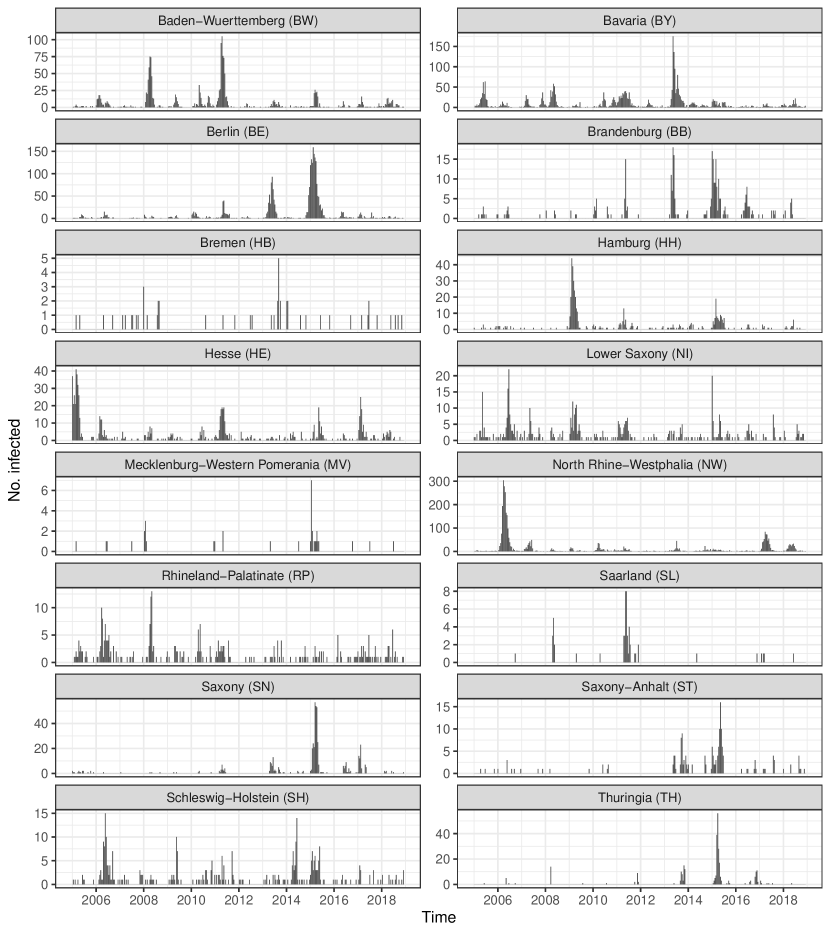
Figure 1: Bi-weekly number of measles cases in the 16 federal states of Germany for the years 2005 to 2018. Note the varying y-axes.

Vaccination coverage is surveyed by local health authorities by checking the receipt of the first and second doses of measles-mumps-rubella (MMR) vaccination among school starters. We assume the coverage rate among children who don’t present a vaccination card at the day of the medical examination (6–14% on average for the different states) to be half of that of children presenting a vaccination card (Herzog et al.,, 2011). These data are currently available until 2018 (before measles vaccination became mandatory in Germany), which is why we restrict our measles analysis to the period from 2005 to 2018.

State	Max	Zeros	Total	Population	Coverage
Baden-Wuerttemberg (BW)	105	147	1 733	10 773 318	89% …90%
Bavaria (BY)	175	66	3 082	12 654 101	88% …93%
Berlin (BE)	159	151	2 533	3 464 046	90% …93%
Brandenburg (BB)	18	276	309	2 498 962	94% …94%
Bremen (HB)	5	324	53	665 379	86% …90%
Hamburg (HH)	44	233	498	1 773 744	90% …94%
Hesse (HE)	41	181	859	6 105 864	91% …95%
Lower Saxony (NI)	22	181	504	7 909 337	91% …93%
Mecklenburg-Western Pomerania (MV)	7	340	36	1 634 664	93% …93%
North Rhine-Westphalia (NW)	304	100	3 641	17 831 720	89% …94%
Rhineland-Palatinate (RP)	13	203	334	4 033 268	90% …94%
Saarland (SL)	8	341	55	1 010 670	91% …93%
Saxony (SN)	57	278	495	4 127 619	95% …93%
Saxony-Anhalt (ST)	16	303	173	2 309 032	93% …93%
Schleswig-Holstein (SH)	15	213	355	2 841 994	89% …92%
Thuringia (TH)	56	321	302	2 212 890	94% …94%

Table 2: Maximum count, number of zeros, total of bi-weekly measles counts, (average) population, and estimated vaccination coverage in 2005 and 2018, for the 16 federal states of Germany.

In Table 2 we compare summary statistics of case counts and vaccination coverage among federal states. The maximum bi-weekly counts range from only 5 (Bremen) to 304 (North Rhine-Westphalia). Periods without any measles cases are rarest in Bavaria (66 bi-weeks), whereas Mecklenburg-Western Pomerania observed no cases at 340 (93.4%) of the 364 time points. Total case numbers correlate strongly with population size, but Berlin experienced relatively large epidemics. The yearly updated state population will serve as an offset in the endemic model component. Relative changes from the beginning to the end of the study period are in the range from -11% (Saxony-Anhalt) to +7% (Berlin). The estimated vaccination coverage varies from 86% (Bremen, 2005) to above 95% (Thuringia, 2008–2012). Germany’s five eastern states (BB, MV, SN, ST, TH) already had a high initial vaccination coverage for historical reasons (measles vaccination was mandatory in the former German Democratic Republic). In the other states, vaccination coverage tended to increase during the investigated period (see Figure S1 in the supplementary material).

4.2 Models

We first consider the simple Poisson HHH model, which Herzog et al., (2011) found to provide the best fit. It included the log proportion of unvaccinated school starters as a covariate in the autoregressive component. This proportion can be regarded as a proxy for the fraction of susceptibles, assuming that one dose of the MMR vaccine already provides full protection. The endemic component contained a sinusoidal wave (4) to capture yearly seasonality, and the standardized state population $n_{rt}$ as an offset. A neighbourhood effect was not included due to the coarse spatial resolution. Indeed, suspected cases and their unprotected contacts are isolated immediately (WHO Regional Office for Europe,, 2013), and the past week’s incidence in adjacent states is much less informative than within-state dynamics. This model, called “P0” in the following, is given by

$$Y_{rt}|\mathcal{F}_{t-1} \sim\operatorname{Po}(\lambda_{rt}y_{r,t-1}+\nu_{rt}),$$

$$\log(\lambda_{rt}) =\alpha^{(\lambda)}+\beta^{(\lambda)}\log(1-x_{rt}),$$

$$\log(\nu_{rt}) =\alpha^{(\nu)}+\delta\sin(2\pi t/26)+\zeta\cos(2\pi t/26)+\log(n_{rt}),$$

where $x_{rt}$ is the estimated vaccination coverage for at least one dose. This means that the local reproduction rate $\lambda_{rt}$ is proportional to (a power of) the fraction of susceptibles, which makes the epidemic component conform to the mass action principle.

Fisher and Wakefield, (2020) proposed an ecological Poisson model, which also incorporates MMR vaccine effectiveness. They used the conditional mean

$$n_{r}(1-\kappa x_{r})(\lambda_{r}y_{r,t-1}/n_{r}+\nu_{rt}),$$

where $\kappa$ is the vaccine effect, $\lambda_{r}$ is the risk of infection and $\nu_{rt}$ is the endemic risk. To take the effect of the varying vaccination coverage into account, we use a similar mean component in the following model extensions. Moreover, we include both yearly and biennial seasonality in both endemic and epidemic components. To account for overdispersion, we also switch to negative binomial distributions with state-specific overdispersion parameters. This model, denoted by “NB1”, is given by

$$Y_{rt}|\mathcal{F}_{t-1} \sim\operatorname{NB}(\lambda_{rt}y_{r,t-1}+\nu_{rt},\psi_{r}),$$

$$\log(\lambda_{rt}) =\alpha^{(\lambda)}+\sum_{s=1}^{2}\left\{\delta_{s}^{(\lambda)}\sin\left(\tfrac{2\pi t}{s\cdot 26}\right)+\zeta_{s}^{(\lambda)}\cos\left(\tfrac{2\pi t}{s\cdot 26}\right)\right\}+\log(1-\kappa x_{rt}),$$

$$\log(\nu_{rt}) =\alpha^{(\nu)}+\sum_{s=1}^{2}\left\{\delta_{s}^{(\nu)}\sin\left(\tfrac{2\pi t}{s\cdot 26}\right)+\zeta_{s}^{(\nu)}\cos\left(\tfrac{2\pi t}{s\cdot 26}\right)\right\}+\log((1-\kappa x_{rt})\,n_{rt}),$$

where $\kappa=0.92$ is the posterior median estimated by Fisher and Wakefield, (2020), and $s=1,2$ corresponds to yearly and biennial seasonality, respectively. To account for unobserved heterogeneity between states, this model is further extended with uncorrelated (“NB2”) or correlated (“NB3”) random effects in both components.

Based on the structure of the models NB1 to NB3, we build several HHH4ZI models of increasing complexity. The simplest extension is “ZI1”, which mixes NB1 with an autoregressive zero-inflation probability $\gamma_{rt}$ via

$$\operatorname{logit}(\gamma_{rt})=\alpha^{(\gamma)}+\beta^{(\gamma)}y_{r,t-1}.$$

Models “ZI2” and “ZI3” are ZI1 models with additional uncorrelated (ZI2) or correlated (ZI3) random effects in endemic, autoregressive and zero-inflation components. By incorporating yearly and biennial seasonality also in the zero-inflation components of models ZI2 and ZI3, we obtain models “ZI4” and “ZI5”, respectively.

4.3 Results

Table 3 summarizes the estimated parameters from the various models. The estimated seasonal amplitudes in the autoregressive part are barely affected by the model updates. The yearly pattern is stronger than the biennial cycle; the combined effect with a peak in calendar weeks 11–12 and a minimum at calendar weeks 39–40 is shown in Figure S2 in the supplementary material. The estimated seasonal effect of the endemic component is very similar, but shrinks when allowing for seasonality of the zero-inflation probability (ZI4 and ZI5). The large overdispersion $\hat{\psi}_{r}$ estimated for some states (Thuringia and Bremen), is considerably reduced by accounting for state-specific zero-inflation probabilities beyond the autoregressive effect (compare ZI1 to ZI2 or ZI3). At the same time, the range of the time-varying effective reproduction number $R_{t}$ increases even more than after introducing state-specific overdispersion. This is due to an improved fit of large outbreaks via the epidemic component in states with otherwise low counts. We observe that $R_{t}$ is estimated to exceed the threshold 1 in January and typically remains below one between June and December (see Figure S3 in the supplementary material). In 2015, $R_{t}$ even peaked at 3.1, which reflects a large measles outbreak among refugees in Berlin (Werber et al.,, 2017). We note that allowing for correlation between random effects increases their variance (NB2 to NB3, ZI2 to ZI3, ZI4 to ZI5). We discuss their spatial variation in the context of model ZI3 further below.

Model	$\hat{\alpha}^{(\lambda)}$	$\hat{\sigma}_{\lambda}$	$\hat{A}_{1}^{(\lambda)}$	$\hat{A}_{2}^{(\lambda)}$	$\hat{\alpha}^{(\nu)}$	$\hat{\sigma}_{\nu}$	$\hat{A}_{1}^{(\nu)}$	$\hat{A}_{2}^{(\nu)}$
P0	0.71 (0.12)				1.92 (0.03)		0.55 (0.04)
NB1	1.38 (0.04)		0.43 (0.05)	0.11 (0.06)	3.98 (0.03)		0.44 (0.05)	0.13 (0.05)
NB2	1.01 – 2.62	0.22	0.44 (0.05)	0.13 (0.06)	3.01 – 7.88	0.48	0.44 (0.05)	0.13 (0.05)
NB3	1.00 – 2.65	0.23	0.44 (0.05)	0.13 (0.06)	3.03 – 7.88	0.48	0.44 (0.05)	0.13 (0.05)
ZI1	1.40 (0.04)		0.42 (0.05)	0.10 (0.06)	4.23 (0.05)		0.41 (0.05)	0.12 (0.05)
ZI2	0.99 – 2.68	0.24	0.44 (0.05)	0.13 (0.06)	3.68 – 9.11	0.63	0.43 (0.05)	0.13 (0.05)
ZI3	0.96 – 2.69	0.27	0.44 (0.05)	0.12 (0.06)	2.96 – 9.10	0.79	0.42 (0.05)	0.14 (0.05)
ZI4	0.99 – 2.71	0.24	0.43 (0.05)	0.12 (0.06)	3.78 – 9.14	0.58	0.37 (0.06)	0.06 (0.06)
ZI5	0.97 – 2.78	0.28	0.43 (0.05)	0.12 (0.06)	3.76 – 9.23	0.66	0.38 (0.06)	0.08 (0.06)

Model	$\hat{\alpha}^{(\gamma)}$	$\hat{\sigma}_{\gamma}$	$\hat{\beta}^{(\gamma)}$	$\hat{A}_{1}^{(\gamma)}$	$\hat{A}_{2}^{(\gamma)}$	$\hat{\psi}_{r}$
P0
NB1						0.49 – 10.27
NB2						0.47 – 10.30
NB3						0.47 – 10.30
ZI1	-1.17 (0.18)		-0.49 (0.09)			0.41 – 8.03
ZI2	-1.95 – 1.45	1.25	-0.73 (0.12)			0.45 – 2.84
ZI3	-3.79 – 1.82	1.77	-0.82 (0.13)			0.31 – 3.38
ZI4	-2.01 – 1.41	1.16	-0.66 (0.11)	0.32 (0.14)	0.26 (0.13)	0.44 – 2.54
ZI5	-1.74 – 1.70	1.37	-0.72 (0.11)	0.26 (0.14)	0.21 (0.14)	0.39 – 3.02

Model	$\hat{\rho}_{\lambda,\nu}$	$\hat{\rho}_{\nu,\gamma}$	$\hat{\rho}_{\lambda,\gamma}$	maxEV	$l_{\text{pen}}$	$l_{\text{marg}}$
P0				0.86 – 1.00	-9299.52
NB1				0.41 – 1.42	-7059.04
NB2				0.40 – 1.52	-6966.87	-92.60
NB3	-0.50			0.40 – 1.52	-6966.51	-91.70
ZI1				0.34 – 1.28	-7037.44
ZI2				0.37 – 2.42	-6914.28	-118.74
ZI3	0.30	0.86	0.62	0.36 – 3.10	-6909.21	-111.99
ZI4				0.36 – 2.23	-6911.89	-125.90
ZI5	0.22	0.70	0.65	0.34 – 2.82	-6908.55	-121.53

Table 3: Parameter estimates (and standard errors) and other summaries of model fit. For region-specific parameters the table shows the range of the point estimates. The time-varying dominant eigenvalue (maxEV) is also summarized by its range. Estimates of $A_{1}^{\cdot}$ and $A_{2}^{\cdot}$ correspond to the amplitudes of the yearly and biennial harmonics, respectively. The $\hat{\rho}_{.,.}$ columns contain the estimated correlations between the different random effect components. For models with random effects, both the penalized log-likelihood $l_{\text{pen}}$ and the marginal log-likelihood ($l_{\text{marg}}$) are given (but note that these should not be used for model selection). For models without random effects, $l_{\text{pen}}$ refers to the standard log-likelihood.

We assessed the quality of one-step-ahead forecasts during the last four years. Several scores are considered (Czado et al.,, 2009): logarithmic score (LS), Dawid-Sebastiani score (DSS), rank probability score (RPS), and squared error score (SES). The logarithmic score is a strictly proper score, whereas the Dawid-Sebastiani score and the rank probability score are proper. The squared error score is a classical measure of forecast performance. It is proper when it is taken as a score for probabilistic forecast (Gneiting et al.,, 2007). However it gives the same score to predictive distributions with the same expectation, regardless of the shape of distributions (Bröcker and Smith,, 2007). The maximum logarithmic score (maxLS) (Ray et al.,, 2017) is not a proper score, but is additionally used to evaluate the worst-case forecast performance. Forecast performance using these scores is compared in Table 4.

Model	LS	p-value	maxLS	DSS	RPS	SES
P0	1.71 (9)	0.00	8.51 (9)	3.24 (9)	1.20 (8)	17.71 (7)
NB1	1.36 (8)	0.00	3.85 (1)	1.88 (6)	1.22 (9)	15.89 (3)
NB2	1.35 (5)	0.01	4.07 (8)	1.94 (8)	1.19 (6)	16.23 (4)
NB3	1.35 (6)	0.01	4.06 (7)	1.94 (7)	1.19 (7)	15.86 (2)
ZI1	1.36 (7)	0.00	3.86 (2)	1.85 (3)	1.18 (5)	15.47 (1)
ZI2	1.34 (3)	0.02	4.05 (6)	1.87 (5)	1.13 (3)	17.66 (6)
ZI3	1.33 (1)		4.04 (5)	1.82 (1)	1.13 (1)	17.21 (5)
ZI4	1.34 (4)	0.03	3.96 (3)	1.86 (4)	1.14 (4)	18.05 (8)
ZI5	1.34 (2)	0.06	3.97 (4)	1.82 (2)	1.13 (2)	18.08 (9)

Table 4: Performance of one-step-ahead forecasts in terms of proper scoring rules: mean log score (LS), maximum log score (maxLS), mean Dawid-Sebastiani score (DSS), mean ranked probability score (RPS) and mean squared error score (SES). Ranks are shown in parantheses. The Monte Carlo p-values for differences in mean log scores are based on 9999 random permutations, comparing each model against the best model.

Models ZI3 and ZI5 consistently produce the best and second-best forecasts in terms of the average LS, DSS and RPS. Based on Monte Carlo permutation tests for differences in mean log scores, model ZI3 significantly outperforms all other models except ZI5. Adding the zero-inflation component consistently improves the aforementioned scores (NB1 to ZI1, NB2 to ZI2 and NB3 to ZI3), where the simple Poisson model ranks last. However, the squared error score ranks models substantially different. Model ZI1 ranks first followed by models NB3, NB1 and NB2. Model ZI5 has the worst mean squared error score. The root mean squared prediction errors of all models are around 4, which means that the forecasts differ from the observed counts by around four cases on average. Looking at the maximum logarithmic score, models have again different ranks. Model NB1 has the best (i.e., lowest) maximum log score, followed by models ZI1, ZI4, ZI5, ZI3 and ZI2. The Poisson model performs much worse at times and on average.

We now focus on model ZI3 and discuss the remaining model parameters. The estimated autoregressive parameter in the zero-inflation component is $\hat{\beta}^{(\gamma)}=-0.82$ (95% CI: [-1.07, -0.57]), which means that each additional case at time $t-1$ decreases the odds of an excess zero at time $t$ by $1-\exp(-0.82)=56\%$. Plots of the fitted time series in Figure S4 (supplementary material) show that model ZI3 fits reasonably well, especially in Brandenburg, Hamburg, Saarland, Saxony-Anhalt and Thuringia. Figure 2 shows maps of the exp-transformed region-specific intercepts estimated from model ZI3. For the endemic and autoregressive components these correspond to rate ratios taking the regional average as a reference, whereas for the zero-inflation component the values correspond to odds ratios. Five states have a relatively high zero-inflation (odds ratio larger than 3): Brandenburg (BB), Saarland (SL), Saxony (SN), Saxony-Anhalt (ST) and Thuringia (TH). Except for Saarland (SL), these states are in East Germany. We notice that these five states have a relatively high vaccination coverage, a low total number of cases (Table 2), but a few outbreaks (Figure 1). This pattern can be accomodated by increasing both the zero-inflation probability and the autoregressive parameter. Correspondingly, these five states also have the largest autoregressive intercepts (rate ratios above 1.18). In contrast, Lower Saxony (NI) and Mecklenburg-Western Pomerania (MV) have the lowest zero inflation. This may relate to a lack of large outbreaks with consistently low counts that would even conform to a negative binomial distribution.

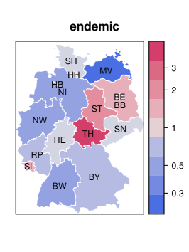
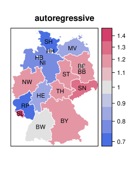
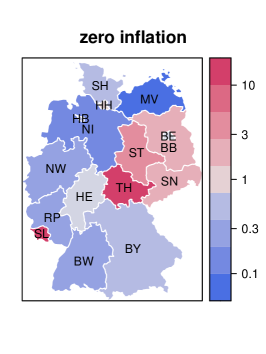
Figure 2: Maps of exp-transformed region-specific intercepts estimated in model ZI3. These correspond to rate ratios (left, center) and odds ratios (right), respectively.

5 Conclusion

We have proposed a multivariate zero-inflated endemic-epidemic model for infectious disease counts with excessive zeros. This model consists of two parts: a zero-inflation part, which represents the not-at-risk population, and a HHH part, which models the at-risk population. The zero-inflation part can incorporate seasonality and autoregressive terms. Its exp-transformed parameters can be interpreted as odds ratios. The HHH part has the same endemic-epidemic decomposition as the classical HHH framework. Random effects are allowed in both parts to account for heterogeneity across units. We applied this model to state-level measles counts in Germany. Both yearly and biennial seasonality are included in our models to capture a potential biennial cycle of measles epidemics. The effect of spatio-temporally varying vaccination coverage is accounted for by assuming the incidence to be proportional to the unvaccinated proportion of school starters. We assessed the forecast performance of this model using proper scoring rules. In comparison with negative binomial models with the same HHH part, zero-inflated HHH models can better capture time series where both low-incidence periods and large outbreaks occur, and the extended models also consistently improve forecast performance.

Conflict of interest

The authors have declared no conflict of interest.

Funding

This work was financially supported by the Interdisciplinary Center for Clinical Research (IZKF) of the Friedrich-Alexander-Universität Erlangen-Nürnberg (FAU), Germany [project J75]. Junyi Lu performed the present work in partial fulfilment of the requirements for obtaining the degree ’Dr. rer. biol. hum.’ at the FAU.

Data availability statement

The data that support the findings of this study were derived from the following resources available in the public domain: case counts from SurvStat@RKI 2.0, Robert Koch Institute (https://survstat.rki.de, accessed 26 March 2021), vaccination coverage from the Information System of the Federal Health Monitoring (https://www.gbe-bund.de/, accessed 23 February 2021), and population data from the Federal Statistical Office of Germany (Statistisches Bundesamt, https://www.destatis.de/, accessed 10 April 2021). The derived datasets are part of the dedicated R package at https://github.com/Junyi-L/hhh4ZI. Code to reproduce all results using that package is provided in the supplementary material.

ORCID

Sebastian Meyer https://orcid.org/0000-0002-1791-9449

Appendix

Parametrization of $\bm{\Sigma}$

When assuming within-unit correlation of the different random effects, we use a spherical parametrization (Pinheiro and Bates,, 1996; Rapisarda et al.,, 2007) for the matrix $\bm{\Omega}$. This enforces positive definiteness and ensures computational efficiency.

We first factorize the covariance matrix $\bm{\Omega}$ by Cholesky decomposition $\bm{\Omega}=\mathbf{D}\mathbf{L}\mathbf{L}^{T}\mathbf{D},$ where $\mathbf{D}=\text{diag}(\sigma_{1},\sigma_{2},\sigma_{3},\sigma_{4})$ is a diagonal matrix with standard deviations (which we estimate on the log scale) and $\mathbf{L}\in\mathbb{R}^{4\times 4}$ is a lower triangular matrix. To ensure the positive definiteness of the covariance matrix, the matrix $\mathbf{L}$ is parametrized by (Rapisarda et al.,, 2007)

$$\mathbf{L}=\begin{pmatrix}1\\ \frac{r_{1}}{\sqrt{r_{1}^{2}+1}}&\frac{1}{\sqrt{r_{1}^{2}+1}}\\ \frac{r_{2}}{\sqrt{r_{2}^{2}+1}}&\frac{r_{3}}{\sqrt{r_{3}^{2}+1}\sqrt{r_{2}^{2}+1}}&\frac{1}{\sqrt{r_{3}^{2}+1}\sqrt{r_{2}^{2}+1}}\\ \frac{r_{4}}{\sqrt{r_{4}^{2}+1}}&\frac{r_{5}}{\sqrt{r_{5}^{2}+1}\sqrt{r_{4}^{2}+1}}&\frac{r_{6}}{\sqrt{r_{6}^{2}+1}\sqrt{r_{5}^{2}+1}\sqrt{r_{4}^{2}+1}}&\frac{1}{\sqrt{r_{6}^{2}+1}\sqrt{r_{5}^{2}+1}\sqrt{r_{4}^{2}+1}}\end{pmatrix},$$

where $r_{1}$, $r_{2}$, $r_{3}$, $r_{4}$, $r_{5}$ and $r_{6}$ are unconstrained parameters.

The log-determinant of $\bm{\Sigma}$, which appears in the marginal log-likelihood $l_{\text{marg}}$, is given by

$$\log|\bm{\Sigma}|=2R\left(\sum_{i=1}^{4}\log\sigma_{i}-\frac{1}{2}\sum_{i=1}^{6}\log(r_{i}^{2}+1)\right).$$

Score function

The score function and Fisher information matrix are derived based on the score function and Fisher information matrix of the HHH model, which can be found in Paul and Held, (2011). We denote the score function of the penalized log-likelihood with respect to the fixed and random parameters by $\mathbf{s}_{\text{pen}}(\bm{\theta},\bm{b},\bm{\tilde{\psi}};\bm{\Sigma})$. It can be partitioned as

$$\bm{s}_{\text{pen}}(\bm{\theta},\bm{b},\bm{\tilde{\psi}};\bm{\Sigma})=\begin{pmatrix}\bm{s}(\bm{\theta})\\ \bm{s}(\bm{\tilde{\psi}})\\ \bm{s}(\bm{b})-\bm{\Sigma}^{-1}\bm{b}\end{pmatrix},$$

where $\bm{s}(\bm{i})=\frac{\partial l(\bm{\theta},\bm{b},\bm{\tilde{\psi}})}{\partial\bm{i}}$ corresponds to the unpenalized score vector with respect to the parameter vector $\bm{i}$. We define $\bm{\xi}^{(\nu)}=(\alpha^{(\nu)},\bm{\beta}^{(\nu)T},\bm{b}^{(\nu)T)})^{T}$ as the vector of parameters of fixed and random effects in the endemic ($\nu$) component. Vectors $\bm{\xi}^{(\lambda)}$, $\bm{\xi}^{(\phi)}$ and $\bm{\xi}^{(\gamma)}$ are defined analogously. We denote by $l_{rt}(\bm{\theta},\bm{b},\tilde{\psi}_{r})=\log f_{ZI}(y_{rt};\mu_{rt},\psi_{r},\gamma_{rt})$ the terms of the unpenalized log-likelihood of the zero-inflated model, and by $l_{rt}^{H}(\mu_{rt},\tilde{\psi}_{r})=\log f(y_{rt};\mu_{rt},\psi_{r})$ the terms of the unpenalized log-likelihood of the original HHH model.

For $\bm{i}=\bm{\xi}^{(\nu)}$, $\bm{\xi}^{(\lambda)}$, $\bm{\xi}^{(\phi)}$, $\bm{\tilde{\psi}}$,

$$\bm{s}(\bm{i})=\sum_{rt}\exp(-l_{rt}(\bm{\theta},\bm{b},\tilde{\psi}_{r}))(1-\gamma_{rt})f(y_{rt},\mu_{rt},\psi_{r})\frac{\partial l^{H}_{rt}(\mu_{rt},\tilde{\psi}_{r})}{\partial\bm{i}},$$

and

$$\bm{s}(\bm{\xi}^{(\gamma)})=\sum_{rt}\exp(-l_{rt}(\bm{\theta},\bm{b},\tilde{\psi}_{r}))(\mathbf{1}_{\{0\}}(y_{rt})-f(y_{rt},\mu_{rt},\psi_{r}))\frac{\partial\gamma_{rt}}{\bm{\xi}^{\gamma}}.$$

We denote $g(x)=\frac{\exp(x)}{\exp(x)+1}$, and $g^{\prime}(x)=\frac{\exp(x)}{(\exp(x)+1)^{2}}$, $g^{\prime\prime}(x)=\frac{\exp(x)(1-\exp(x))}{(\exp(x)+1)^{3}}$. Then $\gamma_{rt}=g(\bm{\xi}^{(\gamma)T}\bm{u}_{rt}^{(\gamma)})$, where $\bm{u}_{rt}^{(\gamma)}=(1,\bm{x}_{rt}^{(\gamma)T},\bm{z}_{rt}^{(\gamma)T})^{T}$, and $\bm{z}_{rt}^{(\gamma)T}$ is a unit vector with $r$-th element being 1. We then have $\frac{\partial\gamma_{rt}}{\partial\bm{\xi}^{(\gamma)}}=g^{\prime}(\bm{\xi}^{(\gamma)T}\bm{u}_{rt}^{(\gamma)})\bm{u}_{rt}^{(\gamma)}$, and $\frac{\partial^{2}\gamma_{rt}}{\partial\bm{\xi}^{(\gamma)}\partial\bm{\xi}^{(\gamma)T}}=g^{\prime\prime}(\bm{\xi}^{(\gamma)T}\bm{u}_{rt}^{(\gamma)})\bm{u}_{rt}^{(\gamma)}\bm{u}_{rt}^{(\gamma)^{T}}.$

Fisher information matrix

The observed Fisher information matrix can be partitioned as

$$\mathbf{F}_{\text{pen}}(\bm{\theta},\bm{b},\bm{\tilde{\psi}};\bm{\Sigma})=\begin{pmatrix}\mathbf{F}_{\text{pen}}[\bm{\theta},\bm{\theta}]&\mathbf{F}_{\text{pen}}[\bm{\theta},\bm{b}]&\mathbf{F}_{\text{pen}}[\bm{\theta},\bm{\tilde{\psi}}]\\ \mathbf{F}_{\text{pen}}[\bm{b},\bm{\theta}]&\mathbf{F}_{\text{pen}}[\bm{b},\bm{b}]+\bm{\Sigma}^{-1}&\mathbf{F}_{\text{pen}}[\bm{b},\bm{\tilde{\psi}}]\\ \mathbf{F}_{\text{pen}}[\bm{\tilde{\psi}},\bm{\theta}]&\mathbf{F}_{\text{pen}}[\bm{\tilde{\psi}},\bm{b}]&\mathbf{F}_{\text{pen}}[\bm{\tilde{\psi}},\bm{\tilde{\psi}}]\end{pmatrix},$$

where $\mathbf{F}_{\text{pen}}[\bm{i},\bm{j}]=-\frac{\partial^{2}l(\bm{\theta},\bm{b},\bm{\tilde{\psi}})}{\partial\bm{i}\partial\bm{j}^{T}}$ denotes the block of the unpenalized Fisher information matrix corresponding to the parameter vectors $\bm{i}$ and $\bm{j}$. For $\bm{i},\bm{j}=\bm{\xi}^{(\lambda)}$, $\bm{\xi}^{(\phi)}$, $\bm{\xi}^{(\nu)}$, or $\bm{\tilde{\psi}}$,

$$\mathbf{F}_{\text{pen}}[\bm{i},\bm{j}] =\mathbf{F}_{\text{pen}}[\bm{j},\bm{i}]=-\sum_{rt}(1-\gamma_{rt})f(y_{rt},\mu_{rt},\psi_{r})\exp(-l_{rt}(\bm{\theta},\bm{b},\tilde{\psi}_{r}))$$

$$\bigg{[}-\exp(-l_{rt}(\bm{\theta},\bm{b},\tilde{\psi}_{r}))(1-\gamma_{rt})f(y_{rt},\mu_{rt},\psi_{r})\frac{\partial l^{H}_{rt}(\mu_{rt},\tilde{\psi}_{r})}{\partial\bm{j}}(\frac{\partial l^{H}_{rt}(\mu_{rt},\tilde{\psi}_{r})}{\partial\bm{i}})^{T}$$

$$\quad+\frac{\partial l^{H}_{rt}(\mu_{rt},\tilde{\psi}_{r})}{\partial\bm{j}}(\frac{\partial l^{H}_{rt}(\mu_{rt},\tilde{\psi}_{r})}{\partial\bm{i}})^{T}+\frac{\partial^{2}l^{H}_{rt}(\mu_{rt},\tilde{\psi}_{r})}{\partial\bm{i}\partial\bm{j}^{T}}\bigg{]},$$

$$\mathbf{F}_{\text{pen}}[\bm{i},\bm{\xi}^{(\gamma)}] =\mathbf{F}_{\text{pen}}[\bm{\xi}^{(\gamma)},\bm{i}]=-\sum_{rt}f(y_{rt},\mu_{rt},\psi_{r})\frac{\partial l^{H}_{rt}(\mu_{rt},\tilde{\psi}_{r})}{\partial\bm{i}}\exp(-l_{rt}(\bm{\theta},\bm{b},\tilde{\psi}_{r}))$$

$$\bigg{[}-\exp(-l_{rt}(\bm{\theta},\bm{b},\tilde{\psi}_{r}))(\mathbf{1}_{\{0\}}(y_{rt})-f(y_{rt},\mu_{rt},\psi_{r}))\frac{\partial\gamma_{rt}}{\partial\bm{\xi}^{(\gamma)}}(1-\gamma_{rt})-\frac{\partial\gamma_{rt}}{\partial\bm{\xi}^{(\gamma)}}\bigg{]},$$

$$\mathbf{F}_{\text{pen}}[\bm{\xi}^{(\gamma)},\bm{\xi}^{(\gamma)}] =-\sum_{rt}(\mathbf{1}_{\{0\}}(y_{rt})-f(y_{rt},\mu_{rt},\psi_{r}))\exp(-l_{rt}(\bm{\theta},\bm{b},\tilde{\psi}_{r}))$$

$$\bigg{[}-\exp(-l_{rt}(\bm{\theta},\bm{b},\tilde{\psi}_{r}))(\mathbf{1}_{\{0\}}(y_{rt})-f(y_{rt},\mu_{rt},\psi_{r}))\frac{\partial\gamma_{rt}}{\partial\bm{\xi}^{(\gamma)}}\frac{\partial\gamma_{rt}}{\partial\bm{\xi}^{(\gamma)T}}+\frac{\partial^{2}\gamma_{rt}}{\partial\bm{\xi}^{(\gamma)}\bm{\xi}^{(\gamma)T}}\bigg{]}.$$

References

- Bauer and Wakefield, (2018) Bauer, C. and Wakefield, J. (2018). Stratified space-time infectious disease modelling, with an application to hand, foot and mouth disease in China. J R Stat Soc Ser C Appl Stat, 67(5):1379–1398.
- Breslow and Clayton, (1993) Breslow, N. E. and Clayton, D. G. (1993). Approximate inference in generalized linear mixed models. J Am Stat Assoc, 88(421):9–25.
- Bröcker and Smith, (2007) Bröcker, J. and Smith, L. A. (2007). Scoring probabilistic forecasts: the importance of being proper. Weather and Forecasting, 22(2):382–388.
- Chiavenna et al., (2019) Chiavenna, C., Presanis, A. M., Charlett, A., de Lusignan, S., Ladhani, S., Pebody, R. G., and De Angelis, D. (2019). Estimating age-stratified influenza-associated invasive pneumococcal disease in England: A time-series model based on population surveillance data. PLoS Med, 16(6):1–21.
- Czado et al., (2009) Czado, C., Gneiting, T., and Held, L. (2009). Predictive model assessment for count data. Biometrics, 65(4):1254–1261.
- Dalziel et al., (2016) Dalziel, B. D., Bjørnstad, O. N., van Panhuis, W. G., Burke, D. S., Metcalf, C. J. E., and Grenfell, B. T. (2016). Persistent chaos of measles epidemics in the prevaccination United States caused by a small change in seasonal transmission patterns. PLoS Comput Biol, 12(2):e1004655.
- Dickson et al., (2020) Dickson, M. M., Espa, G., Giuliani, D., Santi, F., and Savadori, L. (2020). Assessing the effect of containment measures on the spatio-temporal dynamic of COVID-19 in Italy. Nonlinear Dyn, 101:1833–1846.
- Diekmann et al., (2012) Diekmann, O., Heesterbeek, H., and Britton, T. (2012). Mathematical Tools for Understanding Infectious Disease Dynamics. Princeton Series in Theoretical and Computational Biology. Princeton University Press, Princeton, New Jersey, USA.
- Ernst, (2011) Ernst, E. (2011). Anthroposophy: a risk factor for noncompliance with measles immunization. Pediatr Infect Dis J, 30(3):187–189.
- Fine and Clarkson, (1982) Fine, P. E. M. and Clarkson, J. A. (1982). Measles in England and Wales - I: An Analysis of Factors Underlying Seasonal Patterns. Int J Epidemiol, 11(1):5–14.