Large deviation principle for geometric and topological functionals and associated point processes

Abstract

We prove a large deviation principle for the point process associated to $k$-element connected components in ${\mathbb{R}}^{d}$ with respect to the connectivity radii $r_{n}\to\infty$. The random points are generated from a homogeneous Poisson point process or the corresponding binomial point process, so that $(r_{n})_{n\geq 1}$ satisfies $n^{k}r_{n}^{d(k-1)}\to\infty$ and $nr_{n}^{d}\to 0$ as $n\to\infty$ (i.e., sparse regime). The rate function for the obtained large deviation principle can be represented as relative entropy. As an application, we deduce large deviation principles for various functionals and point processes appearing in stochastic geometry and topology. As concrete examples of topological invariants, we consider persistent Betti numbers of geometric complexes and the number of Morse critical points of the min-type distance function.

, and

1 Introduction

The objective of this paper is to examine large deviation behaviors of a point process associated to a configuration of random points generated by a homogeneous Poisson point process or the corresponding binomial point process. The Donsker–Varadhan large deviation principle (LDP) (see [14]) characterizes the limiting behavior of a family of probability measures $(\mu_{n})_{n\geq 1}$ on a measurable space $(\mathcal{X},\mathcal{B})$. We say that $(\mu_{n})_{n\geq 1}$ satisfies an LDP with rate $a_{n}$ and rate function $I(x)$, if for any $A\in\mathcal{B}$,

$${-\inf_{x\in\text{int}(A)}I(x)}\leq\liminf_{n\to\infty}\frac{1}{a_{n}}\log\mu_{n}(A)\leq\limsup_{n\to\infty}\frac{1}{a_{n}}\log\mu_{n}(A)\leq-\inf_{x\in\bar{A}}I(x),$$ (1.1)

where $\text{int}(A)$ denotes the interior of $A$ and $\bar{A}$ the closure of $A$.

Let $\mathcal{P}_{n}$ be a homogeneous Poisson point process with intensity $n$ on the unit cube $[0,1]^{d}$, $d\geq 2$, and $(r_{n})_{n\geq 1}$ be a sequence of positive numbers decreasing to $0$ as $n\to\infty$. We put our focus on the spatial distribution of $k$-tuples ${\mathcal{Y}}\subset\mathcal{P}_{n}$, which consist of components with respect to $r_{n}$. More specifically, given a parameter $t\in(0,\infty)$, we consider the following point process in $({\mathbb{R}}^{d})^{k}$:

$$\sum_{{\mathcal{Y}}\subset\mathcal{P}_{n},\,|{\mathcal{Y}}|=k}s_{n}({\mathcal{Y}},\mathcal{P}_{n};t)\,\delta_{r_{n}^{-1}({\mathcal{Y}}-\ell({\mathcal{Y}}))},$$ (1.2)

where $\delta_{\bf z}$ denotes the Dirac measure at ${\bf z}=(z_{1},\dots,z_{k})\in({\mathbb{R}}^{d})^{k}$ and $\ell({\mathcal{Y}})$ is a “center” point of ${\mathcal{Y}}$ such as the left most point (in the lexicographic ordering). Moreover, $s_{n}$ denotes an indicator function, requiring that the diameter of $k$-tuples ${\mathcal{Y}}\subset\mathcal{P}_{n}$ be at most a constant multiple of $r_{n}$, and further, such $k$-tuples must be distant at least $r_{n}t$ from all the remaining points in $\mathcal{P}_{n}$. In this setup, our main theorem (i.e., Theorem 2.1) aims to describe the LDP for the process (1.2) in the so-called sparse regime: $nr_{n}^{d}\to 0$ as $n\to\infty$.

As a primary application, we also provide the LDP for geometric and topological statistics possessing the structure as component counts. Given $t\in(0,\infty)$ and measurable functions $H\mathrel{\mathop{\mathchar 58\relax}}({\mathbb{R}}^{d})^{k}\to[0,\infty)$ that are symmetric in the $k$ arguments of ${\mathbb{R}}^{d}$, we define

$$G_{n}({\mathcal{Y}},\mathcal{P}_{n};t)\mathrel{\mathop{\mathchar 58\relax}}=H(r_{n}^{-1}{\mathcal{Y}})\,{\mathbbm{1}}\big{\{}\|y-z\|\geq r_{n}t,\ \text{for all }y\in{\mathcal{Y}}\text{ and }z\in\mathcal{P}_{n}\setminus{\mathcal{Y}}\big{\}},$$ (1.3)

where ${\mathbbm{1}}\{\cdot\}$ denotes an indicator function and $\|\cdot\|$ is the Euclidean norm. We then consider the point process

$$\sum_{{\mathcal{Y}}\subset\mathcal{P}_{n},\,|{\mathcal{Y}}|=k}\delta_{G_{n}({\mathcal{Y}},\mathcal{P}_{n};t)}.$$ (1.4)

The process (1.4) is associated to scaled $k$-tuples $r_{n}^{-1}{\mathcal{Y}}$, satisfying the geometric condition implicit in $H$, with the additional restriction that geometric objects generated by $r_{n}^{-1}{\mathcal{Y}}$ be distant at least $t$ from all the remaining points of $r_{n}^{-1}\mathcal{P}_{n}$. A more precise and general setup for the process (1.4) is given in Section 3.

With an appropriate choice of scaling regimes, the large deviations of point processes as in (1.4) have been studied by Sanov’s theorem and its variant [16, 37, 17]. In recent times, the process (1.4) also found applications in stochastic geometry [13, 26, 9]. In particular, the authors of [9] explored the Poisson process approximation of the point process for general stabilizing functionals, including (1.4) as its special case, by deriving the rate of convergence in terms of the Kantorovich-Rubinstein distance. Furthermore, [27] discussed large deviations of the probability distribution of (1.4) under the $M_{0}$-topology, with the assumption that the connectivity radii are even smaller than those considered in [13, 9].

As another main application, we also examine the LDP for statistics of the form

$$\sum_{{\mathcal{Y}}\subset\mathcal{P}_{n},\,|{\mathcal{Y}}|=k}G_{n}({\mathcal{Y}},\mathcal{P}_{n};t).$$ (1.5)

A variety of functionals in stochastic geometry can be considered as such statistics; see [5, 9, 26, 22]. Moreover, with an appropriate choice of $H$, the statistics (1.5) can be used to investigate the behavior of topological invariants of a geometric complex [6, 8, 20, 30, 38, 28]. Along this line of research, Section 4 below discusses the LDP for persistent Betti numbers and the number of Morse critical points of the min-type distance function. Loosely speaking, the persistent Betti number is a quantifier for topological complexity, capturing the creation / destruction of topological cycles. The Morse critical points under our consideration provide a good approximation of homological changes in the geometric complex.

The large deviation behavior of the processes (1.2), (1.4), and (1.5) heavily depends on how rapidly the sequence $(r_{n})_{n\geq 1}$ decays to $0$ as $n\to\infty$. In the existing literature (not necessarily relating to large deviations), the configuration of geometric objects (determined by $H$ in (1.3)) splits into multiple regimes [31, 20, 30]. In the context of random geometric complexes (resp. random geometric graphs), if $nr_{n}^{d}\to 0$, called the sparse regime, the spatial distribution of complexes (resp. graphs) is sparse, so that they are mostly observed as isolated components. In the critical phase $nr_{n}^{d}\to c\in(0,\infty)$, called the critical regime for which $r_{n}$ decreases to $0$ at a slower rate than the sparse regime, the complex (resp. graph) begins to coalesce, forming much larger components. Finally, the case when $nr_{n}^{d}\to\infty$ is the dense regime, for which the complex (resp. graph) is even more connected and may even consist of a single giant component.

Among the regimes described above, the present paper focuses on the sparse regime. In this case, there have been a number of studies on the “average” behavior and the likely deviations from the “average” behavior of geometric functionals and topological invariants, such as subgraph/component counts and Betti numbers. More specifically, a variety of strong laws of large numbers and central limit theorems for these quantities have already been established. The readers may refer to the monograph [31] for the limit theorems for subgraph/component counts, while the works in [20, 30, 38] provide the limit theorems for topological invariants.

In contrast, however, there have been very few attempts made at examining the large deviation behaviors of these quantities, especially from the viewpoints of an LDP. In fact, even for a simple edge count in a random geometric graph, determining the rate $a_{n}$ and the rate function $I(x)$ in (1.1) is a highly non-trivial problem ([11]). Although there are several works (e.g., [3, 33, 39]) that deduced concentration inequalities for subgraph counts, the length power functionals, and Betti numbers, these papers were not aimed to derive the LDP. As a consequence, the obtained upper bounds in these studies do not seem to be tight. Furthermore, [35] studied the LDP for the functional of spatial point processes satisfying a weak dependence condition characterized by a radius of stabilization. One of the major assumptions in their study is that the contribution of any particular vertex must be uniformly bounded (see condition (L1) therein). However, our functionals and point processes may not fulfill such conditions. More importantly, the study in [35] treated only the critical regime, whereas the main focus of our study is the sparse regime. One of the benefits of studying the sparse regime is that geometric and topological objects have a relatively simpler structure in the limit, which will allow us to explicitly identify the structure of a rate function. In some cases, we may even solve the variational problem for the rate function; see Remark 3.6. We also note that [36] provides a framework to establish LDPs when the uniform boundedness assumption in [35] is replaced by the finiteness of suitably scaled logarithmic moment generating functions (see Equ. (2.5) therein). However, the LDPs in [36] are designed only for real-valued random variables, whereas our main results include LDPs for random measures, such as Theorems 2.1 and 3.1 below. As a final remark, we note that the work in [19], which is still under preparation, seems to utilize the ideas of [36] to derive the LDP for Betti numbers and persistence diagrams of cubical complexes.

The remainder of this paper is structured as follows. Section 2 gives a rigorous description of the LDP for the point process in (1.2). In Section 3, we shall deduce the LDP for the processes in (1.4) and (1.5). Additional examples on persistent Betti numbers and the number of Morse critical points will be offered in Section 4. All the proofs are deferred to Section 5. For the proof of our main theorems, we partition the unit cube $[0,1]^{d}$ into multiple smaller sub-cubes and consider a family of point processes restricted to each of these small sub-cubes. Subsequently, with the aid of the main theorem in [13], we establish weak convergence of such point processes in terms of the total variation distance. We then exploit Cramér’s theorem in Polish spaces [14, Theorem 6.1.3] to identify the structure of a rate function. After that, Proposition 2.2 ensures that the rate function can be represented in terms of relative entropy. The required approximation argument relies on the standard technique on the maximal coupling ([21, Lemma 4.32]). For the proof of the theorems in Section 3, we shall utilize an extension of the contraction principle, provided in [14, Theorem 4.2.23].

Before concluding the Introduction, we comment on our setup and assumptions. First, we assume that the Poisson point process $\mathcal{P}_{n}$ is homogeneous. It is clear, however, that in many applications (e.g., [1, 29]), it is important to understand geometric and topological effects of lack of homogeneity. A possible starting point for introducing inhomogeneity is to look at point clouds arising from “inhomogeneous” Poisson point processes. In this case, there is no doubt that a new and more involved machinery must be developed to analyze such data; a detailed discussion will be postponed to a future publication. Another possible extension seems to investigate the regimes other than the sparse case. At least for the critical case (i.e., $nr_{n}^{d}\to c\in(0,\infty)$) however, it is impossible to directly translate our proof techniques. In particular, Lemma 5.3 does not hold anymore; see Remark 5.4 for more details on this point. Finally, the LDPs in Section 4 are proven only when the dimensions of the Euclidean space, as well as those of topological invariants, are small enough. This is due to the fact that our proof techniques can apply only to a lower-dimensional case. It is still unclear whether the LDP holds in higher-dimensions; this is also left as a future topic of our research.

2 Model and main results

Let $\mathcal{P}_{n}$ be a homogeneous Poisson point process on $[0,1]^{d}$, $d\geq 2$, with intensity $n$. Choose an integer $k\geq 2$, which will remain fixed for the remainder of this section, and let

$$\mathsf{diam}(x_{1},\dots,x_{k})\mathrel{\mathop{\mathchar 58\relax}}=\max_{1\leq i<j\leq k}\|x_{i}-x_{j}\|,\ \ \ x_{i}\in{\mathbb{R}}^{d}.$$

Taking a sequence $(r_{n})_{n\geq 1}$ decaying to $0$ as $n\to\infty$, we focus on the sparse regime:

$$\rho_{k,n}\mathrel{\mathop{\mathchar 58\relax}}=n^{k}r_{n}^{d(k-1)}\to\infty,\ \ \ nr_{n}^{d}\to 0,\ \ \text{ as }n\to\infty.$$ (2.1)

For a subset ${\mathcal{Y}}$ of $k$ points in ${\mathbb{R}}^{d}$, a finite set $\mathcal{Z}\supset{\mathcal{Y}}$ in ${\mathbb{R}}^{d}$ and $t\in(0,\infty)$, we define

$$c({\mathcal{Y}},\mathcal{Z};t)\mathrel{\mathop{\mathchar 58\relax}}={\mathbbm{1}}\big{\{}\|y-z\|\geq t,\ \text{for all }y\in{\mathcal{Y}}\text{ and }z\in\mathcal{Z}\setminus{\mathcal{Y}}\big{\}}.$$

We then define a scaled version of $c$ by

$$c_{n}({\mathcal{Y}},\mathcal{Z};t)\mathrel{\mathop{\mathchar 58\relax}}=c(r_{n}^{-1}{\mathcal{Y}},r_{n}^{-1}\mathcal{Z};t)={\mathbbm{1}}\big{\{}\|y-z\|\geq r_{n}t,\ \text{for all }y\in{\mathcal{Y}}\text{ and }z\in\mathcal{Z}\setminus{\mathcal{Y}}\big{\}}.$$ (2.2)

and also, for a fixed $L\in(t,\infty)$,

$$s_{n}({\mathcal{Y}},\mathcal{Z};t)\mathrel{\mathop{\mathchar 58\relax}}=c_{n}({\mathcal{Y}},\mathcal{Z};t)\,{\mathbbm{1}}\big{\{}\mathsf{diam}({\mathcal{Y}})\leq r_{n}L\big{\}}.$$ (2.3)

Let $M_{+}\big{(}({\mathbb{R}}^{d})^{k}\big{)}$ be the space of Radon measures on $({\mathbb{R}}^{d})^{k}$. For a finite set ${\mathcal{Y}}\subset{\mathbb{R}}^{d}$ of $k$ points in general position, denote by $\ell({\mathcal{Y}})$ a center point of ${\mathcal{Y}}$. For example, it may represent the left most point of ${\mathcal{Y}}$ in the lexicographic ordering. Another way of defining it is that one may set $\ell({\mathcal{Y}})$ to be a center of the unique $(k-2)$-dimensional sphere containing ${\mathcal{Y}}$. In either case, we write $\overline{\mathcal{Y}}\mathrel{\mathop{\mathchar 58\relax}}={\mathcal{Y}}-\ell({\mathcal{Y}})$.

The primary objective of this section is to describe the LDP for the point process

$$\xi_{k,n}\mathrel{\mathop{\mathchar 58\relax}}=\frac{1}{\rho_{k,n}}\sum_{{\mathcal{Y}}\subset\mathcal{P}_{n},\,|{\mathcal{Y}}|=k}s_{n}({\mathcal{Y}},\mathcal{P}_{n};t)\,\delta_{r_{n}^{-1}\overline{\mathcal{Y}}},\ \ n\geq 1.$$ (2.4)

The process $\xi_{k,n}$ counts scaled $k$-tuples $r_{n}^{-1}\overline{\mathcal{Y}}$, that are locally concentrated in the sense of $\mathsf{diam}({\mathcal{Y}})\leq r_{n}L$, under an additional restriction that $r_{n}^{-1}{\mathcal{Y}}$ be distant at least $t$ from all the remaining points of $r_{n}^{-1}\mathcal{P}_{n}$. Notice that $\mathsf{diam}({\mathcal{Y}})\leq r_{n}L$ indicates $\|r_{n}^{-1}\overline{\mathcal{Y}}\|\leq C$ for some constant $C\in(0,\infty)$. Thus, one can fix a compact subset $E$ of $({\mathbb{R}}^{d})^{k}$ such that the process (2.4) can be viewed as an element of $M_{+}(E)$. Because of this restriction, $M_{+}(E)$ is now equivalent to the space of finite measures on $E$. Write $\mathcal{M}_{+}(E)$ for the Borel $\sigma$-field generated by weak topology on $M_{+}(E)$.

The proofs of the main results below are deferred to Section 5.1.

Theorem 2.1.

The sequence $(\xi_{k,n})_{n\geq 1}$ satisfies an LDP in the weak topology with rate $\rho_{k,n}$ and rate function

$$\begin{split}\Lambda_{k}^{*}(\rho)&\mathrel{\mathop{\mathchar 58\relax}}=\sup_{f\in C_{b}(E)}\Big{\{}\int_{E}f({\bf x})\rho(\operatorname{d\!}{\bf x})\\ &\qquad\qquad-\frac{1}{k!}\int_{({\mathbb{R}}^{d})^{k-1}}\big{(}e^{f(\overline{({\bf 0}_{d},{\bf y})})}-1\big{)}\,{\mathbbm{1}}\big{\{}\mathsf{diam}({\bf 0}_{d},{\bf y})\leq L\big{\}}\operatorname{d\!}{\bf y}\Big{\}},\ \ \rho\in M_{+}(E),\end{split}$$ (2.5)

where ${\bf 0}_{d}=(0,\dots,0)\in{\mathbb{R}}^{d}$, ${\bf y}\in({\mathbb{R}}^{d})^{k-1}$ and $C_{b}(E)$ is the collection of continuous and bounded functions on $E$.

The rate function (2.5) can be associated to the notion of relative entropy. Writing $\lambda_{m}$ for Lebesgue measure on $({\mathbb{R}}^{d})^{m}$, we define

$$\tau_{k}(A)=\frac{1}{k!}\,\lambda_{k-1}\big{\{}{\bf y}\in({\mathbb{R}}^{d})^{k-1}\mathrel{\mathop{\mathchar 58\relax}}\mathsf{diam}({\bf 0}_{d},{\bf y})\leq L,\,\overline{({\bf 0}_{d},{\bf y})}\in A\big{\}},\ \ A\subset E.$$ (2.6)

For a measure $\rho\in M_{+}(E)$,

$$H_{k}(\rho|\tau_{k})\mathrel{\mathop{\mathchar 58\relax}}=\begin{cases}\int_{E}\log\frac{\operatorname{d\!}\rho}{\operatorname{d\!}\tau_{k}}({\bf x})\rho(\operatorname{d\!}{\bf x})-\rho(E)+\tau_{k}(E)&\text{ if }\rho\ll\tau_{k},\\ \infty&\text{ otherwise, }\end{cases}$$ (2.7)

denotes the relative entropy of $\rho$ with respect to $\tau_{k}$. In the special case when $\rho$ and $\tau_{k}$ are probability measures, (2.7) reduces to the relative entropy defined for the space of probability measures; see, for example, [14, Equ. (6.2.8)]. In our setup, however, $\rho$ and $\tau_{k}$ are not necessarily probability measures, so we need to extend the definition of relative entropy as in (2.7).

Proposition 2.2.

Under the setup of Theorem 2.1, we have that

$$\Lambda_{k}^{*}(\rho)=H_{k}(\rho|\tau_{k}),\ \ \ \rho\in M_{+}(E).$$

Finally, we also prove the analog of Theorem 2.1 when the Poisson point process is replaced by a binomial point process. To make this precise, we put

$$\xi_{k,n}^{\mathsf{B}}\mathrel{\mathop{\mathchar 58\relax}}=\frac{1}{\rho_{k,n}}\sum_{{\mathcal{Y}}\subset\mathcal{B}_{n},\,|{\mathcal{Y}}|=k}s_{n}({\mathcal{Y}},\mathcal{B}_{n};t)\,\delta_{r_{n}^{-1}\overline{\mathcal{Y}}},\ \ n\geq 1,$$

where $\mathcal{B}_{n}=\{X_{1},\dots,X_{n}\}$ is a binomial point process consisting of $n$ i.i.d. uniform random vectors in $[0,1]^{d}$.

Corollary 2.3.

The sequence $(\xi_{k,n}^{\mathsf{B}})_{n\geq 1}$ satisfies an LDP in the weak topology with rate $\rho_{k,n}$ and rate function $\Lambda_{k}^{*}=H_{k}(\cdot|\tau_{k})$.

3 Large deviation principles for geometric and topological functionals

In this section, we provide the LDP for point processes relating more directly to geometric and topological functionals. Choose integers $k\geq 2$ and $m\geq 1$, which remain fixed throughout the section. Define $H\mathrel{\mathop{\mathchar 58\relax}}=(h^{(1)},\dots,h^{(m)})\mathrel{\mathop{\mathchar 58\relax}}({\mathbb{R}}^{d})^{k}\to[0,\infty)^{m}$ to be a non-negative measurable function satisfying the following conditions:

(H1) $H$ is symmetric with respect to permutations of variables in ${\mathbb{R}}^{d}$.
(H2) $H$ is translation invariant:

$$H(x_{1},\dots,x_{k})=H(x_{1}+y,\dots,x_{k}+y),\ \ \ x_{i},y\in{\mathbb{R}}^{d}.$$

(H3) $H$ is locally determined:

$$H(x_{1},\dots,x_{k})={\bf 0}_{m}\ \ \text{whenever }\mathsf{diam}(x_{1},\dots,x_{k})>L,$$

where $L>0$ is a constant and ${\bf 0}_{m}=(0,\dots,0)\in{\mathbb{R}}^{m}$.
(H4) For every ${\bf a}=(a_{1},\dots,a_{m})\in{\mathbb{R}}^{m}$,

$$\int_{({\mathbb{R}}^{d})^{k-1}}e^{\langle{\bf a},H({\bf 0}_{d},{\bf y})\rangle}\Big{(}{\mathbbm{1}}\big{\{}H({\bf 0}_{d},{\bf y})\neq{\bf 0}_{m}\big{\}}+\sum_{1\leq i\leq j\leq m}h^{(i)}({\bf 0}_{d},{\bf y})h^{(j)}({\bf 0}_{d},{\bf y})\Big{)}\operatorname{d\!}{\bf y}<\infty,$$

where ${\bf y}\in({\mathbb{R}}^{d})^{k-1}$ and $\langle\cdot,\cdot\rangle$ denotes the Euclidean inner product.
(H5) For every ${\bf a}=(a_{1},\dots,a_{m})\in{\mathbb{R}}^{m}\setminus\{{\bf 0}_{m}\}$, it holds that $\int_{({\mathbb{R}}^{d})^{k-1}}\big{|}\sum_{i=1}^{m}a_{i}h^{(i)}({\bf 0}_{d},{\bf y})\big{|}\operatorname{d\!}{\bf y}>0$.

If $h^{(i)}$ are all bounded functions, we can drop condition (H4) because it can be implied by (H3). Moreover, note that (H3) remains true even when $L$ is increased. Hence, we may assume that $L$ is larger than a fixed value $t>0$.
Taking up a sequence $(r_{n})_{n\geq 1}$ in (2.1), we define a scaled version of $H$ by

$$H_{n}(x_{1},\dots,x_{k})\mathrel{\mathop{\mathchar 58\relax}}=H(r_{n}^{-1}x_{1},\dots,r_{n}^{-1}x_{k}),\ \ \ n=1,2,\dots.$$ (3.1)

For a $k$-point subset ${\mathcal{Y}}\subset{\mathbb{R}}^{d}$, a finite subset $\mathcal{Z}\supset{\mathcal{Y}}$ in ${\mathbb{R}}^{d}$ and ${\bf t}=(t_{1},\dots,t_{m})\in[0,\infty)^{m}$, define

$$c({\mathcal{Y}},\mathcal{Z};{\bf t})\mathrel{\mathop{\mathchar 58\relax}}=\big{(}c({\mathcal{Y}},\mathcal{Z};t_{i})\big{)}_{i=1}^{m},$$ (3.2)

and also,

$$G({\mathcal{Y}},\mathcal{Z};{\bf t})\mathrel{\mathop{\mathchar 58\relax}}=H({\mathcal{Y}})\odot c({\mathcal{Y}},\mathcal{Z};{\bf t}),$$

where $\odot$ means the Hadamard product; that is, for $A=(a_{ij})$ and $B=(b_{ij})$, we have $A\odot B=(a_{ij}b_{ij})$. We can define the scaled version of these functions by

$$c_{n}({\mathcal{Y}},\mathcal{Z};{\bf t})\mathrel{\mathop{\mathchar 58\relax}}=c(r_{n}^{-1}{\mathcal{Y}},r_{n}^{-1}\mathcal{Z};{\bf t}),\ \ \text{ and }\ \ G_{n}({\mathcal{Y}},\mathcal{Z};{\bf t})\mathrel{\mathop{\mathchar 58\relax}}=H_{n}({\mathcal{Y}})\odot c_{n}({\mathcal{Y}},\mathcal{Z};{\bf t}).$$ (3.3)

For notational convenience, the $i$th entries of $H_{n}({\mathcal{Y}})$ and $G_{n}({\mathcal{Y}},\mathcal{Z};{\bf t})$ are denoted respectively as $h_{n}^{(i)}({\mathcal{Y}})$ and $g_{n}^{(i)}({\mathcal{Y}},\mathcal{Z};t_{i})$.

Henceforth, our aim is to explore the large deviations of the process

$$U_{k,n}\mathrel{\mathop{\mathchar 58\relax}}=\frac{1}{\rho_{k,n}}\sum_{{\mathcal{Y}}\subset\mathcal{P}_{n},\,|{\mathcal{Y}}|=k}\delta_{G_{n}({\mathcal{Y}},\mathcal{P}_{n};{\bf t})}\in M_{+}(E^{\prime}),$$ (3.4)

where $E^{\prime}=[0,\infty)^{m}\setminus\{{\bf 0}_{m}\}$. Although the process (3.4) aggregates the contributions of a certain score function over all $k$-tuples, it is not a pure $U$-statistic since this score function depends also on the remaining points of $\mathcal{P}_{n}$. Finally, as an analog of (2.6), we define

$$\tau_{k}^{\prime}(A)\mathrel{\mathop{\mathchar 58\relax}}=\frac{1}{k!}\,\lambda_{k-1}\big{\{}{\bf y}\in({\mathbb{R}}^{d})^{k-1}\mathrel{\mathop{\mathchar 58\relax}}H({\bf 0}_{d},{\bf y})\in A\big{\}},\ \ \ A\subset E^{\prime}.$$

The proofs of all the theorems and propositions below are deferred to Sections 5.2 and 5.3.

Theorem 3.1.

The sequence $(U_{k,n})_{n\geq 1}$ satisfies an LDP in the weak topology with rate $\rho_{k,n}$ and rate function

$$\begin{split}\bar{\Lambda}_{k}^{*}(\rho)&\mathrel{\mathop{\mathchar 58\relax}}=\sup_{f\in C_{b}(E^{\prime})}\Big{\{}\int_{E^{\prime}}f({\bf x})\rho(\operatorname{d\!}{\bf x})\\ &\qquad\qquad-\frac{1}{k!}\int_{({\mathbb{R}}^{d})^{k-1}}\big{(}e^{f(H({\bf 0}_{d},{\bf y}))}-1\big{)}\,{\mathbbm{1}}\big{\{}H({\bf 0}_{d},{\bf y})\neq{\bf 0}_{m}\big{\}}\operatorname{d\!}{\bf y}\Big{\}},\ \ \rho\in M_{+}(E^{\prime}),\end{split}$$ (3.5)

where ${\bf y}\in({\mathbb{R}}^{d})^{k-1}$. Furthermore,

$$\bar{\Lambda}_{k}^{*}(\rho)=H_{k}^{\prime}(\rho|\tau_{k}^{\prime}),\ \ \rho\in M_{+}(E^{\prime}),$$ (3.6)

where $H_{k}^{\prime}$ is the relative entropy in $M_{+}(E^{\prime})$ with respect to $\tau_{k}^{\prime}$; that is, if $\rho\ll\tau_{k}^{\prime}$,

$$H_{k}^{\prime}(\rho|\tau_{k}^{\prime})\mathrel{\mathop{\mathchar 58\relax}}=\int_{E^{\prime}}\log\frac{\operatorname{d\!}\rho}{\operatorname{d\!}\tau_{k}^{\prime}}({\bf x})\rho(\operatorname{d\!}{\bf x})-\rho(E^{\prime})+\tau_{k}^{\prime}(E^{\prime})$$ (3.7)

and $H_{k}^{\prime}(\rho|\tau_{k}^{\prime})=\infty$ otherwise.

As in Corollary 2.3, we can extend Theorem 3.1 to the case of a binomial input. We define

$$U_{k,n}^{\mathsf{B}}\mathrel{\mathop{\mathchar 58\relax}}=\frac{1}{\rho_{k,n}}\sum_{{\mathcal{Y}}\subset\mathcal{B}_{n},\,|{\mathcal{Y}}|=k}\delta_{G_{n}({\mathcal{Y}},\mathcal{B}_{n};{\bf t})}.$$

Corollary 3.2.

The sequence $(U_{k,n}^{\mathsf{B}})_{n\geq 1}$ satisfies an LDP in the weak topology with rate $\rho_{k,n}$ and rate function $\bar{\Lambda}_{k}^{*}=H_{k}^{\prime}(\cdot|\tau_{k}^{\prime})$.

Subsequently, we also consider statistics of the form

$$T_{k,n}\mathrel{\mathop{\mathchar 58\relax}}=\sum_{{\mathcal{Y}}\subset\mathcal{P}_{n},\,|{\mathcal{Y}}|=k}G_{n}({\mathcal{Y}},\mathcal{P}_{n};{\bf t}).$$ (3.8)

One can describe the corresponding LDP as follows. We define $\mathcal{D}=\{A\subset E^{\prime}\mathrel{\mathop{\mathchar 58\relax}}\bar{A}=\overline{\text{int}(A)}\}$.

Theorem 3.3.

For every measurable $A\in\mathcal{D}$, we have as $n\to\infty$,

$$\frac{1}{\rho_{k,n}}\log\mathbb{P}\big{(}\rho_{k,n}^{-1}T_{k,n}\in A\big{)}\to-\inf_{{\bf x}\in A}I_{k}({\bf x}),$$ (3.9)

where $I_{k}$ is a rate function given as

$$I_{k}({\bf x})=\sup_{{\bf a}\in{\mathbb{R}}^{m}}\Big{\{}\langle{\bf a},{\bf x}\rangle-\frac{1}{k!}\,\int_{({\mathbb{R}}^{d})^{k-1}}\big{(}e^{\langle{\bf a},H({\bf 0}_{d},{\bf y})\rangle}-1\big{)}\operatorname{d\!}{\bf y}\Big{\}},\ \ {{\bf x}=(x_{1},\dots,x_{m})\in{\mathbb{R}}^{m}},$$ (3.10)

with ${\bf y}\in({\mathbb{R}}^{d})^{k-1}$.

Again, we can extend the above result to the case of binomial point processes. We define

$$T_{k,n}^{\mathsf{B}}\mathrel{\mathop{\mathchar 58\relax}}=\sum_{{\mathcal{Y}}\subset\mathcal{B}_{n},\,|{\mathcal{Y}}|=k}G_{n}({\mathcal{Y}},\mathcal{B}_{n};{\bf t}).$$

Corollary 3.4.

For every measurable $A\in\mathcal{D}$, we have as $n\to\infty$,

$$\frac{1}{\rho_{k,n}}\log\mathbb{P}\big{(}\rho_{k,n}^{-1}T_{k,n}^{\mathsf{B}}\in A\big{)}\to-\inf_{{\bf x}\in A}I_{k}({\bf x}).$$

The rate function $I_{k}$ satisfies the following properties.

Proposition 3.5.

$(i)$ $I_{k}$ is continuously differentiable on $E^{\prime}$.
$(ii)$ $I_{k}$ is strictly convex on $E^{\prime}$.
$(iii)$ $I_{k}({\bf x})=0$ if and only if ${\bf x}=(\mu_{1},\dots,\mu_{m})$, where

$$\mu_{i}\mathrel{\mathop{\mathchar 58\relax}}=\frac{1}{k!}\,\int_{({\mathbb{R}}^{d})^{k-1}}h^{(i)}({\bf 0}_{d},{\bf y})\operatorname{d\!}{\bf y},\ \ \ i=1,\dots,m,$$

with ${\bf y}\in({\mathbb{R}}^{d})^{k-1}$.

Remark 3.6.

If $m=1$ and $h^{(1)}$ is an indicator function, one can explicitly solve the variational problem in (3.10), to get that $I_{k}(x)=x\log(x/\mu_{1})-x+\mu_{1}$. In this case, $I_{k}$ coincides with a rate function in the LDP for $\big{(}n^{-1}\sum_{i=1}^{n}X_{i}\big{)}_{n\geq 1}$, where $(X_{i})$ are i.i.d. Poisson random variables with mean $\mu_{1}$.

Example 3.7 (Čech complex component counts).

We consider an application to the Čech complex component counts. Let $\check{C}({\mathcal{X}},r)$ be the Čech complex on a point set ${\mathcal{X}}=\{x_{1},\dots,x_{m}\}\subset{\mathbb{R}}^{d}$ with connectivity radius $r>0$. Namely,

• The $0$-simplices of $\check{C}({\mathcal{X}},r)$ are the points in ${\mathcal{X}}$.

• The $p$-simplex $\{x_{i_{0}},\dots,x_{i_{p}}\}\subset{\mathcal{X}}$ with $1\leq i_{0}<\dots<i_{p}\leq m$, belongs to $\check{C}({\mathcal{X}},r)$ if $\bigcap_{\ell=0}^{p}B(x_{i_{\ell}},r/2)\neq\emptyset$, where $B(x,r)$ is the $d$-dimensional closed ball of radius $r$ centered at $x\in{\mathbb{R}}^{d}$.

We then explore the LDP for

$$S_{k,n}\mathrel{\mathop{\mathchar 58\relax}}=\Big{(}\sum_{{\mathcal{Y}}\subset\mathcal{P}_{n},\,|{\mathcal{Y}}|=k+1}{\mathbbm{1}}\big{\{}\check{C}({\mathcal{Y}},r_{n}t_{i})\cong\Gamma_{i}\big{\}}\,c_{n}({\mathcal{Y}},\mathcal{P}_{n};t_{i})\Big{)}_{i=1}^{m},$$ (3.11)

where $\Gamma_{i}$ is a connected Čech complex on $k+1$ vertices, and $\cong$ means isomorphism between simplicial complexes, and $c_{n}$ is defined in (2.2). Assume that $\Gamma_{i}\not\cong\Gamma_{j}$ for $i\neq j$. Then, the $i$th entry of $S_{k,n}$ represents the number of components isomorphic to $\Gamma_{i}$ in the Čech complex $\check{C}(\mathcal{P}_{n},r_{n}t_{i})$. In this setting, it is easy to check that the function $H=(h^{(1)},\dots,h^{(m)})$ with

$$h^{(i)}(x_{1},\dots,x_{k+1})={\mathbbm{1}}\Big{\{}\check{C}\big{(}\{x_{1},\dots,x_{k+1}\},t_{i}\big{)}\cong\Gamma_{i}\Big{\}},\ \ \ (x_{1},\dots,x_{k+1})\in({\mathbb{R}}^{d})^{k+1},$$

satisfies conditions (H1)–(H5).

Finally, we also define $S_{k,n}^{\mathsf{B}}$ to be the statistics analogous to (3.11), that are generated by the binomial point process $\mathcal{B}_{n}$. The following corollary can be obtained as a direct application of the above results.

Corollary 3.8.

Assume that $\rho_{k+1,n}\to\infty$ and $nr_{n}^{d}\to 0$ as $n\to\infty$. Then, for any measurable $A\in\mathcal{D}$, as $n\to\infty$,

$$\frac{1}{\rho_{k+1,n}}\log\mathbb{P}\big{(}\rho_{k+1,n}^{-1}S_{k,n}\in A\big{)}\to-\inf_{{\bf x}\in A}I_{k+1}({\bf x}),$$

$${\frac{1}{\rho_{k+1,n}}\log\mathbb{P}\big{(}\rho_{k+1,n}^{-1}S_{k,n}^{\mathsf{B}}\in A\big{)}\to-\inf_{{\bf x}\in A}I_{k+1}({\bf x}).}$$

Here, $I_{k+1}$ is the rate function from (3.10). The unique minimizer of $I_{k+1}$ equals $(\mu_{1},\dots,\mu_{m})$, where

$$\mu_{i}=\frac{1}{(k+1)!}\,\int_{({\mathbb{R}}^{d})^{k}}{\mathbbm{1}}\big{\{}\check{C}\big{(}\{{\bf 0}_{d},{\bf y}\},t_{i}\big{)}\cong\Gamma_{i}\big{\}}\operatorname{d\!}{\bf y},\ \ i=1,\dots,m,$$

with ${\bf y}\in({\mathbb{R}}^{d})^{k}$.

Example 3.9 (Component counts in a random geometric graph).

We next deal with the component counts in a random geometric graph $G(\mathcal{P}_{n},r_{n}t_{i})$ with radius $r_{n}t_{i}$, $i=1,\dots,m$. Define the function $H=(h^{(1)},\dots,h^{(m)})$ by

$$h^{(i)}(x_{1},\dots,x_{k})={\mathbbm{1}}\Big{\{}G\big{(}\{x_{1},\dots,x_{k}\},t_{i}\big{)}\cong\Gamma_{i}\Big{\}},\ \ \ (x_{1},\dots,x_{k})\in({\mathbb{R}}^{d})^{k},$$

where $\Gamma_{i}$ is a connected graph on $k$ vertices and $\cong$ denotes a graph isomorphism. Assume that $\Gamma_{i}\not\cong\Gamma_{j}$ for $i\neq j$. Then, the collection of component counts defined by

$$S_{k,n}\mathrel{\mathop{\mathchar 58\relax}}=\Big{(}\sum_{{\mathcal{Y}}\subset\mathcal{P}_{n},\,|{\mathcal{Y}}|=k}{\mathbbm{1}}\big{\{}G({\mathcal{Y}},r_{n}t_{i})\cong\Gamma_{i}\big{\}}\,c_{n}({\mathcal{Y}},\mathcal{P}_{n};t_{i})\Big{)}_{i=1}^{m},$$

satisfies the following LDP.

Corollary 3.10.

Assume that $\rho_{k,n}\to\infty$ and $nr_{n}^{d}\to 0$ as $n\to\infty$. Then, for any measurable $A\in\mathcal{D}$, as $n\to\infty$,

$$\frac{1}{\rho_{k,n}}\log\mathbb{P}\big{(}\rho_{k,n}^{-1}S_{k,n}\in A\big{)}\to-\inf_{{\bf x}\in A}I_{k}({\bf x}),$$

$${\frac{1}{\rho_{k,n}}\log\mathbb{P}\big{(}\rho_{k,n}^{-1}S_{k,n}^{\mathsf{B}}\in A\big{)}\to-\inf_{{\bf x}\in A}I_{k}({\bf x}).}$$

Once again, $I_{k}$ is the rate function with its unique minimizer $(\mu_{1},\dots,\mu_{m})$ given by

$$\mu_{i}=\frac{1}{k!}\,\int_{({\mathbb{R}}^{d})^{k-1}}{\mathbbm{1}}\big{\{}G\big{(}\{{\bf 0}_{d},{\bf y}\},t_{i}\big{)}\cong\Gamma_{i}\big{\}}\operatorname{d\!}{\bf y},\ \ i=1,\dots,m,$$

where ${\bf y}\in({\mathbb{R}}^{d})^{k-1}$.

4 Applications in stochastic topology

In this section, we elucidate how to apply our main results to derive LDPs for two key quantities in stochastic topology, namely persistent Betti numbers (Section 4.1) and Morse critical points (Section 4.2). In both cases, we assume $d=2$ and $k=3$ in the notation of Section 2. In other words, we work with 1-dimensional topological features generated by $3$ random points in the plane. Although the proposed methods can also be applied to $0$-dimensional features in the plane, we focus only on $1$-dimensional quantities, because they are much more non-trivial than $0$-dimensional ones. We conjecture that our findings can be generalized, at least partially, to higher-dimensional cases. The remark after Theorem 4.1 below explains why such extensions are challenging.

4.1 Persistent Betti number of alpha complex

First, we deal with the persistent Betti numbers in the alpha complex. For readers not familiar with algebraic topology, we briefly discuss conceptual ideas behind persistent Betti numbers. We suggest [10, 18] as a good introductory reading, while a more rigorous coverage of algebraic topology is in [25].

The Betti numbers $(\beta_{k})_{k\geq 0}$ are fundamental invariants of topological spaces counting the number of $k$-dimensional cycles (henceforth we call it $k$-cycle) as the boundary of a $(k+1)$-dimensional body. In the $3$-dimensional space, $\beta_{1}$ and $\beta_{2}$ can be viewed as the number of loops and cavities, respectively. Figure 1 illustrates a sphere in ${\mathbb{R}}^{3}$, which encompasses one central cavity; therefore, $\beta_{2}=1$. The Betti number $\beta_{1}$ of this sphere is zero; even if we wind a closed loop around the sphere, the loop ultimately vanishes as it moves upward (or downward) along the sphere until the pole. Figure 1 also illustrates a torus in ${\mathbb{R}}^{3}$, for which there are two distinct non-contractible loops; therefore, $\beta_{1}=2$. Moreover, the torus has a cavity, meaning that $\beta_{2}=1$.

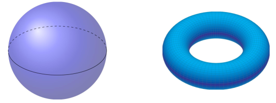
Figure 1: Illustration of a sphere (left) and torus (right).

We consider the case when the (persistent) Betti numbers are built on the alpha complex. The alpha complex is similar, in nature, to the Čech complex (see Example 3.7), but it has a more natural geometric realization. Given a finite set ${\mathcal{X}}$ of points in ${\mathbb{R}}^{d}$ and $r\in[0,\infty]$, the alpha complex $\alpha({\mathcal{X}},r)$ is defined as a collection of subsets $\sigma\subset{\mathcal{X}}$ such that $\bigcap_{x\in\sigma}\big{(}B(x,r/2)\cap V_{x}\big{)}\neq\emptyset$, where $V_{x}$ is a Voronoi cell of $x$; that is, $V_{x}=\big{\{}y\in{\mathbb{R}}^{d}\mathrel{\mathop{\mathchar 58\relax}}\|y-x\|\leq\inf_{z\in{\mathcal{X}}}\|y-z\|\}$. Clearly, it holds that $\alpha({\mathcal{X}},r)\subset\check{C}({\mathcal{X}},r)$. Moreover, we have inclusions $\alpha({\mathcal{X}},r)\subset\alpha({\mathcal{X}},r^{\prime})$ for all $r\leq r^{\prime}$, which indicates that $\alpha({\mathcal{X}},r)$ is a subcomplex of the Delaunay complex $\text{Del}({\mathcal{X}})\mathrel{\mathop{\mathchar 58\relax}}=\alpha({\mathcal{X}},\infty)$. This property plays a crucial role in our analysis; see Remark 4.2.

Returning to the setup in Section 2, we consider the filtration induced by a collection of alpha complexes over a scaled Poisson point process $r_{n}^{-1}\mathcal{P}_{n}$,

$$\big{(}\alpha(r_{n}^{-1}\mathcal{P}_{n},t),\,t\geq 0\big{)}=\big{(}\alpha(\mathcal{P}_{n},r_{n}t),\,t\geq 0\big{)}.$$ (4.1)

Topological changes in the filtration (4.1) can be captured by the $k$th persistent Betti number $\beta_{k,n}(s,t)$ for $0\leq s\leq t\leq\infty$. Loosely speaking, $\beta_{k,n}(s,t)$ represents the number of $k$-cycles, that appear in (4.1) before time $r_{n}s$ and remain alive at time $r_{n}t$. More formally, $\beta_{k,n}(s,t)$ is defined as

$$\beta_{k,n}(s,t)=\text{dim}\frac{Z_{k}\big{(}\alpha(\mathcal{P}_{n},r_{n}s)\big{)}}{Z_{k}\big{(}\alpha(\mathcal{P}_{n},r_{n}s)\big{)}\cap B_{k}\big{(}\alpha(\mathcal{P}_{n},r_{n}t)\big{)}},$$

where $Z_{k}(\cdot)$ is the $k$th cycle group of an alpha complex and $B_{k}(\cdot)$ denotes its $k$th boundary group. Here, the homology coefficients are taken from an arbitrary field. In the special case $s=t$, $\beta_{k,n}(s,t)$ reduces to the ordinary $k$th Betti number.

As mentioned before, in the following we restrict ourselves to a lower-dimensional case $d=2$ and $k=3$ (in the notation of Section 2). For $(x_{1},x_{2},x_{3})\in({\mathbb{R}}^{2})^{3}$ and $r>0$, define

$$h_{r}(x_{1},x_{2}, x_{3})\mathrel{\mathop{\mathchar 58\relax}}={\mathbbm{1}}\Big{\{}\beta_{1}\big{(}\alpha(\{x_{1},x_{2},x_{3}\},r)\big{)}=1\Big{\}}$$ (4.2)

$$={\mathbbm{1}}\bigg{\{}\Big{\{}\bigcap_{j=1,\,j\neq j_{0}}^{3}B(x_{j},r/2)\neq\emptyset\ \text{for all }j_{0}\in\{1,2,3\}\Big{\}}\cap\Big{\{}\bigcap_{j=1}^{3}B(x_{j},r/2)=\emptyset\Big{\}}\bigg{\}}.$$

For a subset ${\mathcal{Y}}$ of $3$ points in ${\mathbb{R}}^{2}$, a finite set $\mathcal{Z}\supset{\mathcal{Y}}$ in ${\mathbb{R}}^{2}$, and $0\leq s\leq t<\infty$,

$$g_{r_{n}s,r_{n}t}({\mathcal{Y}},\mathcal{Z}) \mathrel{\mathop{\mathchar 58\relax}}=h_{r_{n}s}({\mathcal{Y}})\,h_{r_{n}t}({\mathcal{Y}})\,{\mathbbm{1}}\big{\{}\|y-z\|\geq r_{n}t,\text{ for all }y\in{\mathcal{Y}}\text{ and }z\in\mathcal{Z}\setminus{\mathcal{Y}}\big{\}}$$

$$=h_{r_{n}s}({\mathcal{Y}})\,h_{r_{n}t}({\mathcal{Y}})\,{\mathbbm{1}}\big{\{}\alpha({\mathcal{Y}},r_{n}t)\text{ is a connected component of }\alpha(\mathcal{Z},r_{n}t)\big{\}}.$$

Note that $g_{r_{n}s,r_{n}t}({\mathcal{Y}},\mathcal{Z})=1$ if and only if a set ${\mathcal{Y}}$ in ${\mathbb{R}}^{2}$ with $|{\mathcal{Y}}|=3$ forms a single $1$-cycle before time $r_{n}s$, such that this $1$-cycle remains alive at time $r_{n}t$ and isolated from all the remaining points in $\mathcal{Z}$ at that time. The proof of the next theorem is presented in Section 5.4.

Theorem 4.1.

Assume that $\rho_{3,n}\to\infty$ and $nr_{n}^{2}\to 0$ as $n\to\infty$. Then, for every $0\leq s_{i}\leq t_{i}<\infty$, $i=1,\dots,m$, with $(s_{i},t_{i})\neq(s_{j},t_{j})$ for $i\neq j$, and $A\in\mathcal{D}$,

$$\frac{1}{\rho_{3,n}}\log\mathbb{P}\Big{(}\big{(}\rho_{3,n}^{-1}\beta_{1,n}(s_{i},t_{i}),\,i=1,\dots,m\big{)}\in A\Big{)}\to-\inf_{{\bf x}\in A}I_{3}({\bf x}),\ \ \text{as }n\to\infty,$$ (4.3)

where $I_{3}$ is the rate function from (3.10). The unique minimizer of $I_{3}$ equals $(\mu_{1},\dots,\mu_{m})$, where

$$\mu_{i}=\frac{1}{6}\,\int_{({\mathbb{R}}^{2})^{2}}h_{s_{i}}({\bf 0}_{2},{\bf y})\,h_{t_{i}}({\bf 0}_{2},{\bf y})\operatorname{d\!}{\bf y},\ \ i=1,\dots,m,$$

with ${\bf 0}_{2}=(0,0)\in{\mathbb{R}}^{2}$ and ${\bf y}\in({\mathbb{R}}^{2})^{2}$.
Moreover, define $\beta_{1,n}^{\mathsf{B}}(s,t)$ to be the first-order persistent Betti number generated by the binomial point process. Then, $(\beta_{1,n}^{\mathsf{B}})_{n\geq 1}$ satisfies the same LDP as (4.3).

Remark 4.2 (Extensions to higher-dimensions).

In the proof of Theorem 4.1, we shall exploit the Morse inequality, which enables to bound the first-order persistent Betti number by the number of $1$-simplex counts (i.e., edge counts). A key property for dealing with the corresponding exponential moments is that the $1$-simplex count in the planar Delaunay triangulation grows at most linearly in the number of vertices (see Equ. (5.47) for details). Unfortunately, this property breaks down in higher-dimensions ([2]); this is the reason why our discussion must be restricted to a special case $d=2$, $k=3$. Notice, however, that one needs this assumption only for showing (5.47); the rest of our analyses holds true for general $d$ and $k$. For the LDP of higher-order persistent Betti numbers in a higher-dimensional space, we need to develop a new machinery that does not rely on the Morse inequality. More concretely, we need to detect the parameters $d$ and $k$, such that the (persistent) Betti number grows at most linearly in the number of vertices.

4.2 Morse critical points of min-type distance functions

The objective of this example is to deduce the LDP for the number of Morse critical points of a certain min-type distance function. The behavior of Morse critical points of such distance functions have been intensively investigated in the context of central limit theorems and the Poisson process approximation [6, 8, 9, 38]. In addition to its intrinsic interests, this concept has served as a practical quantifier of homological changes in random geometric complexes, especially in the field of Topological Data Analysis ([6, 7]).

Once again, we treat only the special case $d=2$ and $k=3$ (in the notation of Section 2). Given a homogeneous Poisson point process $\mathcal{P}_{n}$ on $[0,1]^{2}$ with intensity $n$, we define min-type distance functions by

$$d_{\mathcal{P}_{n}}(x)\mathrel{\mathop{\mathchar 58\relax}}=\min_{y\in\mathcal{P}_{n}}\|x-y\|,\ \ \ x\in{\mathbb{R}}^{2}.$$

Though $d_{\mathcal{P}_{n}}$ is not differentiable, one can still define the notion of Morse critical points in the following sense. A point $c\in{\mathbb{R}}^{2}$ is said to be a Morse critical point of $d_{\mathcal{P}_{n}}$ with index $2$ if there exists a subset ${\mathcal{Y}}\subset\mathcal{P}_{n}$ of three points such that

$(i)$ The points in ${\mathcal{Y}}$ are in general position.
$(ii)$ $d_{\mathcal{P}_{n}}(c)=\|c-y\|$ for all $y\in{\mathcal{Y}}$ and $d_{\mathcal{P}_{n}}(c)<\min_{z\in\mathcal{P}_{n}\setminus{\mathcal{Y}}}\|c-z\|$.
$(iii)$ The interior of the convex hull spanned by the points in ${\mathcal{Y}}$, denoted $\text{conv}^{\circ}({\mathcal{Y}})$, contains $c$.

By the Nerve theorem (see, e.g., Theorem 10.7 in [4]), for each $r>0$ the sublevel set $d_{\mathcal{P}_{n}}(-\infty,r]$ is homotopy equivalent to a Čech complex $\check{C}(\mathcal{P}_{n},2r)$. For this reason, the number of critical points of $d_{\mathcal{P}_{n}}$ with index $2$ whose critical values are less than $r_{n}$, behaves very similarly to the first-order Betti number of $\check{C}(\mathcal{P}_{n},2r_{n})$ (see [6]). A similar analysis was conducted for the case that distributions are supported on a closed manifold embedded in the ambient Euclidean space [8]. Moreover, [38] studied the case when random points are sampled from a stationary point process.

Given a point set ${\mathcal{Y}}\subset{\mathbb{R}}^{2}$ with $|{\mathcal{Y}}|=3$ in general position, let $\gamma({\mathcal{Y}})$ be the center of a unique $1$-dimensional sphere containing ${\mathcal{Y}}$, and define $\mathcal{R}({\mathcal{Y}})=d_{\mathcal{P}_{n}}\big{(}\gamma({\mathcal{Y}})\big{)}$. If $\gamma({\mathcal{Y}})$ gives a critical point of $d_{\mathcal{P}_{n}}$ (with index $2$), then $\mathcal{R}({\mathcal{Y}})$ represents its critical value. Additionally, $\mathcal{U}({\mathcal{Y}})$ denotes an open ball in ${\mathbb{R}}^{2}$ with radius $\mathcal{R}({\mathcal{Y}})$ centered at $\gamma({\mathcal{Y}})$. Given $t_{i}\in[0,\infty)$, $i=1,\dots,m$, with $t_{i}\neq t_{j}$ for $i\neq j$, we define

$$N_{n}\mathrel{\mathop{\mathchar 58\relax}}=\Big{(}\sum_{{\mathcal{Y}}\subset\mathcal{P}_{n},\,|{\mathcal{Y}}|=3}{\mathbbm{1}}\big{\{}\gamma({\mathcal{Y}})\in\text{conv}^{\circ}({\mathcal{Y}}),\ \mathcal{R}({\mathcal{Y}})\leq r_{n}t_{i},\ \mathcal{U}({\mathcal{Y}})\cap\mathcal{P}_{n}=\emptyset\big{\}}\Big{)}_{i=1}^{m}.$$ (4.4)

In particular, the $i$th entry of $N_{n}$ represents the number of Morse critical points of index $2$ with critical values less than or equal to $r_{n}t_{i}$.

The result below is essentially a consequence of Theorem 3.3 and Proposition 3.5. Unlike Theorem 4.1, we do not provide the result for the version of binomial point processes; the required extension actually involves more complicated machinery. A formal proof is given in Section 5.4.

Theorem 4.3.

Assume that $\rho_{3,n}\to\infty$ and $nr_{n}^{2}\to 0$ as $n\to\infty$. Then, for every measurable $A\in\mathcal{D}$,

$$\frac{1}{\rho_{3,n}}\,\log\mathbb{P}\big{(}\rho_{3,n}^{-1}N_{n}\in A\big{)}\to-\inf_{{\bf x}\in A}I_{3}({\bf x}),\ \ \text{as }n\to\infty,$$

where $I_{3}$ is the rate function from (3.10). The unique minimizer of $I_{3}$ equals $(\mu_{1},\dots,\mu_{m})$, where

$$\mu_{i}=\frac{1}{6}\,\int_{({\mathbb{R}}^{2})^{2}}{\mathbbm{1}}\big{\{}\gamma({\bf 0}_{2},{\bf y})\in\text{conv}^{\circ}({\bf 0}_{2},{\bf y}),\,\mathcal{R}({\bf 0}_{2},{\bf y})\leq t_{i}\big{\}}\operatorname{d\!}{\bf y},\ \ i=1,\dots,m,$$

with ${\bf y}\in({\mathbb{R}}^{2})^{2}$.

5 Proofs

As preparation, we partition the unit cube $[0,1]^{d}$ into $\rho_{k,n}$ sub-cubes $Q_{1},\dots,Q_{\rho_{k,n}}$ of volume $\rho_{k,n}^{-1}$. To avoid notational complication we assume that $\rho_{k,n}$ takes only positive integers for all $n\in{\mathbb{N}}$. This assumption applies to many of the sequences and functions throughout this section. In particular, we set $Q_{1}=[0,\rho_{k,n}^{-1/d}]^{d}$. Given a finite set ${\mathcal{Y}}$ of $k$ points in ${\mathbb{R}}^{d}$, we take $\ell({\mathcal{Y}})$ to be the left most point of ${\mathcal{Y}}$ in the lexicographic ordering. As discussed in Section 2, one may set $\ell({\mathcal{Y}})$ to be a center of the unique $(k-2)$-dimensional sphere containing ${\mathcal{Y}}$. In this case, however, the description will be slightly more involved. Hence, for ease of description, we prefer to define $\ell({\mathcal{Y}})$ as the left most point.

In the below, $C^{*}$ denotes a generic constant, which is independent of $n$ and may vary between and within the lines.

5.1 Proofs of Theorem 2.1, Proposition 2.2, and Corollary 2.3

The proof of Theorem 2.1 can be completed via Propositions 5.1 and 5.6 below. Proposition 5.1 is aimed to give the LDP for

$$\eta_{k,n}=\frac{1}{\rho_{k,n}}\sum_{\ell=1}^{\rho_{k,n}}\sum_{{\mathcal{Y}}\subset\mathcal{P}_{n}|_{Q_{\ell}},\,|{\mathcal{Y}}|=k}s_{n}({\mathcal{Y}},\mathcal{P}_{n}|_{Q_{\ell}};t)\,\delta_{r_{n}^{-1}\overline{\mathcal{Y}}}=\mathrel{\mathop{\mathchar 58\relax}}\frac{1}{\rho_{k,n}}\sum_{\ell=1}^{\rho_{k,n}}\eta_{k,n}^{(\ell)}\in M_{+}(E),$$ (5.1)

where $\mathcal{P}_{n}|_{Q_{\ell}}$ denotes the restriction of $\mathcal{P}_{n}$ to the cube $Q_{\ell}$. Setting up a “blocked” point process as in (5.1) is a standard approach in the literature ([36, 35]). The process (5.1) is of course different from the original process $(\xi_{k,n})_{n\geq 1}$. In fact, if geometric/topological objects exist spreading over multiple cubes in $(Q_{\ell})_{\ell\geq 1}$, then these objects are counted possibly by $(\xi_{k,n})_{n\geq 1}$, whereas they are never counted by $(\eta_{k,n})_{n\geq 1}$. Despite such a difference, one may justify in Proposition 5.6 that the difference between $(\xi_{k,n})_{n\geq 1}$ and $(\eta_{k,n})_{n\geq 1}$ is exponentially negligible in terms of the total variation distance. By virtue of this proposition, as well as Theorem 4.2.13 in [14], our task can be reduced to prove the LDP for $(\eta_{k,n})_{n\geq 1}$.

The main benefit of working with $(\eta_{k,n})_{n\geq 1}$ is that it breaks down into a collection of i.i.d. point processes $(\eta_{k,n}^{(\ell)})_{\ell\geq 1}$. Note that $(\eta_{k,n}^{(\ell)})_{\ell\geq 1}$ are defined in the space $M_{p}(E)$ of finite point measures on $E$. We here equip $M_{p}(E)$ with a Borel $\sigma$-field $\mathcal{M}_{p}(E)\mathrel{\mathop{\mathchar 58\relax}}=\mathcal{M}_{+}(E)\cap M_{p}(E)$. Because of this decomposition, one can clarify the correspondence between (5.1) and the process

$$\zeta_{k,n}\mathrel{\mathop{\mathchar 58\relax}}=\frac{1}{\rho_{k,n}}\sum_{\ell=1}^{\rho_{k,n}}\zeta_{k}^{(\ell)}\in M_{+}(E),\ \ \ n=1,2,\dots,$$ (5.2)

where $(\zeta_{k}^{(\ell)})_{\ell\geq 1}$ are i.i.d. Poisson random measures on $E$ with intensity measure $\tau_{k}$. Write $(\Omega^{\prime},\mathcal{F}^{\prime},\mathbb{P}^{\prime})$ for the probability space on which (5.2) is defined, and $\mathbb{E}^{\prime}$ denotes the corresponding expectation.

In Lemma 5.2 below, we first prove that (5.2) satisfies the required LDP in Theorem 2.1. After that, Lemmas 5.3 and 5.5 are aimed to establish exponential equivalence between (5.1) and (5.2). Now, we formally state one of the main results of this section.

Proposition 5.1.

The sequence $(\eta_{k,n})_{n\geq 1}$ fulfills an LDP in the weak topology with rate $\rho_{k,n}$ and the rate function $\Lambda_{k}^{*}$ in (2.5).

Since the proof of Proposition 5.1 is rather long, we divide it into several lemmas. Combining these lemmas can conclude Proposition 5.1.

Lemma 5.2.

The sequence $(\zeta_{k,n})_{n\geq 1}$ satisfies an LDP in the weak topology with rate $\rho_{k,n}$ and rate function $\Lambda_{k}^{*}$.

Proof.

It follows from Theorem 5.1 in [34] that for every $f\in C_{b}(E)$,

$$\Lambda_{k}(f) \mathrel{\mathop{\mathchar 58\relax}}=\log\mathbb{E}^{\prime}\Big{[}e^{\zeta_{k}^{(1)}(f)}\Big{]}=\frac{1}{k!}\int_{({\mathbb{R}}^{d})^{k-1}}\big{(}e^{f(\overline{({\bf 0}_{d},{\bf y})})}-1\big{)}\,{\mathbbm{1}}\big{\{}\mathsf{diam}({\bf 0}_{d},{\bf y})\leq L\big{\}}\operatorname{d\!}{\bf y}.$$

According to Cramér’s theorem in Polish spaces in [14, Theorem 6.1.3] (see also [14, Corollary 6.2.3]), it turns out that $(\zeta_{k,n})_{n\geq 1}$ satisfies a weak LDP in $M_{+}(E)$ with rate function $\Lambda_{k}^{*}$.

In order to extend this to a full LDP, we need to demonstrate that $(\zeta_{k,n})_{n\geq 1}$ is exponentially tight in the space $M_{+}(E)$. The proof is analogous to that in Lemma 6.2.6 of [14]. Since $\tau_{k}$ is tight in the space $E$, for every $\ell\geq 1$ there exists a compact subset $\Gamma_{\ell}\subset E$, such that $\tau_{k}(E\setminus\Gamma_{\ell})\leq\ell/(e^{2\ell^{2}}-1)$. Define

$$K_{\ell}\mathrel{\mathop{\mathchar 58\relax}}=\big{\{}\nu\in M_{+}(E)\mathrel{\mathop{\mathchar 58\relax}}\nu(E\setminus\Gamma_{\ell})\leq\ell^{-1},\,\nu(E)\leq\ell\big{\}}.$$

By Portmanteau’s theorem for weak convergence, one can deduce that $K_{\ell}$ is weakly closed in $M_{+}(E)$. For $m\geq 1$, let $L_{m}\mathrel{\mathop{\mathchar 58\relax}}=\bigcap_{\ell=m}^{\infty}K_{\ell}$. Obviously, $L_{m}$ is weakly closed in $M_{+}(E)$. Furthermore, Prohorov’s theorem (see, e.g., Theorem A2.4.I in [12]) ensures that $L_{m}$ is relatively compact. Since $L_{m}$ is now compact in $M_{+}(E)$, the exponential tightness of $(\zeta_{k,n})_{n\geq 1}$ follows from

$$\limsup_{n\to\infty}\frac{1}{\rho_{k,n}}\log\mathbb{P}^{\prime}\big{(}\zeta_{k,n}\in M_{+}(E)\setminus L_{m}\big{)}\leq-\big{(}m-\tau_{k}(E)(e-1)\big{)},$$ (5.3)

for every $m\geq 1$. By the union bound,

$$\mathbb{P}^{\prime}\big{(}\zeta_{k,n}\in M_{+}(E)\setminus L_{m}\big{)}\leq\sum_{\ell=m}^{\infty}\Big{\{}\mathbb{P}^{\prime}\big{(}\zeta_{k,n}(E\setminus\Gamma_{\ell})>\ell^{-1}\big{)}+\mathbb{P}^{\prime}\big{(}\zeta_{k,n}(E)>\ell\big{)}\Big{\}}.$$

By Markov’s inequality and the fact that $\zeta_{k}^{(1)}(E\setminus\Gamma_{\ell})$ is Poisson distributed with mean $\tau_{k}(E\setminus\Gamma_{\ell})$,

$$\sum_{\ell=m}^{\infty}\mathbb{P}^{\prime}\big{(}\zeta_{k,n}(E\setminus\Gamma_{\ell})>\ell^{-1}\big{)}\leq\sum_{\ell=m}^{\infty}e^{-2\rho_{k,n}\ell}\Big{(}\mathbb{E}^{\prime}\big{[}e^{2\ell^{2}\zeta_{k}^{(1)}(E\setminus\Gamma_{\ell})}\big{]}\Big{)}^{\rho_{k,n}}$$ (5.4)

$$=\sum_{\ell=m}^{\infty}e^{-2\rho_{k,n}\ell+\rho_{k,n}\tau_{k}(E\setminus\Gamma_{\ell})(e^{2\ell^{2}}-1)}\leq\sum_{\ell=m}^{\infty}e^{-\rho_{k,n}\ell}\leq 2e^{-\rho_{k,n}m}.$$

By the similar calculation,

$$\sum_{\ell=m}^{\infty}\mathbb{P}^{\prime}\big{(}\zeta_{k,n}(E)>\ell\big{)}\leq 2e^{-(m-\tau_{k}(E)(e-1))\rho_{k,n}}.$$ (5.5)

Putting (5.4) and (5.5) together gives (5.3), as desired. ∎

By virtue of Lemma 5.2, our goal is now to show that $(\eta_{k,n})_{n\geq 1}$ in (5.1) satisfies the same LDP as $(\zeta_{k,n})_{n\geq 1}$. As a first step, we claim that for every $\ell\geq 1$, the total variation distance between the laws of $\eta_{k,n}^{(\ell)}$ and $\zeta_{k}^{(\ell)}$ tends to $0$ as $n\to\infty$. Write $\mathcal{L}(\xi)$ for the probability law of a random element $\xi$.

Lemma 5.3.

For every $\ell\geq 1$,

$$d_{\mathsf{TV}}\big{(}\mathcal{L}(\eta_{k,n}^{(\ell)}),\mathcal{L}(\zeta_{k}^{(\ell)})\big{)}\mathrel{\mathop{\mathchar 58\relax}}=\sup_{A\in\mathcal{M}_{p}(E)}\big{|}\mathbb{P}(\eta_{k,n}^{(\ell)}\in A)-\mathbb{P}^{\prime}(\zeta_{k}^{(\ell)}\in A)\big{|}\to 0,\ \ \text{as }n\to\infty.$$ (5.6)

Remark 5.4.

One of the possible extensions of Lemma 5.3 seems to consider the case, for which $(r_{n})_{n\geq 1}$ belongs to the critical regime, i.e., $nr_{n}^{d}\to c\in(0,\infty)$ as $n\to\infty$. In this case, however, the asymptotic behaviors of (5.1) and (5.7) below are essentially different. More concretely, in the critical regime (5.10) no longer holds, since the last term in (5.11) does not vanish as $n\to\infty$.

Proof.

We begin with defining a sequence of random measures,

$$\widetilde{\eta}_{k,n}=\frac{1}{\rho_{k,n}}\sum_{\ell=1}^{\rho_{k,n}}\sum_{{\mathcal{Y}}\subset\mathcal{P}_{n}|_{Q_{\ell}},\,|{\mathcal{Y}}|=k}{\mathbbm{1}}\big{\{}\mathsf{diam}({\mathcal{Y}})\leq r_{n}L\big{\}}\,\delta_{r_{n}^{-1}\overline{\mathcal{Y}}}=\mathrel{\mathop{\mathchar 58\relax}}\frac{1}{\rho_{k,n}}\sum_{\ell=1}^{\rho_{k,n}}\widetilde{\eta}_{k,n}^{(\ell)},\ \ \ n\geq 1.$$ (5.7)

Note that $(\widetilde{\eta}_{k,n}^{(\ell)})_{\ell\geq 1}$ are i.i.d. point processes in the space $M_{p}(E)$. We first show that

$$d_{\mathsf{TV}}\big{(}\mathcal{L}(\widetilde{\eta}_{k,n}^{(\ell)}),\mathcal{L}(\zeta_{k}^{(\ell)})\big{)}\to 0,\ \ \text{as }n\to\infty.$$ (5.8)

According to Theorem 3.1 in [13], (5.8) follows if one can verify that

$$\sup_{A\mathrel{\mathop{\mathchar 58\relax}}\text{Borel in }E}\Big{|}\mathbb{E}\big{[}\widetilde{\eta}_{k,n}^{(\ell)}(A)\big{]}-\mathbb{E}^{\prime}\big{[}\zeta^{(\ell)}_{k}(A)\big{]}\Big{|}\to 0,\ \ \ n\to\infty,$$

and

$$\gamma_{n} \mathrel{\mathop{\mathchar 58\relax}}=\max_{1\leq p\leq k-1}n^{2k-p}\int_{(Q_{\ell})^{2k-p}}{\mathbbm{1}}\big{\{}\mathsf{diam}(x_{1},\dots,x_{k})\leq r_{n}L\big{\}}$$ (5.9)

$$\qquad\qquad\qquad\qquad\times{\mathbbm{1}}\big{\{}\mathsf{diam}(x_{1},\dots,x_{p},x_{k+1},\dots,x_{2k-p})\leq r_{n}L\big{\}}\operatorname{d\!}{\bf x}\to 0,\ \ n\to\infty.$$

By the multivariate Mecke formula for Poisson point processes (see, e.g., Chapter 4 in [23]),

$$\mathbb{E}\big{[}\widetilde{\eta}_{k,n}^{(\ell)}(A)\big{]}=\frac{n^{k}}{k!}\,\int_{(Q_{\ell})^{k}}{\mathbbm{1}}\big{\{}\mathsf{diam}(x_{1},\dots,x_{k})\leq r_{n}L,\ r_{n}^{-1}\overline{(x_{1},\dots,x_{k})}\in A\big{\}}\operatorname{d\!}{\bf x}.$$

Performing the change of variables $x_{i}=x+r_{n}y_{i-1}$, $i=1,\dots,k$ (with $y_{0}\equiv 0$),

$$\mathbb{E}\big{[}\widetilde{\eta}_{k,n}^{(\ell)}(A)\big{]} =\frac{\rho_{k,n}}{k!}\,\int_{Q_{\ell}}\int_{({\mathbb{R}}^{d})^{k-1}}{\mathbbm{1}}\big{\{}\mathsf{diam}({\bf 0}_{d},{\bf y})\leq L,\,\overline{({\bf 0}_{d},{\bf y})}\in A\big{\}}$$

$$\qquad\qquad\qquad\qquad\times\prod_{i=1}^{k-1}{\mathbbm{1}}\{x+r_{n}y_{i}\in Q_{\ell}\}\operatorname{d\!}{\bf y}\operatorname{d\!}x.$$

On the other hand,

$$\mathbb{E}^{\prime}\big{[}\zeta^{(\ell)}_{k}(A)\big{]}=\tau_{k}(A)=\frac{\rho_{k,n}}{k!}\,\int_{Q_{\ell}}\int_{({\mathbb{R}}^{d})^{k-1}}{\mathbbm{1}}\big{\{}\mathsf{diam}({\bf 0}_{d},{\bf y})\leq L,\ \overline{({\bf 0}_{d},{\bf y})}\in A\big{\}}\operatorname{d\!}{\bf y}\operatorname{d\!}x.$$

Thus, as $n\to\infty$,

$$\sup_{A}\Big{|}\mathbb{E}\big{[}\widetilde{\eta}_{k,n}^{(\ell)}(A)\big{]}-\mathbb{E}^{\prime}\big{[}\zeta^{(\ell)}_{k}(A)\big{]}\Big{|} \leq\frac{\rho_{k,n}}{k!}\,\int_{Q_{\ell}}\int_{({\mathbb{R}}^{d})^{k-1}}{\mathbbm{1}}\big{\{}\mathsf{diam}({\bf 0}_{d},{\bf y})\leq L\big{\}}$$

$$\qquad\qquad\times\Big{(}1-\prod_{i=1}^{k-1}{\mathbbm{1}}\{x+r_{n}y_{i}\in Q_{\ell}\}\Big{)}\operatorname{d\!}{\bf y}\operatorname{d\!}x\to 0.$$

As for (5.9), the change of variables $x_{i}=x+r_{n}y_{i-1}$, $i=1,\dots,2k-p$ (with $y_{0}\equiv 0$), yields that

$$\gamma_{n} \mathrel{\mathop{\mathchar 58\relax}}=\max_{1\leq p\leq k-1}n^{2k-p}r_{n}^{d(2k-p-1)}\int_{Q_{\ell}}\int_{({\mathbb{R}}^{d})^{2k-p-1}}{\mathbbm{1}}\big{\{}\mathsf{diam}({\bf 0}_{d},y_{1},\dots,y_{k-1})\leq L\big{\}}$$

$$\qquad\times{\mathbbm{1}}\big{\{}\mathsf{diam}({\bf 0}_{d},y_{1},\dots,y_{p-1},y_{k},\dots,y_{2k-p-1})\leq L\big{\}}\prod_{i=1}^{2k-p-1}{\mathbbm{1}}\{x+r_{n}y_{i}\in Q_{\ell}\}\operatorname{d\!}{\bf y}\operatorname{d\!}x$$

$$\leq\max_{1\leq p\leq k-1}(nr_{n}^{d})^{k-p}\int_{({\mathbb{R}}^{d})^{2k-p-1}}\prod_{i=1}^{2k-p-1}{\mathbbm{1}}\big{\{}\|y_{i}\|\leq L\big{\}}\operatorname{d\!}{\bf y}\to 0,\ \ \ n\to\infty.$$

Thus, (5.8) has been established, and it remains to verify that

$$d_{\mathsf{TV}}\big{(}\mathcal{L}(\widetilde{\eta}_{k,n}^{(\ell)}),\mathcal{L}(\eta_{k,n}^{(\ell)})\big{)}\to 0,\ \ \ n\to\infty.$$ (5.10)

Noting that $\widetilde{\eta}_{k,n}^{(\ell)}$ and $\eta_{k,n}^{(\ell)}$ are both defined in the same probability space, we have

$$d_{\mathsf{TV}}\big{(}\mathcal{L}(\widetilde{\eta}_{k,n}^{(\ell)}),\mathcal{L}(\eta_{k,n}^{(\ell)})\big{)}=\frac{1}{2}\sup_{\|f\|_{\infty}\leq 1}\Big{|}\mathbb{E}\big{[}f(\widetilde{\eta}_{k,n}^{(\ell)})\big{]}-\mathbb{E}\big{[}f(\eta_{k,n}^{(\ell)})\big{]}\Big{|},$$

where the supremum is taken over all $f\mathrel{\mathop{\mathchar 58\relax}}M_{p}(E)\to{\mathbb{R}}$ with $\|f\|_{\infty}\mathrel{\mathop{\mathchar 58\relax}}=\text{esssup}_{x\in M_{p}(E)}|f(x)|\leq 1$. Whenever $f(\widetilde{\eta}_{k,n}^{(\ell)})-f(\eta_{k,n}^{(\ell)})$ is non-zero, there exists a subset ${\mathcal{Y}}$ of $k$ points in $\mathcal{P}_{n}|_{Q_{\ell}}$, such that $\mathsf{diam}({\mathcal{Y}})\leq r_{n}L$ and $c_{n}({\mathcal{Y}},\mathcal{P}_{n}|_{Q_{\ell}};t)=0$. This implies that

$$d_{\mathsf{TV}}\big{(}\mathcal{L}(\widetilde{\eta}_{k,n}^{(\ell)}),\mathcal{L}(\eta_{k,n}^{(\ell)})\big{)} \leq\frac{1}{2}\sup_{\|f\|_{\infty}\leq 1}\mathbb{E}\bigg{[}\,\big{|}\,f(\widetilde{\eta}_{k,n}^{(\ell)})-f(\eta_{k,n}^{(\ell)})\,\big{|}$$

$$\qquad\times{\mathbbm{1}}\bigg{\{}\bigcup_{{\mathcal{Y}}\subset\mathcal{P}_{n}|_{Q_{\ell}}}\Big{\{}\mathsf{diam}({\mathcal{Y}})\leq r_{n}L,\,c_{n}({\mathcal{Y}},\mathcal{P}_{n}|_{Q_{\ell}};t)=0\Big{\}}\bigg{\}}\bigg{]}$$

$$\leq\mathbb{E}\bigg{[}\sum_{{\mathcal{Y}}\subset\mathcal{P}_{n}|_{Q_{\ell}}}{\mathbbm{1}}\big{\{}\mathsf{diam}({\mathcal{Y}})\leq r_{n}L\big{\}}\,\big{(}1-c_{n}({\mathcal{Y}},\mathcal{P}_{n}|_{Q_{\ell}};t)\big{)}\bigg{]}.$$

Writing $\mathcal{B}\big{(}\{x_{1},\dots,x_{k}\};r\big{)}\mathrel{\mathop{\mathchar 58\relax}}=\bigcup_{i=1}^{k}B(x_{i},r)$ and appealing to the Mecke formula for Poisson point processes, the rightmost term above is equal to

$$\begin{split}&\frac{n^{k}}{k!}\int_{(Q_{\ell})^{k}}{\mathbbm{1}}\big{\{}\mathsf{diam}(x_{1},\dots,x_{k})\leq r_{n}L\big{\}}\Big{(}1-e^{-n\text{vol}\big{(}\mathcal{B}(\{x_{1},\dots,x_{k}\};r_{n}t)\cap Q_{\ell}\big{)}}\Big{)}\operatorname{d\!}{\bf x}\\ &=\frac{\rho_{k,n}}{k!}\int_{Q_{\ell}}\int_{({\mathbb{R}}^{d})^{k-1}}{\mathbbm{1}}\big{\{}\mathsf{diam}({\bf 0}_{d},{\bf y})\leq L\big{\}}\prod_{i=1}^{k-1}{\mathbbm{1}}\{x+r_{n}y_{i}\in Q_{\ell}\}\\ &\qquad\qquad\qquad\times\Big{(}1-e^{-n\text{vol}\big{(}\mathcal{B}(\{x,x+r_{n}y_{1},\dots,x+r_{n}y_{k-1}\};r_{n}t)\cap Q_{\ell}\big{)}}\Big{)}\operatorname{d\!}{\bf y}\operatorname{d\!}x\\ &\leq\frac{1}{k!}\int_{({\mathbb{R}}^{d})^{k-1}}{\mathbbm{1}}\big{\{}\mathsf{diam}({\bf 0}_{d},{\bf y})\leq L\big{\}}\Big{(}1-e^{-nr_{n}^{d}\text{vol}\big{(}\mathcal{B}(\{{\bf 0}_{d},{\bf y}\};t)\big{)}}\Big{)}\operatorname{d\!}{\bf y}.\end{split}$$ (5.11)

Since $nr_{n}^{d}\to 0$ as $n\to\infty$, the last integral tends to $0$ as $n\to\infty$. Now, (5.10) is obtained and the proof of (5.6) is completed. ∎

By the standard argument on the maximal coupling (see [21, Lemma 4.32]), for every $\ell\geq 1$, there exists a coupling $(\hat{\eta}_{k,n}^{(\ell)},\hat{\zeta}^{(\ell)}_{k})$ on some probability space $(\hat{\Omega}_{\ell},\hat{\mathcal{F}}_{\ell},\hat{\mathbb{P}}_{\ell})$, such that $\hat{\eta}_{k,n}^{(\ell)}\stackrel{{\scriptstyle d}}{{=}}\eta_{k,n}^{(\ell)}$, $\hat{\zeta}^{(\ell)}_{k}\stackrel{{\scriptstyle d}}{{=}}\zeta^{(\ell)}_{k}$, and

$$\hat{\mathbb{P}}_{\ell}\big{(}\hat{\eta}_{k,n}^{(\ell)}\neq\hat{\zeta}^{(\ell)}_{k}\big{)}=d_{\mathsf{TV}}\big{(}\mathcal{L}(\eta_{k,n}^{(\ell)}),\mathcal{L}(\zeta_{k}^{(\ell)})\big{)}\to 0,\ \ \ n\to\infty,$$ (5.12)

where the last convergence follows from Lemma 5.3. Define $\hat{\Omega}=\prod_{\ell=1}^{\infty}\hat{\Omega}_{\ell}$, $\hat{\mathcal{F}}=\bigotimes_{\ell=1}^{\infty}\hat{\mathcal{F}}_{\ell}$, $\hat{\mathbb{P}}=\bigotimes_{\ell=1}^{\infty}\hat{\mathbb{P}}_{\ell}$, and $\hat{\mathbb{E}}$ is the corresponding expectation; then $(\hat{\eta}_{k,n}^{(\ell)},\hat{\zeta}^{(\ell)}_{k})_{\ell\geq 1}$ becomes a sequence of i.i.d. random vectors under $\hat{\mathbb{P}}$. Define $\hat{\eta}_{k,n}$ and $\hat{\zeta}_{k,n}$ analogously to (5.1) and (5.2).

According to [14, Theorem 4.2.13], if one can show that $(\hat{\eta}_{k,n})_{n\geq 1}$ and $(\hat{\zeta}_{k,n})_{n\geq 1}$ are exponentially equivalent under a coupled probability $\hat{\mathbb{P}}$ (in terms of the total variation distance), then it will be concluded that $(\eta_{k,n})_{n\geq 1}$ and $(\zeta_{k,n})_{n\geq 1}$ exhibit the same LDP. A more precise statement is given as follows.

Lemma 5.5.

For every $\delta>0$,

$$\lim_{n\to\infty}\frac{1}{\rho_{k,n}}\log\hat{\mathbb{P}}\Big{(}d_{\mathsf{TV}}\big{(}\hat{\eta}_{k,n},\hat{\zeta}_{k,n}\big{)}\geq\delta\Big{)}=-\infty.$$ (5.13)

Proof.

By Markov’s inequality, we have, for any $a>0$,

$$\hat{\mathbb{P}}\Big{(}d_{\mathsf{TV}}\big{(}\hat{\eta}_{k,n},\hat{\zeta}_{k,n}\big{)}\geq\delta\Big{)} \leq\hat{\mathbb{P}}\Big{(}\sum_{\ell=1}^{\rho_{k,n}}d_{\mathsf{TV}}\big{(}\hat{\eta}_{k,n}^{(\ell)},\hat{\zeta}^{(\ell)}_{k}\big{)}\geq\delta\rho_{k,n}\Big{)}$$

$$\leq e^{-a\delta\rho_{k,n}}\Big{(}\hat{\mathbb{E}}\Big{[}e^{ad_{\mathsf{TV}}\big{(}\hat{\eta}_{k,n}^{(1)},\,\hat{\zeta}_{k}^{(1)}\big{)}}\Big{]}\Big{)}^{\rho_{k,n}}.$$

Hence, (5.13) follows if we can show that, for every $a>0$,

$$\lim_{n\to\infty}\hat{\mathbb{E}}\Big{[}e^{ad_{\mathsf{TV}}\big{(}\hat{\eta}_{k,n}^{(1)},\,\hat{\zeta}_{k}^{(1)}\big{)}}\Big{]}=1.$$ (5.14)

Because of (5.12), we get that $d_{\mathsf{TV}}\big{(}\hat{\eta}_{k,n}^{(1)},\,\hat{\zeta}_{k}^{(1)}\big{)}\stackrel{{\scriptstyle\hat{\mathbb{P}}}}{{\to}}0$ as $n\to\infty$. It thus remains to demonstrate that

$$\limsup_{n\to\infty}\hat{\mathbb{E}}\Big{[}e^{ad_{\mathsf{TV}}\big{(}\hat{\eta}_{k,n}^{(1)},\,\hat{\zeta}_{k}^{(1)}\big{)}}\Big{]}<\infty,\ \ \text{ for all }a>0.$$ (5.15)

In fact, (5.15) ensures the uniform integrability for the convergence (5.14). By the Cauchy–Schwarz inequality,

$$\hat{\mathbb{E}}\Big{[}e^{ad_{\mathsf{TV}}\big{(}\hat{\eta}_{k,n}^{(1)},\,\hat{\zeta}_{k}^{(1)}\big{)}}\Big{]} \leq\Big{\{}\mathbb{E}\Big{[}e^{2a\eta_{k,n}^{(1)}(E)}\Big{]}\Big{\}}^{1/2}\Big{\{}\mathbb{E}^{\prime}\Big{[}e^{2a\zeta_{k}^{(1)}(E)}\Big{]}\Big{\}}^{1/2}$$

$$=\Big{\{}\mathbb{E}\big{[}e^{2a\sum_{{\mathcal{Y}}\subset\mathcal{P}_{n}|_{Q_{1}}}s_{n}({\mathcal{Y}},\mathcal{P}_{n}|_{Q_{1}};t)}\big{]}\Big{\}}^{1/2}\Big{\{}\exp\big{\{}\tau_{k}(E)(e^{2a}-1)\big{\}}\Big{\}}^{1/2}.$$

Now we need to verify that for all $a>0$,

$$\limsup_{n\to\infty}\mathbb{E}\Big{[}e^{a\sum_{{\mathcal{Y}}\subset\mathcal{P}_{n}|_{Q_{1}}}s_{n}({\mathcal{Y}},\mathcal{P}_{n}|_{Q_{1}};t)}\Big{]}<\infty.$$ (5.16)

For the proof of (5.16), we consider the diluted family of cubes

$$G\mathrel{\mathop{\mathchar 58\relax}}=\big{\{}4Lr_{n}z+[0,tr_{n}/\sqrt{d}]^{d}\subset Q_{1}\mathrel{\mathop{\mathchar 58\relax}}z\in{\mathbb{Z}}^{d}\big{\}}$$ (5.17)

(recall that we have taken $L>t$). Then, $Q_{1}$ can be covered by at most $(4L\sqrt{d}/t)^{d}$ many translates of $G$. Denote these translates as $G_{1},\dots,G_{(4L\sqrt{d}/t)^{d}}$ (with $G_{1}\equiv G$). Let $b_{n}\mathrel{\mathop{\mathchar 58\relax}}=\rho_{k,n}^{-1}/(4Lr_{n})^{d}$ denote the number of cubes (of side length $tr_{n}/\sqrt{d}$) that are contained in $G$. As mentioned at the beginning of Section 5, we assume, without loss of generality, that $(4L\sqrt{d}/t)^{d}$ and $b_{n}$ take only positive integers. Suppose ${\mathcal{Y}}$ is a set of $k$ points with $\mathsf{diam}({\mathcal{Y}})\leq r_{n}L$, then there is a unique $j\in\{1,\dots,(4L\sqrt{d}/t)^{d}\}$, so that the left most point $\ell({\mathcal{Y}})$ belongs to one of the cubes in $G_{j}$. Hence,

$$\sum_{{\mathcal{Y}}\subset\mathcal{P}_{n}|_{Q_{1}}}s_{n}\big{(}{\mathcal{Y}},\mathcal{P}_{n}|_{Q_{1}};t\big{)}=\sum_{j=1}^{(4L\sqrt{d}/t)^{d}}\sum_{{\mathcal{Y}}\subset\mathcal{P}_{n}|_{Q_{1}}}s_{n}\big{(}{\mathcal{Y}},\mathcal{P}_{n}|_{Q_{1}};t\big{)}{\mathbbm{1}}\Big{\{}\ell({\mathcal{Y}})\in\bigcup_{J\in G_{j}}J\Big{\}}.$$ (5.18)

Write $G_{1}=\{J_{1},\dots,J_{b_{n}}\}$ with $J_{1}=\big{[}0,tr_{n}/\sqrt{d}\big{]}^{d}$. By (5.18), Hölder’s inequality, and the spatial independence and homogeneity of $\mathcal{P}_{n}$, we need to demonstrate that

$$\limsup_{n\to\infty}\bigg{(}\mathbb{E}\Big{[}e^{a\sum_{{\mathcal{Y}}\subset\mathcal{P}_{n}|_{Q_{1}}}s_{n}({\mathcal{Y}},\mathcal{P}_{n}|_{Q_{1}};t){\mathbbm{1}}\{\ell({\mathcal{Y}})\in J_{1}\}}\Big{]}\bigg{)}^{b_{n}}<\infty.$$ (5.19)

A key observation for the proof of (5.19) is that there is at most a single $k$-point subset ${\mathcal{Y}}\subset\mathcal{P}_{n}|_{Q_{1}}$ such that $c_{n}({\mathcal{Y}},\mathcal{P}_{n}|_{Q_{1}};t)=1$ and $\ell({\mathcal{Y}})\in J_{1}$. In fact, if there are two distinct point sets ${\mathcal{Y}},{\mathcal{Y}}^{\prime}\subset\mathcal{P}_{n}|_{Q_{1}}$ with $\ell({\mathcal{Y}})\in J_{1}$ and $\ell({\mathcal{Y}}^{\prime})\in J_{1}$, then it must be that $c_{n}({\mathcal{Y}},\mathcal{P}_{n}|_{Q_{1}};t)=c_{n}({\mathcal{Y}}^{\prime},\mathcal{P}_{n}|_{Q_{1}};t)=0$. It turns out from this observation that

$$\sum_{{\mathcal{Y}}\subset\mathcal{P}_{n}|_{Q_{1}}}s_{n}\big{(}{\mathcal{Y}},\mathcal{P}_{n}|_{Q_{1}};t\big{)}{\mathbbm{1}}\big{\{}\ell({\mathcal{Y}})\in J_{1}\big{\}}$$

is a $\{0,1\}$-valued random variable; hence,

$$\bigg{(}\mathbb{E}\Big{[}e^{a\sum_{{\mathcal{Y}}\subset\mathcal{P}_{n}|_{Q_{1}}}s_{n}({\mathcal{Y}},\mathcal{P}_{n}|_{Q_{1}};t){\mathbbm{1}}\{\ell({\mathcal{Y}})\in J_{1}\}}\Big{]}\bigg{)}^{b_{n}}$$

$$=\bigg{(}1+(e^{a}-1)\mathbb{P}\Big{(}\sum_{{\mathcal{Y}}\subset\mathcal{P}_{n}|_{Q_{1}}}s_{n}\big{(}{\mathcal{Y}},\mathcal{P}_{n}|_{Q_{1}};t\big{)}{\mathbbm{1}}\big{\{}\ell({\mathcal{Y}})\in J_{1}\big{\}}=1\Big{)}\bigg{)}^{b_{n}}$$

$$\leq\bigg{(}1+(e^{a}-1)\mathbb{E}\Big{[}\sum_{{\mathcal{Y}}\subset\mathcal{P}_{n}}{\mathbbm{1}}\big{\{}\mathsf{diam}({\mathcal{Y}})\leq r_{n}L,\,\ell({\mathcal{Y}})\in J_{1}\big{\}}\Big{]}\bigg{)}^{b_{n}}.$$

Repeating the same calculations as before, it is not hard to see that

$$\mathbb{E}\Big{[}\sum_{{\mathcal{Y}}\subset\mathcal{P}_{n}}{\mathbbm{1}}\big{\{}\mathsf{diam}({\mathcal{Y}})\leq r_{n}L,\,\ell({\mathcal{Y}})\in J_{1}\big{\}}\Big{]}=C^{*}\big{(}\rho_{k,n}r_{n}^{d}+o(1)\big{)}.$$

Now, we obtain

$$\bigg{(}1+(e^{a}-1)\mathbb{E}\Big{[}\sum_{{\mathcal{Y}}\subset\mathcal{P}_{n}}{\mathbbm{1}}\big{\{}\mathsf{diam}({\mathcal{Y}})\leq r_{n}L,\,\ell({\mathcal{Y}})\in J_{1}\big{\}}\Big{]}\bigg{)}^{b_{n}}\to e^{C^{*}(e^{a}-1)/(4L)^{d}}<\infty,$$

as desired. ∎

Now that the proof of Proposition 5.1 has been completed, we next verify that the difference between $(\xi_{k,n})_{n\geq 1}$ and $(\eta_{k,n})_{n\geq 1}$ in terms of the total variation distance, is exponentially negligible.

Proposition 5.6.

For every $\delta>0$,

$$\lim_{n\to\infty}\frac{1}{\rho_{k,n}}\log\mathbb{P}\big{(}d_{\mathsf{TV}}(\xi_{k,n},\eta_{k,n})\geq\delta\big{)}=-\infty.$$ (5.20)

Proof.

For $\ell=1,\dots,\rho_{k,n}$, define a collection of points in $Q_{\ell}$ that are distance at most $r$ from the boundary of $Q_{\ell}$:

$$Q^{\partial}_{\ell}(r)\mathrel{\mathop{\mathchar 58\relax}}=\big{\{}x\in Q_{\ell}\mathrel{\mathop{\mathchar 58\relax}}\inf_{y\in\partial Q_{\ell}}\|x-y\|\leq r\big{\}},\ \ \ r>0.$$

For a subset $A\subset E$, we discuss two distinct cases for which a $k$-point set ${\mathcal{Y}}\subset[0,1]^{d}$ with $\mathsf{diam}({\mathcal{Y}})\leq r_{n}L$, makes different contributions to $\xi_{k,n}(A)$ and $\eta_{k,n}(A)$. The first case is that the point set ${\mathcal{Y}}$ “crosses a boundary” between two neighboring sub-cubes, i.e., there exist distinct $\ell_{1}$ and $\ell_{2}$ such that

$${\mathcal{Y}}\cap Q_{\ell_{1}}\neq\emptyset,\ \ \ {\mathcal{Y}}\cap Q_{\ell_{2}}\neq\emptyset.$$

Then, ${\mathcal{Y}}$ must be contained in $\bigcup_{\ell=1}^{\rho_{k,n}}Q^{\partial}_{\ell}\big{(}(L+t)r_{n}\big{)}$ such that ${\mathcal{Y}}\cap\bigcup_{\ell=1}^{\rho_{k,n}}Q_{\ell}^{\partial}(tr_{n})\neq\emptyset$. Furthermore, ${\mathcal{Y}}$ may increase the value of $\xi_{k,n}(A)$, while the value of $\eta_{k,n}(A)$ is unchanged. The second case is that there are two neighboring sub-cubes $Q_{\ell_{1}}$ and $Q_{\ell_{2}}$, together with two point sets ${\mathcal{Y}}_{i}\subset Q_{\ell_{i}}$, $i=1,2$, of cardinality $k$ with $\mathsf{diam}({\mathcal{Y}}_{i})\leq r_{n}L$, such that $\inf_{y_{i}\in{\mathcal{Y}}_{i},\,i=1,2}\|y_{1}-y_{2}\|\leq r_{n}t$. It then holds that ${\mathcal{Y}}_{i}\subset Q^{\partial}_{\ell_{i}}\big{(}(L+t)r_{n}\big{)}$ with ${\mathcal{Y}}_{i}\cap Q_{\ell}^{\partial}(tr_{n})\neq\emptyset$ for $i=1,2$. Moreover, ${\mathcal{Y}}_{i}$ may increase the value of $\eta_{k,n}(A)$, but the value of $\xi_{k,n}(A)$ is unchanged. Putting these observations together, we conclude that

$$d_{\mathsf{TV}}(\xi_{k,n},\eta_{k,n}) \leq\frac{1}{\rho_{k,n}}\sum_{{\mathcal{Y}}\subset\mathcal{P}_{n}}s_{n}\big{(}{\mathcal{Y}},\mathcal{P}_{n}|_{\bigcup_{\ell=1}^{\rho_{k,n}}Q_{\ell}^{\partial}((L+t)r_{n})};t\big{)}{\mathbbm{1}}\Big{\{}{\mathcal{Y}}\cap\bigcup_{\ell=1}^{\rho_{k,n}}Q_{\ell}^{\partial}(tr_{n})\neq\emptyset\Big{\}}$$ (5.21)

$$\qquad\qquad+\frac{1}{\rho_{k,n}}\sum_{\ell=1}^{\rho_{k,n}}\sum_{{\mathcal{Y}}\subset\mathcal{P}_{n}}s_{n}\big{(}{\mathcal{Y}},\mathcal{P}_{n}|_{Q^{\partial}_{\ell}((L+t)r_{n})};t\big{)}{\mathbbm{1}}\big{\{}{\mathcal{Y}}\cap Q_{\ell}^{\partial}(tr_{n})\neq\emptyset\big{\}}.$$

Now, (5.20) will follow if one can show that for every $\delta>0$,

$$\lim_{n\to\infty}\frac{1}{\rho_{k,n}}\,\log\mathbb{P}\Big{(}\sum_{{\mathcal{Y}}\subset\mathcal{P}_{n}}s_{n}\big{(}{\mathcal{Y}},\mathcal{P}_{n}|_{\bigcup_{\ell=1}^{\rho_{k,n}}Q_{\ell}^{\partial}((L+t)r_{n})};t\big{)}$$ (5.22)

$$\qquad\qquad\qquad\qquad\qquad\times{\mathbbm{1}}\Big{\{}{\mathcal{Y}}\cap\bigcup_{\ell=1}^{\rho_{k,n}}Q_{\ell}^{\partial}(tr_{n})\neq\emptyset\Big{\}}\geq\delta\rho_{k,n}\Big{)}=-\infty,$$

and

$$\lim_{n\to\infty}\frac{1}{\rho_{k,n}}\,\log\mathbb{P}\Big{(}\sum_{\ell=1}^{\rho_{k,n}}\sum_{{\mathcal{Y}}\subset\mathcal{P}_{n}}s_{n}\big{(}{\mathcal{Y}},\mathcal{P}_{n}|_{Q^{\partial}_{\ell}((L+t)r_{n})};t\big{)}{\mathbbm{1}}\big{\{}{\mathcal{Y}}\cap Q_{\ell}^{\partial}(tr_{n})\neq\emptyset\big{\}}\geq\delta\rho_{k,n}\Big{)}=-\infty.$$ (5.23)

The proof techniques for (5.22) and (5.23) are similar, so we show only (5.22). To begin, for each $1\leq j\leq d$, denote a collection of ordered $j$-tuples by

$$\mathcal{I}_{j}=\big{\{}{\bm{\ell}}=(\ell_{1},\dots,\ell_{j})\mathrel{\mathop{\mathchar 58\relax}}1\leq\ell_{1}<\dots<\ell_{j}\leq d\big{\}}.$$

For ${\bm{\ell}}=(\ell_{1},\dots,\ell_{j})\in\mathcal{I}_{j}$, we define a collection of disjoint hyper-rectangles by

$$J \mathrel{\mathop{\mathchar 58\relax}}=\bigg{\{}\Big{(}\rho_{k,n}^{-1/d}z+\big{[}0,\rho_{k,n}^{-1/d}\big{]}^{\ell_{1}-1}\times\big{[}-(L+t)r_{n},(L+t)r_{n}\big{]}\times\big{[}0,\rho_{k,n}^{-1/d}\big{]}^{\ell_{2}-\ell_{1}-1}$$ (5.24)

$$\qquad\times\big{[}-(L+t)r_{n},(L+t)r_{n}\big{]}\times\big{[}0,\rho_{k,n}^{-1/d}\big{]}^{\ell_{3}-\ell_{2}-1}\times\dots\times\big{[}-(L+t)r_{n},(L+t)r_{n}\big{]}$$

$$\qquad\times\big{[}0,\rho_{k,n}^{-1/d}\big{]}^{\ell_{j}-\ell_{j-1}-1}\times\big{[}-(L+t)r_{n},(L+t)r_{n}\big{]}\times\big{[}0,\rho_{k,n}^{-1/d}\big{]}^{d-\ell_{j}}\Big{)}\cap[0,1]^{d}\mathrel{\mathop{\mathchar 58\relax}}z\in{\mathbb{Z}}_{+}^{d}\bigg{\}}.$$

By construction, all the rectangles in $J$ are contained in $\bigcup_{\ell=1}^{\rho_{k,n}}Q_{\ell}^{\partial}((L+t)r_{n})$. Moreover, since the number of rectangles in $J$ is $\rho_{k,n}$, one can enumerate $J$ in a way that $J=(I_{p,n}^{\bm{\ell}},\,p=1,\dots,\rho_{k,n})$. Then, one can offer the following bound:

$$\sum_{{\mathcal{Y}}\subset\mathcal{P}_{n}}s_{n}\big{(}{\mathcal{Y}},\mathcal{P}_{n}|_{\bigcup_{\ell=1}^{\rho_{k,n}}Q_{\ell}^{\partial}((L+t)r_{n})};t\big{)}{\mathbbm{1}}\Big{\{}{\mathcal{Y}}\cap\bigcup_{\ell=1}^{\rho_{k,n}}Q_{\ell}^{\partial}(tr_{n})\neq\emptyset\Big{\}}$$ (5.25)

$$\leq\sum_{j=1}^{d}\sum_{{\bm{\ell}}\in\mathcal{I}_{j}}\sum_{p=1}^{\rho_{k,n}}\sum_{{\mathcal{Y}}\subset\mathcal{P}_{n}|_{I_{p,n}^{\bm{\ell}}}}s_{n}\big{(}{\mathcal{Y}},\mathcal{P}_{n}|_{I_{p,n}^{\bm{\ell}}};t\big{)}.$$

Owing to this bound, it remains to show that for every $j\in\{1,\dots,d\}$, ${\bm{\ell}}\in\mathcal{I}_{j}$, and $\delta>0$,

$$\lim_{n\to\infty}\frac{1}{\rho_{k,n}}\,\log\mathbb{P}\Big{(}\sum_{p=1}^{\rho_{k,n}}\sum_{{\mathcal{Y}}\subset\mathcal{P}_{n}|_{I_{p,n}^{\bm{\ell}}}}s_{n}\big{(}{\mathcal{Y}},\mathcal{P}_{n}|_{I_{p,n}^{\bm{\ell}}};t\big{)}\geq\delta\rho_{k,n}\Big{)}=-\infty.$$ (5.26)

Since $(I_{p,n}^{\bm{\ell}},\,p=1,\dots,\rho_{k,n})$ are disjoint, the spatial independence of $\mathcal{P}_{n}$ ensures that

$$\bigg{(}\sum_{{\mathcal{Y}}\subset\mathcal{P}_{n}|_{I_{p,n}^{\bm{\ell}}}}s_{n}\big{(}{\mathcal{Y}},\mathcal{P}_{n}|_{I_{p,n}^{\bm{\ell}}};t\big{)},\,p=1,\dots,\rho_{k,n}\bigg{)}$$

are i.i.d. random variables. Hence, we have for every $a>0$,

$$\mathbb{P}\Big{(}\sum_{p=1}^{\rho_{k,n}}\sum_{{\mathcal{Y}}\subset\mathcal{P}_{n}|_{I_{p,n}^{\bm{\ell}}}}s_{n}\big{(}{\mathcal{Y}},\mathcal{P}_{n}|_{I_{p,n}^{\bm{\ell}}};t\big{)}\geq\delta\rho_{k,n}\Big{)}$$

$$\quad\leq e^{-a\delta\rho_{k,n}}\bigg{(}\mathbb{E}\Big{[}\exp\Big{\{}a\sum_{{\mathcal{Y}}\subset\mathcal{P}_{n}|_{I_{1,n}^{\bm{\ell}}}}s_{n}\big{(}{\mathcal{Y}},\mathcal{P}_{n}|_{I_{1,n}^{\bm{\ell}}};t\big{)}\Big{\}}\Big{]}\bigg{)}^{\rho_{k,n}}.$$

For the proof of (5.26), it is now sufficient to show that for every $a>0$,

$$\mathbb{E}\bigg{[}\exp\Big{\{}a\sum_{{\mathcal{Y}}\subset\mathcal{P}_{n}|_{I_{1,n}^{\bm{\ell}}}}s_{n}\big{(}{\mathcal{Y}},\mathcal{P}_{n}|_{I_{1,n}^{\bm{\ell}}};t\big{)}\Big{\}}\bigg{]}\to 1,\ \ \text{as }n\to\infty.$$ (5.27)

By the same argument as that for (5.16), one can see that for every $a>0$,

$$\limsup_{n\to\infty}\mathbb{E}\bigg{[}\exp\Big{\{}a\sum_{{\mathcal{Y}}\subset\mathcal{P}_{n}|_{I_{1,n}^{\bm{\ell}}}}s_{n}\big{(}{\mathcal{Y}},\mathcal{P}_{n}|_{I_{1,n}^{\bm{\ell}}};t\big{)}\Big{\}}\bigg{]}<\infty,$$

which implies the required uniform integrability. Now, (5.27) will follow if we can verify that

$$\sum_{{\mathcal{Y}}\subset\mathcal{P}_{n}|_{I_{1,n}^{\bm{\ell}}}}s_{n}\big{(}{\mathcal{Y}},\mathcal{P}_{n}|_{I_{1,n}^{\bm{\ell}}};t\big{)}\stackrel{{\scriptstyle\mathbb{P}}}{{\to}}0,\ \ \text{as }n\to\infty.$$ (5.28)

To show this, we have as $n\to\infty$,

$$\mathbb{E}\Big{[}\sum_{{\mathcal{Y}}\subset\mathcal{P}_{n}|_{I_{1,n}^{\bm{\ell}}}}s_{n}\big{(}{\mathcal{Y}},\mathcal{P}_{n}|_{I_{1,n}^{\bm{\ell}}};t\big{)}\Big{]}\leq\mathbb{E}\Big{[}\sum_{{\mathcal{Y}}\subset\mathcal{P}_{n}|_{I_{1,n}^{\bm{\ell}}}}{\mathbbm{1}}\big{\{}\mathsf{diam}({\mathcal{Y}})\leq r_{n}L\big{\}}\Big{]}$$

$$\qquad\qquad=\frac{n^{k}}{k!}\,\int_{(I_{1,n}^{\bm{\ell}})^{k}}{\mathbbm{1}}\big{\{}\mathsf{diam}(x_{1},\dots,x_{k})\leq r_{n}L\big{\}}\operatorname{d\!}{\bf x}$$

$$\qquad\qquad=\frac{\rho_{k,n}}{k!}\,\int_{I_{1,n}^{\bm{\ell}}}\int_{({\mathbb{R}}^{d})^{k-1}}{\mathbbm{1}}\big{\{}\mathsf{diam}({\bf 0}_{d},{\bf y})\leq L\big{\}}\prod_{i=1}^{k-1}{\mathbbm{1}}\big{\{}x+r_{n}y_{i}\in I_{1,n}^{\bm{\ell}}\big{\}}\operatorname{d\!}{\bf y}\operatorname{d\!}x$$

$$\qquad\qquad\leq\frac{\rho_{k,n}}{k!}\,\text{vol}(I_{1,n}^{\bm{\ell}})\int_{({\mathbb{R}}^{d})^{k-1}}{\mathbbm{1}}\big{\{}\mathsf{diam}({\bf 0}_{d},{\bf y})\leq L\big{\}}\operatorname{d\!}{\bf y}=\mathcal{O}\big{(}(nr_{n}^{d})^{k/d}\big{)}\to 0.$$

Hence (5.28) has been established, as desired. ∎

Before concluding this subsection, we present the proof of Proposition 2.2.

Proof of Proposition 2.2.

Our proof is closely related to Theorem 5.4 in [32]. Our goal here is to show that, for every $f\in C_{b}(E)$,

$$\int_{E}\big{(}e^{f({\bf x})}-1\big{)}\tau_{k}(\operatorname{d\!}{\bf x})=\sup_{\rho\in M_{+}(E)}\big{\{}\langle\rho,f\rangle-H_{k}(\rho|\tau_{k})\big{\}},$$ (5.29)

where $\langle\rho,f\rangle\mathrel{\mathop{\mathchar 58\relax}}=\int_{E}f({\bf x})\rho(\operatorname{d\!}{\bf x})$. Given $f\in C_{b}(E)$, we define $\operatorname{d\!}\rho=e^{f}\operatorname{d\!}\tau_{k}$. Then, $\rho\in M_{+}(E)$ with $\rho\ll\tau_{k}$. By (2.7), it is elementary to calculate that $\langle\rho,f\rangle-H_{k}(\rho|\tau_{k})=\int_{E}\big{(}e^{f({\bf x})}-1\big{)}\tau_{k}(\operatorname{d\!}{\bf x})$, which has shown that the left hand side in (5.29) is bounded by the right hand side.

Next, let us take $\nu\in M_{+}(E)$ with $\nu\ll\tau_{k}$, say with density $\varphi$. Then, by Jensen’s inequality,

$$\int_{E}\log\bigg{(}\frac{e^{f({\bf x})}}{\varphi({\bf x})}\bigg{)}\,\frac{\nu(d{\bf x})}{\nu(E)}\leq\log\bigg{(}\int_{E}\frac{e^{f({\bf x})}}{\varphi({\bf x})}\frac{\nu(d{\bf x})}{\nu(E)}\bigg{)}=\log\bigg{(}\int_{E}e^{f({\bf x})}\frac{\tau_{k}(d{\bf x})}{\nu(E)}\bigg{)}.$$

Hence, by (2.7) and the elementary inequality: $1+\log x\leq x$ for $x>0$,

$$\langle\nu,f\rangle-H_{k}(\nu|\tau_{k}){\leq\nu(E)\bigg{\{}1+\log\bigg{(}\int_{E}e^{f({\bf x})}\frac{\tau_{k}(dx)}{\nu(E)}\bigg{)}\bigg{\}}-\tau_{k}(E)}\leq\int_{E}\big{(}e^{f({\bf x})}-1\big{)}\tau_{k}(\operatorname{d\!}{\bf x}).$$

Now (5.29) is obtained, and the rest of the argument after (5.29) is essentially the same as Theorem 5.4 in [32], so we will omit it. ∎

Finally, we prove Corollary 2.3. We can deduce its assertion from Theorem 2.1 by showing that for every $\varepsilon_{0}>0$,

$$\lim_{n\to\infty}\rho_{k,n}^{-1}\log\mathbb{P}\big{(}d_{\mathsf{TV}}(\xi_{k,n},\xi_{k,n}^{\mathsf{B}})\geq\varepsilon_{0}\big{)}=-\infty.$$

Proof of Corollary 2.3.

Similarly as in the proof of Lemma 5.5, we consider a family of diluted cubes. In the current setting, we take

$$G\mathrel{\mathop{\mathchar 58\relax}}=\big{\{}8Lr_{n}z+[0,4Lr_{n}]^{d}\subset[0,1]^{d}\mathrel{\mathop{\mathchar 58\relax}}z\in{\mathbb{Z}}^{d}\big{\}}.$$ (5.30)

Then, $[0,1]^{d}$ can be covered by $2^{d}$ translates of $G$. As before, we write $G=\{J_{1},\dots,J_{b_{n}^{\prime}}\}$ with $J_{1}=\big{[}0,4Lr_{n}\big{]}^{d}$, where $b_{n}^{\prime}\mathrel{\mathop{\mathchar 58\relax}}=(8Lr_{n})^{-d}$ denotes the number of cubes that are contained in $G$. Since there are at most finitely many translates of $G$, it suffices to prove that as $n\to\infty$,

$$\rho_{k,n}^{-1}\log\mathbb{P}\bigg{(}\sup_{A\subset E}\Big{|}\sum_{{\mathcal{Y}}\subset\mathcal{P}_{n},\,|{\mathcal{Y}}|=k}s_{n}({\mathcal{Y}},\mathcal{P}_{n};t){\mathbbm{1}}\Big{\{}\ell({\mathcal{Y}})\in\bigcup_{i=1}^{b_{n}^{\prime}}J_{i}\Big{\}}\,\delta_{r_{n}^{-1}\overline{\mathcal{Y}}}(A)$$

$$\qquad\qquad\qquad-\sum_{{\mathcal{Y}}\subset\mathcal{B}_{n},\,|{\mathcal{Y}}|=k}s_{n}({\mathcal{Y}},\mathcal{B}_{n};t){\mathbbm{1}}\Big{\{}\ell({\mathcal{Y}})\in\bigcup_{i=1}^{b_{n}^{\prime}}J_{i}\Big{\}}\,\delta_{r_{n}^{-1}\overline{\mathcal{Y}}}(A)\Big{|}\geq\varepsilon_{0}\rho_{k,n}\bigg{)}\to-\infty$$

(recall that $\ell({\mathcal{Y}})$ is the left most point of ${\mathcal{Y}}$ in the lexicographic ordering).

We say that $J_{i}$ is an $n$-bad cube if one of the following events happens.

• There exists a $k$-element subset ${\mathcal{Y}}\subset\mathcal{P}_{n}$ with $\ell({\mathcal{Y}})\in J_{i}$, $s_{n}({\mathcal{Y}},\mathcal{P}_{n};t)=1$, such that ${\mathcal{Y}}\not\subset\mathcal{B}_{n}$ or $s_{n}\big{(}{\mathcal{Y}},\mathcal{B}_{n};t\big{)}=0$ holds.

• There exists a $k$-element subset ${\mathcal{Y}}\subset\mathcal{B}_{n}$ with $\ell({\mathcal{Y}})\in J_{i}$, $s_{n}({\mathcal{Y}},\mathcal{B}_{n};t)=1$, such that ${\mathcal{Y}}\not\subset\mathcal{P}_{n}$ or $s_{n}\big{(}{\mathcal{Y}},\mathcal{P}_{n};t\big{)}=0$ holds.

In this setting, the key observation is that there exists a constant $M>0$, such that

$$\sup_{A\subset E}\Big{|}\sum_{{\mathcal{Y}}\subset\mathcal{P}_{n},\,|{\mathcal{Y}}|=k}s_{n}({\mathcal{Y}},\mathcal{P}_{n};t){\mathbbm{1}}\Big{\{}\ell({\mathcal{Y}})\in\bigcup_{i=1}^{b_{n}^{\prime}}J_{i}\Big{\}}\,\delta_{r_{n}^{-1}\overline{\mathcal{Y}}}(A)$$

$$\qquad\qquad\qquad-\sum_{{\mathcal{Y}}\subset\mathcal{B}_{n},\,|{\mathcal{Y}}|=k}s_{n}({\mathcal{Y}},\mathcal{B}_{n};t){\mathbbm{1}}\Big{\{}\ell({\mathcal{Y}})\in\bigcup_{i=1}^{b_{n}^{\prime}}J_{i}\Big{\}}\,\delta_{r_{n}^{-1}\overline{\mathcal{Y}}}(A)\Big{|}$$

$$\leq M\sum_{i=1}^{b_{n}^{\prime}}{\mathbbm{1}}\{J_{i}\text{ is $n$-bad}\}.$$

Thus, it suffices to show that for every $\varepsilon_{0}>0$,

$$\lim_{n\to\infty}\frac{1}{\rho_{k,n}}\log\mathbb{P}\Big{(}\sum_{i=1}^{b_{n}^{\prime}}{\mathbbm{1}}\{J_{i}\text{ is $n$-bad}\}\geq\varepsilon_{0}\rho_{k,n}\Big{)}=-\infty.$$

For $0<\varepsilon\leq 1$, let $\mathcal{P}_{n}^{(\varepsilon)}$ be a homogeneous Poisson point process on $[0,1]^{d}$ with intensity $n\varepsilon$, independent of $\mathcal{P}_{n}$. Then, $\mathcal{P}_{n}^{(\varepsilon,\mathsf{a})}\mathrel{\mathop{\mathchar 58\relax}}=\mathcal{P}_{n}\cup\mathcal{P}_{n}^{(\varepsilon)}$ represents an augmented version of $\mathcal{P}_{n}$ with intensity $n(1+\varepsilon)$. Moreover, $\mathcal{P}_{n}^{(\varepsilon,\mathsf{t})}$ denotes a thinned version of $\mathcal{P}_{n}$, obtained by removing points with probability $\varepsilon$. Notice that $\mathcal{P}_{n}^{(\varepsilon,\mathsf{a})}\stackrel{{\scriptstyle d}}{{=}}\mathcal{P}_{n(1+\varepsilon)}$ and $\mathcal{P}_{n}^{(\varepsilon,\mathsf{t})}\stackrel{{\scriptstyle d}}{{=}}\mathcal{P}_{n(1-\varepsilon)}$. In this setting, we introduce the event

$$F_{n,\varepsilon}\mathrel{\mathop{\mathchar 58\relax}}=\big{\{}\mathcal{P}_{n}^{(\varepsilon,\mathsf{t})}\subset\mathcal{B}_{n}\subset\mathcal{P}_{n}^{(\varepsilon,\mathsf{a})}\big{\}},$$

and note by the Poisson concentration bound from [31, Lemma 1.2],

$$\limsup_{n\to\infty}\rho_{k,n}^{-1}\log\mathbb{P}\big{(}F_{n,\varepsilon}^{c}\big{)}\leq-C^{*}\lim_{n\to\infty}\rho_{k,n}^{-1}n=-\infty.$$ (5.31)

The key advantage of the event $F_{n,\varepsilon}$ is that it allows to simplify the property of being $n$-bad. Indeed, if $J_{i}$ is $n$-bad and $F_{n,\varepsilon}$ holds, then $J_{i}$ becomes $(n,\varepsilon)$-special, in the sense that

$$T\cap(\mathcal{P}_{n}^{(\varepsilon,\mathsf{a})}\setminus\mathcal{P}_{n}^{(\varepsilon,\mathsf{t})})\neq\emptyset,\ \ \text{ and }\ \ \mathcal{P}_{n}^{(\varepsilon,\mathsf{a})}(T)\geq k,$$

where

$$T\mathrel{\mathop{\mathchar 58\relax}}=\big{\{}x\in{\mathbb{R}}^{d}\mathrel{\mathop{\mathchar 58\relax}}\inf_{y\in J_{i}}\|x-y\|\leq 2r_{n}L\big{\}},\ r>0.$$

Since we work with diluted cubes in (5.30), one can see that $\big{(}{\mathbbm{1}}\{J_{i}\text{ is }(n,\varepsilon)\text{-special}\}\big{)}_{i=1}^{b_{n}^{\prime}}$ are i.i.d. Bernoulli random variables. Thus, the number of $(n,\varepsilon)$-special cubes is a binomial random variable with $b_{n}^{\prime}$ trials and success probability $p_{n,\varepsilon}\mathrel{\mathop{\mathchar 58\relax}}=\mathbb{P}\big{(}J_{1}\text{ is $(n,\varepsilon)$-special}\big{)}.$ Then, one can bound $p_{n,\varepsilon}$ as follows:

$$p_{n,\varepsilon} \leq\mathbb{P}\big{(}T\cap(\mathcal{P}_{n}^{(\varepsilon,\mathsf{a})}\setminus\mathcal{P}_{n}^{(\varepsilon,\mathsf{t})})\neq\emptyset\,\big{|}\,\mathcal{P}_{n}^{(\varepsilon,\mathsf{a})}(T)=k\big{)}\mathbb{P}\big{(}\mathcal{P}_{n}^{(\varepsilon,\mathsf{a})}(T)=k\big{)}$$

$$\qquad\qquad\qquad\qquad\qquad\qquad\qquad\qquad+\mathbb{P}\big{(}\mathcal{P}_{n}^{(\varepsilon,\mathsf{a})}(T)\geq k+1\big{)}$$

$$\leq 2k\varepsilon\mathbb{P}\big{(}\mathcal{P}_{n(1+\varepsilon)}(T)=k\big{)}+\mathbb{P}\big{(}\mathcal{P}_{n(1+\varepsilon)}(T)\geq k+1\big{)}$$

$$\leq C^{*}\big{(}\varepsilon(nr_{n}^{d})^{k}+(nr_{n}^{d})^{k+1}\big{)}.$$

In conclusion, if one takes sufficiently small $\varepsilon>0$, then

$$b_{n}^{\prime}p_{n,\varepsilon}\leq C^{*}b_{n}^{\prime}\big{(}\varepsilon(nr_{n}^{d})^{k}+(nr_{n}^{d})^{k+1}\big{)}\leq\varepsilon_{0}\rho_{k,n}$$

for large $n$ enough. Therefore, the binomial concentration inequality [31, Lemma 1.1] gives that

$$\limsup_{n\to\infty}\frac{1}{\rho_{k,n}}\log\mathbb{P}\big{(}\text{Bin}(b_{n}^{\prime},p_{n,\varepsilon})\geq\varepsilon_{0}\rho_{k,n}\big{)} \leq-\lim_{n\to\infty}\frac{\varepsilon_{0}}{2}\,\log\bigg{\{}\frac{\varepsilon_{0}\rho_{k,n}}{C^{*}b_{n}^{\prime}(\varepsilon(nr_{n}^{d})^{k}+(nr_{n}^{d})^{k+1})}\bigg{\}}$$

$$=-\frac{\varepsilon_{0}}{2}\log\Big{\{}\frac{(8L)^{d}\varepsilon_{0}}{C^{*}\varepsilon}\Big{\}}.$$

The last term tends to $-\infty$ as $\varepsilon\to 0$. Hence, combining this result with (5.31) concludes the proof of Corollary 2.3. ∎

5.2 Proofs of Theorem 3.1 and Corollary 3.2

First we point out that the proof of Corollary 3.2 is almost identical to that of Corollary 2.3, so we skip it here. For the proof of Theorem 3.1, we define

$$V_{k,n}\mathrel{\mathop{\mathchar 58\relax}}=\frac{1}{\rho_{k,n}}\sum_{{\mathcal{Y}}\subset\mathcal{P}_{n},\,|{\mathcal{Y}}|=k}s_{n}({\mathcal{Y}},\mathcal{P}_{n};t)\,\delta_{H_{n}({\mathcal{Y}})}\in M_{+}(E^{\prime}).$$

The key step of our proof is to show that the assertions of Theorem 3.1 still hold even when $(U_{k,n})_{n\geq 1}$ is replaced by $(V_{k,n})_{n\geq 1}$. To clarify our presentation, we state this step as a separate proposition.

Proposition 5.7.

The sequence $(V_{k,n})_{n\geq 1}$ satisfies an LDP in the weak topology with rate $\rho_{k,n}$ and the rate function $\bar{\Lambda}_{k}^{*}$ defined in (3.5).

Proof.

The process $(V_{k,n})_{n\geq 1}$ has structure very similar to that of $(\xi_{k,n})_{n\geq 1}$ in (2.4); thus, the proof techniques for Proposition 5.7 are parallel to those for Theorem 2.1. More precisely, as an analog of (5.1), we define

$$W_{k,n}=\frac{1}{\rho_{k,n}}\sum_{\ell=1}^{\rho_{k,n}}\sum_{{\mathcal{Y}}\subset\mathcal{P}_{n}|_{Q_{\ell}},\,|{\mathcal{Y}}|=k}s_{n}({\mathcal{Y}},\mathcal{P}_{n}|_{Q_{\ell}};t)\,\delta_{H_{n}({\mathcal{Y}})}\in M_{+}(E^{\prime}).$$

It then follows from the same argument as Proposition 5.1 that $(W_{k,n})_{n\geq 1}$ satisfies an LDP in the weak topology with rate $\rho_{k,n}$ and the rate function $\bar{\Lambda}_{k}^{*}$. Subsequently, by repeating the proof of Proposition 5.6, one can also establish that for every $\delta>0$,

$$\lim_{n\to\infty}\frac{1}{\rho_{k,n}}\log\mathbb{P}\big{(}d_{\mathsf{TV}}(V_{k,n},W_{k,n})\geq\delta\big{)}=-\infty.$$

This concludes the proof of Proposition 5.7. ∎

Proof of Theorem 3.1.

We now have to show that $(U_{k,n})_{n\geq 1}$ exhibits the same LDP as $(V_{k,n})_{n\geq 1}$ above. We take, without loss of generality, $0<t_{1}\leq t_{2}\leq\dots\leq t_{m}<\infty$ for time parameters of $(U_{k,n})_{n\geq 1}$, whereas we fix the parameter of $(V_{k,n})_{n\geq 1}$ at $t=t_{1}$. In this setup, we need to verity that for every $\delta>0$,

$$\lim_{n\to\infty}\frac{1}{\rho_{k,n}}\log\mathbb{P}\big{(}{d_{\mathsf{TV}}(U_{k,n},V_{k,n})}\geq\delta\big{)}=-\infty.$$

It is straightforward to see that

$${d_{\mathsf{TV}}(U_{k,n},V_{k,n})}\leq\frac{1}{\rho_{k,n}}\sum_{{\mathcal{Y}}\subset\mathcal{P}_{n},\,|{\mathcal{Y}}|=k}s_{n}({\mathcal{Y}},\mathcal{P}_{n};t_{1})\big{(}1-c_{n}({\mathcal{Y}},\mathcal{P}_{n};t_{m})\big{)}.$$

By virtue of the partition of $[0,1]^{d}$ into multiple sub-cubes $Q_{1},\dots,Q_{\rho_{k,n}}$ as in the proof of Proposition 5.1, what need to be shown are

$$\lim_{n\to\infty}\frac{1}{\rho_{k,n}}\log\mathbb{P}\Big{(}\sum_{\ell=1}^{\rho_{k,n}}\sum_{{\mathcal{Y}}\subset\mathcal{P}_{n}|_{Q_{\ell}}}s_{n}({\mathcal{Y}},\mathcal{P}_{n}|_{Q_{\ell}};t_{1})\big{(}1-c_{n}({\mathcal{Y}},\mathcal{P}_{n}|_{Q_{\ell}};t_{m})\big{)}\geq\delta\rho_{k,n}\Big{)}=-\infty,$$ (5.32)

and

$$\lim_{n\to\infty}\frac{1}{\rho_{k,n}}\log\, \mathbb{P}\Big{(}\,\Big{|}\sum_{{\mathcal{Y}}\subset\mathcal{P}_{n}}s_{n}({\mathcal{Y}},\mathcal{P}_{n};t_{1})\big{(}1-c_{n}({\mathcal{Y}},\mathcal{P}_{n};t_{m})\big{)}$$

$$\qquad-\sum_{\ell=1}^{\rho_{k,n}}\sum_{{\mathcal{Y}}\subset\mathcal{P}_{n}|_{Q_{\ell}}}s_{n}({\mathcal{Y}},\mathcal{P}_{n}|_{Q_{\ell}};t_{1})\big{(}1-c_{n}({\mathcal{Y}},\mathcal{P}_{n}|_{Q_{\ell}};t_{m})\big{)}\Big{|}\geq\delta\rho_{k,n}\Big{)}=-\infty,$$

for every $\delta>0$. Of the last two conditions, the latter can be established by the same argument as Proposition 5.6. By Markov’s inequality, (5.32) will follow if we can show that for every $a>0$,

$$\mathbb{E}\Big{[}e^{a\sum_{{\mathcal{Y}}\subset\mathcal{P}_{n}|_{Q_{1}}}s_{n}({\mathcal{Y}},\mathcal{P}_{n}|_{Q_{1}};t_{1})(1-c_{n}({\mathcal{Y}},\mathcal{P}_{n}|_{Q_{1}};t_{m}))}\Big{]}\to 1,\ \ n\to\infty.$$ (5.33)

Repeating the same calculations as in (5.11), while using an obvious bound $s_{n}({\mathcal{Y}},\mathcal{P}_{n}|_{Q_{1}};t_{1})\leq{\mathbbm{1}}\big{\{}\mathsf{diam}({\mathcal{Y}})\leq r_{n}L\big{\}}$, as well as the Mecke formula for Poisson point processes,

$$\mathbb{E}\Big{[}\sum_{{\mathcal{Y}}\subset\mathcal{P}_{n}|_{Q_{1}}}s_{n}({\mathcal{Y}},\mathcal{P}_{n}|_{Q_{1}};t_{1})(1-c_{n}({\mathcal{Y}},\mathcal{P}_{n}|_{Q_{1}};t_{m}))\Big{]}$$

$$\leq\frac{1}{k!}\,\int_{({\mathbb{R}}^{d})^{k-1}}{\mathbbm{1}}\big{\{}\mathsf{diam}({\bf 0}_{d},{\bf y})\leq L\big{\}}\Big{(}1-e^{-nr_{n}^{d}\text{vol}(\mathcal{B}(\{{\bf 0}_{d},{\bf y}\};t_{m}))}\Big{)}\operatorname{d\!}{\bf y}\to 0,\ \ \text{as }n\to\infty.$$

Since we have already shown the uniform integrability by (5.16), we now obtain (5.33), as desired.

Finally, by the same proof as Proposition 2.2, we can obtain (3.6). ∎

5.3 Proofs of Theorem 3.3, Corollary 3.4, and Proposition 3.5

In this section, we first prove Proposition 3.5, because the proof of Theorem 3.3 makes use of Proposition 3.5.

Proof of Proposition 3.5.

For every ${\bf x}=(x_{1},\dots,x_{m})\in E^{\prime}$, one can choose ${\bf a}=(a_{1},\dots,a_{m})\in{\mathbb{R}}^{m}$ so that

$$u_{i}({\bf x},{\bf a})\mathrel{\mathop{\mathchar 58\relax}}=\frac{1}{k!}\int_{({\mathbb{R}}^{d})^{k-1}}h^{(i)}({\bf 0}_{d},{\bf y})e^{\sum_{r=1}^{m}a_{r}h^{(r)}({\bf 0}_{d},{\bf y})}\operatorname{d\!}{\bf y}-x_{i}=0,\ \ i=1,\dots,m,$$

with ${\bf y}\in({\mathbb{R}}^{d})^{k-1}$. By condition (H4), $u_{i}$ is continuously differentiable with respect to $({\bf x},{\bf a})$. Furthermore, (H5) ensures that the matrix $\big{(}\partial u_{i}/\partial a_{j}\big{)}_{i,j=1}^{m}$ is positive definite. Thus, by the implicit function theorem, there exist continuously differentiable functions $\alpha_{r}\mathrel{\mathop{\mathchar 58\relax}}E^{\prime}\to{\mathbb{R}}$, $r=1,\dots,m$, such that

$$I_{k}({\bf x})=\sum_{i=1}^{m}\alpha_{i}({\bf x})x_{i}-\frac{1}{k!}\,\int_{({\mathbb{R}}^{d})^{k-1}}\Big{(}e^{\sum_{i=1}^{m}\alpha_{i}({\bf x})h^{(i)}({\bf 0}_{d},{\bf y})}-1\Big{)}\operatorname{d\!}{\bf y},$$ (5.34)

and

$$x_{i}=\frac{1}{k!}\int_{({\mathbb{R}}^{d})^{k-1}}h^{(i)}({\bf 0}_{d},{\bf y})e^{\sum_{r=1}^{m}\alpha_{r}({\bf x})h^{(r)}({\bf 0}_{d},{\bf y})}\operatorname{d\!}{\bf y},\ \ i=1,\dots,m.$$

In particular, (5.34) implies that $I_{k}$ is continuously differentiable on $E^{\prime}$.

For Part $(ii)$, we show that the Hessian of $I_{k}$, denoted $\mathcal{H}(I_{k})$, is positive definite. First it is elementary to check that $\partial I_{k}({\bf x})/\partial x_{j}=\alpha_{j}({\bf x})$ for $j=1,\dots,m$. Using this, it is not hard to calculate that $\mathcal{H}(I_{k})=A^{-1}$ where $A=(A_{ij})$ is given by

$$A_{ij}=\frac{1}{k!}\,\int_{({\mathbb{R}}^{d})^{k-1}}h^{(i)}({\bf 0}_{d},{\bf y})h^{(j)}({\bf 0}_{d},{\bf y})e^{{\sum_{r=1}^{m}\alpha_{r}({\bf x})h^{(r)}({\bf 0}_{d},{\bf y})}}\operatorname{d\!}{\bf y}.$$

We conclude from condition (H5) that $A$ is positive definite; thus, so is $A^{-1}$ as required. Finally, if we set $0=\partial I_{k}({\bf x})/\partial x_{j}$ for every $j=1,\dots,m$, then $\alpha_{j}({\bf x})=0$, and so, $x_{j}=\mu_{j}$ and $I_{k}({\bf x})=0$. As $I_{k}$ is strictly convex, $(\mu_{1},\dots,\mu_{m})$ is a unique minimizer of $I_{k}$. ∎

The proof of Theorem 3.3 is based on an extension of the contraction principle, provided in [14, Theorem 4.2.23]. We begin with defining a map $F\mathrel{\mathop{\mathchar 58\relax}}M_{+}(E^{\prime})\to[0,\infty)^{m}$ by $F(\rho)=\big{(}\int_{E^{\prime}}x_{i}\rho(\operatorname{d\!}{\bf x})\big{)}_{i=1}^{m}$. Then, $F(U_{k,n})=T_{k,n}/\rho_{k,n}$, where $U_{k,n}$ and $T_{k,n}$ are defined in (3.4) and (3.8), respectively. Since $F$ is not continuous in the weak topology, we need to introduce a family of continuous maps: $F_{K}(\rho)\mathrel{\mathop{\mathchar 58\relax}}=\big{(}\int_{E^{\prime}}s_{i}^{(K)}({\bf x})\rho(\operatorname{d\!}{\bf x})\big{)}_{i=1}^{m}$, where

$$s_{i}^{(K)}(x_{1},\dots,x_{m})=\begin{cases}x_{i}&\text{ if }0\leq x_{i}\leq K,\\ -K^{2}(x_{i}-K)+K&\text{ if }K\leq x_{i}\leq K+K^{-1},\\ 0&\text{ if }x_{i}\geq K+K^{-1}.\end{cases}$$

Clearly, $s_{i}^{(K)}$ is continuous and bounded on $E^{\prime}$, and consequently, $F_{K}$ becomes continuous in the weak topology.

In order to apply [14, Theorem 4.2.23], we need to demonstrate the following auxiliary results.

Lemma 5.8.

$(i)$ Let $\delta>0$. Then,

$$\limsup_{K\to\infty}\limsup_{n\to\infty}\frac{1}{\rho_{k,n}}\log\mathbb{P}\Big{(}\big{\|}F(U_{k,n})-F_{K}(U_{k,n})\big{\|}>\delta\Big{)}=-\infty,$$

$(ii)$ Let $a>0$. Then,

$$\limsup_{K\to\infty}\sup_{\rho\in M_{+}(E^{\prime}),\,\bar{\Lambda}_{k}^{*}(\rho)\leq a}\big{\|}F(\rho)-F_{K}(\rho)\big{\|}=0.$$

Assuming the assertions of Lemma 5.8 temporarily, we first explain how to conclude the proof of Theorem 3.3.

Proof of Theorem 3.3.

Note that one can conclude from Theorem 3.1, [14, Theorem 4.2.23], and Lemma 5.8 that $(T_{k,n}/\rho_{k,n})_{n\geq 1}$ satisfies an LDP with rate $\rho_{k,n}$ and the rate function

$$\inf_{\nu\in M_{+}(E^{\prime}),\,F(\nu)={\bf x}}H_{k}^{\prime}(\nu|\tau_{k}^{\prime}),\ \ \ {\bf x}\in{\mathbb{R}}^{m},$$

where $H_{k}^{\prime}$ is a relative entropy given at (3.7). It thus remains to show that

$$\inf_{\nu\in M_{+}(E^{\prime}),\,F(\nu)={\bf x}}H_{k}^{\prime}(\nu|\tau_{k}^{\prime})=I_{k}({\bf x}),\ \ \ {\bf x}\in{\mathbb{R}}^{m}.$$ (5.35)

If $x_{i}<0$ for some $i\in\{1,\dots,m\}$, both sides above are equal to infinity. So from onward, we consider ${\bf x}\in E^{\prime}$ and prove first that $\inf_{\nu\in M_{+}(E^{\prime}),\,F(\nu)={\bf x}}H_{k}^{\prime}(\nu|\tau_{k}^{\prime})\geq I_{k}({\bf x})$. Fix $\nu\in M_{+}(E^{\prime})$ such that $F(\nu)={\bf x}$. For every ${\bf a}\in{\mathbb{R}}^{m}$, we set $f({\bf z})=\langle{\bf a},{\bf z}\rangle$ for ${\bf z}\in E^{\prime}$. Approximating $f$ via a sequence of continuous and bounded functions, we have

$$H_{k}^{\prime}(\nu|\tau_{k}^{\prime}) =\bar{\Lambda}_{k}^{*}(\nu)\geq\langle\nu,f\rangle-\frac{1}{k!}\int_{({\mathbb{R}}^{d})^{k-1}}\big{(}e^{f(H({\bf 0}_{d},{\bf y}))}-1\big{)}\,{\mathbbm{1}}\big{\{}H({\bf 0}_{d},{\bf y})\neq{\bf 0}_{m}\big{\}}\operatorname{d\!}{\bf y}$$

$$=\langle{\bf a},{\bf x}\rangle-\frac{1}{k!}\int_{({\mathbb{R}}^{d})^{k-1}}\big{(}e^{\langle{\bf a},H({\bf 0}_{d},{\bf y})\rangle}-1\big{)}\operatorname{d\!}{\bf y};$$

thus, $H_{k}^{\prime}(\nu|\tau_{k}^{\prime})\geq I_{k}({\bf x})$ holds. Next, for every ${\bf x}\in E^{\prime}$, there exists ${\bf a}_{0}\in{\mathbb{R}}^{m}$ such that

$$I_{k}({\bf x}){=\langle{\bf a}_{0},{\bf x}\rangle-\frac{1}{k!}\int_{({\mathbb{R}}^{d})^{k-1}}\big{(}e^{\langle{\bf a}_{0},H({\bf 0}_{d},{\bf y})\rangle}-1\big{)}\operatorname{d\!}{\bf y}}=\langle{\bf a}_{0},{\bf x}\rangle-\int_{E^{\prime}}\big{(}e^{\langle{\bf a}_{0},{\bf z}\rangle}-1\big{)}\tau_{k}^{\prime}(\operatorname{d\!}{\bf z}),$$

where $x_{i}=\int_{E^{\prime}}z_{i}e^{\langle{\bf a}_{0},{\bf z}\rangle}\tau_{k}^{\prime}(\operatorname{d\!}{\bf z})$ for $i=1,\dots,m$. Define $\nu(A)\mathrel{\mathop{\mathchar 58\relax}}=\int_{A}e^{\langle{\bf a}_{0},{\bf z}\rangle}\tau_{k}^{\prime}(\operatorname{d\!}{\bf z})$, $A\subset E^{\prime}$. It then follows that $\int_{E^{\prime}}z_{i}\nu(\operatorname{d\!}{\bf z})=x_{i}$ for $i=1,\dots,m$; equivalently, $F(\nu)={\bf x}$. Moreover,

$$H_{k}^{\prime}(\nu|\tau_{k}^{\prime})=\int_{E^{\prime}}\log\frac{\operatorname{d\!}\nu}{\operatorname{d\!}\tau_{k}^{\prime}}({\bf z})\nu(\operatorname{d\!}{\bf z})-\nu(E^{\prime})+\tau_{k}^{\prime}(E^{\prime})=\langle{\bf a}_{0},{\bf x}\rangle-\int_{E^{\prime}}\big{(}e^{\langle{\bf a}_{0},{\bf z}\rangle}-1\big{)}\tau_{k}^{\prime}(\operatorname{d\!}{\bf z})=I_{k}({\bf x}).$$

This implies $\inf_{\nu\in M_{+}(E^{\prime}),\,F(\nu)={\bf x}}H_{k}^{\prime}(\nu|\tau_{k}^{\prime})\leq I_{k}({\bf x})$, and thus, the proof of (5.35) has been completed.

Finally, Proposition 3.5 $(i)$ ensures that $I_{k}$ is continuous; therefore, the LDP for $(T_{k,n}/\rho_{k,n})$ implies the convergence in (3.9).

∎

Now, we present the proof of Lemma 5.8.

Proof of Lemma 5.8 $(i)$.

Note first that the result follows from

$$\limsup_{K\to\infty}\limsup_{n\to\infty}\frac{1}{\rho_{k,n}}\log\mathbb{P}\Big{(}\sum_{{\mathcal{Y}}\subset\mathcal{P}_{n}}g_{n}^{(i)}({\mathcal{Y}},\mathcal{P}_{n};t_{i})\,{\mathbbm{1}}\big{\{}h_{n}^{(i)}({\mathcal{Y}})>K\big{\}}\geq\delta\rho_{k,n}\Big{)}=-\infty,$$ (5.36)

for each $i\in\{1,\dots,m\}$. In the sequel, we prefer to use the notation $G_{n}$ and $H_{n}$, instead of $g_{n}^{(i)}$ and $h_{n}^{(i)}$, with the assumption $m=1$, so that the range of $G_{n}$ and $H_{n}$ is $[0,\infty)$. Additionally, we drop the subscript $i$ from $t_{i}$. Then, (5.36) can be rephrased as

$$\limsup_{K\to\infty}\limsup_{n\to\infty}\frac{1}{\rho_{k,n}}\log\mathbb{P}\Big{(}\sum_{{\mathcal{Y}}\subset\mathcal{P}_{n}}G_{n}({\mathcal{Y}},\mathcal{P}_{n};t)\,{\mathbbm{1}}\big{\{}H_{n}({\mathcal{Y}})>K\big{\}}\geq\delta\rho_{k,n}\Big{)}=-\infty.$$ (5.37)

Clearly, (5.37) is implied by

$$\limsup_{K\to\infty}\limsup_{n\to\infty}\frac{1}{\rho_{k,n}}\log\mathbb{P}\Big{(}\sum_{\ell=1}^{\rho_{k,n}}\sum_{{\mathcal{Y}}\subset\mathcal{P}_{n}|_{Q_{\ell}}}G_{n}({\mathcal{Y}},\mathcal{P}_{n}|_{Q_{\ell}};t)\,{\mathbbm{1}}\big{\{}H_{n}({\mathcal{Y}})>K\big{\}}\geq\delta\rho_{k,n}\Big{)}=-\infty,$$ (5.38)

and

$$\limsup_{K\to\infty}\limsup_{n\to\infty}\frac{1}{\rho_{k,n}}\log\mathbb{P}\bigg{(}\,\Big{|}\sum_{{\mathcal{Y}}\subset\mathcal{P}_{n}}G_{n}({\mathcal{Y}},\mathcal{P}_{n};t)\,{\mathbbm{1}}\big{\{}H_{n}({\mathcal{Y}})>K\big{\}}$$ (5.39)

$$\qquad\qquad\qquad\qquad\qquad-\sum_{\ell=1}^{\rho_{k,n}}\sum_{{\mathcal{Y}}\subset\mathcal{P}_{n}|_{Q_{\ell}}}G_{n}({\mathcal{Y}},\mathcal{P}_{n}|_{Q_{\ell}};t)\,{\mathbbm{1}}\big{\{}H_{n}({\mathcal{Y}})>K\big{\}}\Big{|}\geq\delta\rho_{k,n}\bigg{)}=-\infty,$$

for every $\delta>0$. As for (5.38), Markov’s inequality yields that

$$\frac{1}{\rho_{k,n}}\log\mathbb{P}\Big{(}\sum_{\ell=1}^{\rho_{k,n}}\sum_{{\mathcal{Y}}\subset\mathcal{P}_{n}|_{Q_{\ell}}}G_{n}({\mathcal{Y}},\mathcal{P}_{n}|_{Q_{\ell}};t)\,{\mathbbm{1}}\big{\{}H_{n}({\mathcal{Y}})>K\big{\}}\geq\delta\rho_{k,n}\Big{)}$$

$$\leq-a\delta+\log\mathbb{E}\Big{[}e^{a\sum_{{\mathcal{Y}}\subset\mathcal{P}_{n}|_{Q_{1}}}G_{n}({\mathcal{Y}},\mathcal{P}_{n}|_{Q_{1}};t)\,{\mathbbm{1}}\{H_{n}({\mathcal{Y}})>K\}}\Big{]}.$$

It is thus sufficient to demonstrate that for every $a>0$,

$$\limsup_{K\to\infty}\limsup_{n\to\infty}\mathbb{E}\Big{[}e^{a\sum_{{\mathcal{Y}}\subset\mathcal{P}_{n}|_{Q_{1}}}G_{n}({\mathcal{Y}},\mathcal{P}_{n}|_{Q_{1}};t){\mathbbm{1}}\{H_{n}({\mathcal{Y}})>K\}}\Big{]}=1.$$ (5.40)

Although the proof techniques for (5.40) are mostly the same as those for (5.16), we still need to update it because $G_{n}$ in (5.40) is not necessarily an indicator function. Using the same logic as in the proof of (5.16), our goal is to prove that for every $a>0$,

$$\limsup_{K\to\infty}\limsup_{n\to\infty}\bigg{(}\mathbb{E}\Big{[}e^{a\sum_{{\mathcal{Y}}\subset\mathcal{P}_{n}|_{Q_{1}}}G_{n}({\mathcal{Y}},\mathcal{P}_{n}|_{Q_{1}};t){\mathbbm{1}}\{H_{n}({\mathcal{Y}})>K,\,\ell({\mathcal{Y}})\in J_{1}\}}\Big{]}\bigg{)}^{b_{n}}\leq 1,$$

where $J_{1}=\big{[}0,tr_{n}/\sqrt{d}\big{]}^{d}$ and $b_{n}=\rho_{k,n}^{-1}/(4Lr_{n})^{d}$. Observe, once again, that there exists at most a single $k$-point set ${\mathcal{Y}}\subset\mathcal{P}_{n}|_{Q_{1}}$ satisfying $c_{n}({\mathcal{Y}},\mathcal{P}_{n}|_{Q_{1}};t)=1$ and $\ell({\mathcal{Y}})\in J_{1}$. Therefore, as $n\to\infty$,

$$\mathbb{E}\Big{[}e^{a\sum_{{\mathcal{Y}}\subset\mathcal{P}_{n}|_{Q_{1}}}G_{n}({\mathcal{Y}},\mathcal{P}_{n}|_{Q_{1}};t){\mathbbm{1}}\{H_{n}({\mathcal{Y}})>K,\,\ell({\mathcal{Y}})\in J_{1}\}}\Big{]}$$ (5.41)

$$\leq 1+\mathbb{E}\Big{[}\sum_{{\mathcal{Y}}\subset\mathcal{P}_{n}}e^{aH_{n}({\mathcal{Y}})}{\mathbbm{1}}\big{\{}H_{n}({\mathcal{Y}})>K,\,\ell({\mathcal{Y}})\in J_{1}\big{\}}\Big{]}$$

$$=1+\frac{n^{k}}{k!}\int_{([0,1]^{d})^{k}}e^{aH_{n}(x_{1},\dots,x_{k})}{\mathbbm{1}}\big{\{}H_{n}(x_{1},\dots,x_{k})>K,\,\ell(x_{1},\dots,x_{k})\in J_{1}\big{\}}\operatorname{d\!}{\bf x}$$

$$=1+\frac{\rho_{k,n}}{k!}\int_{[0,1]^{d}}\int_{({\mathbb{R}}^{d})^{k-1}}e^{aH({\bf 0}_{d},{\bf y})}{\mathbbm{1}}\big{\{}H({\bf 0}_{d},{\bf y})>K,\,\ell(x,x+r_{n}y_{1},\dots,x+r_{n}y_{k-1})\in J_{1}\big{\}}$$

$$\qquad\qquad\qquad\qquad\qquad\qquad\qquad\qquad\qquad\qquad\times\prod_{i=1}^{k-1}{\mathbbm{1}}\big{\{}x+r_{n}y_{i}\in[0,1]^{d}\big{\}}\operatorname{d\!}{\bf y}\operatorname{d\!}x$$

$$\leq 1+C^{*}\rho_{k,n}r_{n}^{d}\int_{({\mathbb{R}}^{d})^{k-1}}e^{aH({\bf 0}_{d},{\bf y})}{\mathbbm{1}}\big{\{}H({\bf 0}_{d},{\bf y})>K\big{\}}\operatorname{d\!}{\bf y}.$$

Here, the last integral is finite due to property (H4). Now, it follows from (5.41) that

$$\limsup_{K\to\infty}\limsup_{n\to\infty}\bigg{(}\mathbb{E}\Big{[}e^{a\sum_{{\mathcal{Y}}\subset\mathcal{P}_{n}|_{Q_{1}}}G_{n}({\mathcal{Y}},\mathcal{P}_{n}|_{Q_{1}};t){\mathbbm{1}}\{H_{n}({\mathcal{Y}})>K,\,\ell({\mathcal{Y}})\in J_{1}\}}\Big{]}\bigg{)}^{b_{n}}$$

$$\leq\limsup_{K\to\infty}\exp\Big{\{}\frac{C^{*}}{(4L)^{d}}\int_{({\mathbb{R}}^{d})^{k-1}}e^{aH({\bf 0}_{d},{\bf y})}{\mathbbm{1}}\big{\{}H_{n}({\mathcal{Y}})>K\big{\}}\operatorname{d\!}{\bf y}\Big{\}}=1$$

Next, turning to condition (5.39), we deduce an inequality analogous to (5.21):

$$\Big{|}\sum_{{\mathcal{Y}}\subset\mathcal{P}_{n}}G_{n}({\mathcal{Y}},\mathcal{P}_{n};t)\,{\mathbbm{1}}\big{\{}H_{n}({\mathcal{Y}})>K\big{\}}-\sum_{\ell=1}^{\rho_{k,n}}\sum_{{\mathcal{Y}}\subset\mathcal{P}_{n}|_{Q_{\ell}}}G_{n}({\mathcal{Y}},\mathcal{P}_{n}|_{Q_{\ell}};t)\,{\mathbbm{1}}\big{\{}H_{n}({\mathcal{Y}})>K\big{\}}\Big{|}$$

$$\leq\sum_{{\mathcal{Y}}\subset\mathcal{P}_{n}}G_{n}\big{(}{\mathcal{Y}},\mathcal{P}_{n}|_{\bigcup_{\ell=1}^{\rho_{k,n}}Q_{\ell}^{\partial}((L+t)r_{n})};t\big{)}{\mathbbm{1}}\Big{\{}{\mathcal{Y}}\subset\bigcup_{\ell=1}^{\rho_{k,n}}Q_{\ell}^{\partial}\big{(}(L+t)r_{n}\big{)}\Big{\}}$$

$$\qquad\qquad\qquad\qquad\qquad\qquad+\sum_{\ell=1}^{\rho_{k,n}}\sum_{{\mathcal{Y}}\subset\mathcal{P}_{n}|_{Q^{\partial}_{\ell}((L+t)r_{n})}}G_{n}\big{(}{\mathcal{Y}},\mathcal{P}_{n}|_{Q^{\partial}_{\ell}((L+t)r_{n})};t\big{)}.$$

Proceeding the same argument as those after (5.21), while using property (H4), we can get (5.39). Now, the proof of Lemma 5.8 $(i)$ is completed. ∎

Proof of Lemma 5.8 $(ii)$.

Suppose, for contradiction, that we can choose $a>0$ and $\delta>0$ such that

$$\limsup_{K\to\infty}\sup_{\rho\in M_{+}(E^{\prime}),\,\bar{\Lambda}_{k}^{*}(\rho)\leq a}\big{\|}F(\rho)-F_{K}(\rho)\big{\|}>\delta.$$ (5.42)

For $K^{\prime}\geq K+K^{-1}$, define

$$F_{K,K^{\prime}}(\rho)\mathrel{\mathop{\mathchar 58\relax}}=\Big{(}\int_{E^{\prime}}u_{i}^{(K,K^{\prime})}({\bf x})\rho(\operatorname{d\!}{\bf x})\Big{)}_{i=1}^{m},\ \ \ \rho\in M_{+}(E^{\prime}),$$

where

$$u_{i}^{(K,K^{\prime})}(x_{1},\dots,x_{m})=\begin{cases}0&\text{ if }x_{i}\in[0,K]\cup[K^{\prime}+(K^{\prime})^{-1},\infty),\\ (K^{2}+1)(x_{i}-K)&\text{ if }K\leq x_{i}\leq K+K^{-1},\\ x_{i}&\text{ if }K+K^{-1}\leq x_{i}\leq K^{\prime},\\ -(K^{\prime})^{2}(x_{i}-K^{\prime})+K^{\prime}&\text{ if }K^{\prime}\leq x_{i}\leq K^{\prime}+(K^{\prime})^{-1}.\end{cases}$$

Then, $F_{K,K^{\prime}}$ is continuous in the weak topology, and further,

$$\big{\|}F_{K,K^{\prime}}(\rho)\big{\|}\nearrow\big{\|}F(\rho)-F_{K}(\rho)\big{\|},\ \ \text{as }K^{\prime}\uparrow\infty.$$ (5.43)

By Lemma 5.8 $(i)$ and (5.43), we can choose $K_{1}>0$ so that

$$\limsup_{n\to\infty}\frac{1}{\rho_{k,n}}\log\mathbb{P}\Big{(}\big{\|}F_{K,K^{\prime}}(U_{k,n})\big{\|}>\delta\Big{)}<-a$$ (5.44)

for any $K^{\prime}$ and $K$, with $K^{\prime}\geq K+K^{-1}>K\geq K_{1}$. By virtue of the continuity of $F_{K,K^{\prime}}$ together with (5.44), one can apply the contraction principle to the LDP for $(U_{k,n})_{n\geq 1}$ (see Theorem 3.1), to obtain that

$$\inf_{\rho\in M_{+}(E^{\prime}),\,\|F_{K,K^{\prime}}(\rho)\|>\delta}\bar{\Lambda}_{k}^{*}(\rho)>a,$$

for all $K^{\prime}\geq K+K^{-1}>K\geq K_{1}$.

Next, let us turn to (5.42) and fix $K\geq K_{1}$, so that $\sup_{\rho\in M_{+}(E^{\prime}),\,\bar{\Lambda}_{k}^{*}(\rho)\leq a}\big{\|}F(\rho)-F_{K}(\rho)\big{\|}>\delta$. Then, we can choose $\nu\in M_{+}(E^{\prime})$ with $\bar{\Lambda}_{k}^{*}(\nu)\leq a$ and $\big{\|}F(\nu)-F_{K}(\nu)\big{\|}>\delta$. Furthermore, (5.43) implies that there exists $K^{\prime}\geq K+K^{-1}$ with $\big{\|}F_{K,K^{\prime}}(\nu)\big{\|}>\delta$. Since this is contradiction, we have established Lemma 5.8 $(ii)$, as desired. ∎

Finally, we prove Corollary 3.4. The proof is very similar to that of Corollary 2.3. Hence, we focus only on some of its key differences. The goal is to show that for every $\varepsilon_{0}>0$,

$$\lim_{n\to\infty}\rho_{k,n}^{-1}\log\mathbb{P}\big{(}\|T_{k,n}-T_{k,n}^{\mathsf{B}}\|\geq\varepsilon_{0}\rho_{k,n}\big{)}=-\infty.$$

Proof of Corollary 3.4.

As in the proof of Lemma 5.8 $(i)$, we may put the assumption $m=1$ and use the notation $G_{n}$ and $H_{n}$ (instead of $g_{n}^{(1)}$ and $h_{n}^{(1)}$). For $K>0$, we decompose $T_{k,n}^{\mathsf{B}}=T_{\leq K,k,n}^{\mathsf{B}}+T_{>K,k,n}^{\mathsf{B}}$, where

$$T_{\leq K,k,n}^{\mathsf{B}}\mathrel{\mathop{\mathchar 58\relax}}=\sum_{{\mathcal{Y}}\subset\mathcal{B}_{n},\,|{\mathcal{Y}}|=k}G_{n}({\mathcal{Y}},\mathcal{B}_{n};t){\mathbbm{1}}\{H_{n}({\mathcal{Y}})\leq K\},$$

and

$$T_{>K,k,n}^{\mathsf{B}}\mathrel{\mathop{\mathchar 58\relax}}=\sum_{{\mathcal{Y}}\subset\mathcal{B}_{n},\,|{\mathcal{Y}}|=k}G_{n}({\mathcal{Y}},\mathcal{B}_{n};t){\mathbbm{1}}\{H_{n}({\mathcal{Y}})>K\}.$$

Similarly, we write $T_{k,n}=T_{\leq K,k,n}+T_{>K,k,n}$. Since all the summands in $T_{\leq K,k,n}$ and $T_{\leq K,k,n}^{\mathsf{B}}$ are bounded by $K$, a simple repetition of the proof of Corollary 2.3 can yield that

$$\frac{1}{\rho_{k,n}}\log\mathbb{P}\big{(}\,|\,T_{\leq K,k,n}-T_{\leq K,k,n}^{\mathsf{B}}\,|\geq\varepsilon_{0}\rho_{k,n}\big{)}\to-\infty,\ \ \ n\to\infty,$$

for every $K>0$. Additionally, the proof of Lemma 5.8 $(i)$ has already shown that

$$\limsup_{K\to\infty}\limsup_{n\to\infty}\frac{1}{\rho_{k,n}}\log\mathbb{P}(T_{>K,k,n}\geq\varepsilon_{0}\rho_{k,n})=-\infty;$$

so it remains to verify that

$$\limsup_{K\to\infty}\limsup_{n\to\infty}\frac{1}{\rho_{k,n}}\log\mathbb{P}\big{(}T_{>K,k,n}^{\mathsf{B}}\geq\varepsilon_{0}\rho_{k,n}\big{)}=-\infty.$$ (5.45)

Using the same diluted cubes from the proof of Corollary 2.3, (5.45) will follow, provided that

$$\limsup_{K\to\infty}\limsup_{n\to\infty}\frac{1}{\rho_{k,n}}\log\mathbb{P}\Big{(}\sum_{i=1}^{b_{n}^{\prime}}\sum_{{\mathcal{Y}}\subset\mathcal{B}_{n},\,|{\mathcal{Y}}|=k}G_{n}({\mathcal{Y}},\mathcal{B}_{n};t)$$

$$\qquad\qquad\qquad\qquad\qquad\qquad\qquad\times{\mathbbm{1}}\big{\{}H_{n}({\mathcal{Y}})>K,\,\ell({\mathcal{Y}})\in J_{i}\big{\}}\geq\varepsilon_{0}\rho_{k,n}\Big{)}=-\infty.$$

Observe again that there exists a constant $M>0$ such that

$$\begin{split}&\sum_{{\mathcal{Y}}\subset\mathcal{B}_{n},\,|{\mathcal{Y}}|=k}G_{n}({\mathcal{Y}},\mathcal{B}_{n};t){\mathbbm{1}}\{H_{n}({\mathcal{Y}})>K,\,\ell({\mathcal{Y}})\in J_{i}\}\\ &\quad\leq M\max_{{\mathcal{Y}}\subset\mathcal{B}_{n},\,|{\mathcal{Y}}|=k}\Big{(}H_{n}({\mathcal{Y}}){\mathbbm{1}}\{H_{n}({\mathcal{Y}})>K,\,\ell({\mathcal{Y}})\in J_{i}\}\Big{)}.\end{split}$$ (5.46)

Moreover, as in the proof of Corollary 2.3, we may work under the event $\big{\{}\mathcal{B}_{n}\subset\mathcal{P}_{n}^{(1,\mathsf{a})}\big{\}}$, where $\mathcal{P}_{n}^{(1,\mathsf{a})}=\mathcal{P}_{n}\cup\mathcal{P}_{n}^{(1)}\stackrel{{\scriptstyle d}}{{=}}\mathcal{P}_{2n}$. By Markov’s inequality and (5.46), we have, for every $a>0$,

$$\mathbb{P}\Big{(}\Big{\{}\sum_{i=1}^{b_{n}^{\prime}}\sum_{{\mathcal{Y}}\subset\mathcal{B}_{n},\,|{\mathcal{Y}}|=k}G_{n}({\mathcal{Y}},\mathcal{B}_{n};t){\mathbbm{1}}\{H_{n}({\mathcal{Y}})>K,\,\ell({\mathcal{Y}})\in J_{i}\}\geq\varepsilon_{0}\rho_{k,n}\Big{\}}\cap\big{\{}\mathcal{B}_{n}\subset\mathcal{P}_{n}^{(1,\mathsf{a})}\big{\}}\Big{)}$$

$$\quad\leq\mathbb{P}\Big{(}\sum_{i=1}^{b_{n}^{\prime}}M\max_{{\mathcal{Y}}\subset\mathcal{P}_{n}^{(1,\mathsf{a})},\,|{\mathcal{Y}}|=k}\Big{(}H_{n}({\mathcal{Y}}){\mathbbm{1}}\{H_{n}({\mathcal{Y}})>K,\,\ell({\mathcal{Y}})\in J_{i}\}\Big{)}\geq\varepsilon_{0}\rho_{k,n}\Big{)}$$

$$\quad\leq e^{-a\varepsilon_{0}\rho_{k,n}}\big{(}\mathbb{E}\big{[}e^{aZ_{n}}\big{]}\big{)}^{b_{n}^{\prime}},$$

where

$$Z_{n}\mathrel{\mathop{\mathchar 58\relax}}=M\max_{{\mathcal{Y}}\subset\mathcal{P}_{2n},\,|{\mathcal{Y}}|=k}\Big{(}H_{n}({\mathcal{Y}}){\mathbbm{1}}\{H_{n}({\mathcal{Y}})>K,\,\ell({\mathcal{Y}})\in J_{1}\}\Big{)}.$$

Now, proceeding as in (5.41),

$$\mathbb{E}\big{[}e^{aZ_{n}}\big{]} \leq 1+\mathbb{E}\Big{[}\sum_{{\mathcal{Y}}\subset\mathcal{P}_{2n},\,|{\mathcal{Y}}|=k}e^{aMH_{n}({\mathcal{Y}})}{\mathbbm{1}}\big{\{}H_{n}({\mathcal{Y}})>K,\,\ell({\mathcal{Y}})\in J_{1}\big{\}}\Big{]}$$

$$\leq 1+C^{*}\rho_{k,n}r_{n}^{d}\int_{({\mathbb{R}}^{d})^{k-1}}e^{aMH({\bf 0}_{d},{\bf y})}{\mathbbm{1}}\big{\{}H({\bf 0}_{d},{\bf y})>K\big{\}}\operatorname{d\!}{\bf y}$$

$$\leq\exp\Big{\{}C^{*}\rho_{k,n}r_{n}^{d}\int_{({\mathbb{R}}^{d})^{k-1}}e^{aMH({\bf 0}_{d},{\bf y})}{\mathbbm{1}}\big{\{}H({\bf 0}_{d},{\bf y})>K\big{\}}\operatorname{d\!}{\bf y}\Big{\}}.$$

This, together with property (H4), implies that

$$\limsup_{K\to\infty}\limsup_{n\to\infty}\frac{1}{\rho_{k,n}}\log\Big{\{}e^{-a\varepsilon_{0}\rho_{k,n}}\Big{(}\mathbb{E}\big{[}e^{aZ_{n}}\big{]}\Big{)}^{b_{n}^{\prime}}\Big{\}}$$

$$\quad\leq-a\varepsilon_{0}+C^{*}\limsup_{K\to\infty}\int_{({\mathbb{R}}^{d})^{k-1}}e^{aMH({\bf 0}_{d},{\bf y})}{\mathbbm{1}}\big{\{}H({\bf 0}_{d},{\bf y})>K\big{\}}\operatorname{d\!}{\bf y}=-a\varepsilon_{0}.$$

Since $a$ is arbitrary, letting $a\to\infty$ concludes the entire proof. ∎

5.4 Proofs of Theorem 4.1 and Theorem 4.3

Proof of Theorem 4.1 (Poisson input).

We first deal with the case of a Poisson input. Since the function $\big{(}h_{s_{i}}(x_{1},x_{2},x_{3})h_{t_{i}}(x_{1},x_{2},x_{3})\big{)}_{i=1}^{m}$ defined at (4.2) satisfies conditions (H1)–(H5), a direct application of Theorem 3.3 yields that as $n\to\infty$,

$$\frac{1}{\rho_{3,n}}\,\log\mathbb{P}\bigg{(}\Big{(}\rho_{3,n}^{-1}\sum_{{\mathcal{Y}}\subset\mathcal{P}_{n},\,|{\mathcal{Y}}|=3}g_{r_{n}s_{i},r_{n}t_{i}}({\mathcal{Y}},\mathcal{P}_{n}),\,i=1,\dots,m\Big{)}\in A\bigg{)}\to-\inf_{{\bf x}\in A}I_{3}({\bf x}).$$

To complete the proof we show that for every $0\leq s\leq t<\infty$ and $\delta>0$,

$$\lim_{n\to\infty}\frac{1}{\rho_{3,n}}\,\log\mathbb{P}\bigg{(}\beta_{1,n}(s,t)-\sum_{{\mathcal{Y}}\subset\mathcal{P}_{n},\,|{\mathcal{Y}}|=3}g_{r_{n}s,r_{n}t}({\mathcal{Y}},\mathcal{P}_{n})\geq\delta\rho_{3,n}\bigg{)}=-\infty.$$

By definition, $\beta_{1,n}(s,t)$ represents the number of persistent $1$-cycles in the region $[0,s]\times[t,\infty]$ of the first-order persistence diagram. In particular, $\beta_{1,n}(s,t)$ accounts for subsets of $3$ points in ${\mathbb{R}}^{2}$ that form a single $1$-cycle before time $r_{n}s$, such that this 1-cycle remains alive at time $r_{n}t$ and isolated from all the remaining points in $\mathcal{P}_{n}$ at that time. Note that these subsets of $3$ points in ${\mathbb{R}}^{2}$ are counted by $\sum_{{\mathcal{Y}}\subset\mathcal{P}_{n},\,|{\mathcal{Y}}|=3}g_{r_{n}s,r_{n}t}({\mathcal{Y}},\mathcal{P}_{n})$ as well. Thus, all the remaining points in $[0,s]\times[t,\infty]$ of the first-order persistence diagram are associated to the 1-cycles on connected components of size greater than or equal to $4$ at time $r_{n}t$. From this point of view,

$$\beta_{1,n}(s,t)-\sum_{{\mathcal{Y}}\subset\mathcal{P}_{n},\,|{\mathcal{Y}}|=3}g_{r_{n}s,r_{n}t}({\mathcal{Y}},\mathcal{P}_{n})$$

can be bounded by the first-order Betti number at time $r_{n}t$, associated only to connected components of size greater than or equal to $4$. Moreover, this Betti number is further bounded by the corresponding $1$-simplex counts (i.e., edge counts). By Lemma 2.1 in [15], one can bound such $1$-simplex counts by three times the number of vertices that are contained in connected components of size greater than or equal to $4$. In conclusion, we have that

$$\beta_{1,n}(s,t)-\sum_{{\mathcal{Y}}\subset\mathcal{P}_{n},\,|{\mathcal{Y}}|=3}g_{r_{n}s,r_{n}t}({\mathcal{Y}},\mathcal{P}_{n})\leq 3\sum_{i=4}^{\infty}i\sum_{{\mathcal{Y}}\subset\mathcal{P}_{n},\,|{\mathcal{Y}}|=i}v_{n}^{(i)}({\mathcal{Y}},\mathcal{P}_{n}),$$ (5.47)

where

$$v_{n}^{(i)}({\mathcal{Y}},\mathcal{P}_{n})={\mathbbm{1}}\big{\{}\alpha({\mathcal{Y}},r_{n}t)\text{ is a connected component of }\alpha(\mathcal{P}_{n},r_{n}t)\big{\}}.$$

As in the proof of Proposition 5.1, we partition $[0,1]^{2}$ into sub-cubes $Q_{1},\dots,Q_{\rho_{3,n}}$ of volume $\rho_{3,n}^{-1}$ so that $Q_{1}=[0,\rho_{3,n}^{-1/2}]^{2}$. We claim that

$$\sum_{i=4}^{\infty}i\sum_{{\mathcal{Y}}\subset\mathcal{P}_{n},\,|{\mathcal{Y}}|=i}v_{n}^{(i)}({\mathcal{Y}},\mathcal{P}_{n})\leq\sum_{{\bf z}\in\{0,\pm 1\}^{2}}\sum_{\ell=1}^{\rho_{3,n}}\sum_{i=4}^{\infty}i\sum_{{\mathcal{Y}}\subset\mathcal{P}_{n}|_{(Q_{\ell}+3r_{n}t{\bf z})\cap[0,1]^{2}}}v_{n}^{(i)}\big{(}{\mathcal{Y}},\mathcal{P}_{n}|_{(Q_{\ell}+3r_{n}t{\bf z})\cap[0,1]^{2}}\big{)}.$$ (5.48)

To show (5.48), suppose there exists a connected component ${\mathcal{Y}}$ of cardinality at least $4$, whose points are counted by the left hand side of (5.48). If ${\mathcal{Y}}$ is contained in one of the cubes in $(Q_{\ell})_{\ell=1}^{\rho_{3,n}}$, all the points in ${\mathcal{Y}}$ can also be counted by the statistics on the right hand side of (5.48) with ${\bf z}=(0,0)$. If we observe a subset $\mathcal{Z}\subset{\mathcal{Y}}\cap Q_{\ell}$ for some $\ell$ with $|\mathcal{Z}|\leq 3$, such that $\mathcal{Z}$ itself forms a connected component within $Q_{\ell}$, with respect to the process $\mathcal{P}_{n}|_{Q_{\ell}}$, then the points in $\mathcal{Z}$ will be missed from the above statistics with ${\bf z}=(0,0)$. Even in that case, however, all the points in $\mathcal{Z}$ can eventually be counted by the statistics in (5.48) with other choice of ${\bf z}\in\{0,\pm 1\}^{2}\setminus(0,0)$. Since there are at most finitely many choices of ${\bf z}$, the entire proof will be complete, provided that for any $\delta>0$,

$$\lim_{n\to\infty}\frac{1}{\rho_{3,n}}\,\log\mathbb{P}\bigg{(}\sum_{\ell=1}^{\rho_{3,n}}\sum_{i=4}^{\infty}i\sum_{{\mathcal{Y}}\subset\mathcal{P}_{n}|_{Q_{\ell}},\,|{\mathcal{Y}}|=i}v_{n}^{(i)}\big{(}{\mathcal{Y}},\mathcal{P}_{n}|_{Q_{\ell}}\big{)}\geq\delta\rho_{3,n}\bigg{)}=-\infty.$$ (5.49)

For the proof of (5.49) we apply Markov’s inequality to obtain that

$$\frac{1}{\rho_{3,n}}\,\log\mathbb{P}\bigg{(}\sum_{\ell=1}^{\rho_{3,n}}\sum_{i=4}^{\infty}i\sum_{{\mathcal{Y}}\subset\mathcal{P}_{n}|_{Q_{\ell}},\,|{\mathcal{Y}}|=i}v_{n}^{(i)}\big{(}{\mathcal{Y}},\mathcal{P}_{n}|_{Q_{\ell}}\big{)}\geq\delta\rho_{3,n}\bigg{)}$$

$$\leq-a\delta+\log\mathbb{E}\bigg{[}\exp\Big{\{}a\sum_{i=4}^{\infty}i\sum_{{\mathcal{Y}}\subset\mathcal{P}_{n}|_{Q_{1}},\,|{\mathcal{Y}}|=i}v_{n}^{(i)}\big{(}{\mathcal{Y}},\mathcal{P}_{n}|_{Q_{1}}\big{)}\Big{\}}\bigg{]}.$$

From this, it suffices to show that for every $a>0$,

$$\mathbb{E}\bigg{[}\exp\Big{\{}a\sum_{i=4}^{\infty}i\sum_{{\mathcal{Y}}\subset\mathcal{P}_{n}|_{Q_{1}},\,|{\mathcal{Y}}|=i}v_{n}^{(i)}\big{(}{\mathcal{Y}},\mathcal{P}_{n}|_{Q_{1}}\big{)}\Big{\}}\bigg{]}\to 1,\ \ \text{as }n\to\infty.$$ (5.50)

To show this, we first claim that

$$\sum_{i=4}^{\infty}i\sum_{{\mathcal{Y}}\subset\mathcal{P}_{n}|_{Q_{1}},\,|{\mathcal{Y}}|=i}v_{n}^{(i)}\big{(}{\mathcal{Y}},\mathcal{P}_{n}|_{Q_{1}}\big{)}\stackrel{{\scriptstyle\mathbb{P}}}{{\to}}0,\ \ \ n\to\infty.$$ (5.51)

Taking an expectation of (5.51),

$$\sum_{i=4}^{\infty}i\,\mathbb{E}\Big{[}\sum_{{\mathcal{Y}}\subset\mathcal{P}_{n}|_{Q_{1}},\,|{\mathcal{Y}}|=i}v_{n}^{(i)}\big{(}{\mathcal{Y}},\mathcal{P}_{n}|_{Q_{1}}\big{)}\Big{]}\leq\sum_{i=4}^{\infty}i\,\mathbb{E}\Big{[}\sum_{{\mathcal{Y}}\subset\mathcal{P}_{n}|_{Q_{1}},\,|{\mathcal{Y}}|=i}u_{n}^{(i)}({\mathcal{Y}})\Big{]},$$

where $u_{n}^{(i)}({\mathcal{Y}})\mathrel{\mathop{\mathchar 58\relax}}={\mathbbm{1}}\big{\{}\alpha({\mathcal{Y}},r_{n}t)\text{ is connected}\big{\}}.$ By the Mecke formula for Poisson point processes, along with the customary change of variables, the right hand side of the above is equal to

$$\sum_{i=4}^{\infty}i\,\frac{n^{i}}{i!}\,\int_{(Q_{1})^{i}}u_{n}^{(i)}(x_{1},\dots,x_{i})\operatorname{d\!}{\bf x}$$

$$=\sum_{i=4}^{\infty}\frac{n^{i}r_{n}^{2(i-1)}}{(i-1)!}\int_{Q_{1}}\int_{({\mathbb{R}}^{2})^{i-1}}{\mathbbm{1}}\big{\{}\alpha\big{(}\{{\bf 0}_{2},y_{1},\dots,y_{i-1}\},t\big{)}\text{ is connected}\big{\}}\prod_{\ell=1}^{i-1}{\mathbbm{1}}\{x+r_{n}y_{\ell}\in Q_{1}\}\operatorname{d\!}{\bf y}\operatorname{d\!}x$$

$$\leq\sum_{i=4}^{\infty}\frac{(nr_{n}^{2})^{i-3}}{(i-1)!}\,\int_{({\mathbb{R}}^{2})^{i-1}}{\mathbbm{1}}\Big{\{}\alpha\big{(}\{{\bf 0}_{2},y_{1},\dots,y_{i-1}\},t\big{)}\text{ is connected}\Big{\}}\operatorname{d\!}{\bf y}.$$

Because of an elementary fact that there exist at most $i^{i-2}$ spanning trees on $i$ vertices,

$$\int_{({\mathbb{R}}^{2})^{i-1}}{\mathbbm{1}}\Big{\{}\alpha\big{(}\{{\bf 0}_{2},y_{1},\dots,y_{i-1}\},t\big{)}\text{ is connected}\Big{\}}\operatorname{d\!}{\bf y}\leq i^{i-2}(t^{2}\pi)^{i-1}.$$

Referring this bound back into the above and appealing to Stirling’s formula, i.e., $(i-1)!\geq\big{(}(i-1)/e\big{)}^{i-1}$ for large $i$, we conclude that as $n\to\infty$,

$$\sum_{i=4}^{\infty}i\,\mathbb{E}\Big{[}\sum_{{\mathcal{Y}}\subset\mathcal{P}_{n}|_{Q_{1}},\,|{\mathcal{Y}}|=i}u_{n}^{(i)}({\mathcal{Y}})\Big{]} \leq\sum_{i=4}^{\infty}\frac{(nr_{n}^{2})^{i-3}}{(i-1)!}\,i^{i-2}(t^{2}\pi)^{i-1}\leq C^{*}\sum_{i=4}^{\infty}\big{(}et^{2}\pi nr_{n}^{2}\big{)}^{i-3}\to 0.$$

To conclude (5.50) from (5.51), one needs to show the uniform integrability: for every $a>0$,

$$\limsup_{n\to\infty}\mathbb{E}\bigg{[}\exp\Big{\{}a\sum_{i=4}^{\infty}i\sum_{{\mathcal{Y}}\subset\mathcal{P}_{n}|_{Q_{1}},\,|{\mathcal{Y}}|=i}v_{n}^{(i)}\big{(}{\mathcal{Y}},\mathcal{P}_{n}|_{Q_{1}}\big{)}\Big{\}}\bigg{]}<\infty.$$ (5.52)

For the proof, we consider the family $G$ of diluted cubes of side length $8r_{n}$ that are contained in $Q_{1}=\big{[}0,\rho_{3,n}^{-1/2}\big{]}^{2}$. Then, the total number of such cubes in $G$ is $c_{n}\mathrel{\mathop{\mathchar 58\relax}}=\rho_{3,n}^{-1}/(8r_{n})^{2}$, which is assumed without loss of generality to be integer-valued for every $n$. Observe now that for any connected component of size greater than or equal to $4$, there exist ${\bf z}=(z_{1},z_{2})\in\big{\{}0,\pm 1,\dots,\pm 4\big{\}}^{2}$ and $J\in G$ such that $J+r_{n}{\bf z}\subset Q_{1}$ and $\big{|}\mathcal{P}_{n}\cap(J+r_{n}{\bf z})\big{|}\geq 4$. In conclusion, we have

$$\sum_{i=4}^{\infty}i\sum_{{\mathcal{Y}}\subset\mathcal{P}_{n}|_{Q_{1}},\,|{\mathcal{Y}}|=i}v_{n}^{(i)}\big{(}{\mathcal{Y}},\mathcal{P}_{n}|_{Q_{1}}\big{)}$$

$$\leq\sum_{{\bf z}\in\{0,\pm 1,\dots,\pm 4\}^{2}}\sum_{J\in G,\,J+r_{n}{\bf z}\subset Q_{1}}\big{|}\mathcal{P}_{n}\cap(J+r_{n}{\bf z})\big{|}\,{\mathbbm{1}}\Big{\{}\big{|}\mathcal{P}_{n}\cap(J+r_{n}{\bf z})\big{|}\geq 4\Big{\}}.$$

Now, according to Hölder’s inequality as well as the homogeneity of $\mathcal{P}_{n}$, (5.52) follows from

$$\limsup_{n\to\infty}\mathbb{E}\Big{[}e^{a\sum_{J\in G}|\mathcal{P}_{n}\cap J|\,{\mathbbm{1}}\{|\mathcal{P}_{n}\cap J|\geq 4\}}\Big{]}<\infty,$$

for every $a>0$. Writing $G=\{J_{1},\dots,J_{c_{n}}\}$ with $J_{1}=[0,8r_{n}]^{2}$, we have that

$$\mathbb{E}\Big{[}e^{a\sum_{J\in G}|\mathcal{P}_{n}\cap J|\,{\mathbbm{1}}\{|\mathcal{P}_{n}\cap J|\geq 4\}}\Big{]}=\bigg{\{}\Big{(}\mathbb{E}\Big{[}e^{a\,|\mathcal{P}_{n}\cap J_{1}|\,{\mathbbm{1}}\{|\mathcal{P}_{n}\cap J_{1}|\geq 4\}}\Big{]}\Big{)}^{1/(\rho_{3,n}r_{n}^{2})}\bigg{\}}^{1/64}$$

It is elementary to calculate that

$$\mathbb{E}\Big{[}e^{a\,|\mathcal{P}_{n}\cap J_{1}|\,{\mathbbm{1}}\{|\mathcal{P}_{n}\cap J_{1}|\geq 4\}}\Big{]}\leq 1+\sum_{\ell=4}^{\infty}e^{a\ell}\mathbb{P}\big{(}|\mathcal{P}_{n}\cap J_{1}|=\ell\big{)}\leq 1+C^{*}(nr_{n}^{2})^{4}.$$

Since $\rho_{3,n}r_{n}^{2}=(nr_{n}^{2})^{3}$, one can obtain that

$$\limsup_{n\to\infty}\Big{(}\mathbb{E}\Big{[}e^{t\,|\mathcal{P}_{n}\cap J_{1}|\,{\mathbbm{1}}\{|\mathcal{P}_{n}\cap J_{1}|\geq 4\}}\Big{]}\Big{)}^{1/(\rho_{3,n}r_{n}^{2})}\leq\limsup_{n\to\infty}\big{(}1+C^{*}(nr_{n}^{2})^{4}\big{)}^{1/(nr_{n}^{2})^{3}}=1.$$

∎

Proof of Theorem 4.1 (binomial input).

In the case of a binomial input, instead of (5.47), we deduce that

$$\beta_{1,n}^{\mathsf{B}}(s,t)-\sum_{{\mathcal{Y}}\subset\mathcal{B}_{n},\,|{\mathcal{Y}}|=3}g_{r_{n}s,r_{n}t}({\mathcal{Y}},\mathcal{B}_{n})\leq 3\sum_{i=4}^{n}i\sum_{{\mathcal{Y}}\subset\mathcal{B}_{n},\,|{\mathcal{Y}}|=i}v_{n}^{(i)}({\mathcal{Y}},\mathcal{B}_{n}).$$

As in the proofs of Corollaries 2.3 and 3.4, we may work under the event $\{\mathcal{B}_{n}\subset\mathcal{P}_{n}^{(1,\mathsf{a})}\}$, where $\mathcal{P}_{n}^{(1,\mathsf{a})}=\mathcal{P}_{n}\cup\mathcal{P}_{n}^{(1)}\stackrel{{\scriptstyle d}}{{=}}\mathcal{P}_{2n}$. Then, for every $\delta>0$,

$$\begin{split}&\frac{1}{\rho_{3,n}}\log\mathbb{P}\bigg{(}\Big{\{}\sum_{i=4}^{n}i\sum_{{\mathcal{Y}}\subset\mathcal{B}_{n},\,|{\mathcal{Y}}|=i}v_{n}^{(i)}({\mathcal{Y}},\mathcal{B}_{n})\geq\delta\rho_{3,n}\Big{\}}\cap\{\mathcal{B}_{n}\subset\mathcal{P}_{n}^{(1,\mathsf{a})}\}\bigg{)}\\ &\leq\frac{1}{\rho_{3,n}}\log\mathbb{P}\Big{(}\sum_{i=4}^{\infty}i\sum_{{\mathcal{Y}}\subset\mathcal{P}_{2n},\,|{\mathcal{Y}}|=i}v_{n}^{(i)}({\mathcal{Y}},\mathcal{P}_{2n})\geq\delta\rho_{3,n}\Big{)}.\end{split}$$ (5.53)

Here, we used that the double sum counts the number of vertices in connected components of size at least 4. Moreover, adding further points in $\mathcal{P}_{n}^{(1,\mathsf{a})}\setminus\mathcal{B}_{n}$ increases the number of points in the components associated to $\mathcal{B}_{n}$. This is clear for the Čech complex and follows by the nerve lemma for the alpha complex. Repeating the same argument as in the Poisson input case, one can show that the right-hand side in (LABEL:e:binomial.betti.to.Poisson) goes to $-\infty$ as $n\to\infty$. ∎

Proof of Theorem 4.3.

We start by formulating the function $H\mathrel{\mathop{\mathchar 58\relax}}=(h^{(1)},\dots,h^{(m)})\mathrel{\mathop{\mathchar 58\relax}}({\mathbb{R}}^{2})^{3}\to[0,\infty)^{m}$ in the current setup:

$$h^{(i)}(x_{1},x_{2},x_{3})\mathrel{\mathop{\mathchar 58\relax}}={\mathbbm{1}}\big{\{}\gamma(x_{1},x_{2},x_{3})\in\text{conv}^{\circ}(x_{1},x_{2},x_{3}),\,\mathcal{R}(x_{1},x_{2},x_{3})\leq t_{i}\big{\}}.$$

Clearly, $H$ satisfies conditions (H1)–(H5). In particular, fix a constant $L$ determined by property (H3). Define the scaled version $H_{n}$ of $H$ as in (3.1). For a $3$-point subset ${\mathcal{Y}}\subset{\mathbb{R}}^{2}$ and a finite subset $\mathcal{Z}\supset{\mathcal{Y}}$ in ${\mathbb{R}}^{2}$, define

$$c({\mathcal{Y}},\mathcal{Z})\mathrel{\mathop{\mathchar 58\relax}}=\big{(}{\mathbbm{1}}\big{\{}\mathcal{U}({\mathcal{Y}})\cap\mathcal{Z}=\emptyset\big{\}}\big{)}_{i=1}^{m}.$$ (5.54)

In contrast to (3.2), the function (5.54) does not involve a time parameter ${\bf t}=(t_{1},\dots,t_{m})$. Furthermore, unlike (3.3), $c_{n}({\mathcal{Y}},\mathcal{Z})\mathrel{\mathop{\mathchar 58\relax}}=c(r_{n}^{-1}{\mathcal{Y}};r_{n}^{-1}\mathcal{Z})=c({\mathcal{Y}},\mathcal{Z})$ does not depend on $n\geq 1$. Finally we define $s_{n}({\mathcal{Y}},\mathcal{Z})\mathrel{\mathop{\mathchar 58\relax}}=c_{n}({\mathcal{Y}},\mathcal{Z})\,{\mathbbm{1}}\big{\{}\mathsf{diam}({\mathcal{Y}})\leq r_{n}L\big{\}}$ as in (2.3).

The required large deviations in Theorem 4.3 can be deduced by an application of Theorem 3.3 to the number of Morse critical points in (4.4). Before doing so, however, one must properly modify the proof of Theorem 2.1 under the setup of Theorem 4.3. After that, one must also modify the proofs of Theorems 3.1 and 3.3; however, the required modification for these two theorems seems to be sufficiently simple, so we focus our attention only to Theorem 2.1. In the below, we discuss two specific points. First, one has to modify the calculation in (5.11) as follows: as $n\to\infty$,

$$\frac{n^{3}}{6}\int_{(Q_{\ell})^{3}}{\mathbbm{1}}\big{\{}\mathsf{diam}(x_{1},x_{2},x_{3})\leq r_{n}L\big{\}}\Big{(}1-e^{-n\text{vol}\big{(}\mathcal{U}(x_{1},x_{2},x_{3})\cap Q_{\ell}\big{)}}\Big{)}\operatorname{d\!}{\bf x}$$

$$=\frac{\rho_{3,n}}{6}\int_{Q_{\ell}}\int_{({\mathbb{R}}^{2})^{2}}{\mathbbm{1}}\big{\{}\mathsf{diam}({\bf 0}_{2},{\bf y})\leq L\big{\}}\prod_{i=1}^{2}{\mathbbm{1}}\{x+r_{n}y_{i}\in Q_{\ell}\}$$

$$\qquad\qquad\qquad\qquad\times\Big{(}1-e^{-n\text{vol}\big{(}\mathcal{U}(x,x+r_{n}y_{1},x+r_{n}y_{2})\cap Q_{\ell}\big{)}}\Big{)}\operatorname{d\!}{\bf y}\operatorname{d\!}x$$

$$\leq\frac{1}{6}\int_{({\mathbb{R}}^{2})^{2}}{\mathbbm{1}}\big{\{}\mathsf{diam}({\bf 0}_{2},{\bf y})\leq L\big{\}}\Big{(}1-e^{-nr_{n}^{2}\mathcal{R}({\bf 0}_{2},{\bf y})^{2}\pi}\Big{)}\operatorname{d\!}{\bf y}\to 0.$$

Second, we also need to modify the proof of (5.16). Specifically, we need to show that

$$\limsup_{n\to\infty}\mathbb{E}\Big{[}e^{a\sum_{{\mathcal{Y}}\subset\mathcal{P}_{n}|_{Q_{1}}}s_{n}({\mathcal{Y}},\mathcal{P}_{n}|_{Q_{1}})}\Big{]}<\infty.$$

For this purpose, we again consider the diluted families of cubes $G_{1},G_{2},\dots$ as in (5.17) (with $t\equiv 1$). Then, as an analog of (5.19), our task is reduced to showing that for every $a>0$,

$$\limsup_{n\to\infty}\bigg{(}\mathbb{E}\Big{[}e^{a\sum_{{\mathcal{Y}}\subset\mathcal{P}_{n}|_{Q_{1}}}s_{n}({\mathcal{Y}},\mathcal{P}_{n}|_{Q_{1}}){\mathbbm{1}}\{\ell({\mathcal{Y}})\in J_{1}\}}\Big{]}\bigg{)}^{b_{n}}<\infty,$$ (5.55)

where $J_{1}=[0,r_{n}/\sqrt{2}]^{2}$ and $b_{n}=\rho_{3,n}^{-1}/(4Lr_{n})^{2}$. Here, a key insight is that if $s_{n}({\mathcal{Y}},\mathcal{P}_{n}|_{Q_{1}})=1$ for some ${\mathcal{Y}}\subset\mathcal{P}_{n}|_{Q_{1}}$, then ${\mathcal{Y}}$ defines a Voronoi point in the plane. As the number of Voronoi points on a set of $m$ vertices in ${\mathbb{R}}^{2}$ is of at most $\mathcal{O}(m)$ (see [24, Lemma 1]), we can deduce that

$$\sum_{{\mathcal{Y}}\subset\mathcal{P}_{n}|_{Q_{1}}}s_{n}({\mathcal{Y}},\mathcal{P}_{n}|_{Q_{1}})\,{\mathbbm{1}}\big{\{}\ell({\mathcal{Y}})\in J_{1}\big{\}}$$ (5.56)

$$\qquad\leq C^{*}\big{|}\mathcal{P}_{n}\cap\text{Tube}(J_{1},r_{n}L)\big{|}\,{\mathbbm{1}}\Big{\{}\big{|}\mathcal{P}_{n}\cap\text{Tube}(J_{1},r_{n}L)\big{|}\geq 3\Big{\}},$$

where $\text{Tube}(J_{1},r_{n}L)\mathrel{\mathop{\mathchar 58\relax}}=\big{\{}x\in{\mathbb{R}}^{2}\mathrel{\mathop{\mathchar 58\relax}}\inf_{y\in J_{1}}\|x-y\|\leq r_{n}L\big{\}}.$ By (5.56), one can see that

$$\mathbb{E}\Big{[}e^{a\sum_{{\mathcal{Y}}\subset\mathcal{P}_{n}|_{Q_{1}}}s_{n}({\mathcal{Y}},\mathcal{P}_{n}|_{Q_{1}})\,{\mathbbm{1}}\{\ell({\mathcal{Y}})\in J_{1}\}}\Big{]}$$

$$\leq\mathbb{E}\Big{[}e^{aC^{*}|\mathcal{P}_{n}\cap\text{Tube}(J_{1},r_{n}L)|\,{\mathbbm{1}}\{|\mathcal{P}_{n}\cap\text{Tube}(J_{1},r_{n}L)|\geq 3\}}\Big{]}$$

$$=\sum_{\ell=3}^{\infty}e^{aC^{*}\ell}\mathbb{P}\Big{(}\big{|}\mathcal{P}_{n}\cap\text{Tube}(J_{1},r_{n}L)\big{|}=\ell\Big{)}=\mathcal{O}\big{(}(nr_{n}^{2})^{3}\big{)}.$$

This concludes the proof of (5.55). ∎

[Acknowledgments] The authors are very grateful for useful comments received from an anonymous referee and an anonymous Associate Editor. The referee proposed interesting topics for further research, while helping the authors to introduce a number of improvements to the paper.

TO’s research was supported by the NSF grant DMS-1811428 and the AFOSR grant FA9550-22-0238. CH would like to acknowledge the financial support of the CogniGron research center and the Ubbo Emmius Funds (Univ. of Groningen).

References

• [1] {barticle}[author] \bauthor\bsnmAdler,Β \bfnmR.Β J.\binitsR.Β J., \bauthor\bsnmBobrowski,Β \bfnmO.\binitsO. and \bauthor\bsnmWeinberger,Β \bfnmS.\binitsS. (\byear2014). \btitleCrackle: The homology of noise. \bjournalDiscrete & Computational Geometry \bvolume52 \bpages680-704. \endbibitem
• [2] {binproceedings}[author] \bauthor\bsnmAmenta,Β \bfnmN.\binitsN., \bauthor\bsnmAttali,Β \bfnmD.\binitsD. and \bauthor\bsnmDevillers,Β \bfnmO.\binitsO. (\byear2007). \btitleComplexity of Delaunay triangulation for points on lower-dimensional polyhedra. In \bbooktitleProceedings of the Eighteenth Annual ACM-SIAM Symposium on Discrete Algorithms \bpages1106–1113. \bpublisherACM, New York. \endbibitem
• [3] {barticle}[author] \bauthor\bsnmBachmann,Β \bfnmS.\binitsS. and \bauthor\bsnmReitzner,Β \bfnmM.\binitsM. (\byear2018). \btitleConcentration for Poisson $U$-statistics: subgraph counts in random geometric graphs. \bjournalStochastic Processes and their Applications \bvolume128 \bpages3327-3352. \endbibitem
• [4] {bbook}[author] \bauthor\bsnmBjΓΆrner,Β \bfnmA.\binitsA. (\byear1995). \btitleTopological methods. In Handbook of Combinatorics. \bpublisherElsevier, \baddressAmsterdam. \endbibitem
• [5] {barticle}[author] \bauthor\bsnmBΕ‚aszczyszyn,Β \bfnmB.\binitsB., \bauthor\bsnmYogeshwaran,Β \bfnmD.\binitsD. and \bauthor\bsnmYukich,Β \bfnmJ.Β E.\binitsJ.Β E. (\byear2019). \btitleLimit theory for geometric statistics of point processes having fast decay of correlations. \bjournalThe Annals of Probability \bvolume47 \bpages835-895. \endbibitem
• [6] {barticle}[author] \bauthor\bsnmBobrowski,Β \bfnmO.\binitsO. and \bauthor\bsnmAdler,Β \bfnmR.Β J.\binitsR.Β J. (\byear2014). \btitleDistance functions, critical points, and the topology of random Čech complexes. \bjournalHomology, Homotopy and Applications \bvolume16 \bpages311-344. \endbibitem
• [7] {barticle}[author] \bauthor\bsnmBobrowski,Β \bfnmO.\binitsO. and \bauthor\bsnmKahle,Β \bfnmM.\binitsM. (\byear2018). \btitleTopology of random geometric complexes: a survey. \bjournalJournal of Applied and Computational Topology \bvolume1 \bpages331-364. \endbibitem
• [8] {barticle}[author] \bauthor\bsnmBobrowski,Β \bfnmO.\binitsO. and \bauthor\bsnmMukherjee,Β \bfnmS.\binitsS. (\byear2015). \btitleThe topology of probability distributions on manifolds. \bjournalProbability Theory and Related Fields \bvolume161 \bpages651-686. \endbibitem
• [9] {bunpublished}[author] \bauthor\bsnmBobrowski,Β \bfnmO.\binitsO., \bauthor\bsnmSchulte,Β \bfnmM.\binitsM. and \bauthor\bsnmYogeshwaran,Β \bfnmD.\binitsD. (\byear2021). \btitlePoisson process approximation under stabilization and Palm coupling. \bnotearXiv:2104.13261. \endbibitem
• [10] {barticle}[author] \bauthor\bsnmCarlsson,Β \bfnmG.\binitsG. (\byear2009). \btitleTopology and data. \bjournalBulletin of the American Mathematical Society \bvolume46 \bpages255-308. \endbibitem
• [11] {barticle}[author] \bauthor\bsnmChatterjee,Β \bfnmS.\binitsS. and \bauthor\bsnmHarel,Β \bfnmM.\binitsM. (\byear2020). \btitleLocalization in random geometric graphs with too many edges. \bjournalThe Annals of Probability \bvolume48 \bpages574-621. \endbibitem
• [12] {bbook}[author] \bauthor\bsnmDaley,Β \bfnmD.Β J.\binitsD.Β J. and \bauthor\bsnmVere-Jones,Β \bfnmD.\binitsD. (\byear2003). \btitleAn Introduction to the Theory of Point Processes: Volume I: Elementary Theory and Methods, 2nd edition. \bpublisherSpringer, \baddressNew York. \endbibitem
• [13] {barticle}[author] \bauthor\bsnmDecreusefond,Β \bfnmL.\binitsL., \bauthor\bsnmSchulte,Β \bfnmM.\binitsM. and \bauthor\bsnmThΓ€le,Β \bfnmC.\binitsC. (\byear2016). \btitleFunctional Poisson approximation in Kantorovich-Rubinstein distance with applications to $U$-statistics and stochastic geometry. \bjournalThe Annals of Probability \bvolume44 \bpages2147-2197. \endbibitem
• [14] {bbook}[author] \bauthor\bsnmDembo,Β \bfnmA.\binitsA. and \bauthor\bsnmZeitouni,Β \bfnmO.\binitsO. (\byear1998). \btitleLarge Deviations Techniques and Applications. \bpublisherSpringer, \baddressNew York. \endbibitem
• [15] {barticle}[author] \bauthor\bsnmDereudre,Β \bfnmD.\binitsD. and \bauthor\bsnmGeorgii,Β \bfnmH.\binitsH. (\byear2009). \btitleVariational characterisation of Gibbs measures with Delaunay triangle interaction. \bjournalElectronic Journal of Probability \bvolume14 \bpages2438-2462. \endbibitem
• [16] {barticle}[author] \bauthor\bsnmEichelsbacher,Β \bfnmP.\binitsP. and \bauthor\bsnmLΓΆwe,Β \bfnmM.\binitsM. (\byear1995). \btitleA large deviation principle for $m$-variate von Mises-statistics and $U$-statistics. \bjournalJournal of Theoretical Probability \bvolume8 \bpages807-824. \endbibitem
• [17] {barticle}[author] \bauthor\bsnmEichelsbacher,Β \bfnmP.\binitsP. and \bauthor\bsnmSchmock,Β \bfnmU.\binitsU. (\byear2002). \btitleLarge deviations of $U$-empirical measures in strong topologies and applications. \bjournalAnnales de l’Institut Henri Poincare (B) Probability and Statistics \bvolume38 \bpages779-797. \endbibitem
• [18] {barticle}[author] \bauthor\bsnmGhrist,Β \bfnmR.\binitsR. (\byear2008). \btitleBarcodes: The persistent topology of data. \bjournalBulletin of the American Mathematical Society \bvolume45 \bpages61-75. \endbibitem
• [19] {bunpublished}[author] \bauthor\bsnmHiraoka,Β \bfnmY.\binitsY., \bauthor\bsnmKanazawa,Β \bfnmS.\binitsS., \bauthor\bsnmMiyanaga,Β \bfnmJ.\binitsJ. and \bauthor\bsnmTsunoda,Β \bfnmK.\binitsK. (\byear2022). \btitleOn the large deviation principle for persistence diagrams of random cubical filtration. \bnoteUnder preparation. \endbibitem
• [20] {barticle}[author] \bauthor\bsnmKahle,Β \bfnmM.\binitsM. and \bauthor\bsnmMeckes,Β \bfnmE.\binitsE. (\byear2013). \btitleLimit theorems for Betti numbers of random simplicial complexes. \bjournalHomology, Homotopy and Applications \bvolume15 \bpages343-374. \endbibitem
• [21] {bbook}[author] \bauthor\bsnmKallenberg,Β \bfnmO.\binitsO. (\byear2017). \btitleRandom Measures, Theory and Applications. \bpublisherSpringer, Cham. \endbibitem
• [22] {bincollection}[author] \bauthor\bsnmLachiΓ¨ze-Rey,Β \bfnmR.\binitsR. and \bauthor\bsnmReitzner,Β \bfnmM.\binitsM. (\byear2016). \btitle$U$-statistics in stochastic geometry. In \bbooktitleStochastic Analysis for Poisson Point Processes: Malliavin Calculus, Wiener-ItΓ΄ Chaos Expansions and Stochastic Geometry (\beditor\bfnmG.\binitsG.Β \bsnmPeccati and \beditor\bfnmM.\binitsM.Β \bsnmReitzner, eds.) \bpages229-254. \bpublisherSpringer/Bocconi University Press, \baddressMilan. \endbibitem
• [23] {bbook}[author] \bauthor\bsnmLast,Β \bfnmG.\binitsG. and \bauthor\bsnmPenrose,Β \bfnmM.\binitsM. (\byear2017). \btitleLectures on the Poisson Process. \bpublisherCambridge University Press. \endbibitem
• [24] {barticle}[author] \bauthor\bsnmLee,Β \bfnmD.Β T.\binitsD.Β T. and \bauthor\bsnmSchachter,Β \bfnmB.Β J.\binitsB.Β J. (\byear1980). \btitleTwo algorithms for constructing a Delaunay triangulation. \bjournalInternational Journal of Parallel Programming \bvolume9 \bpages219-242. \endbibitem
• [25] {bbook}[author] \bauthor\bsnmMunkres,Β \bfnmJ.Β R.\binitsJ.Β R. (\byear1996). \btitleElements of Algebraic Topology, 1st edition. \bpublisherWestview Press. \endbibitem
• [26] {bunpublished}[author] \bauthor\bsnmOtto,Β \bfnmM.\binitsM. (\byear2020). \btitlePoisson approximation of Poisson-driven point processes and extreme values in stochastic geometry. \bnotearXiv:2005.10116. \endbibitem
• [27] {bunpublished}[author] \bauthor\bsnmOwada,Β \bfnmT.\binitsT. (\byear2022). \btitleLimit theory for $U$-statistics under geometric and topological constraints with rare events. \bnoteTo appear in Journal of Applied Probability. \endbibitem
• [28] {bunpublished}[author] \bauthor\bsnmOwada,Β \bfnmT.\binitsT. (\byear2022). \btitleConvergence of persistence diagram in the sparse regime. \bnoteTo appear in The Annals of Applied Probability. \endbibitem
• [29] {barticle}[author] \bauthor\bsnmOwada,Β \bfnmT.\binitsT. and \bauthor\bsnmAdler,Β \bfnmR.Β J.\binitsR.Β J. (\byear2017). \btitleLimit theorems for point processes under geometric constraints (and topological crackle). \bjournalThe Annals of Probability \bvolume45 \bpages2004-2055. \endbibitem
• [30] {barticle}[author] \bauthor\bsnmOwada,Β \bfnmT.\binitsT. and \bauthor\bsnmThomas,Β \bfnmA.\binitsA. (\byear2020). \btitleLimit theorems for process-level Betti numbers for sparse and critical regimes. \bjournalAdvances in Applied Probability \bvolume52 \bpages1-31. \endbibitem
• [31] {bbook}[author] \bauthor\bsnmPenrose,Β \bfnmM.\binitsM. (\byear2003). \btitleRandom Geometric Graphs, Oxford Studies in Probability 5. \bpublisherOxford University Press, \baddressOxford. \endbibitem
• [32] {bbook}[author] \bauthor\bsnmRassoul-Agha,Β \bfnmF.\binitsF. and \bauthor\bsnmSeppΓ€lΓ€inen,Β \bfnmT.\binitsT. (\byear2015). \btitleA Course on Large Deviations with an Introduction to Gibbs Measures. \bpublisherAmerican Mathematical Society, \baddressProvidence, RI. \endbibitem
• [33] {barticle}[author] \bauthor\bsnmReitzner,Β \bfnmM.\binitsM., \bauthor\bsnmSchulte,Β \bfnmM.\binitsM. and \bauthor\bsnmThΓ€le,Β \bfnmC.\binitsC. (\byear2017). \btitleLimit theory for the Gilbert graph. \bjournalAdvances in Applied Mathematics \bvolume88 \bpages26-61. \endbibitem
• [34] {bbook}[author] \bauthor\bsnmResnick,Β \bfnmS.\binitsS. (\byear2007). \btitleHeavy-Tail Phenomena: Probabilistic and Statistical Modeling. \bpublisherSpringer, \baddressNew York. \endbibitem
• [35] {barticle}[author] \bauthor\bsnmSchreiber,Β \bfnmT.\binitsT. and \bauthor\bsnmYukich,Β \bfnmJ.Β E.\binitsJ.Β E. (\byear2005). \btitleLarge deviations for functionals of spatial point processes with applications to random packing and spatial graphs. \bjournalStochastic Processes and their Applications \bvolume115 \bpages1332-1356. \endbibitem
• [36] {barticle}[author] \bauthor\bsnmSeppΓ€lΓ€inen,Β \bfnmT.\binitsT. and \bauthor\bsnmYukich,Β \bfnmJ.Β E.\binitsJ.Β E. (\byear2001). \btitleLarge deviation principles for Euclidean functionals and other nearly additive processes. \bjournalProbability Theory and Related Fields \bvolume120 \bpages309-345. \endbibitem
• [37] {barticle}[author] \bauthor\bsnmSerfling,Β \bfnmR.\binitsR. and \bauthor\bsnmWang,Β \bfnmW.\binitsW. (\byear2000). \btitleA large deviation theorem for $U$-processes. \bjournalStatistics & Probability Letters \bvolume49 \bpages181-193. \endbibitem
• [38] {barticle}[author] \bauthor\bsnmYogeshwaran,Β \bfnmD.\binitsD. and \bauthor\bsnmAdler,Β \bfnmR.Β J.\binitsR.Β J. (\byear2015). \btitleOn the topology of random complexes built over stationary point processes. \bjournalThe Annals of Applied Probability \bvolume25 \bpages3338-3380. \endbibitem
• [39] {barticle}[author] \bauthor\bsnmYogeshwaran,Β \bfnmD.\binitsD., \bauthor\bsnmSubag,Β \bfnmE.\binitsE. and \bauthor\bsnmAdler,Β \bfnmR.Β J.\binitsR.Β J. (\byear2017). \btitleRandom geometric complexes in the thermodynamic regime. \bjournalProbability Theory and Related Fields \bvolume167 \bpages107-142. \endbibitem