A new generation of simultaneous fits to LHC data using deep learning
Abstract
We present a new methodology that is able to yield a simultaneous determination of the Parton Distribution Functions (PDFs) of the proton alongside any set of parameters that determine the theory predictions; whether within the Standard Model (SM) or beyond it. The SIMUnet methodology is based on an extension of the NNPDF4.0 neural network architecture, which allows the addition of an extra layer to simultaneously determine PDFs alongside an arbitrary number of such parameters. We illustrate its capabilities by simultaneously fitting PDFs with a subset of Wilson coefficients within the Standard Model Effective Field Theory framework and show how the methodology extends naturally to larger subsets of Wilson coefficients and to other SM precision parameters, such as the strong coupling constant or the heavy quark masses.
Keywords:
Parton Distribution Functions, Effective Field Theories, Drell-Yan Processes, LHC Phenomenology, High-Luminosity LHC.1 Introduction
The successful operation of the Large Hadron Collider (LHC) at CERN is enabling us to scrutinise the fundamental laws of nature to an unprecedented degree and for a wide range of energy scales. Despite many indications that the Standard Model (SM) of particle physics cannot be a complete description of nature and despite theoretical arguments pointing towards physics beyond the Standard Model (BSM) at the TeV scale, no direct evidence for new physics at the TeV scale has been gathered so far at colliders.
Far from being discouraging, it is an exciting time for particle physics: the precision level reached by the LHC experiments gives us the unique chance of investigating the effects of new particles whose masses are far above the TeV scale, but still produce observable effects at the scales within the direct kinematical reach of the LHC. Unlike for direct searches, which are limited by the energy reach of the collider, indirect searches are limited only by the theoretical and experimental control over the processes under inspection. As such, they are becoming increasingly relevant at the LHC as more data is collected and better theoretical predictions are devised.
Despite the broad consensus on the need for precision, the paradigm of indirect searches is often reduced to performing better measurements and improving the accuracy of theoretical predictions. However, for an indirect detection of new physics, it is pivotal to have a robust framework that is able to globally interpret all subtle deviations from the SM predictions that might arise. While huge progress has been made in determining key ingredients of theoretical predictions from the data Britzger:2021ocj , such as the Parton Distribution Functions (PDFs) of the proton nnpdf40 ; Bailey:2020ooq ; Hou:2019efy ; Alekhin:2017kpj , the strong coupling constant Zyla:2020zbs , and the coefficients of a suitable parametrisation of the effects of heavy new states via the addition of higher dimensional operators to the SM Lagrangian, such as the SMEFT Ethier:2021bye ; Ellis:2020unq , it is not yet evident how to combine all these partial fits into a global interpretation of the LHC data.
These simultaneous determinations are sometimes essential to retrieve a correct interpretation of the LHC data. For example, in Ref. Forte:2020pyp it was shown that any determination of the strong coupling constant from a process which depends on PDFs, such as hadronic processes or deep-inelastic scattering (DIS), generally does not lead to a correct result unless the PDFs are determined simultaneously along with . The case of the determination of the strong coupling constant is particularly relevant because of its strong correlation with the PDFs. However, similar considerations apply to the simultaneous determination of any physical parameter in PDF-dependent processes, such as for example the determination of the top quark mass Alekhin:2016jjz , or of the electroweak (EW) parameters, such as the -mass Bagnaschi:2019mzi . In the latter case, the correlation of PDFs and the EW parameters is in principle weaker than in the case of the strong coupling constant, but the very high accuracy which is sought suggests that currently available results, specifically in -mass determination, should be reconsidered with care H1:2018mkk . Going beyond unpolarised PDFs, if more exclusive or spin-dependent observables were included in a fit, then the simultaneous extraction of polarised and unpolarised PDFs and of fragmentation functions and PDFs are the next obvious frontiers. In the former case, the analysis of semi-inclusive measurements involving the production of an identified hadron in the final state employs observables that are often presented as ratios of spin-dependent to spin-averaged cross sections, thus unpolarised and polarised PDFs should be treated simultaneously in an universal QCD analysis Ethier:2020way ; Khalek:2021ulf . In the second case, the analysis of semi-inclusive measurements involving the production of an identified hadron in the final state can be accurately performed only if the final-state fragmentation functions are determined alongside the initial-state PDFs Ethier:2020way ; Bertone:2018ecm .
Recent findings indicate that caution should be taken not only in the determination of SM precision parameters from hadronic processes, but also for the Wilson coefficients that parametrise the effects of heavy new physics via Effective Field Theory (EFT) expansions. Such extensions of the SM Lagrangian determine the effect of physics, that lives well above the energy scale reached by the LHC, by adding higher dimensional operators to the SM Lagrangian, whose coefficients are suppressed by powers of the new physics scale. Although the proton structure parametrised by PDFs is intrinsically a low-energy quantity and, as such, it should in principle be separable from the high-energy new physics imprints, the complexity of the LHC environment might well intertwine them, first and foremost because the same high-energy data is used to constrain both the PDFs and the SMEFT parametrisation. The effects of a simultaneous determination of the Wilson coefficients of the SMEFT Brivio:2017vri and of the proton PDFs has been pioneered in several recent studies Greljo:2021kvv ; Carrazza:2019sec ; ZEUS:2019cou ; CMS:2021yzl . These studies reveal that, while with current DIS and Drell-Yan data the interplay can be kept under control, once High Luminosity LHC (HL-LHC) data are considered, neglecting the PDF interplay could potentially miss new physics manifestations or misinterpret them.
In this paper we present a new methodology, dubbed SIMUnet, which allows for a truly simultaneous determination of the PDFs alongside any physical parameter that enters theoretical predictions, whether a precision SM parameter, or the Wilson coefficients of some EFT expansion. SIMUnet is based on an extension of the n3fit methodology and the NNPDF4.0 neural network architecture nnpdf40 ; nnpdfcode , which treats both the PDFs and the parameters fitted alongside PDFs on a completely equal footing. We employ analogous deep learning techniques to NNPDF4.0, however, here we introduce an additional layer to the network that captures the sensitivity of the data to the parameters considered, leaving the first two layers of the architecture to capture the data dependence upon the underlying PDFs. This work was made possible thanks to the open-source availability of the full NNPDF4.0 framework nnpdfcode .
To display the potential of SIMUnet, in this work we apply it on the simultaneous fit of the PDFs and of the SMEFT Wilson coefficients considered in Ref. Greljo:2021kvv . The rationale behind this choice stems from the fact that the parameter dependence for the linear and quadratic contributions of the Wilson coefficients of the dim-6 SMEFT expansion can be easily incorporated within our framework. Furthermore, the results of this study can be benchmarked against those obtained earlier, thus also assessing the effect of using a methodology that overcomes the limitations of the methodology employed in Ref. Greljo:2021kvv .
In what follows, in Sect. 2 we outline a general framework that allows for the dependence of the theoretical predictions on the parameters considered to be obtained in an efficient way. We also describe how a simple method using -factors can be employed in specific cases, such as EFT expansions. In Sect. 3 we outline how our methodology works and how the neural network architecture can exploit the fast interface discussed in Sect. 2 so as to constrain external parameters alongside PDFs. In Sect. 4 we turn to discuss the results we obtain, showcasing the methodology’s ability to use current high-mass Drell-Yan (DY) tails from the LHC to constrain not only the PDF, but also to simultaneously determine the best fit Wilson coefficients to the data. We demonstrate how our methodology can recover degenerate (flat) directions in EFT space and how the introduction of HL-LHC projected data is able to eliminate this flat direction. In Sect. 5 we stress test our proposed methodology using the closure testing strategy, whereby we artificially contaminate the input data with a particular choice of Wilson coefficients and demonstrate how our approach is not only able to retrieve this choice, but is sufficiently robust to also simultaneously replicate a known underlying PDF law. Finally, in Sect. 6 we conclude this study and discuss possible future avenues using the methodology presented in this paper.
2 Theoretical predictions in a simultaneous fit
In this section we outline a general formalism that allows for the fast interface of theory predictions and to isolate their dependence on the physical parameters that we may want to fit simultaneously with the PDFs. We then focus on simplifying this approach through the use of multiplicative -factors before discussing in the next section how we extend the NNPDF4.0 framework to fit PDFs along with other physical parameters.
2.1 Fast interface for theory predictions
A formalism that is widely adopted in order to obtain a fast interface of theory predictions in a PDF fit is the so-called Fast Kernel (FK) table approach. The latter was formulated in Refs. Ball:2010de ; Ball:2012cx ; Bertone:2016lga and it allows for the convolution of PDFs with the partonic cross section in an efficient way by reducing the non-trivial integral convolution to a tensor product using pre-computed integrals on interpolation grids. Moreover, encoded within the FK table, is the evolution kernel operator which performs the Dokshitzer–Gribov–Lipatov–Altarelli–Parisi (DGLAP) evolution of the PDFs, allowing for the Bjorken- dependence of the PDF to be fitted at fixed scale, , before evolving the factorization scale to the relevant kinematic scale, , in a fast way. Using the notation employed in Ball:2012cx , we can write the theoretical prediction for any hadronic cross section as
| (2.1) |
where indicates a specific hadronic observable included in a PDF fit; are the indices of the interpolation grids in -space for the first and second parton respectively; are the indices of the PDFs of the initial-state partons that contribute to the observable and are the (neural-network) parametrisation of the independent PDFs at the initial scale . The computation of the hadronic observables is reduced to a bilinear product over an interpolation grid in the space and the basis of the input PDFs for a given process. The quantity is the FK-table, which incorporates both the evolution of the PDFs from the initial scale to the scale of the measured observable and the partonic cross sections associated to each of the partonic channels that enter the computation of the hadronic cross section. For processes involving only one hadron and one lepton, like DIS, the expression is even simpler and reads:
| (2.2) |
We can collectively refer to the theory prediction for a generic observable - whether it involves one or two hadrons in the initial states - as
| (2.3) |
where indicates either the parametrisation of one independent PDF at the initial scale or the product of two of them.
If we now consider how the theoretical predictions for each observable explicitly depend upon a single parameter , that could be for example the strong coupling constant, , or the top mass, , the entire dependence upon this parameter is contained in the FK-tables , since only captures the initial scale parametrisation of PDFs, which is fitted from the data. For clarity of notation we focus here on the case where only one single parameter is fitted alongside PDFs, but the generalisation to more parameters is a straightforward extension of the following argument, simply requiring the use of multi-variate Taylor expansions. Schematically we can write the FK-tables as
| (2.4) |
where is the partonic cross section and are the evolution kernels that evolve the PDFs from the initial scale to the scale of . The shorthand denotes the usual convolution, where for sufficiently well behaved functions we have
| (2.5) |
For a standard PDF-only determination, the parameter is typically fixed to a certain value during the computation of the FK table. In general both and depend on the given parameter (the strong coupling being one such example), whilst in some other cases only the partonic cross sections, , depends on the parameter under consideration (the Wilson coefficients of the SMEFT expansion being one such example).
If we now want to fit the parameter alongside the PDFs, we need a fast interface to the dependence of each upon the parameter 111 In Sect. 3 we will see that the reason for this is that gradient descent will assess the optimal value of at every step during learning by repeatedly evaluating theory predictions with different values.. One possible way to achieve such a fast interface is to assume that both the evolution kernel and the partonic cross section are suitably analytic such that they can be accurately described by their Taylor expansion about some point . The closer the point is to the actual parameter, the greater the validity of truncating the Taylor series. Dropping from now on the observable index , we can write
| (2.6) |
whereby for each power of we have an order-by-order FK table, , that can be pre-computed before the fit, with the dependence on the parameter being isolated from the FK table. In this way the task of querying the FK table for various values of has been reduced to computing individual FK tables for each order and taking a weighted sum of these tensors which is a computationally trivial and fast operation222Importantly, such an operation can be implemented using the purely TensorFlow functionality already present in the n3fit methodology, thus allowing for the gradients to be computed using automatic differentiation techniques baydin2018automatic ..
To make the above discussion more concrete, in App. A we explicitly consider the case whereby we wish to isolate the FK table dependence on . The strong coupling constant and its evolution with the scale from the reference value to the renormalization scale associated with each observable , with being the scale of the hard process, appears both in DGLAP evolution kernel and in the partonic cross sections . In App. A we show explicitly how the dependence on and its evolution from to are combined in the FK tables. Then, following our above notation, we identify and is the PDG value for the strong coupling evaluated at the -boson mass Zyla:2020zbs and explicitly derive the first two terms in the Taylor expansion of Eq. (2.6) in the case of . In the same appendix we also mention the approach one would have to use to Taylor expand about the central values of the electroweak parameters that enter a PDF fit.
2.2 Observable dependence on the SMEFT Wilson coefficients
We now focus on the parameters that we are specifically considering in this work, to display the potential of our approach. Specifically, we are interested in fitting parameters with , each of these parameters associated to the Wilson coefficient of a given operator in the SMEFT expansion, . We adopt an operator normalisation such that
| (2.7) |
with indicating in this specific case the number of operators that contribute to a given observable and being the (dimensionless) Wilson coefficient associated to . The quantity refers to the energy scale of new physics, making the Wilson coefficients dimensionless.
To include the effects of the corrections coming from the dim-6 operators included in the SMEFT expansion in Eq. (2.7) in the theoretical prediction for any observable included in the fit, one has to augment the SM partonic cross sections with the effects of the relevant operators with the linear and quadratic modifications of the SM cross section that the operators induce. Note that here we do not include the RGE running of the Wilson coefficients, rather we treat them as fixed numbers. This is justified by the fact that the anomalous dimensions of the operators that we consider in this work are either Yukawa-suppressed or suppressed by NLO EW corrections Greljo:2021kvv . To include the scale dependence of the Wilson coefficients Gonzalez-Alonso:2017iyc ; Jenkins:2013wua ; Jenkins:2013zja , we would have to fit the scale dependent Wilson coefficients at some fixed scale and use the relevant -functions to evolve the operator to the relevant scale using some pre-computed evolution kernel, which would be factored into the FK-tables, exactly as is done for the PDF evolution. Furthermore, given that the SMEFT operators that we consider here do not modify the PDF DGLAP evolution, the corrections will only appear in the partonic cross sections and, unlike in the case of the Taylor expansion around the PDG value of discussed in App. A, here the sum is exact (and not approximated) when the Taylor expansion is truncated at order (linear and quadratic corrections). The linear SMEFT corrections for each observable (from now omitting the index ) can be parameterised as
| (2.8) |
with being the partonic luminosity evaluated at NNLO QCD
| (2.9) |
the bin-by-bin partonic SM cross section, and the corresponding partonic cross section associated to the interference between and the SM amplitude when setting . Likewise, the ratio encapsulating the quadratic effects is defined as
| (2.10) |
with the bin-by-bin partonic cross section now being evaluated from the squared amplitude associated to the operators and when . The partonic cross sections in these ratios are computed at LO in QCD333Notice that, given that the SMEFT corrections are then multiplied by the SM predictions in Eq. (2.11), which do include NNLO QCD and NLO EW corrections, the SMEFT K-factors inherit factorisable higher-order radiative corrections Greljo:2017vvb ; Torre:2020aiz . To account for the full NLO QCD effects in the SMEFT one should include the relevant diagrams in the partonic cross section computation.. In terms of Eqs. (2.8) and (2.10), we can define the EFT -factors as
| (2.11) |
which allow us to express a general cross section accounting for the dim-6 operators in Eq. (2.7) as
| (2.12) |
where the is the SMEFT-modified theoretical prediction, is the state-of-the-art SM theoretical prediction including NNLO QCD and NLO EW corrections and are the SMEFT -factors defined in Eq. (2.11). The coefficients associated with the linear (quadratic) corrections ( ) in Eq. (2.11) can be precomputed before the fit using a reference PDF set and then kept fixed444The effect of varying the input NNLO PDF in Eqs. (2.8) and (2.10) was quantitatively assessed in Ref. Greljo:2021kvv and it was found to be at most at the percent level. and the coefficients can be fitted alongside the PDF parameters by multiplying the FK-tables, , for each measurement included in the fit by the -factors encapsulating the whole dependence on the parameters that we want to fit alongside the PDFs. Schematically this reads
| (2.13) |
where the first factor does not depend on the Wilson coefficients and it is given by the same FK-tables that one computes for the standard NNPDF4.0 fits nnpdf40 , which implicitly assume the SM to be valid at all scales at which observables are measured. The possibility of factoring the whole dependence upon the SMEFT parameters in a multiplicative factor simplifies the procedure highlighted in Eq. (2.6) and it thus simplifies the way in which the dependence upon the parameters is fitted within SIMUnet, as it will be outlined in Sect. 3.2.
3 Methodology
In this section we discuss the details of the new SIMUnet methodology which allows us to extend the deep-learning model of the n3fit approach Carrazza:2019mzf ; nnpdf40 ; nnpdfcode to optimize a set of parameters of the theory and determine their best fit values to the Monte Carlo replica representation of the experimental data. We also highlight various points of the n3fit methodology that remain pertinent to our study, in particular the hyperparameter selection as well as the cross-validation techniques employed to avoid overfitting.
3.1 Neural network design
The recent NNPDF4.0 fit nnpdf40 that our methodology is built upon, shares the features of the previous NNPDF releases Ball:2017nwa ; Ball:2012cx , specifically the use of a Monte Carlo representation of PDF uncertainties and correlations, and the use of neural networks as basic interpolating functions. However all the details of the fitting methodology, such as the choice of neural network architecture and the minimization algorithm, are now selected through an automated hyperoptimization procedure Carrazza:2019mzf . As such, our methodology employs state-of-the-art deep-learning techniques through publicly available and highly optimised Machine Learning libraries such as TensorFlow abadi2016tensorflow and Keras 2015CS&D….8a4008B . As a result, it boasts both performance and improved fit quality using the cutting edge in optimiser technology. Moreover, through the use of TensorFlow graph based execution, the code enjoys the readability Python is famed for, whilst still maintaining the performance of more traditional, statically typed, compiled languages. Additionally, we still retain parallel based execution capabilities, allowing for the ability to fit many replicas in a scalable way, whether on a local machine (using central or graphical processing units) or on a cluster.
[height=10]
\inputlayer[count=2, bias=false, title=Input
layer, text=\IfEqCase\hiddenlayer12[count=7, bias=false, title=Hidden
layer 1, text= xclude=6]\linklayers[not to=6]
\hiddenlayer[count=5, bias=false, title=Hidden
layer 2, text= xclude=4]\linklayers[not from=6, not to=4]
\outputlayer[count=8, title=PDF
flavours, text=[not from=4]
\hiddenlayer[count=4, bias=false, text= itle=Convolution
step, exclude=2,3]\linklayers[not to=1,2,3, style=dashed]
\outputlayer[count=1, bias=false, text=itle=Theory
prediction]
\link[from layer = 4, to layer = 5, from node = 4, to node = 1, style=dashed, bend right=30]
\link[from layer = 4, to layer = 5, from node = 1, to node = 1, label=le=bend left=70]
\link[from layer = 4, to layer = 5, from node = 1, to node = 1, label=le=bend left=35]
\link[from layer = 4, to layer = 5, from node = 1, to node = 1, label=rom layer = 4, to layer = 5, from node = 1, to node = 1, label=le=bend right=35]
\link[from layer = 4, to layer = 5, from node = 1, to node = 1, label=le=bend right=70]
L1-5)--node{$\vdots$}L1-7); L2-3)--node{$\vdots$}L2-5);
The key feature of the SIMUnet methodology is the use of a custom combination layer, which captures the dependence of the theoretical predictions upon the external parameters , with , that we fit alongside the PDFs. The edges of the combination layer are fitted simultaneously with the weights and biases associated with the parametrization of the PDFs at the initial scale .
The approach is represented schematically in Fig. 3.1, whereby the theory prediction, , for each experimental observable included in the fit depends on a dynamical choice of . The values of are associated with the weights of the trainable edges which determine the FK table, , as in Eq. (2.6). Such dependence enters the theoretical prediction via the bilinear produce between and the initial scale PDFs, which in Eq. (2.3) we refer to as , where indicates either the parametrization of one independent PDF at the initial scale or the product of two of them.
Letting denote the set of trainable neural network parameters (the weights and biases) that parameterize the PDFs and the parameters that we fit alongside the PDFs, SIMUnet fits the joint parameter set, by letting gradient descent determine their optimum value in order to minimize the figure of merit used in the fit, which is defined as
| (3.1) |
with being the vector of experimental central values, the vector of theoretical predictions and the covariance matrix encapsulating the experimental uncertainties and the correlations therein.
Note that the covariance matrix that we use here is the one obtained by using the so-called prescription Ball:2009qv , where multiplicative uncertainties are multiplied by theoretical predictions to avoid the D’Agostini bias DAgostini:1993arp . If we wanted to include also correlated sources of theoretical uncertainties, such as those associated with missing higher order uncertainties in the theory predictions, we could include them using the method outlined in Refs. NNPDF:2019ubu ; NNPDF:2019vjt ; Ball:2020xqw . We leave this endeavour to a future analysis, once the theory covariance matrix for missing higher orders will be available at NNLO.
3.2 Parameter fitting using linearisation
In the case of dim-6 operators, discussed in Sect. 2.2, including only the interference of the SMEFT corrections with the SM diagrams is trivial, as we only add a linear dependence upon the Wilson coefficients. Indeed, the identity of Eq. (2.12) allows us to write the theoretical predictions by SIMUnet at a particular configuration as
| (3.2) |
where is the SM theoretical prediction for each observable, that corresponds to .
[height=10, layerspacing=22mm]
\inputlayer[count=2, bias=false, title=Input
layer, text=\IfEqCase\hiddenlayer12[count=7, bias=false, title=Hidden
layer 1, text= xclude=6]\linklayers[not to=6]
\hiddenlayer[count=5, bias=false, title=Hidden
layer 2, text= xclude=4]\linklayers[not from=6, not to=4]
\outputlayer[count=8, title=PDF
flavours, text=[not from=4]
\hiddenlayer[count=4, bias=false, text= itle=Convolution
step, exclude=2,3]\linklayers[not to=1,2,3, style=dashed]
\hiddenlayer[count=1, bias=false, title=SM
Observable, text=[not from=2,3, style=dashed]
\outputlayer[count=1, bias=false, text=itle=SMEFT
Observable]
\link[from layer = 5, to layer = 6, from node = 1, to node = 1, style=bend left=50, label=from layer = 5, to layer = 6, from node = 1, to node = 1, style=bend left, label=from layer = 5, to layer = 6, from node = 1, to node = 1, label=from layer = 5, to layer = 6, from node = 1, to node = 1, style=bend right, label=from layer = 5, to layer = 6, from node = 1, to node = 1, style=bend right=50, label=(L1-5) – node (L1-7);
L2-3)--node{$\vdots$}L2-5);
Given that in this case the dependence upon the parameters is factored out of the FK-tables into a multiplicative factor, we can visualize the dependence upon the parameter in the simplified schematic representation given in Fig. 3.2. Thanks to linearisation, the bracketed term is implemented using a Keras custom layer, which takes the usual SM observable predicted by the network at some interim configuration and maps it to a SMEFT modified observable with the strength of the new physics interaction being determined by the weights of the combination layer, which in this case is simply an extra sequential layer that maps into the theoretical prediction which enters the figure of merit defined in Eq. (3.1).
The SMEFT-modified theory prediction, , is then split into disjoint training and validation splits. For each split we compute a training and validation . Gradient descent attempts to minimize the training by descending the loss surface in -space while the validation is monitored to assess the network’s out of sample performance. The validation decreases initially (since the network is learning the shared underlying laws that are common to both sets), but upon the onset of overfitting, the out of sample performance begins to deteriorate as the network fits the noise of the training data. This particular point in the training process corresponds to the validation ceasing to decrease and instead beginning to increase. Upon reaching this regime, training is halted and various checks, such as positivity and integrability of the resulting PDF are assessed. It is at this point that the best fit values of the Wilson coefficients are obtained, since gradient descent has modified the combination layer’s weights such that they best fit the input data. Using this cross-validation procedure bishop1995neural ; DelDebbio:2007ee ; Ball:2008by we ensure the fitting of statistical fluctuations are avoided as much as possible and it is the shared underlying physical laws that are being fitted instead. At the same time, in order to ensure that the are not overfitted, we set the datasets that will be modified by these parameters to have a good representation both within the training set and validation set. Thus in this study we split such datasets to have their training and validation fractions equal: , while keeping all other training and validations fractions as in the fits of Ref. Greljo:2021kvv .
As with all deep learning studies, the user has freedom to choose the various hyperparameters of their model at their own discretion. Such parameters include the architecture of the network, the particular choice of initializer that sets the initial values of network parameters , or the choice of minimizer (and the specific settings therein) that tunes these parameters to their optimal values such that the performance metric is minimized. Techniques exist to automate this process such as the hyperopt library bergstra2013making employing Bayesian methods to perform this optimization. Indeed this is employed by NNPDF4.0 and we choose to use the same settings that were found to be optimal there nnpdf40 ; nnpdfcode . In this study, the hyperoptimization procedure has not been performed to reassess the optimality of the various neural network settings. Indeed, this is justified, since we expect, a priori that the PDF modifications due the presence of the aforementioned SMEFT operators will be moderate, and thus the hyperparameters selected assuming a SM-only scenario will remain adequate. However, this assumption does not hold anymore in the event that a more marked PDF modification is expected or obtained a posteriori. This point is also worth considering if one is to introduce a large number (relative to NNPDF4.0) of new measurements or any measurements which introduce tensions with other datasets. Should this be the case, hyperoptimization should be performed again on the layers preceding the combination layer, and this can be done straightforwardly using the standard procedure described in Ref. nnpdf40 .
The connections to the combination layer (one for each of the ) are initialized to zero, since we assume a priori the Wilson coefficients will be small; although we observe that if they are initialized according to a normal distribution, then virtually identical results are obtained. These connections are then modified during back propagation. It is worth mentioning that for small values of Wilson coefficients (such as those in this study), it is highly desirable to scale the units such that the Wilson coefficients are and thus comparable to the learning rate. This will assist the optimiser during gradient descent to converge upon the minimum in a timely fashion, since the step size will be more suited to the characteristic scale of the Wilson coefficients. In practice, the appropriate scaling is usually determined a posteriori, where one can analyse the typical values for the Wilson coefficients and refit with the normalization set accordingly.
3.3 Incorporating non-linear effects
The effect of including the SMEFT self-interference diagrams can often introduce a marked effect on the bounds obtained for a given SMEFT scenario Boughezal:2021tih ; Greljo:2021kvv . Moreover, with the impetus to produce high precision theoretical predictions for the LHC era, the inclusion of higher order corrections in the SMEFT scattering graphs are becoming particularly pertinent Grojean:2013kd ; Baglio:2019uty ; Degrande:2020evl ; Dawson:2021ofa . Such considerations introduce a non-linear dependence on the Wilson coefficients in the space of observables: quadratic in the former and quadratic in the highest order in the QCD expansion in the latter. This point serves as a major advantage of our methodology which can accommodate these effects during the fit by the simple addition of non-trainable edges.
When computing the amplitude of a Feynman diagram related to some process one has the schematic form where is the amplitude corresponding to the operator computed to some order in perturbation theory. We assume here that it is LO in the Wilson coefficients, but need not be in general and the extension to higher orders in the Wilson coefficient expansion is discussed at the end of the present section. When computing the observable, the matrix element, , introduces terms of the form . Since these amplitudes are computed to LO in perturbation theory, we can rewrite Eq. (3.2) as
| (3.3) |
with being defined as in Eq. (2.10). Including this contribution in the simultaneous fit is a straightforward task and simply requires that the manipulation performed by the combination layer correspond to that of Eq. (3.3) instead of Eq. (3.2).
[height=2, layerspacing=20em]
[count=1, bias=false, text=itle=SM
Observable]
\outputlayer[count=1, bias=false, text=itle=SMEFT
Observable]
\link[from layer = 0, to layer = 1, from node = 1, to node = 1, style=bend left=50, label=from layer = 0, to layer = 1, from node = 1, to node = 1, style=bend left=35, label=from layer = 0, to layer = 1, from node = 1, to node = 1, style=bend left=20, label=from layer = 0, to layer = 1, from node = 1, to node = 1, style=bend left=5, label=from layer = 0, to layer = 1, from node = 1, to node = 1, style=dashed, bend right=5, label=from layer = 0, to layer = 1, from node = 1, to node = 1, style=dashed, bend right=20, label=from layer = 0, to layer = 1, from node = 1, to node = 1, style=dashed, bend right=32, label=from layer = 0, to layer = 1, from node = 1, to node = 1, style=dashed, bend right=50, label=
In practice, however, it is more convenient to rewrite the terms in the right
most sum of Eq. (3.3) by defining :
| (3.4) |
we see that both summations are of the same form and so the manipulation required to incorporate the quadratic effects of the squared SMEFT amplitude is reduced to introducing additional edges to the combination layer, one for each . These additional connections, however, are not trainable, that is to say their value is not determined by gradient descent during learning; since is completely determined by the product of trainable edges and . This is shown schematically in Fig. 3.3, whereby the trainable edges determine the non-trainable edges that perform the manipulation corresponding to the right most term in the brackets of Eq. 3.3. Since the observable is always polynomial in the Wilson coefficients, it is possible to include the effects of higher dimensional operators in the SMEFT expansion (such as adding dimension-8 operators Li:2020gnx ; Murphy:2020rsh ) in this way.
Moreover, to incorporate quantum corrections arising from Next-to-Leading Order (NLO) terms in the QCD perturbative expansion of the SMEFT corrections is a similarly straightforward task, simply requiring the computation of the corresponding K-factor and including an additional edge in the combination layer whose value is pinned to be the value of the corresponding trainable edge raised to some power. If one wanted to include also the scale dependence of the Wilson coefficients Gonzalez-Alonso:2017iyc ; Jenkins:2013zja ; Jenkins:2013wua , one would have to fit the scale dependent Wilson coefficients at some fixed scale, , and use the relevant -functions to evolve the operator to the relevant scale using some pre-computed evolution kernel, which would be factored into the pre-computed FK-tables.
Finally, it is well-known that one can obtain prior knowledge on the Wilson coefficients by assuming a UV completion of the EFT exists that is local, unitary and causal. Such matching conditions can often impose positivity bounds Davighi:2021osh on functions, , of the Wilson coefficients by leveraging these standard conditions on the UV theory. To incorporate such a prior within our framework is analogous to the way positivity on physical cross sections is achieved within the NNPDF methodology Ball:2010de ; NNPDF:2014otw . The minimizer is informed of the prior by modifying the training loss function to penalize negative values of Wilson coefficients, with one such choice of penalty term being
| (3.5) |
with the usual Heaviside step function which takes unit value for positive arguments and vanishes otherwise. The parameter is a non-negative scalar which can be treated as a hyperparameter and encapsulates the degree of belief in the prior: larger values impose the positivity more strictly while smaller values allow for slight violations of the positivity constraints. In a similar way to NNPDF it is also possible to filter the replicas a posteriori by discarding those that are deemed to violate positivity constraints too strongly.
3.4 Fixed PDF analysis
A desirable feature of any simultaneous fitting methodology is to be able to benchmark the simultaneous extraction with the analogous fixed PDF analysis. Indeed, this is precisely what is done in Ref. Greljo:2021kvv and the broadening of the Wilson coefficients bounds there being the key message of the paper.
This too is achievable with our methodology and proceeds as follows. We begin by first freezing the combination layer parameters by making them non-trainable. Mathematically, the combination layer thus performs an identity transformation, effectively removing itself from the process. At this stage we are in effect performing a regular NNPDF4.0 PDF fit. Upon successfully achieving the stopping criterion for the PDF only portion of the fit, we then freeze the PDF sector of the neural network (again by making the weights and biases non-trainable) and reinstate the combination layer, allowing for gradient descent to optimize the external parameters, , only. In this way we eliminate the cross-talk between the PDFs and the external parameters and so the external parameters fitted in this way are equivalent to an analogous study keeping the PDFs fixed to the baseline.
4 Results
In this section we present the results we obtain by applying the SIMUnet methodology to fit the Wilson coefficients alongside the PDFs in the two benchmark scenarios. We begin by discussing the specific scenarios explored in this work by motivating our particular selection of operators. We then outline our dataset selection, which is chosen to provide strong constraints not only on the PDF, but also to the Wilson coefficients under consideration in each of the two scenarios. We then turn to describe the results we obtain in the two scenarios, both in terms of the resulting PDFs and bounds on the Wilson coefficients. We compare our findings to those obtained when PDFs are kept fixed to the SM baseline, rather than fitted simultaneously alongside the Wilson coefficients. Finally, we summarize our results, by exploring the correlations between PDFs and the Wilson coefficients that we consider in this study and quantifying the agreement with respect to the previous findings of Ref. Greljo:2021kvv .
4.1 Benchmark scenarios
The two SMEFT scenarios we explore in this work are the same as those introduced in Ref. Greljo:2021kvv . In this way, the SIMUnet methodology can be benchmarked against the rather less efficient methodology based on Hessian minimization and on fitting the PDFs at fixed values of the Wilson coefficients that we used in our previous work. Also, the two scenarios highlight the interplay between the PDFs and the EFT dynamics, illustrating in particular how the former changes and how constraints to the latter are modified. Moreover, they allow us to test the inclusion of purely linear SMEFT corrections (as in Benchmark Scenario I) and of both linear and quadratic SMEFT corrections (as in Benchmark Scenario II).
In particular, the first Benchmark Scenario belongs to the class of electroweak precision tests and is sensitive to a broad range of UV-complete theories proposed in the literature. The oblique corrections, originally proposed in Peskin:1991sw ; Altarelli:1991fk , play a key role in testing BSM theories. They parametrise the self-energy of the electroweak gauge bosons. Out of the four operators which can be identified with dim-6 operators in the SMEFT, two, namely and , are well constrained by precision LEP measurements Barbieri:2004qk and grow slowly with the energy, while and scale as and are particularly sensitive to the tails of the high mass Drell-Yan distributions at the LHC Farina:2016rws ; Panico:2021vav . Their inclusions implies the addition of the following terms to the SM Lagrangian
| (4.1) |
with the W boson mass and the usual covariant derivative. In this scenario the quadratic (dim-6)2 effects are much less relevant than the linear effects coming from the interference between the SM and the SMEFT amplitudes, thus we can define the SMEFT-modified theoretical predictions as in Eq. (3.2).
The second benchmark represents a consistency check of the existing hints of lepton universality violation in rare -meson decays reported by the LHCb collaboration LHCb:2014vgu ; LHCb:2017avl ; LHCb:2019hip . In particular, we look at the muon-philic operator, in which the Lagrangian is defined as:
| (4.2) |
where is the Higgs vacuum expectation value, is a scalar Wilson coefficient for this scenario, and () is the bottom quark (muon) Dirac spinor. Noting that the inclusion of this operator modifies only the muon channel whereas the electron channel is still described by the SM: when studying this particular SMEFT scenario, we only modify the muon channel in the high-mass DY datasets. Moreover, in this scenario the quadratic corrections are important, so we do include the presence of quadratic Wilson coefficients in the matrix element to constrain and define the SMEFT-modified theoretical predictions according to Eq. (3.3).
4.2 Experimental data
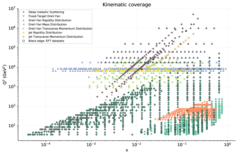
The dataset chosen for this study comprises data points, spanning a broad range of processes including neutral and charged current DIS data (the vast majority of which is composed of the HERA combined dataset) to high mass Drell-Yan measurements from the LHC. The dataset selection is identical to that of Ref. Greljo:2021kvv which is in itself an extension of the strangeness study of Faura:2020oom and NNPDF3.1 Ball:2017nwa . In particular, the neutral current Drell-Yan measurements from ATLAS at , and TeV ATLAS:2013xny ; ATLAS:2016gic and CMS at , , and TeV CMS:2013zfg ; CMS:2014jea ; CMS:2018mdl are LHC measurements that are used to constrain, not only the PDF, but are also sufficiently sensitive to the BSM scenario considered in this work to also constrain the SMEFT operators. The kinematic coverage of the data points used in this study are shown in Fig. 4.1. The points are shown in space with the data points that are modified by the EFT operators highlighted with a border, such points thus also constrain the Wilson coefficients as well as the PDFs. We note that, although DIS theory predictions are modified by the operators we consider in the two benchmark scenarios, the change in the HERA DIS cross sections upon the variation of the Wilson coefficients upon consideration is minimal, as is explicitly assessed in Ref. Greljo:2021kvv .
4.3 Results for Benchmark Scenario I
We first present the results obtained within the first Benchmark Scenario outlined in Sect. 4.1, in which the linear effects are dominant as compared to the quadratic effect and, as a result, SMEFT-modified theoretical predictions are defined as in Eq. (3.2). We start by employing SIMUnet to individually constrain the and operators with the ATLAS and CMS neutral-current (NC) high mass DY data from Run I and Run II. In the next subsection we will be able to constrain them simultaneously thanks to the inclusion of charged-current (CC) HL-LHC projections.
All details about the fit quality, once PDFs are allowed to vary alongside the or the parameters are given in App. B. We observe that the added degrees of freedom result in a slightly better fit quality when compared to the NNPDF4.0-like SM baseline fit based on the reduced dataset described in Sect. 4.2 and on SM theoretical predictions. In particular the high-mass DY datasets that are sensitive to SMEFT corrections display a more significant improvement in fit quality, largely driven by the CMS measurements at TeV, owing to the large weight carried by this dataset, which forms just under half the entire high-mass DY data points hereby considered.
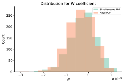
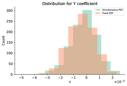
In Figs. 4.2 we show the distribution of the optimal values of and determined for each of the 1000 replicas of the Monte Carlo representation of the experimental data that we obtain during gradient descent in the simultaneous fit of either or and the PDFs. The best-fit values are normally distributed in keeping with the Monte-Carlo pseudodata replica generation that the neural network replicas are fit to. We compare the distribution (in green) with the one that we obtain by keeping the PDFs fixed to the SM baseline (in orange), the latter obtained by using the methodology outlined in Sect. 3.4. Both distributions are centred around zero, illustrating that the high-mass DY datasets are compatible with the SM-only hypothesis, but admit non-zero values, with being less constrained by the data than . The distribution of best fits obtained in a simultaneous fit looks similar to the distribution of best fits obtained by keeping the PDFs fixed to the SM baseline.
| SM PDFs | SMEFT PDFs | best-fit shift | broadening | |
|---|---|---|---|---|
| (68% CL) | +2.6% | |||
| (95% CL) | +3.2% | |||
| (68% CL) | +3.1% | |||
| (95% CL) | +3.1% |
For a more quantitative comparison, in Table 4.1 we compare the bounds for the individual and fits obtained in the simultaneous fits to those obtained by keeping the PDFs fixed to the SM baseline. We indicate the shift and the broadening of the bounds that are obtained once the Wilson coefficients are fitted alongside PDFs, by defining them as
| (4.3) |
| (4.4) |
where is the size of either the 68% C.L. or the 95% C.L., depending on the bounds we consider. The same definitions apply for the parameter. As in Greljo:2021kvv , the effect of fitting the Wilson coefficients simultaneously with the effects that non-zero coefficients have on PDFs changes the interpretation of high-mass DY constraints in a moderate way, with the bounds of the simultaneous fit being within the uncertainty of the current analysis and only slightly looser (by a factor around 3%) than those obtained by keeping the PDFs fixed.
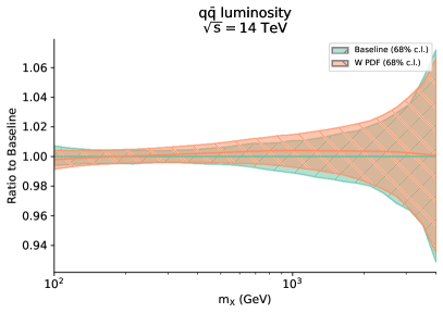
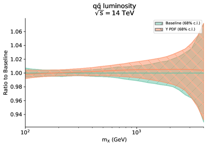
In Figs. 4.3 we show the quark-antiquark channel luminosity plots defined in Eq. (2.9) with the error bands showing C. L., normalised to the baseline SM PDFs. We notice that, while in the previous analysis of Ref. Greljo:2021kvv , we could only produce sets of PDFs obtained at fixed values of and (corresponding to the Benchmark Points that were taken under consideration), here we do really produce a set of PDFs obtained out of a simultaneous fit alongside the Wilson coefficients. We see the luminosity modification due to the simultaneous fit remains moderate, with a slightly larger deviation found at higher values of the produced lepton invariant mass, where the PDFs exhibit slightly larger uncertainties. This is indeed a result consistent with the indications given in Ref. Greljo:2021kvv . Indeed, the dominant luminosity channel for NC DY is and with the valence quark distribution being strongly constrained by DIS and the SMEFT modification being small relative to the experimental uncertainties of the highest invariant mass bins probed by current experimental data. Again, this finding shows that the interplay between EFT effects and PDFs remains moderate when one performs a truly simultaneous determination of both.
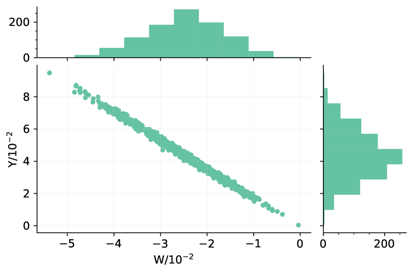
It is interesting to observe that, if we try to fit and at the same time using only the current NC DY data, we identify both the flat direction and the strong anti-correlation between and , which are known to exist in this case Farina:2016rws . Results are shown in Fig. 4.4. Both the flat direction and the anti-correlation can be retrieved within the framework of the SIMUnet methodology, without the user having to be aware of the existence or particular nature of any flat directions which may exist. Indeed, the optimizer cannot preferentially differentiate one point from another within this landscape valley and so the points are distributed tightly along the flat direction. The preference for the upper left quadrant in the - plane is consistent with the findings of Ref. Farina:2016rws with the failure to capture the origin possibly due to the lack of inclusion of terms in the partonic cross section which is known to ease such tensions when only terms are present, as it was pointed out in Ref. Boughezal:2021tih , where the effect of dim-8 operator is carefully assessed.
4.4 Inclusion of the HL-LHC projections
The flat direction illustrated in Fig. 4.4 can be eliminated with the inclusion of Charged Current (CC) DY data Greljo:2021kvv . No unfolded measurements of the high-mass transverse mass distribution have been yet released at 13 TeV, thus we will base our analysis on the High Luminosity LHC (HL-LHC) high-mass Drell-Yan projections that we produced in Ref. Greljo:2021kvv , inspired by the HL-LHC projections studied in Ref. AbdulKhalek:2018rok . The invariant mass distribution projections are generated at TeV, assuming an integrated luminosity of ( collected by ATLAS and by CMS). Both in the case of NC and CC Drell-Yan cross sections, the pseudodata were generated using the MadGraph5_aMCatNLO NLO Monte Carlo event generator Frederix:2018nkq with additional -factors to include the NNLO QCD and NLO EW corrections. The pseudodata consist of four datasets (associated with NC/CC distributions with muons/electrons in the final state), each comprising 16 bins in the invariant mass distribution or transverse mass distributions with both and greater than 500 GeV , with the highest energy bins reaching TeV ( TeV) for NC (CC) data. The rationale behind the choice of number of bins and of the width of each bin was outlined in Ref. Greljo:2021kvv , and stemmed from the requirement that the expected number of events per bin was big enough to ensure the applicability of Gaussian statistics. The choice of binning for the ( ) distribution at the HL-LHC is displayed in Fig. 5.1 of Ref. Greljo:2021kvv .
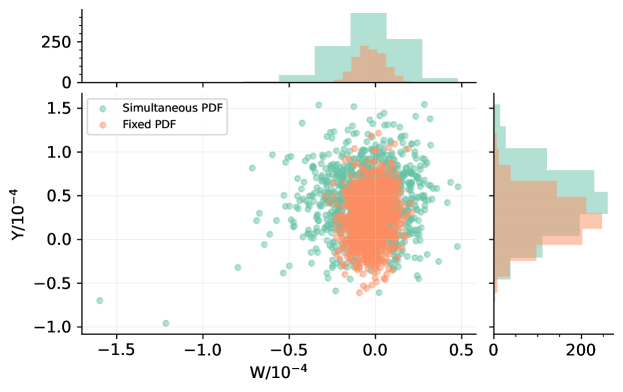
We performed a simultaneous fit of the PDFs and the two parameters by adding two trainable edges in the combination layer displayed in Fig. 3.2, and appending the aforementioned HL-LHC projected data to the data discussed in Sect. 4.2. The best fit values of obtained for each of the 1000 replicas of the Monte Carlo ensemble are plotted in Fig. 4.5. We see that not only is the flat direction of Fig. 4.4 broken, but the HL-LHC projections heavily favour vanishing Wilson coefficients. Indeed, the origin is now covered in both the and axes and much more heavily constrained, enjoying roughly two orders of magnitude tighter constraints in both directions. We notice a slightly favorable pull towards the upper-left quadrant in the - plane, that the ATLAS and CMS datasets seem to prefer. Comparing the best-fit distribution that we get in a simultaneous fit (displayed in green) to the one we get in a fit in which PDFs are kept fixed to the SM baseline (displayed in orange) we can see that the bounds are visibly tighter once PDFs are kept fixed to the SM baseline and are not allowed to consistently vary alongside the Wilson coefficients.
| SM PDFs | SMEFT PDFs | best-fit shift | broadening | |
|---|---|---|---|---|
| (68% CL) | +144% | |||
| (95% CL) | +126% | |||
| (68% CL) | +32% | |||
| (95% CL) | +31% |
In Table 4.2 we compare the bounds for the individual and fits obtained in the simultaneous fits to those obtained by keeping the PDFs fixed to the SM baseline. We indicate the shift and the broadening of the bounds according to the definitions given in Eqs. (4.3)-(4.4). Consistently to what was found in our previous study of Ref. Greljo:2021kvv we observe that including high-mass data at the LHC both in a fit of PDFs and in a fit of SMEFT coefficients and neglecting the interplay between them could result in a significant underestimate of the uncertainties associated to the SMEFT parameters. Indeed, the marginalised bounds on the () parameter increase by about 150% (30%) once a simultaneous fit of the PDFs and the parameters is performed. The broadening is smaller than observed in Ref. Greljo:2021kvv but it is still extremely significant. A detailed comparison is given in Sect. 4.6.
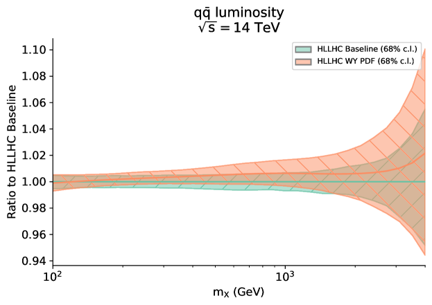
As far ar the quark-antiquark luminosity is concerned, we can see in Fig. 4.6 that once the PDFs are fitted simultaneously with the parameters two things happen. First of all the central values of the luminosity shift upwards for large values of the invariant mass ( 1 TeV) towards the edge of the 68% C.L. error band. Second the error band significantly increases. The shift in the central value is compatible to what we observed before, namely that the luminosity plots, once PDFs are fitted at some representative values of the and parameters, do change significantly, well outside the error band of the SM PDFs, while the PDF uncertainties themselves are unchanged. However, in this case the PDF uncertainty does increase because here we are actually performing a simultaneous fit and, as a result, the PDF error band increases proportionally to the width of the range of and that the data allow. This is a very interesting result and shows that PDF error bands at large- inherently have an extra source of theory uncertainty related with possible BSM effects that the data do not exclude.
4.5 Results for Benchmark Scenario II
In this section we employ the left-handed muon-philic operator to showcase our methodology’s ability to constrain Wilson coefficients whilst accounting for the effect of quadratic dim-6 effects using the approach discussed in Sect. 3.3. The fact that this second Benchmark SMEFT scenario is effectively unconstrained Greljo:2021kvv at the linear level serves to act as the ideal setting to assess the ability to fit EFT operators whilst simultaneously accounting for their quadratic contributions, as in Eq. (3.3). Furthermore, since the operator affects only muon final state observables, while electron final states are described by the SM, the combination layer uses only those datasets that have a muon in the final state to constrain . In particular, the CMS high-mass measurements at 13 TeV, which up until now have been for the combined decay channel, is now separated into the electron and muon channels. As a result of splitting this particular dataset into separate channels, we have accordingly generated a new baseline PDF used in the comparisons.
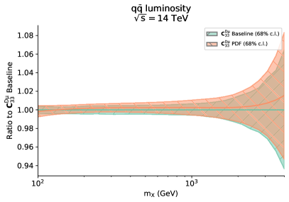
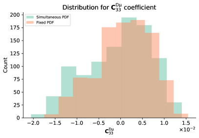
The best-fit values of across the 1000 replicas in the fit are shown on the right-hand panel of Fig. 4.7. We compare the distribution obtained out of a simultaneous fit (in green) with the one obtained once PDFs are kept fixed to the SM baseline (in orange). We see that the distribution of best fit values is centred at the origin, although it is skewed towards . The shape of the distribution is what we expect once quadratic terms are allowed in the fit of the Wilson coefficients by keeping PDF fixed Ethier:2021bye , and it is interesting to see this feature not only holds but it is actually enhanced once the Wilson coefficient is fitted alongside PDFs (green histogram).
| SM PDFs | SMEFT PDFs | best-fit shift | broadening | |
|---|---|---|---|---|
| (68% CL) | +18% | |||
| (95% CL) | +17% |
For a quantitative comparison of the bounds obtained in the simultaneous fit to those obtained in a Wilson coefficient-only fit, in Table 4.3 we show the bounds that we obtain in the two cases. The interplay between PDFs and SMEFT coefficients is quite moderate in this particular scenario. In contrast with the marked effects in Benchmark Scenario I, in Benchmark Scenario II the obtained bounds on this Wilson coefficient would loosen by around 20%. The origin of this rather different behaviour can be traced back to the fact that in this scenario the electron channel data do not receive EFT corrections, and hence all the information that they provide makes it possible to exclusively constrain the PDFs. The muon channel distributions then determine the allowed range for the , restricted by the well-constrained large- quarks and antiquark PDFs from the electron data. This claim is backed by the luminosity comparison, displayed on the left-hand panel of Fig. 4.7: the shift and the increase in the PDF uncertainty of the luminosity are visible, but less enhanced than in the first Benchmark Scenario.
4.6 Results overview
To conclude this section, we present an overview of our results. We have seen in Sect. 4.3 that the current high-mass Drell-Yan data from LHC Run I and Run II do not allow to simultaneously fit and in Benchmark Scenario I and loosely constrain in Benchmark Scenario II. This is mostly due to the lack of unfolded CC Drell-Yan data, which would remove the flat direction that our algorithm is able to detect (see Fig. 4.4). Moreover, our analysis confirms what was outlined in Ref. Greljo:2021kvv , namely that the interplay between the individual fits of and and the fit of the large- quark distributions is mild at the level of current DY data. However, once the high-statistics data projections from the HL-LHC are included, the flat direction disappears and one is able to obtain strong constraints both on the plane Farina:2016rws ; Greljo:2021kvv and on the individual coefficient Greljo:2017vvb ; Greljo:2021kvv . From the point of view of showcasing our methodology, the two scenarios are interesting, as in the Benchmark Scenario I, once the HL-LHC projections are included, we can simultaneously fit both and alongside the PDFs, including only the linear SMEFT corrections while in the Benchmark Scenario II we can fit individually alongside the PDFs, including both the linear and the quadratic SMEFT corrections. In the first scenario, we observe that there is a strong interplay between SMEFT and PDF fits, as the bounds for the SMEFT coefficients significantly broaden once PDFs are allowed to vary alongside and (see Fig. 4.5) and the PDFs themselves display a sizeable shift (see Fig. 4.6). The interplay is more moderate in the second scenario, given that BSM effects only affect the data with muons in the final states, while the data with electrons in the final states constrain the large- quark distributions.
In this section, we focus on the results obtained including the HL-LHC projections. We first explore the correlation patterns between the PDFs and the SMEFT coefficients in both Benchmark Scenarios. These correlation coefficients can be evaluated as in Ref. Carrazza:2019sec . For example in the case of the gluon and the Wilson coefficient, the correlation coefficient is defined as follows
| (4.5) |
where is the best-fit of the coefficient for each replica in the simultaneous fit, in which PDFs are allowed to vary alongside and . In Eq. (4.5), averages are computed over the replicas. This correlation coefficient provides a measure of how the variations in the PDFs translate into modifications of the best fit value of the Wilson coefficients.
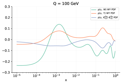
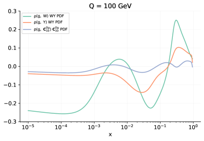
In Fig. 4.8 we show these correlation coefficients between the up valence quark and the gluon PDFs at GeV. Each of the curves corresponds to one of Wilson coefficients considered in the HL-LHC analysis, the and being fitted simultaneously alongside the PDFs (hence the “WY PDF” label) and the being fitted individually alongside the PDFs (hence the “ PDF” label) . Although correlations are moderate, it is interesting to observe that the correlation/anticorrelation between and the PDFs is much stronger than the correlation with the other Wilson coefficients. This explains why the broadening of the bounds in the direction are more marked than those in the directions. Moreover the correlation is stronger in the large- region and for the gluon, which implies an anticorrelation with the singlet in the same region, which is where we observe a broadening of PDF uncertainties.
Throughout the paper we found that the results obtained with the SIMUnet methodology are in line with those presented in Ref. Greljo:2021kvv . In Table 4.4 we make this comparison more quantitative, by focussing on the results in which the effects of the interplay between the SMEFT coefficients and the PDFs are more visible, namely the fits obtained by using the NC and CC projections from the HL-LHC. The results are comparable, although the effect of fitting the Wilson coefficients along with the PDFs is more moderate. This is not surprising, as there are two crucial differences in the two analyses. On the one hand the PDF set that we use here in the fixed SM PDF case is different compared to the one we used in the previous analysis, being based on the same dataset as before but on the NNPDF4.0 methodology rather than the NNPDF3.1 methodology. Secondly, because the previous methodology was based on the use of Benchmark Points in the Wilson coefficients parameter space, we determined the bounds on the parameters by using the partial including only the data affected by the SMEFT corrections, rather than the global . This approximation was forced because the statistical fluctuations of the global were found to be significantly larger than those of the partial and could only be tamed by running a very large batch of replicas for each Benchmark Point and by increasing the density of Benchmark Points in the region that is explored. This approximation is no longer necessary within SIMUnet, because we no longer rely on the interpolation over Benchmark Points, rather we perform a truly simultaneous fit of the PDFs and the Wilson coefficients based on the global . Additionally, the minimizer used in this study employs a momentum driven stochastic gradient descent based algorithm (Nesterov-accelerated adaptive moment estimation kingma2017adam ; Nesterov1983AMF available from the Keras library), while in Ref. Greljo:2021kvv we employed a more traditional genetic algorithm approach using legacy in-house implementations. As such, one in general expects to achieve an improved fit quality with our methodology. Finally, the bounds quoted in our study are defined using Monte Carlo based statistical estimators, whereas in the latter approach, the geometry of the profile is used to define bounds on the Wilson coefficients. Notwithstanding, we observe that the results and the trends are consistent with each other, although the use of the partial over-emphasises the broadening of the bounds.
| SM PDFs | SMEFT PDFs | best-fit shift | broadening | |
|---|---|---|---|---|
| (this work) | +126% | |||
| Greljo:2021kvv | +620% | |||
| (this work) | +31% | |||
| Greljo:2021kvv | +110% | |||
| (this work) | +17% | |||
| Greljo:2021kvv | +18% |
Results in the HL-LHC scenario are displayed in Fig. 4.9.
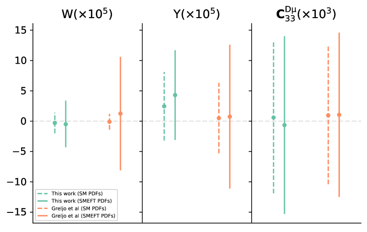
Shown are the results obtained including the current high-mass Drell-Yan data and the projected HL-LHC NC and CC Drell-Yan pseudo-data. In Scenario I, and are fitted simultaneously by keeping only the linear term in the SMEFT expansion, while in Scenario II the coefficients is fitted individually inclusing the quadratic terms in the SMEFT expansion. The results from both studies are compatible, although the bounds obtained from our study are slightly more conservative with differences being explained by the differences between the methodologies employed that are outlined at in this section.
5 Methodology validation and closure testing
In this section, we assess the robustness of our approach through the closure testing framework defined in Refs. Hartland:2019bjb ; DelDebbio:2021whr . Here we do not address the robustness of the PDF part of the fit, which in a sense comes from the results presented in the NNPDF4.0 paper nnpdf40 and the following dedicated study of Ref. DelDebbio:2021whr , but rather focus on the robustness of the fit of the Wilson coefficients and of the PDFs in a simultaneous fit.
Crucially, the central values of the SMEFT-sensitive datasets are modified by artificially contaminating them with pre-chosen, extreme, values of Wilson coefficients. This will emulate a situation where a dataset will favour a non-vanishing EFT operator. In the first part of this section we show that our methodology is sufficiently flexible to recover these chosen values. In the second part of the section we consider the case where the input datasets are replaced by theory predictions from a known underlying PDF set, rather than experimental central values. We show that even in the case of fixing both the underlying PDF and Wilson coefficients to some a priori values, the methodology is sufficiently robust that it can simultaneously reproduce both.
5.1 Closure test results on the Wilson Coefficients
The PDF side of SIMUnet is of course identical to NNPDF4.0 which has been demonstrated to be able to replicate an underlying law using the closure testing framework nnpdf40 ; DelDebbio:2021whr . In this section we will fix the value of the Wilson coefficients a priori and study how effectively we can retrieve these values using our methodology.
To perform this kind of closure tests, we artificially choose extreme values of the Wilson coefficients considered in Benchmark Scenario I, where the interplay between PDF and SMEFT fits is more marked, in two separate analyses:
- 1.
-
2.
The combined fit of the parameters including the HL-LHC projections. Specifically we set , which is also far outside the 95% C. L. contours displayed in Fig. 4.5.
The way we input these non-zero values of the Wilson coefficients in the underlying law is by multiplying the Monte Carlo pseudodata central values by the SMEFT -factors obtained by setting the Wilson coefficient(s) to the aforementioned values. The fitting methodology proceeds as before. Importantly, the entire tool chain has no knowledge of what the value of the Wilson coefficient it is looking for are set to.
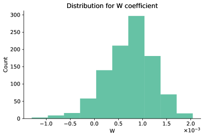
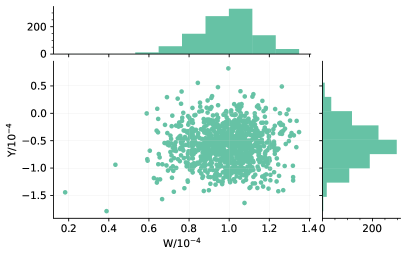
The result of the closure test are displayed in Fig. 5.1. On the left-hand panel we see that the distribution of best fit values of across 1000 replicas, that were previously centred at the origin, now moves considerably towards the a priori value of . Similarly, in the second analysis displayed on the right-hand panel, we see that the presence of HL-LHC data continues to eliminate the flat direction, with the distribution of best fit Wilson coefficients resembling that of Fig. 4.5, but with the best-fits values of the parameters consistently pushed towards the preselecteda priori values of . We see that, despite an extremal choice of the injected values of the Wilson coefficients, the methodology is sufficiently flexible and robust to recover them.
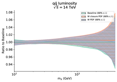
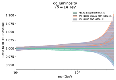
The PDFs generated in the context of the closure tests are displayed in Fig. 5.2. On the left panel, we plot the quark-antiquark luminosity obtained when the experimental central values are modified by inputting (called “W closure PDF”) and compare it to the ones that we obtain in the simultaneously fit of the PDFs and presented in Sect. 4.3 (called “W PDF”), both normalised to the SM baseline. We observe that the PDFs generated with our closure test for are similar to those that we obtain in the simultaneous fit, despite the fact that the training dataset has been heavily modified by the extreme a priori choice of . This is to be expected, since one can view the combination layer as capturing the data’s dependence on the Wilson coefficients, whilst the complementary PDF sector of the network architecture captures the data’s dependence on the underlying PDF, which of course remains unchanged. The combination layer, in effect, subtracts off the EFT dependence, leaving behind the pure SM contribution for the PDF sector to parameterise. This is even more evident in the fit obtained in the presence of the HL-LHC projections, by setting displayed on the right-hand panel of the figure. There we can observe that the central value of the “WY HLLHC closure PDF” luminosity is pushed slightly upwards and the uncertainty is rather smaller once the closure test is performed as compared to the simultaneous fit “WY HLLHC PDF”. This is once again to be expected, given that the range of Wilson Coefficients allowed in the simultaneous fit is larger as compared to the range that we obtain from a simultaneous fit.
5.2 Closure test results on the simultaneous fit
The natural extension of the closure test described in the previous subsection is to assess the degree to which SIMUnet is able to replicate, not only fixed Wilson coefficients, but also a known underlying PDF. For this scenario we employ the NNPDF level 2 NNPDF:2014otw closure test strategy. In the context of a simultaneous fitting methodology this amounts to generating Standard Model predictions using a known PDF set (referred to henceforth as the underlying law) and mapping these to SMEFT observables by multiplying the SM theory predictions with SMEFT K-factors scaled by a previously determined choice of Wilson coefficients. These SMEFT observables, generated by the underlying law, replace the usual MC pseudodata replicas, and are used to train the neural network in the usual way.
Through this approach we are able to assess the degree to which the parameterisation is able to capture not only an underlying choice of Wilson coefficients, but ensures it is sufficiently flexible to adequately replicate a known PDF. For such a closure test, we use the HL-LHC baseline used in this study as the underlying law with the SMEFT scenario being again the simultaneous determination, with the input data being adjusted to have encoded within it.
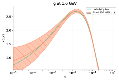
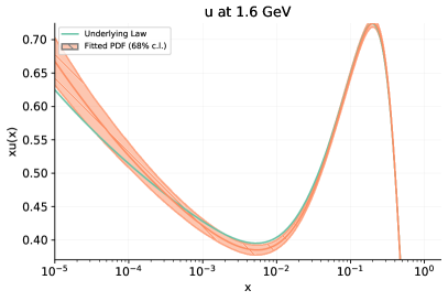
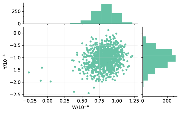
The PDFs generated in this way are shown in Fig. 5.3 for representative choices of parton flavour: we display both the resulting PDFs as well as the underlying law. We see that, despite modifying the training data with an extreme choice of SMEFT benchmark, the methodology is sufficiently robust so as to be able to recover the true PDF set with good precision. Indeed, the distribution of best fit values plotted in Fig. 5.4 shows that not only did the methodology retrieve the underlying law, but also managed to recover the chosen SMEFT scenario: being able to correctly determine the condition. Such behaviour is reminiscent of the above closure test whereby the combination layer is able to parameterise the BSM dynamics while the preceding layers of the model are left to parameterise the PDFs. This conclusion thus illustrates how our methodology is able to correctly disentangle the interplay between PDFs and BSM dynamics.
6 Conclusions and outlook
In this work we have presented a novel methodology, dubbed SIMUnet, which employs the latest in deep learning techniques, to achieve a first truly simultaneous fit of PDFs alongside any physical parameter that determines theoretical predictions at the LHC. As a showcase we fit the Wilson coefficients in the SMEFT and the PDFs in two motivated Benchmark Scenarios.
In particular we employ our methodology to constrain each of and individually using Run I and Run II ATLAS and CMS neutral current (NC) high mass DY data and show that the interplay between SMEFT effects and the fit of large- PDFs remain moderate. Interestingly we show how a scenario like this, displaying a flat direction once and are fitted simultaneously, are uncovered naturally by our approach, without the need for any user intervention or prior knowledge, and how the framework comes to learn that the flat direction is lifted by the inclusion of such data that eliminates this redundancy. Indeed, once the HL-LHC projections are added to the fit, such projections including charged current (CC) DY data, the flat direction is broken and much tighter bounds are obtained.
Most importantly, we confirm the results already shown in our previous analysis of Ref. Greljo:2021kvv , namely that the inclusion of high-mass DY data both in a fit of PDFs and in a fit of SMEFT coefficients by neglecting the interplay between them, could result both in a significant underestimate of the uncertainties associated to the SMEFT parameters (by a factor of 2 in the case of the coefficient) and of the large- PDF uncertainties, that increase by about 70% in the high-mass luminosity regions once the SMEFT affects are accounted for.
We also showcase the ability of our framework to fit SMEFT parameters while including the quadratic effect of SMEFT-SMEFT diagrams. Such a scenario is known Greljo:2021kvv to be essentially unconstrained at linear EFT level and we illustrate how our methodology replicates bounds for presented in previous analyses.
We additionally stress test the methodology by providing it artificially contaminated data possessing data shifted by an a priori choice of Wilson coefficients. We show that our methodology is sufficiently flexible to recover these chosen values. Moreover, we consider the case where the input datasets are replaced by theory predictions from a known underlying PDF set, rather than experimental central values. We show that even in the case of fixing both the underlying PDF and Wilson coefficients to known values, the methodology is sufficiently robust that it can simultaneously reproduce both.
The new methodology that we present here provides a crucial step towards the interpretation of indirect searches under a unified framework. We can assess the impact of new datasets not only on the PDFs, but now on the couplings of an EFT expansion, or on any other physical parameter.
The next steps of our work will include more SMEFT parameters to the combination layer, which is conceptually straightforward. We can add the effects of dim-8 operators or consider the effect of quadratic dim-6 operator effects. Both these scenarios fit very naturally within our approach. Furthermore, one could assess the impact of other high energy datasets from the LHC, exploiting different processes to better constrain other subsets of the Warsaw basis. Finally, an interesting prospect would be to explore simultaneously fitting precision SM parameters, such as the strong coupling or electroweak parameters. Indeed, our framework extends naturally, not only to BSM studies, but to any parameter which may modify the SM prediction through the use of K-factors or other kind of interpolation.
Acknowledgments
We thank Richard Ball, Luigi Del Debbio, Juan Cruz-Martinez, Ben Day, Stefano Forte, James Moore, Juan Rojo, and Zahari Kassabov for particularly useful discussion. We thank the NNPDF collaboration for the public release of the code. We thank the PBSP collaboration for providing the relevant SMEFT -factors for the various datasets studied in this work. M. U. is supported by the European Research Council under the European Union’s Horizon 2020 research and innovation Programme (grant agreement n.950246). M. U. and S. I. are supported by the Royal Society grant RGF/EA/180148. The work of M. U. is also funded by the Royal Society grant DH150088. M. U. and S. I. are partially supported by STFC consolidated grant ST/T000694/1.
Appendix A FK table dependence on the strong coupling
In this appendix we consider the case whereby we wish to isolate the FK table dependence on the strong coupling constant at the -pole, such that, following our notation in Sect. 2, we have . We take the PDG value for the strong coupling evaluated at the -boson mass Zyla:2020zbs to be the point about which we perform the Taylor expansion. The partonic cross sections are given as a power expansion in using perturbation theory, which allows us to write the exact expression
| (A.1) |
where we have simply centred the order by order sum around . For illustrative purposes, we restrict ourselves to the case where the process depends solely on the non-singlet quark distribution. The evolution kernel in Mellin space to leading order in the anomalous dimension (the Mellin transform of the splitting function) , is then given by Ball:2008by :
| (A.2) |
If we consider the leading-log evolution of via renormalisation group equation from to or and set , we get
| (A.3) |
where . Expanding the evolution kernel according to Eq. (2.6), taking , it is easy to see that we get
| (A.4) |
where
| (A.5) | |||
| (A.6) |
Finally, once Eq. (A.4) is combined with Eq. (A.1) we obtain the order by order expansion for the FK tables:
| (A.7) | ||||
| (A.8) |
which can, in principle, be computed and stored permanently in the usual way. In this way we can capture the FK table dependence on the strong coupling parameter in the neighborhood of some prior choice .
So far, we have limited ourselves to the leading order evolution of the PDFs and the strong coupling constant, however a similar expression can be straghtforwardly obtained at next-to-leading (NLO) and next-to-next-to-leading order (NNLO). The only caveat is that, from NLO onwards terms of the form arise which spoil the validity of the Taylor expansion. The term can in principle be made arbitrarily large thus exiting the unit disc which is the region of analyticity of . This problem can be circumvented, however, by noting:
| (A.9) |
where the rightmost term can now be Taylor expanded since can be made arbitrarily small so as to suppress the large logarithm. Indeed, note that in the worst case:
| (A.10) | |||
| (A.11) |
which can be implemented within the optimizer to restrict it from venturing to values greater than .
A viable alternative to the Taylor expansion approach defined in Sect. 2 and detailed here for the simultaneous extraction of and the PDFs is to compute various FK tables using preset values of the strong coupling and then perform an element-wise interpolation between these tensors. In this way one can avoid having to implement the Taylor series expansion, while still accurately replicating the linear behaviour of the FK table. Such a task is reserved for future work prep:as .
Finally if one was to include electroweak corrections to the DGLAP evolution equation, as is for example done in APFEL Bertone:2013vaa , then electroweak parameters will in general also be present in the combined QCD and QED evolution operator. For such a scenario, the prescription outlined in this appendix must then be followed. However, the corrections to the pure QCD splitting functions introduced by electroweak considerations have no dependence on the CKM matrix elements, the weak mixing angle, , or gauge boson masses, amongst others. Such quantities manifest solely in the partonic cross section and in general yield a prescription much simpler than that outlined here.
Appendix B Fit quality
For each MC replica there is the pair which are the best fit PDFs and Wilson coefficients respectively. Together they can be used to generate the corresponding theory predictions for each dataset, noting that any datasets which were not modified by the SMEFT operators will effectively have . We thus have an ensemble of vectors of theory predictions, , with the central theory prediction being given by the average across replicas:
| (B.1) |
The central per data point is then computed in the usual way
| (B.2) |
with being the vector of experimental central values and the covariance matrix encapsulating the experimental uncertainties and the correlations therein. These values are tabulated in Tab. LABEL:tab:_chi2 for each of the various SMEFT scenarios considered in this work. We also tabulate the for various groupings of these datasets, such as DIS only, including or excluding the high-mass DY measurements etc. For these particular entries various correlated systematics may exist between datasets, such as the uncertainty in beam luminosity, which introduces off-diagonal entries in the covariance matrix; as such the grouped is not necessarily equal to the weighted average of the individual values constituting the grouping. This effect is particularly marked for the HL-LHC entries.
| Dataset | ||
|---|---|---|
| SM |
Appendix C Stability on replica number
When performing purely PDF fits to experimental data, it is often the case one will have to compute Monte Carlo PDF replicas in order to achieve a percent level, faithful, uncertainty estimation Ball:2010de . As this study acts as a proof-of-concept for our methodology, we perform high statistic fits composed of MC replicas. However, with each replica requiring approximately 3 hours of compute time, one necessarily requires access to a cluster of nodes in order to asynchronously compute the roughly hours of total wall clock time that is needed for each fit. It is possible, however, to reduce this time by an order of magnitude by instead computing MC replicas per fit, and in this appendix we show that doing so poses little risk in underestimating the statistics when compared to a high replica fit.
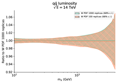
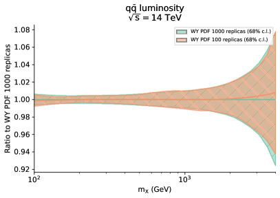
From each of our high replica fits we randomly sample, without replacement, a set of replicas thereby effectively emulating the scenario whereby the user would have performed a low statistics fit. In Fig. B we plot the luminosity for the various SMEFT scenarios considered in this work. We plot the low replica luminosity normalized to the analogous high replica set. We see that the luminosities remain virtually identical, with no discernible difference at the ensemble level. Such behaviour is inherited directly from NNPDF4.0 where a typical fit will typically only possess MC replicas after the post-fit selection has filtered poorly performing replicas.
In Fig. C.2 we present the distributions of best-fit and values using both the high replica and reduced sets. We see that the distribution of best fit Wilson coefficients are accurately reproduced by the low statistics set: implying that, had we stopped the fitting process with 100 MC replicas, the additional 900 replicas would have changed the ensemble statistics such as the mean, standard deviation, or bounds very little. This is a typical pattern in the Monte Carlo approach to PDF fitting, whereby one quickly reaches saturation after MC replicas and further replicas only serve to accurately reproduce the experimental correlations.
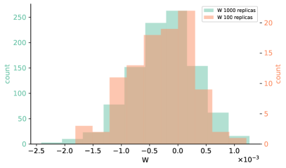
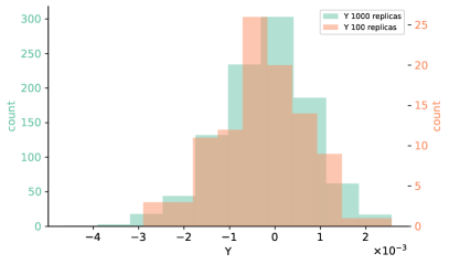
References
- (1) D. Britzger, The Linear Template Fit, arXiv:2112.01548.
- (2) R. D. Ball et al., The Path to Proton Structure at One-Percent Accuracy, arXiv:2109.02653.
- (3) S. Bailey, T. Cridge, L. A. Harland-Lang, A. D. Martin, and R. S. Thorne, Parton distributions from LHC, HERA, Tevatron and fixed target data: MSHT20 PDFs, Eur. Phys. J. C 81 (2021), no. 4 341, [arXiv:2012.04684].
- (4) T.-J. Hou et al., New CTEQ global analysis of quantum chromodynamics with high-precision data from the LHC, Phys. Rev. D 103 (2021), no. 1 014013, [arXiv:1912.10053].
- (5) S. Alekhin, J. Blümlein, S. Moch, and R. Placakyte, Parton distribution functions, , and heavy-quark masses for LHC Run II, Phys. Rev. D 96 (2017), no. 1 014011, [arXiv:1701.05838].
- (6) Particle Data Group Collaboration, P. Zyla et al., Review of Particle Physics, PTEP 2020 (2020), no. 8 083C01.
- (7) SMEFiT Collaboration, J. J. Ethier, G. Magni, F. Maltoni, L. Mantani, E. R. Nocera, J. Rojo, E. Slade, E. Vryonidou, and C. Zhang, Combined SMEFT interpretation of Higgs, diboson, and top quark data from the LHC, JHEP 11 (2021) 089, [arXiv:2105.00006].
- (8) J. Ellis, M. Madigan, K. Mimasu, V. Sanz, and T. You, Top, Higgs, Diboson and Electroweak Fit to the Standard Model Effective Field Theory, JHEP 04 (2021) 279, [arXiv:2012.02779].
- (9) S. Forte and Z. Kassabov, Why cannot be determined from hadronic processes without simultaneously determining the parton distributions, Eur. Phys. J. C 80 (2020), no. 3 182, [arXiv:2001.04986].
- (10) S. Alekhin, S. Moch, and S. Thier, Determination of the top-quark mass from hadro-production of single top-quarks, Phys. Lett. B 763 (2016) 341–346, [arXiv:1608.05212].
- (11) E. Bagnaschi and A. Vicini, Parton Density Uncertainties and the Determination of Electroweak Parameters at Hadron Colliders, Phys. Rev. Lett. 126 (2021), no. 4 041801, [arXiv:1910.04726].
- (12) H1 Collaboration, V. Andreev et al., Determination of electroweak parameters in polarised deep-inelastic scattering at HERA, Eur. Phys. J. C 78 (2018), no. 9 777, [arXiv:1806.01176].
- (13) J. J. Ethier and E. R. Nocera, Parton Distributions in Nucleons and Nuclei, Ann. Rev. Nucl. Part. Sci. 70 (2020) 43–76, [arXiv:2001.07722].
- (14) R. A. Khalek, J. J. Ethier, E. R. Nocera, and J. Rojo, Self-consistent determination of proton and nuclear PDFs at the Electron Ion Collider, Phys. Rev. D 103 (2021), no. 9 096005, [arXiv:2102.00018].
- (15) NNPDF Collaboration, V. Bertone, N. P. Hartland, E. R. Nocera, J. Rojo, and L. Rottoli, Charged hadron fragmentation functions from collider data, Eur. Phys. J. C 78 (2018), no. 8 651, [arXiv:1807.03310].
- (16) I. Brivio and M. Trott, The Standard Model as an Effective Field Theory, Phys. Rept. 793 (2019) 1–98, [arXiv:1706.08945].
- (17) A. Greljo, S. Iranipour, Z. Kassabov, M. Madigan, J. Moore, J. Rojo, M. Ubiali, and C. Voisey, Parton distributions in the SMEFT from high-energy Drell-Yan tails, JHEP 07 (2021) 122, [arXiv:2104.02723].
- (18) S. Carrazza, C. Degrande, S. Iranipour, J. Rojo, and M. Ubiali, Can New Physics hide inside the proton?, Phys. Rev. Lett. 123 (2019), no. 13 132001, [arXiv:1905.05215].
- (19) ZEUS Collaboration, H. Abramowicz et al., Limits on contact interactions and leptoquarks at HERA, Phys. Rev. D 99 (2019), no. 9 092006, [arXiv:1902.03048].
- (20) CMS Collaboration, A. Tumasyan et al., Measurement and QCD analysis of double-differential inclusive jet cross sections in proton-proton collisions at = 13 TeV, arXiv:2111.10431.
- (21) NNPDF Collaboration, R. D. Ball et al., An open-source machine learning framework for global analyses of parton distributions, Eur. Phys. J. C 81 (2021), no. 10 958, [arXiv:2109.02671].
- (22) R. D. Ball, L. Del Debbio, S. Forte, A. Guffanti, J. I. Latorre, J. Rojo, and M. Ubiali, A first unbiased global NLO determination of parton distributions and their uncertainties, Nucl. Phys. B 838 (2010) 136–206, [arXiv:1002.4407].
- (23) R. D. Ball et al., Parton distributions with LHC data, Nucl. Phys. B 867 (2013) 244–289, [arXiv:1207.1303].
- (24) V. Bertone, S. Carrazza, and N. P. Hartland, APFELgrid: a high performance tool for parton density determinations, Comput. Phys. Commun. 212 (2017) 205–209, [arXiv:1605.02070].
- (25) A. G. Baydin, B. A. Pearlmutter, A. A. Radul, and J. M. Siskind, Automatic differentiation in machine learning: a survey, 2018.
- (26) M. González-Alonso, J. Martin Camalich, and K. Mimouni, Renormalization-group evolution of new physics contributions to (semi)leptonic meson decays, Phys. Lett. B 772 (2017) 777–785, [arXiv:1706.00410].
- (27) E. E. Jenkins, A. V. Manohar, and M. Trott, Renormalization Group Evolution of the Standard Model Dimension Six Operators II: Yukawa Dependence, JHEP 01 (2014) 035, [arXiv:1310.4838].
- (28) E. E. Jenkins, A. V. Manohar, and M. Trott, Renormalization Group Evolution of the Standard Model Dimension Six Operators I: Formalism and lambda Dependence, JHEP 10 (2013) 087, [arXiv:1308.2627].
- (29) A. Greljo and D. Marzocca, High- dilepton tails and flavor physics, Eur. Phys. J. C 77 (2017), no. 8 548, [arXiv:1704.09015].
- (30) R. Torre, L. Ricci, and A. Wulzer, On the W&Y interpretation of high-energy Drell-Yan measurements, JHEP 02 (2021) 144, [arXiv:2008.12978].
- (31) S. Carrazza and J. Cruz-Martinez, Towards a new generation of parton densities with deep learning models, Eur. Phys. J. C 79 (2019), no. 8 676, [arXiv:1907.05075].
- (32) NNPDF Collaboration, R. D. Ball et al., Parton distributions from high-precision collider data, Eur. Phys. J. C 77 (2017), no. 10 663, [arXiv:1706.00428].
- (33) M. Abadi, P. Barham, J. Chen, Z. Chen, A. Davis, J. Dean, M. Devin, S. Ghemawat, G. Irving, M. Isard, et al., Tensorflow: A system for large-scale machine learning, in 12th USENIX Symposium on Operating Systems Design and Implementation (OSDI 16), pp. 265–283, 2016.
- (34) J. Bergstra, B. Komer, C. Eliasmith, D. Yamins, and D. D. Cox, Hyperopt: a Python library for model selection and hyperparameter optimization, Computational Science and Discovery 8 (Jan., 2015) 014008.
- (35) NNPDF Collaboration, R. D. Ball, L. Del Debbio, S. Forte, A. Guffanti, J. I. Latorre, J. Rojo, and M. Ubiali, Fitting Parton Distribution Data with Multiplicative Normalization Uncertainties, JHEP 05 (2010) 075, [arXiv:0912.2276].
- (36) G. D’Agostini, On the use of the covariance matrix to fit correlated data, Nucl. Instrum. Meth. A346 (1994) 306–311.
- (37) NNPDF Collaboration, R. Abdul Khalek et al., Parton Distributions with Theory Uncertainties: General Formalism and First Phenomenological Studies, Eur. Phys. J. C 79 (2019), no. 11 931, [arXiv:1906.10698].
- (38) NNPDF Collaboration, R. Abdul Khalek et al., A first determination of parton distributions with theoretical uncertainties, Eur. Phys. J. C (2019) 79:838, [arXiv:1905.04311].
- (39) R. D. Ball, E. R. Nocera, and R. L. Pearson, Deuteron Uncertainties in the Determination of Proton PDFs, Eur. Phys. J. C 81 (2021), no. 1 37, [arXiv:2011.00009].
- (40) C. M. Bishop et al., Neural networks for pattern recognition. Oxford university press, 1995.
- (41) NNPDF Collaboration, L. Del Debbio, S. Forte, J. I. Latorre, A. Piccione, and J. Rojo, Neural network determination of parton distributions: The Nonsinglet case, JHEP 03 (2007) 039, [hep-ph/0701127].
- (42) NNPDF Collaboration, R. D. Ball, L. Del Debbio, S. Forte, A. Guffanti, J. I. Latorre, A. Piccione, J. Rojo, and M. Ubiali, A Determination of parton distributions with faithful uncertainty estimation, Nucl. Phys. B 809 (2009) 1–63, [arXiv:0808.1231]. [Erratum: Nucl.Phys.B 816, 293 (2009)].
- (43) J. Bergstra, D. Yamins, and D. Cox, Making a science of model search: Hyperparameter optimization in hundreds of dimensions for vision architectures, in International conference on machine learning, pp. 115–123, PMLR, 2013.
- (44) R. Boughezal, E. Mereghetti, and F. Petriello, Dilepton production in the SMEFT at , arXiv:2106.05337.
- (45) C. Grojean, E. E. Jenkins, A. V. Manohar, and M. Trott, Renormalization Group Scaling of Higgs Operators and Decay, JHEP 04 (2013) 016, [arXiv:1301.2588].
- (46) J. Baglio, S. Dawson, and S. Homiller, QCD corrections in Standard Model EFT fits to and production, Phys. Rev. D 100 (2019), no. 11 113010, [arXiv:1909.11576].
- (47) C. Degrande, G. Durieux, F. Maltoni, K. Mimasu, E. Vryonidou, and C. Zhang, Automated one-loop computations in the standard model effective field theory, Phys. Rev. D 103 (2021), no. 9 096024, [arXiv:2008.11743].
- (48) S. Dawson and P. P. Giardino, New Physics Through Drell Yan SMEFT Measurements at NLO, arXiv:2105.05852.
- (49) H.-L. Li, Z. Ren, J. Shu, M.-L. Xiao, J.-H. Yu, and Y.-H. Zheng, Complete set of dimension-eight operators in the standard model effective field theory, Phys. Rev. D 104 (2021), no. 1 015026, [arXiv:2005.00008].
- (50) C. W. Murphy, Dimension-8 operators in the Standard Model Eective Field Theory, JHEP 10 (2020) 174, [arXiv:2005.00059].
- (51) J. Davighi, S. Melville, and T. You, Natural Selection Rules: New Positivity Bounds for Massive Spinning Particles, arXiv:2108.06334.
- (52) NNPDF Collaboration, R. D. Ball et al., Parton distributions for the LHC Run II, JHEP 04 (2015) 040, [arXiv:1410.8849].
- (53) M. E. Peskin and T. Takeuchi, Estimation of oblique electroweak corrections, Phys. Rev. D 46 (1992) 381–409.
- (54) G. Altarelli, R. Barbieri, and S. Jadach, Toward a model independent analysis of electroweak data, Nucl. Phys. B 369 (1992) 3–32. [Erratum: Nucl.Phys.B 376, 444 (1992)].
- (55) R. Barbieri, A. Pomarol, R. Rattazzi, and A. Strumia, Electroweak symmetry breaking after LEP-1 and LEP-2, Nucl. Phys. B 703 (2004) 127–146, [hep-ph/0405040].
- (56) M. Farina, G. Panico, D. Pappadopulo, J. T. Ruderman, R. Torre, and A. Wulzer, Energy helps accuracy: electroweak precision tests at hadron colliders, Phys. Lett. B 772 (2017) 210–215, [arXiv:1609.08157].
- (57) G. Panico, L. Ricci, and A. Wulzer, High-energy EFT probes with fully differential Drell-Yan measurements, JHEP 07 (2021) 086, [arXiv:2103.10532].
- (58) LHCb Collaboration, R. Aaij et al., Test of lepton universality using decays, Phys. Rev. Lett. 113 (2014) 151601, [arXiv:1406.6482].
- (59) LHCb Collaboration, R. Aaij et al., Test of lepton universality with decays, JHEP 08 (2017) 055, [arXiv:1705.05802].
- (60) LHCb Collaboration, R. Aaij et al., Search for lepton-universality violation in decays, Phys. Rev. Lett. 122 (2019), no. 19 191801, [arXiv:1903.09252].
- (61) F. Faura, S. Iranipour, E. R. Nocera, J. Rojo, and M. Ubiali, The Strangest Proton?, Eur. Phys. J. C 80 (2020), no. 12 1168, [arXiv:2009.00014].
- (62) ATLAS Collaboration, G. Aad et al., Measurement of the high-mass Drell–Yan differential cross-section in pp collisions at TeV with the ATLAS detector, Phys. Lett. B 725 (2013) 223–242, [arXiv:1305.4192].
- (63) ATLAS Collaboration, G. Aad et al., Measurement of the double-differential high-mass Drell-Yan cross section in pp collisions at TeV with the ATLAS detector, JHEP 08 (2016) 009, [arXiv:1606.01736].
- (64) CMS Collaboration, S. Chatrchyan et al., Measurement of the Differential and Double-Differential Drell-Yan Cross Sections in Proton-Proton Collisions at 7 TeV, JHEP 12 (2013) 030, [arXiv:1310.7291].
- (65) CMS Collaboration, V. Khachatryan et al., Measurements of differential and double-differential Drell-Yan cross sections in proton-proton collisions at 8 TeV, Eur. Phys. J. C 75 (2015), no. 4 147, [arXiv:1412.1115].
- (66) CMS Collaboration, A. M. Sirunyan et al., Measurement of the differential Drell-Yan cross section in proton-proton collisions at = 13 TeV, JHEP 12 (2019) 059, [arXiv:1812.10529].
- (67) R. Abdul Khalek, S. Bailey, J. Gao, L. Harland-Lang, and J. Rojo, Towards Ultimate Parton Distributions at the High-Luminosity LHC, Eur. Phys. J. C 78 (2018), no. 11 962, [arXiv:1810.03639].
- (68) R. Frederix, S. Frixione, V. Hirschi, D. Pagani, H. S. Shao, and M. Zaro, The automation of next-to-leading order electroweak calculations, JHEP 07 (2018) 185, [arXiv:1804.10017]. [Erratum: JHEP 11, 085 (2021)].
- (69) D. P. Kingma and J. Ba, Adam: A method for stochastic optimization, arXiv:1412.6980.
- (70) Y. Nesterov, A method for solving the convex programming problem with convergence rate , Proceedings of the USSR Academy of Sciences 269 (1983) 543–547.
- (71) N. P. Hartland, F. Maltoni, E. R. Nocera, J. Rojo, E. Slade, E. Vryonidou, and C. Zhang, A Monte Carlo global analysis of the Standard Model Effective Field Theory: the top quark sector, JHEP 04 (2019) 100, [arXiv:1901.05965].
- (72) L. Del Debbio, T. Giani, and M. Wilson, Bayesian Approach to Inverse Problems: an Application to NNPDF Closure Testing, arXiv:2111.05787.
- (73) S. Iranipour et al., A simultaneous determination of PDFs and using deep-learning., in preparation.
- (74) V. Bertone, S. Carrazza, and J. Rojo, APFEL: A PDF Evolution Library with QED corrections, Comput. Phys. Commun. 185 (2014) 1647–1668, [arXiv:1310.1394].