Synchronization of Coupled Phase Oscillators
with Stochastic Disturbances and
the Cycle Space of the Graph

Abstract

The synchronization stability of a complex network system of coupled phase oscillators is discussed. In case the network is affected by disturbances, a stochastic linearized system of the coupled phase oscillators may be used to determine the fluctuations of phase differences in the lines between the nodes and to identify the vulnerable lines that may lead to desynchronization. The main result is the derivation of the asymptotic variance matrix of the phase differences which characterizes the severity of the fluctuations. It is found that the cycle space of the graph of the system plays a role in this characterization. With theory of the cycle space, the effect of forming small cycles on the fluctuations are evaluated. It is proven that adding a new line or increasing the coupling strength of a line affect the fluctuations in the lines in any cycle including this line while it does not affect the fluctuations in the other lines. In particular, if the phase differences at the synchronous state are not changed by these actions, then the affected fluctuations reduce.

05C38, 34C15, 34D06, 34D20, 90B15, 93E03.

1 Introduction

Synchronization in a networked system of coupled phase oscillators serves as a paradigm for understanding of the collective behavior of a real complex networked system. A coupled oscillator network is characterized by a population of heterogeneous oscillators and a graph describing the interaction among the oscillators. Examples of such systems arise in nature (e.g., Kuramoto oscillators [17], chimera spatiotemporal patterns [1], cardiac pacemaker cells [11]) and in technological systems (for example, multi-agent systems [19], consensus problems [7], distributed optimization [31], power grids [30, 21]).

In this paper, we focus on systems which need synchronization for proper functioning, such as power grids. If the synchronization is lost, then the systems can no longer function properly. The vast literature shows that significant insights have been obtained on the emergence of a synchronous state (defined to be a steady state of the system) and synchronization coherence. The synchronization is determined by the system parameters, including the natural frequencies at the nodes, the network topology and the coupling strength of lines. With the metrics of the critical coupling strength [7, 8, 10] and the order parameter [26], the effects of these parameters on the synchronization are widely investigated. Based on these investigations, the system parameters may be assigned to optimize the synchrony, which can be attained by deletion or addition of lines, or by changing the coupling strength of the lines in the network. An important problem is to maintain the synchronization when the system is subjected to disturbances. Regarding the ability to maintain the synchronization, the spectrum of the system matrix of the linearized system and the volume of the basin of attraction of a stable synchronous state may be investigated. However, in these investigations, the severity of the disturbances are not considered and the lines at which the synchronization may be lost cannot be effectively identified. The question how disturbances spread through networks of power systems, has attracted wide interest of investigation with a toolbox for simulations and with analytic methods [16, 34, 2, 20]. In control theory, the synchronous state is mentioned as the set point for control, in which control actions are taken to let the state converge to the synchronous state after disturbances. Thus, under continuous disturbances, the phase may fluctuate around the synchronous state. If the fluctuations of the phase differences are larger than the threshold $\pi/2$, a synchronous state may not be attained any longer, and then the synchronization may be lost [13]. This indicates the necessity to study the phase difference in the lines but not the phases at the nodes. One says that a line is vulnerable if the desynchronization occurs at this line easily. Clearly, the lines with large fluctuations in the phase difference are vulnerable. Modelling the disturbances by inputs to the system, the $\mathcal{H}_{2}$ norm of a linear input-output system has been widely used to study the fluctuations of the phase differences [24, 27]. With this $\mathcal{H}_{2}$ norm, the fluctuations may be effectively suppressed by assigning the system parameters, thus improve the robustness of the system. However, because the $\mathcal{H}_{2}$ norm equals to the trace of a matrix [27], which is a global metric characterizing the sum of the fluctuations, the fluctuations of the phase differences in the lines and their correlation can hardly be explicitly characterized.

In this paper, we investigate the dependence of the fluctuations of the phase differences in each line on the system parameters analytically, which can be used to suppress the fluctuations and identify the vulnerable lines, thus improve the ability of the system to maintain the synchronization. We model the disturbance by a set of Brownian motions and reformulate the system as a stochastic linear system. It is well known that for a linear Gaussian stochastic system with a system matrix that is Hurwitz, there exists an invariant probability distribution of the state that is a Gaussian probability distribution characterized by the mean value and the asymptotic variance of the state [18, Theorem 1.53][15, Theorem 6.7]. In the invariant distribution, the asymptotic variance characterizes the severity of the fluctuations in the phase difference in each line of the system. The focus of this paper is on the asymptotic variance of a stochastic linearized network system of coupled phase oscillators, which reveals how the fluctuations in the phase differences depend on the system parameters. With the asymptotic matrix as a metric, a new avenue is open to study the robustness of network systems against the disturbances. The contribution of this paper include explicit formulas of the asymptotic variance matrix and findings from these formulas on the impact of adding new lines and strengthening the coupling of the oscillators. To the best knowledge of the authors, for the first time the cycle space of a graph is related to the robustness of the system by an explicit formula. The method to study the synchronization stability in this paper can be extended to the networks with synchronizations, such as the power systems [32] and the general diffusive network [26].

The paper is structured as follows. Section 2 provides elementary preliminaries on graphs theory and the invariant probability distribution of stochastic process. We formulate problem of the complex network of coupled phase oscillators and present the main results on the asymptotic variance in Section 3. The findings from the asymptotic variance are illustrated in three example networks in Section 4. Section 5 provides the proofs of the results and Section 6 concludes with remarks.

2 Preliminaries

The elementary notation, properties of graphs and the cycle space and the concept of the asymptotic variance of a stochastic Gaussian system are introduced in this section.

2.1 Notations

The set of the integers is denoted by $\mathbb{Z}=\{\ldots,~{}-1,~{}0,~{}1,~{}2,\ldots\}$ and that of the positive integers by $\mathbb{Z}_{+}=\{1,~{}2,~{}\ldots\}$. For any integer $n\in\mathbb{Z}$ denote the set of the first $n$ positive integers by $\mathbb{Z}_{n}=\{1,~{}2,~{}\ldots,~{}n\}$. The set of the real numbers is denote by $\mathbb{R}$. Denote the strictly positive real numbers by $\mathbb{R}_{+}=(0,~{}+\infty)$.

The vector space of $n$-tuples of the real numbers is denoted by $\mathbb{R}^{n}$ for an integer $n\in\mathbb{Z}_{+}$. For the integers $n,~{}m\in\mathbb{Z}_{+}$ the set of $n$ by $m$ matrices with entries of the real numbers, is denoted by $\mathbb{R}^{n\times m}$. Denote the identity matrix of size $n$ by $n$ by $\mathbf{I}_{n}\in\mathbb{R}^{n\times n}$, which may also be denoted by $\mathbf{I}$ if the size is clear from the context.

Denote subsets of matrices according to: for an integer $n\in\mathbb{Z}_{+}$, $\mathbb{R}_{spd}^{n\times n}$ denotes the subset of symmetric positive semi-definite matrices of which an element is denoted by $0\preceq\mathbf{Q}=\mathbf{Q}^{\top}$;

for matrices $\mathbf{A}\in\mathbb{R}^{n\times n}$ and $\mathbf{B}\in\mathbb{R}^{n\times n}$, denote by $\mathbf{A}\preceq\mathbf{B}$ that $\mathbf{B}-\mathbf{A}$ is semi-positive-definite; $\mathbb{R}_{nsng}^{n\times n}$ the subset of nonsingular square matrices; $\mathbb{R}_{ortg}^{n\times n}$ the subset of orthogonal matrices which by definition satisfy $\mathbf{U}~{}\mathbf{U}^{\top}=\mathbf{I}_{n}=\mathbf{U}^{\top}~{}\mathbf{U}$. Call a square matrix $\mathbf{A}\in\mathbb{R}^{n\times n}$ Hurwitz if all eigenvalues have a real part which is strictly negative; in terms of notation, for any eigenvalue $\lambda(\mathbf{A})$ of the matrix $\mathbf{A}$, $\mbox{$\mathrm{Re}$}(\lambda(\mathbf{A}))<0$.

2.2 Graphs and the Cycle Space

Consider an undirected weighted network $\mathcal{G}=(\mathcal{V},\mathcal{E})$ with a set of $n\in\mathbb{Z}_{+}$ nodes denoted by $\mathcal{V}$ and a set of $m\in\mathbb{Z}_{+}$ edges or lines denoted by $\mathcal{E}$ and line weight $w_{ij}=w_{ji}\in\mathbb{R}_{+}$ if the nodes $i$ and $j$ are connected and $w_{ij}=0$ otherwise. Denote by $k=(i,~{}j)\in\mathcal{E}$ the edge connecting the nodes $i$ and $j$ which edge is also denoted by $k$. The Laplacian matrix of the graph is defined as $\mathbf{L}=(l_{{ij}})\in\mathbb{R}^{n\times n}$ with

(3) $$l_{ij}=\left\{\begin{array}[]{ll}-w_{ij},&\mbox{if}~{}i\neq j,\\ -\sum_{k=1,~{}k\neq i}^{n}~{}w_{ik}&\mbox{if}~{}i=j.\end{array}\right.$$

The incidence matrix is defined as $\mathbf{C}=(C_{ik})\in\mathbb{R}^{n\times m}$ with $C_{ik}\in\mathbb{R}$,

(7) $$C_{ik} = \left\{\begin{array}[]{rl}1,&\text{if node $i$ is the beginning of line $e_{k}$},\\ -1,&\text{if node $i$ is the end of line $e_{k}$},\\ 0,&\text{otherwise},\end{array}\right.$$

Here the direction of line $e_{k}$ is arbitrarily specified in order to define the incidence matrix. We further define a diagonal matrix $\mathbf{R}=\text{diag}(R_{k})\in\mathbb{R}^{m\times m}$ with $R_{k}=w_{ij}$ being the weight of line $e_{k}$ with $k=(i,j)\in\mathcal{E}$. Elementary properties of matrices which are needed subsequently are summarized in the next lemma.

Lemma 2.1.

Consider the graph $\mathcal{G}$ with matrices $\mathbf{L},\mathbf{C},\mathbf{R}$.

• The Laplacian matrix $\mathbf{L}$ is symmetric and hence all its eigenvalues are real.

• Following the Gerschgorin’ theorem [22, Theorem 36], all the eigenvalues of $\mathbf{L}$ are non-negative.

• Denote the eigenvalues of $\mathbf{L}$ by $0\leq\mu_{1}\leq\mu_{2}\leq\cdots\leq\mu_{n}$. It holds $\mathbf{L}\mathbf{1}_{n}=\mathbf{0}_{n}$, thus, $\mu_{1}=0$ is an eigenvalue of $\mathbf{L}$ with an eigenvector $\tau\mathbf{1}_{n}$ where $\tau\in\mathbb{R}$.

• The graph $\mathcal{G}$ is connected if and only if the second smallest eigenvalue $\mu_{2}>0$ [22, Theorem 10].

• A relation between the incidence matrix $\mathbf{C}$ and the Laplacian matrix $\mathbf{L}$ is

  (8) $$\mathbf{C}\mathbf{R}\mathbf{C}^{\top}=\mathbf{L}.$$

• It holds $\mathbf{C}^{\top}\mathbf{1}_{n}=\mathbf{0}_{m}$.

• If the graph $\mathcal{G}$ is connected, then $rank(\mathbf{C})=n-1$ [22, Theorem 1].

The concept of the cycle space of the graph plays an important role in the characterization of the asymptotic variance matrix in this paper, which is defined below.

Definition 2.2.

Consider a connected and undirected graph $\mathcal{G}=(\mathcal{V},\mathcal{E})$ with matrix $\mathbf{C}$.

• If $\mathcal{C}$ is a subset of $\mathcal{E}$ such that the subgraph formed by $\mathcal{C}$ is a cycle graph,in which there are at least three nodes, the number of nodes equals to the number of lines and all the nodes are in a path that starts and ends at the same node without repeating any lines, then $\mathcal{C}$ is a cycle in $\mathcal{G}$.

• Let $\mathcal{T}$ be a spanning tree of $\mathcal{G}$, then there are $n-1$ edges in $\mathcal{T}$ and $m-n+1$ edges of $\mathcal{G}$ lie outside of $\mathcal{T}$. For each of these $m-n+1$ edges $e\in\mathcal{E}\backslash\mathcal{E}(\mathcal{T})$, the graph $\mathcal{T}+e$ contains a unique cycle in which the lines forms a fundamental cycle of the graph $\mathcal{G}$.

• The cycle space of graph $\mathcal{G}$ is defined as the kernel of the incidence matrix $\mathbf{C}$,

  $$\mathbf{X}_{cysp} = \ker(\mathbf{C})=\{\mathbf{\xi}\in\mathbb{R}^{m}|~{}\mathbf{C}\mathbf{\xi}=\mathbf{0}_{n}\}\subseteq\mathbb{R}^{m},$$

  $$\dim(\mathbf{X}_{cysp}) = n_{cysp}=m-\mbox{${\mathrm{rank}}$}(\mathbf{C})=m-n+1.$$

The basis vectors of the cycle space can be derived based on the following theorem.

Theorem 2.3.

[3, Theorem 4.5,Theorem 5.2][4, Chapter 4] Consider a connected and undirected graph $\mathcal{G}=(\mathcal{V},\mathcal{E})$ with matrix $\mathbf{C}$.

• For a cycle $\mathcal{C}_{c}$ with set $\mathcal{E}_{c}$ of lines in the graph $\mathcal{G}$, we specify a direction for $\mathcal{C}_{c}$ and define a vector for the cycle,

  $$\mathbf{\xi}_{c} = \begin{bmatrix}\xi_{c,1}&\xi_{c,2}&\cdots&\xi_{c,m}\end{bmatrix}^{\top}\in\mathbb{R}^{m},$$

  $$\xi_{c,k} = \begin{cases}+1,&\text{ if $e_{k}\in\mathcal{E}_{c}$ with direction $=$ the cycle direction },\\ -1,&\text{ if $e_{k}\in\mathcal{E}_{c}$ with direction $\neq$ the cycle direction },\\ 0,&\text{ otherwise,}\end{cases}$$

  Then, it satisfies $\mathbf{C}\mathbf{\xi}_{c}=\mathbf{0}$, thus, $\mathbf{\xi}_{c}$ belongs to the kernel of $\mathbf{C}$.

• A set of basis vectors of the cycle space can be derived by taking the vectors as $\mathbf{\xi}_{c}$ for $c=1,\cdots,m-n+1$ corresponding to the $(m-n+1)$  fundamental cycles

If the direction of the cycle $\mathcal{C}_{c}$ is changed, the vector $-\xi_{c}$ is obtained, which can also be a basis vector of the kernel of the cycle space. Thus, to obtain the basis vectors of the cycle space, the directions of the cycles can be specified arbitrarily, which is independent of the directions of the lines specified for the definition of the incidence matrix.

We take the networks in Fig.1 as examples to illustrate the cycle space of graphs and its basis vectors. The directions of the lines are arbitrarily specified, and the directions of all the cycles are chosen to be clockwise. These directions are set for the calculation of the incidence matrix $\mathbf{C}$ and the basis vectors of the cycle space, which does not mean the networks are directed. The network (a) is a tree network hence $m=n-1$, thus the dimension of the kernel of the incidence matrix is zero and no basis vectors can be formulated. For network (b), the basis vectors of the cycle space are $\mathbf{\xi}_{1}=[0,0,0,0,0,-1,1,-1,0]^{\top}$ and $\mathbf{\xi}_{2}=[0,-1,1,-1,0,0,0,0,1]^{\top}$ corresponding to the cycles $\{e_{2},e_{3},e_{4},e_{9}\}$ and $\{e_{6},e_{7},e_{8}\}$ respectively. For network (c), the basis vectors of the cycle space are $\mathbf{\xi}_{1}=[0,0,0,0,0,-1,1,-1,0]^{\top}$, $\mathbf{\xi}_{2}=[0,-1,1,-1,0,0,0,0,1]^{\top}$ and $\mathbf{\xi}_{3}=[1,0,0,0,0,0,0,0,-1,1]$ corresponding to the cycles $\{e_{2},e_{3},e_{4},e_{9}\}$ and $\{e_{6},e_{7},e_{8}\}$ and $\{e_{1},e_{9},e_{10}\}$ respectively. Note that for the graph with cycles, because the spanning tree may not be unique, the set of the basis vectors of the cycle space may be non-unique. For example, for network (c), the basis vectors of the cycle space can also be $\mathbf{\xi}_{1}=[0,0,0,0,0,-1,1,-1,0]^{\top}$, $\mathbf{\xi}_{2}=[0,-1,1,-1,0,0,0,0,1]^{\top}$ and $\mathbf{\xi}_{3}=[1,-1,1,-1,0,0,0,0,0,1]$ corresponding to the cycles $\{e_{2},e_{3},e_{4},e_{9}\}$ and $\{e_{6},e_{7},e_{8}\}$ and $\{e_{1},e_{2},e_{3},e_{4},e_{10}\}$ respectively.

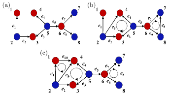
Figure 1: Three networks with 8 nodes.

2.3 The Asymptotic Variance

Consider a time-invariant linear stochastic differential equation with representation,

$$\text{d}\mathbf{x}(t) = \mathbf{A}\mathbf{x}(t)\text{d}t+\mathbf{M}d\mathbf{v}(t),~{}\mathbf{x}(0)=\mathbf{x}_{0},$$

$$\mathbf{y}(t) = \mathbf{N}\mathbf{x}(t),$$

where $\mathbf{x}:\Omega\times T\rightarrow\mathbb{R}^{n_{x}}$; $\mathbf{A}\in\mathbb{R}^{n_{x}\times n_{x}}$; $\mathbf{M}\in\mathbb{R}^{n_{x}\times n_{v}}$; $\mathbf{v}:\Omega\times T\rightarrow\mathbb{R}^{n_{v}}$, is a standard Brownian motion with $\mathbf{v}(t)-\mathbf{v}(s)\in G(0,\mathbf{I}_{n_{v}}(t-s)),\forall~{}t,~{}s\in T,~{}s<t$; $\mathbf{x}_{0}\in G(0,\mathbf{Q}_{\mathbf{x}_{0}})$ with $\mathbf{Q}_{\mathbf{x}_{0}}\in\mathbb{R}_{spd}^{n_{x}\times n_{x}}$; $\mathbf{y}:\Omega\times T\rightarrow\mathbb{R}^{n_{y}}$, $\mathbf{N}\in\mathbb{R}^{n_{y}\times n_{x}}$. A standard Brownian motion is a stochastic process which starts at $t=0$ with $\mathbf{v}(0)=\mathbf{0}$, has independent increments, and the probability distribution of each increment is specified by $(\mathbf{v}(t)-\mathbf{v}(s))\in G(0,~{}(t-s)\mathbf{I}_{n_{v}})$ for any $s,~{}t\in T$ with $s<t$, meaning that $(\mathbf{v}(t)-\mathbf{v}(s))$ has a Gaussian probability distribution with mean zero and variance $(t-s)\mathbf{I}_{n_{v}}$.

It follows from [18, Theorem 1.52] and [15, Theorem 6.17] that the state process $\mathbf{x}$ and the output process $\mathbf{y}$ are Gaussian processes. Denote then for all $t\in T$, $\mathbf{x}(t)\in G(\mathbf{m}_{x}(t),~{}\mathbf{Q}_{x,tv}(t))$ with $\mathbf{Q}_{x,tv}(t)\in\mathbb{R}_{spd}^{n_{x}\times n_{x}}$ and $\mathbf{y}(t)\in G(\mathbf{m}_{y}(t),~{}\mathbf{Q}_{y,tv}(t))$ with $\mathbf{Q}_{y,tv}(t)\in\mathbb{R}_{spd}^{n_{y}\times n_{y}}$. If in addition the matrix $\mathbf{A}$ is Hurwitz then there exists an invariant probability distribution of this linear stochastic system with the representation and properties

$$\mathbf{0} = \lim_{t\rightarrow\infty}~{}\mathbf{m}_{x}(t),~{}\mathbf{0}=\lim_{t\rightarrow\infty}~{}\mathbf{m}_{y}(t),$$

$$\mathbf{Q}_{x} = \lim_{t\rightarrow\infty}~{}\mathbf{Q}_{x,tv}(t),\mathbf{Q}_{y}=\lim_{t\rightarrow\infty}~{}\mathbf{Q}_{y,tv}(t),$$

where the variance matrix

$$\mathbf{Q}_{x} = \int_{0}^{+\infty}\exp(\mathbf{A}t)\mathbf{M}\mathbf{M}^{\top}\exp(\mathbf{A}^{\top}t)\text{d}t,~{}~{}\mathbf{Q}_{y}=\mathbf{N}\mathbf{Q}_{x}\mathbf{N}^{\top}.$$

Here $\mathbf{Q}_{x}$ is the unique solution of the matrix equation

(9) $$\mathbf{0} = \mathbf{A}\mathbf{Q}_{x}+\mathbf{Q}_{x}\mathbf{A}^{\top}+\mathbf{M}\mathbf{M}^{\top}.$$

One calls the matrix $\mathbf{Q}_{x}$ the asymptotic variance of the state process and $\mathbf{Q}_{y}$ the asymptotic variance of the output process and the matrix equation (9) the (continuous-time) Lyapunov equation for the asymptotic variance $\mathbf{Q}_{x}$. Because the matrix $\mathbf{A}$ is assumed to be Hurwitz, this equation has a unique solution which can be computed by a standard iterative procedure. In general the solution $\mathbf{Q}_{x}$ is symmetric and positive semi-definite. If the matrix tuple $(\mathbf{A},~{}\mathbf{M})$ is a controllable pair then the matrix $\mathbf{Q}_{x}$ is positive definite, denoted by $0\prec\mathbf{Q}_{x}$. These results may be found in [18, Theorem 1.53, Lemma 1.5] and [15].

3 Problem Formulation and the Main Results

In this section, we formulate the problem and present the main results of this paper. The reader may find the proofs of the results in Section 5.

The dynamics of a complex network of coupled phase oscillators are described in the following definition.

Definition 3.1.

Consider an undirected graph $\mathcal{G}=(\mathcal{V},\mathcal{E})$ with a set of $n\in\mathbb{Z}_{+}$ nodes denoted by $\mathcal{V}$ and a set of $m\in\mathbb{Z}_{+}$ edges or lines denoted by $\mathcal{E}$. The system of coupled phase oscillators is described by the dynamics [26, 28, 33],

(10) $$d_{i}\frac{\emph{d}\delta_{i}(t)}{\emph{d}t} = \omega_{i}+\sum_{j=1}^{n}~{}K_{ij}\sin(\delta_{j}(t)-\delta_{i}(t)),~{}\forall i\in\mathcal{V}=\mathbb{Z}_{n},$$

with

(13) $$K_{ij} = \left\{\begin{array}[]{ll}>0,&\mbox{if}~{}\exists~{}(i,~{}j)\in\mathcal{E},\\ =0,&\mbox{else,}\end{array}\right.~{}\forall~{}i,~{}j\in\mathbb{Z}_{n}.$$

where $d_{i}\in\mathbb{R}_{+}$ denotes the response time of oscillator $i$; $\delta_{i}:T\rightarrow\mathbb{R}$ denotes the phase; $\omega_{i}\in\mathbb{R}$ denotes the natural frequency which is a parameter of the system; $K_{ij}$ denotes the coupling strength of the nodes $i$ and $j$.

When the network is complete, that is, every two nodes are connected, and $d_{i}=1$ for all the nodes and $K_{ij}=K/n$ for all $(i,j)\in\mathcal{E}$ with $K\in\mathbb{R}_{+}$, the system becomes the Kuramoto Model [17]. In the differential equation of a power system there are two types of state variables, phase angles and frequencies. System (10) is an abstraction of a power system in which there is only one set of state variables. The state variables are denoted by $\delta_{i}$ but that need not correspond to the phase angles of a power system.

Definition 3.2.

Define a synchronous state of the networked system (10) as the vector $\mathbf{\delta}^{*}(t)=\widetilde{\mathbf{\delta}}+(\widetilde{\omega}t)\mathbf{1}_{n}\in\mathbb{R}^{n}$, which is a solution of the equation

(14) $$d_{i}\widetilde{\omega} = \omega_{i}+\sum_{j=1}^{n}~{}K_{ij}~{}\sin(\widetilde{\delta}_{j}-\widetilde{\delta}_{i}),\text{for}~{}i=1,\cdots,n$$

and $\widetilde{\delta}=\text{col}(\widetilde{\delta}_{i})\in\mathbb{R}^{n}$ that satisfies $\widetilde{\delta}_{i}-\widetilde{\delta}_{j}=(\delta_{i}^{*}(t)-\delta_{j}^{*}(t))(\emph{mod}(2\pi))$ for all $(i,j)\in\mathcal{E}$.

By summing all the equations in (14), it yields that at the synchronous state

(15) $$\widetilde{\omega}=\frac{\sum_{i}^{n}{\omega_{i}}}{\sum_{i}^{n}{d_{i}}}\in\mathbb{R}.$$

The existence of a synchronous state can typically be obtained by increasing the coupling strength $K_{ij}$ for all the lines to sufficiently high values [6]. Consider the following domain

(16) $$\mathbf{\Theta}=\big{\{}\mathbf{\delta}\in\mathbb{R}^{n}\big{|}|\delta_{i}-\delta_{j}|<\pi/2,~{}(i,j)\in\mathcal{E}\big{\}}$$

where $\mathbf{\delta}=\text{col}(\delta_{i})$. It has been shown that the synchronous state in this domain is unique and exponentially stable [25, 13]. In addition, if the initial state lies in this domain, the state of the system will converge to the synchronous state in this domain [25, 13]. Instead of the phase difference in (16), the counterclockwise difference between the phases on the unit circle is defined for identifying the subsets of the $n$-torus where there exist at most one synchronous state, see [14] for details.

Due to continuous disturbances, the state will fluctuate around the synchronous state. If the fluctuations is too large such the state exits from the domain $\mathbf{\Theta}$, the synchronization may be lost. Below attention is restricted to the stable synchronous states in the domain $\mathbf{\Theta}$. The fluctuations of the phase differences $(\delta_{i}-\delta_{j})$ with $(i,j)\in\mathcal{E}$ in (10) around a synchronuous state are the object of study in this paper. If the fluctuations are small then the system operates in a neighborhood of a synchronous state. The derivation of the linearized system of (10) is briefly summarized below with an assumption for the synchronous state. Consider the system (10), assume that (1) the graph $\mathcal{G}$ is connected, hence $m\geq n-1$ holds ; (2) there exists a stable synchronous state such that the phase differences $|\widetilde{\delta}_{i}-\widetilde{\delta}_{j}|<\pi/2$ for all $(i,j)\in\mathcal{E}$.

We denote $\Delta\delta_{i}(t)=\delta_{i}(t)-\delta_{i}^{*},\forall~{}i\in\mathbb{Z}_{n}$. The linearized system, linearized around the considered synchronous state, is then derived

(17) $$d_{i}\frac{\text{d}}{\text{d}t}\Delta\delta_{i}(t) = \sum_{j=1}^{n}~{}w_{ij}~{}(\Delta\mathbf{\delta}_{j}(t)-\Delta\mathbf{\delta}_{i}(t)),~{}\forall~{}i\in\mathbb{Z}_{n}.$$

where

(20) $$w_{ij} = \left\{\begin{array}[]{ll}K_{ij}~{}\cos(\widetilde{\delta}_{i}-\widetilde{\delta}_{j}),&\mbox{if}~{}\exists~{}(i,~{}j)\in\mathcal{E},\\ 0,&\mbox{else.}\end{array}\right.$$

Remark 3.3.

Consider the following more general dynamics [26],

$$\frac{\text{d}\delta_{i}}{\text{d}t}=\omega_{i}-K\sum_{j=1}^{n}A_{ij}H(\delta_{i}-\delta_{j}),~{}\text{for}~{}i=1,\cdots,n,$$

where $K$ is the coupling strength of lines, $A_{ij}=1$ if nodes $i$ and $j$ is connected, $A_{ij}=0$ otherwise, $H$ is a $2\pi$ periodic coupling function. If the coupling strength is sufficient large, there exists a synchronous state for this system. Clearly, after the linearization of this system around the synchronous state, the system (17) can be obtained. Another case is the consensus protocol for a system of $n$ autonomous multi-agent,

$$\frac{\text{d}x_{i}(t)}{\text{d}t} = \sum_{j=1}^{n}~{}a_{ij}(x_{j}(t)-x_{i}(t)),~{}i\in\mathbb{Z}_{n}.$$

where $x_{i}(t)\in\mathbb{R}$ is a state variable, $a_{ij}$ is the coupling strength of the agents. The basic task is to achieve a consensus on a common state, that is, all $x_{i}(t)$ should converge to a common value $\bar{x}$ as $t\rightarrow\infty$. It has been shown that for a connected graph $\mathcal{G}$ for the agents and for $a_{ij}>0$, consensus can be established [7]. Clearly this consensus protocol with constant coupling strength is the same as the linearized system (17). The theoretical result of this paper presented below may be directly applied to these types of systems and the performance of the synchronization of the systems can be investigated similarly.

The linearized system (17) is then made stochastic by defining a linear stochastic differential equation driven by a Brownian motion process according to

(21) $$~{}~{}~{}~{}d_{i}~{}\text{d}\Delta\delta_{i}(t)=\sum_{j=1}^{n}~{}w_{ij}~{}(\Delta\delta_{j}(t)-\Delta\delta_{i}(t))\text{d}t+b_{i}~{}\text{d}\text{v}_{i}(t),~{}\Delta\delta_{i}(0)=0,~{}\forall~{}i\in\mathbb{Z}_{n}.$$

In this equation, $\text{v}_{i}:\Omega\times T\rightarrow\mathbb{R}$ denotes a standard Brownian motion process which is a model for the disturbance and $b_{i}\in\mathbb{R}_{+}$ models the strength of the disturbance, it can be compared to the standard deviation. Note that the noise $\text{v}_{i}$ affects only node $i$. The noise components $\text{v}_{1},~{}\text{v}_{2},~{}\ldots,~{}\text{v}_{n}$ are assumed to be independent. In equation (21) the state variable $\Delta\delta_{i}(t)$ denotes the deviation of the phase $\delta_{i}(t)$ from the phase $\delta_{i}^{*}(t)$ in the synchronous state.

To investigate the fluctuations of the phase differences of the line $k$ which connects the node pair $(i,~{}j)$ around the synchronous state $\delta^{*}(t)$, define the $k$-th output of the system as

(22) $$y_{k}(t) = \Delta\delta_{j}(t)-\Delta\delta_{i}(t),\forall k\in\mathbb{Z}_{m},$$

where $k$ denotes the index of the line $e_{k}$ which connects the nodes $i$ and $j$. The variance of the output component $y_{k}$ characterizes the phase difference in line $e_{k}$ in case of stochastic disturbances. Here, the direction of the line $e_{k}$ is from node $j$ to $i$. Note that, the direction of the lines may be specified arbitrarily because it has no impact on the following analysis of the variance of the phase difference. After the specification of the directions of the lines, the incidence matrix $\mathbf{C}$ of the graph is determined in (7).

The stochastic linear system (21) is written in a compact form of vectors,

(23a) $$\text{d}\mathbf{\delta}(t) = -\mathbf{D}^{-1}\mathbf{L}~{}\mathbf{\delta}(t)~{}\text{d}t+\mathbf{D}^{-1}\mathbf{B}~{}\text{d}\mathbf{v}(t),~{}\mathbf{\delta}(0)=\mathbf{\delta}_{0}\in\mathbb{R}^{n},$$

(23b) $$\mathbf{y}(t) = \mathbf{C}^{\top}\mathbf{\delta}(t),$$

where $\delta(t)=\text{col}(\Delta\delta_{i}(t))\in\mathbb{R}^{n}$, $\mathbf{D}=\text{diag}(d_{i})\in\mathbb{R}^{n\times n}$, $\mathbf{L}=(l_{ij})\in\mathbb{R}^{n\times n}$ is the Laplacian matrix of graph $\mathcal{G}$ with the weight $w_{ij}$ for the line $(i,j)\in\mathcal{E}$ defined in (20). $\mathbf{B}=\text{diag}(d_{i})\in\mathbb{R}^{n\times n}$, $\mathbf{v}(t)=\text{col}(\text{v}_{i}(t))\in\mathbb{R}^{n}$, $\mathbf{y}=\text{col}(y_{k})\in\mathbb{R}^{m}$, $\mathbf{C}=(C_{ik})\in\mathbb{R}^{n\times m}$ is the incidence matrix as defined in (7). As in subsection 2.2, we also define a diagonal matrix $\mathbf{R}=\text{diag}(R_{k})\in\mathbb{R}^{m\times m}$ with $R_{k}=w_{ij}$ being the weight of line $e_{k}$ with $k=(i,j)\in\mathcal{E}$. The properties of the matrices $\mathbf{L},\mathbf{C}$ and $\mathbf{R}$ can be found in Lemma 2.1.

It is well known that for a time-invariant linear stochastic system there exists a unique solution which satisfies the stochastic differential equation. Though the analysis of the stochastic linear system is valid only for comparatively small disturbances, it still provides intuitive insights on the robustness of the coupled phase oscillators. The problem of the characterization of the asymptotic variance of the stochastic linear system is described below.

Problem 3.4.

Consider the stochastic linear system (23). Determine an analytic expression of the asymptotic variance of the output process $\mathbf{y}$ and display how this variance depends on the parameters of the system.

The theorem for the solution of Problem 3.4 makes use of the properties and the notations in the following lemma.

Lemma 3.5.

Consider the stochastic linear system (23) with Assumption 3 and matrices $\mathbf{L}$ and $\mathbf{D}$. If the weights $w_{ij}$ of all the lines are strictly positive and the matrix $\mathbf{D}$ is strictly positive definite, then there exist matrices with the following decomposition,

(24) $$\mathbf{U}\mathbf{\Lambda}_{n}\mathbf{U}^{\top} = \mathbf{D}^{-1/2}\mathbf{L}\mathbf{D}^{-1/2},$$

where $\mathbf{\Lambda}_{n}=\text{diag}(\lambda_{i})\in\mathbb{R}_{diag}^{n\times n}$ with $0=\lambda_{1}<\lambda_{2}\leq\cdots\leq\lambda_{n}$ and $\lambda_{i}\in\mathbb{R}$ for $i=1,\cdots,n$ being the eigenvalues of the matrix $\mathbf{D}^{-1/2}\mathbf{L}\mathbf{D}^{-1/2}$, $\mathbf{U}=\begin{bmatrix}\mathbf{u}_{1}&\mathbf{u}_{2}&\mathbf{u}_{3}&\ldots&\mathbf{u}_{n}\end{bmatrix}\in\mathbb{R}_{ortg}^{n\times n}$ with $\mathbf{u}_{i}\in\mathbb{R}^{n}$ being the eigenvector corresponding to the eigenvalue $\lambda_{i}$ for $i=1,\cdots,n$. In addition, $\mathbf{u}_{1}=\tau\mathbf{D}^{1/2}\mathbf{1}_{n}$ where $\tau\in\mathbb{R}$.

The matrix decomposition in this Lemma has also been presented in [23]. For the asymptotic variance matrix of the stochastic system (23), we have the following theorem.

Theorem 3.6.

Consider the stochastic system (23) with Assumption 3 and the notations in Lemma 3.5. The asymptotic variance of the output process $\mathbf{y}$ can be computed by

(25) $$\mathbf{Q}_{y} = \mathbf{C}^{\top}\mathbf{D}^{-1/2}\mathbf{U}_{2}\mathbf{Q}_{n-1}\mathbf{U}_{2}^{\top}\mathbf{D}^{-1/2}\mathbf{C}.$$

where $\mathbf{U}_{2}=\begin{bmatrix}\mathbf{u}_{2}&\mathbf{u}_{3}&\ldots&\mathbf{u}_{n}\end{bmatrix}\in\mathbb{R}^{n\times(n-1)}$ and $\mathbf{Q}_{n-1}=(q_{ij})\in\mathbb{R}_{spd}^{(n-1)\times(n-1)}$ is the unique solution of the Lyapunov equation,

(26) $$\mathbf{0} = -\mathbf{\Lambda}_{n-1}\mathbf{Q}_{n-1}-\mathbf{Q}_{n-1}\mathbf{\Lambda}_{n-1}+\mathbf{U}_{2}^{\top}\mathbf{D}^{-1/2}\mathbf{B}\mathbf{B}^{\top}\mathbf{D}^{-1/2}\mathbf{U}_{2},~{}$$

with $\mathbf{\Lambda}_{n-1}=\text{diag}(\lambda_{2},~{}\lambda_{3},~{}\ldots,~{}\lambda_{n})\in\mathbb{R}_{diag}^{(n-1)\times(n-1)}$. In addition, the matrix $\mathbf{Q}_{n-1}$ is solved from the Lyapunov equation as

(27) $$q_{ij} = (\lambda_{i}+\lambda_{j})^{-1}\mathbf{u}_{i}^{\top}\mathbf{D}^{-1/2}\mathbf{B}\mathbf{B}^{\top}\mathbf{D}^{-1/2}\mathbf{u}_{j},\forall~{}i,~{}j=2,~{}\cdots,~{}n,~{}i\neq j,$$

and in particular,

(28) $$q_{ii} = \frac{1}{2}\lambda_{i}^{-1}\mathbf{u}_{i}^{\top}\mathbf{D}^{-1/2}\mathbf{B}\mathbf{B}^{\top}\mathbf{D}^{-1/2}\mathbf{u}_{i},~{}\forall~{}i=2,~{}\cdots,~{}n;$$

The diagonal elements of $\mathbf{Q}_{y}$ are the variances of the phase differences of the lines. The line with the largest value is the most vulnerable. Hence, the most vulnerable lines can be identified directly by the values of the diagonal elements of that asymptotic variance matrix.

It follows from Eqs. (25-28) that if the eigenvalues of the Laplacian matrix $\mathbf{D}^{-1/2}\mathbf{L}\mathbf{D}^{-1/2}$ increase, the variances of the phase differences decrease; consequently, the robustness increases. This finding is consistent with the finding of a corresponding investigation by a perturbation method using a newly defined performance metric [28]. In that investigation the robustness is related to the Kirchhoff indices. The trace of $\mathbf{Q}_{y}$ is the $\mathcal{H}_{2}$ norm of the system (23) which is often used to study the performance of the synchronization of complex networks [24, 28].

For the network of complex phase oscillators with an assumption which follows, we further obtain an explicit formula of the asymptotic variance matrix. Consider the stochastic process (23). Assume that there exists a real number $\beta\in\mathbb{R}_{+}$ such that $\forall~{}i\in\mathbb{Z}_{n},~{}b_{i}^{2}/d_{i}=\beta$.

With this assumption, it holds $\beta\mathbf{I}_{n}=\mathbf{D}^{-1/2}\mathbf{B}\mathbf{B}^{\top}\mathbf{D}^{-1/2}$, which leads to

$$\mathbf{U}^{\top}\mathbf{D}^{-1/2}\mathbf{B}\mathbf{B}^{\top}\mathbf{D}^{-1/2}\mathbf{U} = \mathbf{U}^{\top}\beta\mathbf{I}_{n}\mathbf{U}=\beta\mathbf{I}_{n}.$$

In addition, we obtain an explicit formula of the variance matrix in the next theorem.

Theorem 3.7.

Consider the stochastic system (23) with the Assumptions 3 and 3. The asymptotic variance of the output process $\mathbf{y}$ satisfies

(29) $$\mathbf{Q}_{y} = \frac{\beta}{2}\mathbf{R}^{-1/2}\big{(}\mathbf{I}_{m}-\sum_{i=1}^{m-n+1}~{}\mathbf{X}_{i}\mathbf{X}_{i}^{\top}\big{)}\mathbf{R}^{-1/2}.$$

where the vectors, $\mathbf{X}_{i}$ for $i=1,\cdots,m-n+1$, are a set of orthonormal basis vectors of the kernel of $\mathbf{C}\mathbf{R}^{1/2}$.

For graphs with cycles, the orthonormal basis vectors of the kernel of $\mathbf{C}\mathbf{R}^{1/2}$ is related to the cycle space of the graph $\mathcal{G}$ defined in Definition 2.2. This relation and the method for computing the orthonormal basis vectors is explained in the following remark.

Remark 3.8.

Based on Theorem 2.3, the vectors $\mathbf{\xi}_{c}$ for $c=1,\cdots,m-n+1$ obtained from the $m-n+1$ fundamental cycles of the graph $\mathcal{G}$ form a set of basis vectors of the kernel of the matrix $\mathbf{C}$. Thus, with the non-singular matrix $\mathbf{R}$, the set of vectors $\mathbf{R}^{-1/2}\mathbf{\xi}_{c}$ for $c=1,\cdots,m-n+1$, form a set of basis vectors of the kernel of $\mathbf{C}\mathbf{R}^{1/2}$. A set of orthonormal basis vectors of the kernel of $\mathbf{C}\mathbf{R}^{1/2}$ can then be derived by the Gram-Schmidt orthogonalization procedure applied to the basis vectors $\mathbf{R}^{-1/2}\mathbf{\xi}_{c}$ for $c=1,\cdots,m-n+1$. Due to the non-uniqueness of the basis vectors $\mathbf{\xi}_{c}$ for $c=1,\cdots,m-n+1$ of the kernel of $\mathbf{C}$, the set of the orthonormal basis vectors of the kernel of $\mathbf{C}\mathbf{R}^{1/2}$ is also non-unique. However, for the kernel, a set of othonormal basis vectors can be obtained from another such set by a linear transformation consisting of an orthogonal matrix. Such a transformation does not influence the calculation of the variance in (29).

Formula (29) shows explicitly the relation between the system parameters and the asymptotic variance of the lines. The variance increases linearly with respect to the factor $\beta$. Because vector $\mathbf{X}_{i}$ also depends on the weight $w_{ij}$ of the lines, the relationship between the variance and the weight is nonlinear. Furthermore, formula (29) relates the robustness of the system to the cycle space of graphs. To the best knowledge of the authors, this is the first time that this relation is shown, which is important for studying the impact of the network topology on the synchronization stability. We remark that the cycles also play a role in the existence of the synchronous state [5, 9]. To illustrate the effects of increasing the coupling strength of a line or of adding a new line using the theory of the cycle space, we introduce two concepts for graphs.

Definition 3.9.

Consider a connected and undirected graph $\mathcal{G}$.

1. A single line is defined as an acyclic line that does not belong to any cycle;

2. Lines $e_{1},e_{2}$ are cycle-shared if there exists at least one cycle containing both $e_{1}$ and $e_{2}$;

3. A cycle-cluster is a subgraph of $\mathcal{G}$ obtained in the following way. One starts from a subgraph of one cycle and extends it by adding the lines in all the cycles with which the subgraph has at least one line in common, then one obtains a cycle-cluster.

It is deduced from Definition 3.9 that a line either belongs to a cycle-cluster or is a single line and in a cycle-cluster, all the lines are in cycles and each pair of lines are cycle-shared lines. Taking the networks in Fig.1 as examples, it is seen that there are no cycle-clusters in network (a) and two cycle-clusters in networks (b) and (c). All the lines in network (a) and lines $e_{1}$ and $e_{5}$ in network (b) and line $e_{5}$ in network (c) are singles lines. In network (c), each pair of lines in $\{e_{1},e_{2},e_{3},e_{4},e_{9},e_{10}\}$ are cycle-shared lines while $e_{1},e_{7}$ are not cycle-shared because they are not contained in any cycles. See Table 1 for the details of the cycle-clusters and singles.

The next corollary of Theorem 3.7 describes explicitly the effects on the variances of the phase differences of constructing a new line and of increasing the coupling strength of a line. The proof of this corollary makes use the theory of the cycle space, which can be found in Section 5.

Table 1: The cycle-clusters and single lines of the networks in Fig 1.

Network	line sets of cycle-clusters	single lines
(a)	–	$e_{1}-e_{7}$
(b)	$(e_{2},e_{3},e_{4},e_{9})$, $(e_{6},e_{7},e_{8})$	$e_{1},e_{5}$
(c)	$(e_{1},e_{2},e_{3},e_{4},e_{9},e_{10})$, $(e_{6},e_{7},e_{8})$	$e_{5}$

Corollary 3.10.

Consider the stochastic system (23) with Assumption 3. The following conclusions hold.

• The variance of the phase difference in a single-line connecting node $i$ and $j$ equals $\frac{\beta}{2}w_{ij}^{-1}$.

• Increasing the coupling strength of a single line does not affect the variances of the phase differences in the other lines, and increasing the coupling strength of a line or constructing a new line in a cycle-cluster does not affect the variances of the phase differences of the lines that are not in this cycle-cluster.

• If the coupling strength of lines are increased or new lines are constructed in a cycle-cluster, which does not change the weights of the other lines at the synchronous state, then the variances of the phase differences in all the lines in this cycle cluster decrease.

• For a cycle-cluster with only one cycle with lines in the set $\mathcal{E}_{c}$ of the graph, the variance of the phase differences in the line connecting nodes $i$ and $j$ in this cycle-cluster equals

  (30) $$\frac{\beta}{2}\Big{(}w_{ij}^{-1}-w_{ij}^{-2}\Big{(}\sum_{(r,q)\in\mathcal{E}_{c}}~{}w_{rq}^{-1}\Big{)}^{-1}\Big{)}.$$

  In addition, if it holds that $w_{ij}=\gamma$ for all the lines in this cycle, the variance becomes $\frac{\beta}{2\gamma}(1-\frac{1}{N})$ where $N$ is the length of this cycle.

It is remarked that after increasing the coupling strength of a line or constructing a new line, if the phase differences in the other lines at the synchronous state are not changed, the weight of these lines will not change, in which case Corollary 3.10(iii) holds.

Next the case is treated in which Assumption 3 does not hold, where bounds of the asymptotic variance are obtained.

Theorem 3.11.

Consider the stochastic system (23). Denote

$$\underline{\beta}=\min\{b_{i}^{2}/d_{i}\in\mathbb{R}_{+}~{}\forall~{}i\in\mathbb{Z}_{n}\},\overline{\beta}=\max\{b_{i}^{2}/d_{i}\in\mathbb{R}_{+}~{}\forall~{}i\in\mathbb{Z}_{n}\}.$$

The variance matrix $\mathbf{Q}_{y}$ of the phase differences in the lines satisfies

(31) $$\frac{1}{2}~{}\underline{\beta}~{}\widehat{\mathbf{Q}}\preceq\mathbf{Q}_{y}\preceq\frac{1}{2}~{}\overline{\beta}~{}\widehat{\mathbf{Q}},~{}~{}\widehat{\mathbf{Q}}=\mathbf{R}^{-1/2}~{}\big{(}\mathbf{I}_{m}-\sum_{i=1}^{m-n+1}~{}\mathbf{X}_{i}\mathbf{X}_{i}^{\top}\big{)}~{}\mathbf{R}^{-1/2}.$$

4 Case study

In this section, by the three example networks shown in Fig. 1, we verify the explicit formula (25) of the variance matrix and illustrate the findings in Corollary 3.10 for the networks with Assumption 3. We also verify the bounds of the variance matrix for the network without Assumption 3.

Example 4.1.

Consider the three networks (a), (b), and (c) with eight nodes displayed in Fig. 1. Networks (b) and (c) are constructed based on network (a) by adding lines $e_{8},e_{9}$ and by adding lines $e_{8},e_{9},e_{10}$, respectively. We set $b_{i}=0.1$ for all the nodes in the 3 networks. Three cases below are considered.

Case 1: $\omega_{i}=0,~{}d_{i}=1$ for all the nodes and $K_{ij}=1$ for all the lines in networks (a-c), thus $b_{i}^{2}/d_{i}=10^{-2}$ for all the nodes in the three networks;

Case 2: $\omega_{i}=0,~{}d_{i}=1$ for all the nodes and $K_{ij}=1$ for the lines $e_{1}-e_{9}$ and $K_{{14}}=2$ for $e_{10}$ in network (c), thus $b_{i}^{2}/d_{i}=10^{-2}$ for all the nodes in this network.

Case 3: $\omega_{i}=0,~{}d_{5}=2,d_{8}=1/2$ and $d_{i}=1$ for all the other nodes and $K_{ij}=1$ for the lines $e_{1}-e_{9}$ and $K_{{14}}=2$ for $e_{10}$ in network (c), thus $b_{5}^{2}/d_{5}=0.5\times 10^{-2}$, $b_{8}^{2}/d_{8}=2\times 10^{-2}$ and $b_{i}^{2}/d_{i}=10^{-2}$ for the other nodes in this network.

Due to the setting of $\omega_{i}=0$ for all the nodes, it holds that the weight $w_{ij}=K_{ij}$ for all lines in the three cases. Thus, increasing the coupling strength of lines or constructing new lines has no impact on the weights. It is deduced that Assumption 3 holds in the networks in Cases 1-2 while does not hold in the one in Case 3. For the case with $\omega_{i}\neq 0$, the variances of the phase differences can be obtained from (29) after calculating $w_{ij}$ from (20) where $\delta_{i}^{*}$ is solved from (14). Here, to verify the formula (29), the findings in Corollary 3.10 and the bounds of the matrices, it is sufficient to study the cases with $\omega_{i}=0$ only. In these cases, either constructing a new line or increasing the strength of a line will not change the weight of the other lines.

The variances in the lines are shown in Table 2. Here, the variances shown in all the rows except the ones with ($c^{*}$) and ($c^{+}$) are calculated by formula (29) according to the procedure for computing the kernel of $\mathbf{C}\mathbf{R}^{1/2}$ in Remark 3.8 and are verified by Matlab using formula (25). For example, the variances in the lines in network (a) can be calculated directly from $\frac{\beta}{2}\mathbf{R}^{-1}$ because the cycle space of a tree network is empty. In network (b), the bases of the kernel of the cycle space are $\mathbf{\xi}_{1}=[0,0,0,0,0,-1,1,-1,0]^{\top}$ and $\mathbf{\xi}_{2}=[0,-1,1,-1,0,0,0,0,1]^{\top}$, which are orthogonal. By scaling the vectors $\mathbf{R}^{-1/2}\mathbf{\xi}_{i}$ for $i=1,2$ to unit length with $\mathbf{R}=\mathbf{I}_{m}$, we derive $\mathbf{X}_{1}=[0,0,0,0,0,-1/\sqrt{3},1/\sqrt{3},-1/\sqrt{3},0]^{\top}$ and $\mathbf{X}_{2}=[0,-1/2,1/2,-1/2,0,0,0,0,1/2]^{\top}$. We obtain the variances of the phase differences using formula (29). In contrast, the numbers in the row with (c*) in the table are calculated from the simulations of system (23) for network (c) in Case 2. The simulation is conducted via the Euler-Maruyama method [12] with time $T=10000$ and time step $\text{d}t=10^{-3}$. The numbers in the row with ($c^{+}$) in the table are calculated by Matlab using formula (25). Table 2 shows that the statistical values of the variances in the last row are very close to the analytical values for network (c) in Case 2. This verifies the correctness of formula (29).

Table 2: The diagonal elements of $\mathbf{Q}_{y}/b_{i}^{2}$ for the networks of Cases (1-2) in Fig 1; (c)-L and (c)-U denote the lower and upper bounds in case 3.

Case	Net.	$e_{1}$	$e_{2}$	$e_{3}$	$e_{4}$	$e_{5}$	$e_{6}$	$e_{7}$	$e_{8}$	$e_{9}$	$e_{10}$
1	(a)	0.500	0.500	0.500	0.500	0.500	0.500	0.500	$-$	$-$	$-$
	(b)	0.500	0.375	0.375	0.375	0.500	0.333	0.333	0.333	0.375	$-$
	(c)	0.318	0.364	0.364	0.364	0.500	0.333	0.333	0.333	0.273	0.318
2	(c)	0.278	0.361	0.361	10.361	0.500	0.333	0.333	0.333	0.250	0.194
	(c*)	$0.278$	$0.365$	$0.368$	$0.365$	$0.501$	$0.330$	$0.330$	$0.328$	$0.250$	$0.194$
3	(c)-L	0.139	0.181	0.181	0.181	0.250	0.167	0.167	0.167	0.125	0.097
	($c^{+}$)	$0.278$	$0.357$	$0.311$	$0.304$	$0.487$	$0.541$	$0.334$	$0.533$	$0.249$	$0.193$
	(c)-U	0.556	0.722	0.722	0.722	1.000	0.667	0.667	0.667	0.500	0.389

The effects of adding new lines and increasing coupling strength are described next with the networks in Fig. 1. For the analytic derivation, see Corollary 3.10.

First, the variance of the phase difference in a single line connecting nodes $i$ and $j$ is $\frac{\beta}{2}w_{ij}^{-1}$. When considering the single lines shown in Table 1, we find that the variances in these lines are all $\beta/2$, as shown in Table 2. In addition, the variance in line $e_{5}$ is not affected by adding lines $e_{8},e_{9}$ in network (b) or by adding lines $e_{8},e_{9},e_{10}$ in network (c). Similarly, increasing the coupling strength of $e_{9}$ in network (c) in Case 2 also has no impact on this variance.

Second, adding new lines or increasing the coupling strength of lines in a cycle-cluster do not affect the variance of the phase differences in the lines outside this cycle-cluster. In network (c) of Case 1, the variances in lines $e_{6},e_{7},e_{8}$ are the same as those in network (b) and are not affected by adding of $e_{10}$. Similarly, in network (c) of Case 2, these variances are not changed by increasing the coupling strength of line $e_{10}$ from $1$ to $2$ because line $e_{10}$ is not in the cycle-cluster of $(e_{6},e_{7},e_{8})$.

Third, by adding new lines or increasing the coupling strength of lines in a cycle-cluster, the variances of the phase differences in all the lines of this cycle-cluster will decrease. The calculation for networks (b-c) in Case 1 verify this finding, where the variances in lines $e_{2},e_{3},e_{4},e_{9}$ decrease from $3\beta/8$ in network (b) to $4\beta/11$, $4\beta/11$, $4\beta/11$, and $3\beta/11$ in network (c), respectively, after adding line $e_{10}$. In addition, the variances further decrease to $13\beta/36,13\beta/36,13\beta/36$ and $\beta/4$ when the coupling strength of line $e_{10}$ increases from $1$ to $2$ in network (c) in Case 2.

Fourth, for a cycle-cluster with only one cycle with lines in set $\mathcal{E}_{c}$ in the graph, the variance of the phase difference in the line connecting nodes $i$ and $j$ is

(32) $$\frac{\beta}{2}\Big{(}w_{ij}^{-1}-w_{ij}^{-2}\big{(}\sum_{(r,q)\in\mathcal{E}_{c}}~{}w_{rq}^{-1}\big{)}^{-1}\Big{)}.$$

In addition, if $w_{ij}=\gamma$ holds for all the lines, the variance becomes $\frac{\beta}{2\gamma}\big{(}1-\frac{1}{N}\big{)}$, where $N$ is the length of the cycle. In network (b) in Case 1, there are two cycles. By means of (32), it is obtained that the variances in lines $e_{6},e_{7},e_{8}$ are all $\beta/3$ and those in lines $e_{2},e_{3},e_{4},e_{9}$ are all $3\beta/8$. This result demonstrates that forming small cycles can effectively suppress the variances of the phase differences and the benefit of forming a cycle of length $N$ is of the order of $O(N^{-1})$. This is consistent with the findings in [29, 30]. We conclude that formula (32) provides a conservative estimate of the variances in lines in cycle-clusters. In other words, the variance in a line that is in multiple cycles can be approximated by formula (32) by considering the smallest cycle that includes this line. For example, the variance in line $e_{1}$ in network (c) in Case 1 can be approximated as $\beta/3$, which is calculated in the cycle $(e_{1},e_{9},e_{10})$ by formula (32) and is slightly larger than $7\beta/22$, as shown in Table 2. Clearly, this value is conservative.

Finally, increasing the scale of the network by adding nodes with $b_{i}^{2}/d_{i}=\beta$ will neither decrease nor increase the fluctuations of the phase differences; thus, it has no impact on the synchronization stability. This is a result from formula (29), where the variance matrix is determined by the strength of disturbance, the cycle space and the weights of the lines.

Regarding the vulnerability, we find that based on formula (29) single lines are usually the most vulnerable lines which are the bottleneck of the network on the synchronization stability. We remark that for the networks with non-uniform ratio $b_{i}^{2}/d_{i}$ among the nodes, the lines with the most serious fluctuations can be identified by formula (25). With respect to the bounds of the variances for the networks with non-uniform ratio $b_{i}^{2}/d_{i}$, it is seen that all the values of the variance are constrained by the lower and upper bounds. In addition, when comparing the variance in Case 3 with those in Case 2, it is found that the variances in the lines $e_{1}-e_{5},e_{9}-e_{10}$ all decrease mainly due to the increase of the damping coefficient at node $5$ while those in the lines $e_{6}-e_{8}$ increase mainly due to the decrease of the damping coefficient at node $8$. This indicates that the variances of the lines in a cycle-cluster are mainly influenced by the disturbances at the nodes in this cycle cluster. We remark that the increase of $d_{5}$ also influences the variances in lines $e_{6}-e_{8}$ which however is overtaken by the decrease of $d_{8}$ in the cycle- cluster $\{e_{6},e_{7},e_{8}\}$.

5 The Proofs

Proof 5.1.

Proof of Lemma 3.6.

The spectral decomposition of matrix $\mathbf{D}^{-1/2}\mathbf{L}\mathbf{D}^{-1/2}$ follows directly from the positive definiteness of the diagonal matrix $\mathbf{D}$ and symmetric-semi-positive-definiteness of the Laplacian matrix $\mathbf{L}$ which has a zero eigenvalue and $n-1$ positive real eigenvalues. Because $\tau\mathbf{1}_{n}$ is the eigenvector corresponding to the zero eigenvalue of the matrix $\mathbf{L}$, $\tau\mathbf{D}^{1/2}\mathbf{1}_{n}$ is the eigenvector related to the zero eigenvalue of the matrix $\mathbf{D}^{-1/2}\mathbf{L}\mathbf{D}^{-1/2}$.

Proof 5.2.

Proof of Theorem 3.6.

Consider the stochastic system (23). Let $\mathbf{x}(t)=\mathbf{U}^{\top}\mathbf{D}^{1/2}\mathbf{\delta}(t),\mathbf{x}:\Omega\times T\rightarrow\mathbb{R}^{n}$, transform the stochastic differential equation according to Lemma  3.5,

$$\text{d}\mathbf{x}(t) = -\mathbf{\Lambda}_{n}\mathbf{x}(t)\text{d}t+\mathbf{U}^{\top}\mathbf{D}^{-1/2}\mathbf{B}\text{d}\mathbf{v}(t).$$

where the formula below is applied,

$$\mathbf{U}^{\top}\mathbf{D}^{1/2}\mathbf{D}^{-1}\mathbf{L}\mathbf{D}^{-1/2}\mathbf{U}=\mathbf{U}^{\top}\mathbf{D}^{-1/2}\mathbf{L}\mathbf{D}^{-1/2}\mathbf{U}=\mathbf{\Lambda}_{n}.$$

Decompose this stochastic differential equation according to the formulas

$$\mathbf{x}(t) = \begin{bmatrix}x_{1}(t)\\ \mathbf{x}_{2}(t)\end{bmatrix},~{}x_{1}:\Omega\times T\rightarrow\mathbb{R}^{1},~{}\mathbf{x}_{2}:\Omega\times T\rightarrow\mathbb{R}^{n-1},$$

and

(33) $$\mathbf{\Lambda}_{n} = \begin{bmatrix}0&\mathbf{0}_{n-1}^{\top}\\ \mathbf{0}_{n-1}&\mathbf{\Lambda}_{n-1}\end{bmatrix}\in\mathbb{R}^{n\times n},~{}\mathbf{\Lambda}_{n-1}\in\mathbb{R}^{(n-1)\times(n-1)},$$

we obtain

(34) $$\text{d}\mathbf{x}_{2}(t) = -\mathbf{\Lambda}_{n-1}\mathbf{x}_{2}(t)\text{d}t+\mathbf{U}_{2}^{\top}\mathbf{D}^{-1/2}\mathbf{B}\text{d}\mathbf{v}(t),$$

and the output becomes

(35) $$\mathbf{y}(t) = \mathbf{C}^{\top}\mathbf{\delta}(t)=\mathbf{C}^{\top}\mathbf{D}^{-1/2}\mathbf{U}\mathbf{x}(t)=\begin{bmatrix}\mathbf{C}^{\top}\mathbf{D}^{-1/2}\mathbf{u}_{1}&\mathbf{C}^{\top}\mathbf{D}^{-1/2}\mathbf{U}_{2}\end{bmatrix}\mathbf{x}(t),~{}$$

using Lemma 3.5 and Lemma 2.1 one obtains

$$= \begin{bmatrix}0&\mathbf{C}^{\top}\mathbf{D}^{-1/2}\mathbf{U}_{2}\end{bmatrix}\begin{bmatrix}x_{1}(t)\\ \mathbf{x}_{2}(t)\end{bmatrix}=\mathbf{C}^{\top}\mathbf{D}^{-1/2}\mathbf{U}_{2}\mathbf{x}_{2}(t).$$

From the summary of properties of linear stochastic differential equations in subsection 2.3, it follows that both $\mathbf{x}_{2}$ and $\mathbf{y}$ are stationary Gausian stochastic processes of which the asymptotic variance matrices are determined by the equations (26) and (25) respectively. It follows from consideration of $-\mathbf{L}$, from Lemma 3.5 that the matrix $-\mathbf{\Lambda}_{n-1}$ is a Hurwitz matrix. Hence there exists a unique solution $\mathbf{Q}_{n-1}$ of the above Lyapunov equation which is positive semi-definite. The formula for the variance of the output process $\mathbf{y}$ follows then from the equation of the output.

The analytic form of the equations (27-28) then follows directly from the above Lyapunov equation using the fact that the matrix $\mathbf{\Lambda}_{n-1}$ is a diagonal matrix.

Before introducing the proof of Theorem 3.7, another lemma is presented.

Lemma 5.3.

Define the matrix $\widehat{\mathbf{C}}=\mathbf{R}^{1/2}\mathbf{C}^{\top}\mathbf{D}^{-1/2}\in\mathbb{R}^{m\times n}$. If $m\geq n$, then there exists an orthogonal matrix $\mathbf{W}\in\mathbb{R}^{m\times m}$ such that

(36) $$\mathbf{W}^{\top}\widehat{\mathbf{C}}\widehat{\mathbf{C}}^{\top}\mathbf{W} = \mathbf{\Lambda}_{m},$$

where

$$\mathbf{\Lambda}_{m} = \begin{bmatrix}\mathbf{\Lambda}_{n-1}&\mathbf{0}\\ \mathbf{0}&\mathbf{0}\end{bmatrix}\in\mathbb{R}^{m\times m}.~{}$$

Denote

$$\mathbf{W} = \begin{bmatrix}\mathbf{w}_{1}&\mathbf{w}_{2}&\cdots&\mathbf{w}_{n-1}&\mathbf{w}_{n}&\cdots&\mathbf{w}_{m}\end{bmatrix}.$$

The vector $\mathbf{w}_{i}$ is an orthonormal eigenvector of $\widehat{\mathbf{C}}\widehat{\mathbf{C}}^{\top}$ corresponding to the nonzero eigenvalue $\lambda_{i+1}$ for $i=1,\cdots,n-1$ and $\mathbf{w}_{i}$ for $i=n,\cdots,m$ are the orthonormal eigenvectors corresponding to the zero eigenvalues.

Proof 5.4.

For the connected graph $\mathcal{G}$, it holds that $\mbox{${\mathrm{rank}}$}(\mathbf{C})=n-1$, which leads to $\mbox{${\mathrm{rank}}$}(\widehat{\mathbf{C}})=n-1$. Because the kernel of $\widehat{\mathbf{C}}\widehat{\mathbf{C}}^{\top}$ and $\widehat{\mathbf{C}}^{\top}$ are identical, we obtain $\mbox{${\mathrm{rank}}$}(\widehat{\mathbf{C}}\widehat{\mathbf{C}}^{\top})=n-1$. Hence, it only needs to be proven that the non-zero diagonal elements of $\mathbf{\Lambda}_{m}$ are the non-zero eigenvalues of $\widehat{\mathbf{C}}\widehat{\mathbf{C}}^{\top}$. We obtain from equations (8) and (24) that

$$\mathbf{U}^{\top}\widehat{\mathbf{C}}^{\top}\widehat{\mathbf{C}}\mathbf{U} = \mathbf{U}^{\top}\mathbf{D}^{-1/2}\mathbf{C}\mathbf{R}\mathbf{C}^{\top}\mathbf{D}^{-1/2}\mathbf{U}=\mathbf{U}^{\top}\mathbf{D}^{-1/2}\mathbf{L}\mathbf{D}^{-1/2}\mathbf{U}=\mathbf{\Lambda}_{n}.$$

We premultiply the above equation by $\widehat{\mathbf{C}}\mathbf{U}$, then derive

(37) $$\widehat{\mathbf{C}}\widehat{\mathbf{C}}^{\top}\widehat{\mathbf{C}}\mathbf{U}=\widehat{\mathbf{C}}\mathbf{U}\mathbf{\Lambda}_{n}.$$

As in Lemma 3.5, we write $\mathbf{U}$ into $\begin{bmatrix}\mathbf{u}_{1}&\mathbf{u}_{2}&\mathbf{u}_{3}&\cdots&\mathbf{u}_{n}\end{bmatrix}$ with $\mathbf{D}^{-1/2}\mathbf{u}_{1}=\tau\mathbf{1}_{n}$. It follows from $\mathbf{C}^{\top}\mathbf{1}_{n}=\mathbf{0}$ that $\widehat{\mathbf{C}}\mathbf{u}_{1}=\mathbf{0}$. Hence, we obtain from (37) that

$$\widehat{\mathbf{C}}\widehat{\mathbf{C}}^{\top}\begin{bmatrix}\widehat{\mathbf{C}}\mathbf{u}_{2}&\widehat{\mathbf{C}}\mathbf{u}_{3}&\cdots&\widehat{\mathbf{C}}\mathbf{u}_{n}\end{bmatrix} = \begin{bmatrix}\lambda_{2}\widehat{\mathbf{C}}\mathbf{u}_{2}&\lambda_{3}\widehat{\mathbf{C}}\mathbf{u}_{2}&\cdots&\lambda_{n}\widehat{\mathbf{C}}\mathbf{u}_{n}\end{bmatrix}$$

which demonstrates that $\lambda_{i}$ is an eigenvalue of $\widehat{\mathbf{C}}\widehat{\mathbf{C}}^{\top}$ with corresponding eigenvectors $\widehat{\mathbf{C}}\mathbf{u}_{i}$ for $i=2,~{}\cdots,~{}n$.

Proof 5.5.

Proof of Theorem 3.7.

With the assumption of $\mathbf{D}^{-1/2}\mathbf{B}\mathbf{B}^{\top}\mathbf{D}^{-1/2}=\beta\mathbf{I}_{n}$, we obtain from (27-28) that

(38) $$\mathbf{Q}_{n-1}=\frac{\beta}{2}\mathbf{\Lambda}_{n-1}^{-1}.$$

By the definition of the Moore-Penrose inverse of a symmetric matrix, we obtain from (33) that

(39) $$(\mathbf{D}^{-1/2}\mathbf{L}\mathbf{D}^{-1/2})^{\dagger} = \mathbf{U}\Lambda^{\dagger}_{n}\mathbf{U}^{\top}=\mathbf{U}_{2}\mathbf{\Lambda}_{n-1}^{-1}\mathbf{U}_{2}^{\top},$$

where $(\cdot)^{\dagger}$ denotes the Moore-Penrose inverse of a matrix. By inserting (38) into (25), we obtain from (39) that

$$\mathbf{Q}_{\mathbf{y}} = \frac{\beta}{2}\mathbf{C}^{\top}\mathbf{D}^{-1/2}(\mathbf{D}^{-1/2}\mathbf{L}\mathbf{D}^{-1/2})^{\dagger}\mathbf{D}^{-1/2}\mathbf{C}$$

$$= \frac{\beta}{2}\mathbf{C}^{\top}\mathbf{D}^{-1/2}(\mathbf{D}^{-1/2}\mathbf{C}\mathbf{R}\mathbf{C}^{\top}\mathbf{D}^{-1/2})^{\dagger}\mathbf{D}^{-1/2}\mathbf{C}=\frac{\beta}{2}\mathbf{R}^{-1/2}\widehat{\mathbf{C}}\big{(}\widehat{\mathbf{C}}^{\top}\widehat{\mathbf{C}}\big{)}^{\dagger}\widehat{\mathbf{C}}^{\top}\mathbf{R}^{-1/2}.$$

By left multiplying (36) with $\widehat{\mathbf{C}}^{\top}\mathbf{W}$, we obtain

$$\widehat{\mathbf{C}}^{\top}\widehat{\mathbf{C}}\widehat{\mathbf{C}}^{\top}\mathbf{W} = \widehat{\mathbf{C}}^{\top}\mathbf{W}\mathbf{\Lambda}_{m},$$

which indicates that the column vectors of $\widehat{\mathbf{C}}^{\top}\mathbf{W}$ are the eigenvectors of $\widehat{\mathbf{C}}^{\top}\widehat{\mathbf{C}}$. We focus on the first $n-1$ eigenvectors $\widehat{\mathbf{C}}\mathbf{w}_{1},~{}\cdots,~{}\widehat{\mathbf{C}}\mathbf{w}_{n-1}$ in matrix $\widehat{\mathbf{C}}^{\top}\mathbf{W}$, which are orthogonal. From the normalization of $\widehat{\mathbf{C}}\mathbf{w}_{i}$ for $i=1,~{}\cdots,~{}n-1$, it yields

$$\lambda_{2}^{-1/2}\widehat{\mathbf{C}}\mathbf{w}_{1},~{}\lambda_{3}^{-1/2}\widehat{\mathbf{C}}\mathbf{w}_{2},~{}\cdots,~{}\lambda_{n}^{-1/2}\widehat{\mathbf{C}}\mathbf{w}_{n-1}.$$

With these unit vectors, we derive that the Moore-Penrose inverse of $\widehat{\mathbf{C}}^{\top}\widehat{\mathbf{C}}$ satisfies

$$\Big{(}\widehat{\mathbf{C}}^{\top}\widehat{\mathbf{C}}\Big{)}^{{\dagger}} = \sum_{i=2}^{n}~{}{\lambda_{i}^{-2}(\widehat{\mathbf{C}}\mathbf{w}_{i-1})~{}(\widehat{\mathbf{C}}\mathbf{w}_{i-1})^{\top}}.$$

From (36), we further get

$$\widehat{\mathbf{C}}\Big{(}\widehat{\mathbf{C}}^{\top}\widehat{\mathbf{C}}\Big{)}^{{\dagger}}\widehat{\mathbf{C}}^{\top} = \sum_{i=2}^{n}~{}{\lambda_{i}^{-2}\widehat{\mathbf{C}}\widehat{\mathbf{C}}^{\top}\mathbf{w}_{i-1}\mathbf{w}_{i-1}^{\top}\widehat{\mathbf{C}}\widehat{\mathbf{C}}^{\top}}=\sum_{i=2}^{n}~{}\mathbf{w}_{i-1}\mathbf{w}_{i-1}^{\top}=\mathbf{I}_{m}-\sum_{i=n}^{m}~{}{\mathbf{w}_{i}\mathbf{w}_{i}^{\top}}.$$

Here $\mathbf{w}_{i}$ for $i=n,~{}\cdots,~{}m$ are the orthonormal eigenvectors corresponding to the zero eigenvalue such that $\mathbf{w}_{i}^{\top}\widehat{\mathbf{C}}\widehat{\mathbf{C}}^{\top}\mathbf{w}_{i}=0$, thus $\widehat{\mathbf{C}}^{\top}\mathbf{w}_{i}=0$. From $\widehat{\mathbf{C}}^{\top}=\mathbf{D}^{-1/2}\mathbf{C}\mathbf{R}^{1/2}$, we obtain $\mathbf{C}\mathbf{R}^{1/2}\mathbf{w}_{i}=0$, which indicates that the vectors $\mathbf{w}_{i}$ for $i=n,~{}\cdots,~{}m$ form an orthonormal basis of the kernel of $\mathbf{C}\mathbf{R}^{1/2}$. We denote $\mathbf{X}_{i}=\mathbf{w}_{i+n-1}$ for $i=1,~{}\cdots,~{}m-n+1$, which completes the proof.

Proof 5.6.

Proof of Corollary 3.10.

(i) If the network is acyclic, all the lines are single-lines. There are no non-zero elements in the cycle space, the variance matrix of the phase difference is thus $\frac{\beta}{2}\mathbf{R}^{-1}$ obtained from (29). If there are cycles in the network, without loss of generality, assume line $e_{1}$ is a single-line. By the method to formulate the basis of the cycle space in subsection 2.2, the basis of the cycle space has the form $\mathbf{\xi}_{i}=\begin{bmatrix}0&\xi_{i,2}&\xi_{i,3}&\cdots&\xi_{i,m}\end{bmatrix}^{\top}$ where $\xi_{i,j}$ is either $-1$, $1$, or $0$, and $\mathbf{X}_{i}$ can be obtained by the Gram-Schmidt orthogonalization of $\mathbf{R}^{-1/2}\mathbf{\xi}_{i}$, which has the form $\mathbf{X}_{i}=\begin{bmatrix}0&x_{i,2}&x_{i,3}&\cdots&x_{i,m}\end{bmatrix}^{\top}$. Because the elements in the first column and the first row of $\mathbf{X}_{i}\mathbf{X}_{i}^{\top}$ are all zero, we obtain from (29) that the variance of the phase differences in this line is $\frac{\beta}{2w_{ij}}$.

(ii)Without loss of generality, assume there are three sub-graphs in $\mathcal{G}=(\mathcal{V},\mathcal{E})$, i.e., $\mathcal{G}_{1}=(\mathcal{V}_{1},\mathcal{E}_{1})$, $\mathcal{G}_{2}=(\mathcal{V}_{2},\mathcal{E}_{2})$ and $\mathcal{G}_{3}=(\mathcal{V}_{3},\mathcal{E}_{3})$, where $\mathcal{G}_{1}$ is either a cycle-cluster or a single line, $\mathcal{E}_{1}\cup\mathcal{E}_{2}\cup\mathcal{E}_{3}=\mathcal{E}$, $\mathcal{E}_{i}\cap\mathcal{E}_{j}=\emptyset$ for $i\neq j$, and $\mathcal{V}_{1}\cap\mathcal{V}_{2}=\{p\}$, $\mathcal{V}_{1}\cap\mathcal{V}_{3}=\{q\}$ and $\mathcal{V}_{2}\cap\mathcal{V}_{3}=\emptyset$. Here $p,q$ denote the index of two nodes respectively. We prove that increasing the coupling strength of a line in $\mathcal{G}_{1}$ or constructing a new line in $\mathcal{G}_{1}$ has no impact on the variances of the phase differences in the lines in $\mathcal{G}_{2}$ and $\mathcal{G}_{3}$. Here, we say constructing a new line in $\mathcal{G}_{1}$ only when $\mathcal{G}_{1}$ is a cycle-cluster.

From the formula (29), it is seen that the variance depends on the phase differences at the synchronous state, which play a role in the terms $\mathbf{R}$ and $\mathbf{X}_{i}$. Due to the dependence of the phase differences at the synchronous state on the network topology, constructing new lines or increasing the coupling strength affect the variance in a non-linear way. Hence, we prove this conclusion in two steps.

First, we prove that the phase differences at the synchronous state in the lines of $\mathcal{G}_{2}$ are independent of constructing new lines and increasing the coupling strength of lines in $\mathcal{G}_{1}$ and similarly for $\mathcal{G}_{3}$. From (15), it is seen that the synchronized frequency $\widetilde{\omega}$ is not affected by these actions. With (15), it is deduced that the sum of the equations in (14) is zero, which indicates the equations are singular and the phases at the nodes cannot be solved directly. To obtain the phase differences at the synchronous state, a node has to be selected as the reference node at which the phase is zero. The selection of the reference node does not affect the phase difference due to the uniqueness of the synchronous state with Assumption 3. The common node $p$ of $\mathcal{G}_{1}$ and $\mathcal{G}_{2}$ is selected as the reference node. Then we obtain the equations for the calculation of the phase differences in $\mathcal{G}_{2}$,

$$d_{i}\widetilde{\omega} =\omega_{i}+\sum_{j\in\mathcal{V}_{2}}~{}K_{ij}~{}\sin(\widetilde{\delta}_{j}-\widetilde{\delta}_{i}),\text{for}~{}i\in\mathcal{V}_{2}~{}\text{and}~{}i\neq p$$

$$\widetilde{\delta}_{p} =0.$$

Clearly, these equations are not affected by either increasing the coupling strength of lines or constructing new lines in $\mathcal{G}_{1}$. Thus, the phase differences solved from the above equations are not affected by these changes. It follows that the weights $w_{ij}$ of the lines in $\mathcal{G}_{2}$ are also not affected.

Second, we prove that the variances of the phase differences in the lines of $\mathcal{G}_{2}\cup\mathcal{G}_{3}$ are not influenced by constructing a new line or increasing the coupling strength of a line in $\mathcal{G}_{1}$. (i) If graph $\mathcal{G}$ is a tree, then $\mathcal{G}_{1}$ is a single line and the conclusion is obtained from (a) directly due to the unchanged weights of the lines in $\mathcal{G}_{2}\cup\mathcal{G}_{3}$. (ii) If there are cycles in $\mathcal{G}$ and $\mathcal{G}_{1}$ is a single line, which is denoted by $e_{1}$, then the basis vectors for the fundamental cycles of $\mathcal{G}$ have the form $\mathbf{\xi}_{i}=\begin{bmatrix}0&\xi_{i,2}&\xi_{i,3}&\cdots&\xi_{i,m}\end{bmatrix}^{\top}$ for $i=1,~{}\cdots,~{}m-n+1$, where $\xi_{i,q}=1,~{}-1,~{}\text{or,}~{}0$ for $q=2,~{}\cdots,~{}m$. By the Gram-Schmidt orthogonalization of $\mathbf{R}^{-1/2}\xi_{i}$, we obtain $\mathbf{X}_{i}=\begin{bmatrix}0&x_{i,2}&x_{i,3}&\cdots&x_{i,m}\end{bmatrix}^{\top}$ for $i=1,~{}\cdots,~{}m-n+1$ where there are no contributions from line $e_{1}$. Hence the weight of $e_{1}$ has no impact on the matrix $\mathbf{X}_{i}\mathbf{X}_{i}^{\top}$ for $i=1,~{}\cdots,~{}m-n+1$. Because the weights of the lines in $\mathcal{G}_{2}\cup\mathcal{G}_{2}$ are not changed, thus increasing the coupling strength of line $e_{1}$ in $\mathcal{G}_{1}$ has no impact on the variance of the phase difference in these lines. (iii) If $\mathcal{G}_{1}$ is a cycle-cluster, denote the number of lines in $\mathcal{G}_{1}$ and $\mathcal{G}_{2}\cup\mathcal{G}_{3}$ by $N$ and $m-N$, the lines by $e_{1},e_{2},\cdots,e_{N}$ and $e_{N+1},~{}\cdots,~{}e_{m}$, and the number of the fundamental cycles by $m_{1}$ and $m_{2}$ respectively. Here $m_{1}+m_{2}=m-n+1$. Because the lines in one cycle-cluster are never in the other cycle-cluster, the basis vectors of the cycles in cycle-cluster $\mathcal{G}_{1}$ have the form $\mathbf{\xi}_{i}=\begin{bmatrix}\xi_{i,1}&\xi_{i,2}&\cdots&\xi_{i,N}&0&\cdots&0\end{bmatrix}^{\top}$ for $i=1,\cdots,m_{1}$ and those of the cycles in $\mathcal{G}_{2}\cup\mathcal{G}_{3}$ have the form $\mathbf{\xi}_{i}=\begin{bmatrix}0&0&\cdots&0&\xi_{i,{N+1}}&\cdots&\xi_{i,m}\end{bmatrix}^{\top}$ for $i=m_{1}+1,~{}\cdots,~{}m-n+1$. In these vectors, $\xi_{i,j}$ are either $1$,$-1$, or $0$. By the Gram-Schmidt orthogonalization of $\mathbf{R}^{-1/2}\mathbf{\xi}_{i}$, we obtain the orthonormal vectors

$$\mathbf{X}_{i} = \begin{bmatrix}x_{i,1}&\cdots&x_{i,N}&0&\cdots&0\end{bmatrix}^{\top},~{}\forall~{}i=1,~{}\cdots,~{}m_{1},$$

$$\mathbf{X}_{i} = \begin{bmatrix}0&\cdots&0&x_{i,{N+1}}&\cdots&x_{i,m}\end{bmatrix}^{\top},~{}\forall~{}i=m_{1}+1,~{}\cdots,~{}m-n+1.$$

It is obvious that the entries in the first $N$ columns and the first $N$ rows of the matrix $\sum_{i=m_{1}+1}^{m-n+1}~{}\mathbf{X}_{i}\mathbf{X}_{i}^{\top}$ are all zero. This indicates that the lines in $\mathcal{G}_{2}\cup\mathcal{G}_{3}$ have no contributions to the first $N$ columns and the first $N$ rows of $\mathbf{Q}_{y}$. Similarly, the lines in cycle-cluster $\mathcal{G}_{1}$ have no contributions to the last $m-N$ columns and the last $m-N$ rows of $\mathbf{Q}_{y}$. Hence, constructing new lines or increasing coupling strength of lines in cycle-cluster $\mathcal{G}_{1}$ has no impact on the variance of the phase differences in the lines in $\mathcal{G}_{2}\cup\mathcal{G}_{3}$ and vice versa.

(iii) We first consider the case where the coupling strength of a line in a cycle-cluster increases. If there are two or more cycle-clusters, based on Corollary 3.10 (ii), then it is deduced that increasing the coupling strength of a line in a cycle-cluster has no impact on the variances in the lines in the cycle-clusters that do not contain this line. Thus, we focus only on its impact on those in the cycle-cluster that contains this line. Assume there is only one cycle-cluster in the graph where the coupling strength of of line $e_{1}$ increases. Because the weight of line $e_{1}$ increases while those in the other lines are not changed, we only need to study the changes in the variances when the weight of line $e_{1}$ increase. The dimension $k$ of the kernel of $\mathbf{C}\mathbf{R}^{1/2}$ equals to $m-n+1$ and the basis vectors can be obtained from the $k$ fundamental cycles. The corresponding basis vectors to the $k-1$ cycles which do not include line $e_{1}$ have the form $\mathbf{\xi}_{i}=\begin{bmatrix}0&\xi_{i,2}&\xi_{i,3}&\cdots&\xi_{i,m}\end{bmatrix}^{\top}$ for $i=1,~{}\cdots,~{}k-1$, where $\xi_{i,q}=1,~{}-1,~{}\text{or,}~{}0$ for $q=2,~{}\cdots,~{}m$. The basis vector corresponding to the fundamental cycle which includes line $e_{1}$ has the form $\mathbf{\xi}_{k}=\begin{bmatrix}\xi_{k,1}&\xi_{k,2}&\cdots&\xi_{k,m}\end{bmatrix}^{\top}$ where $\xi_{k,1}=1,~{}\text{or,}~{}-1$ and $\xi_{k,q}=1,~{}-1,~{}\text{or,}~{}0$ for $q=2,~{}\cdots,~{}m$. By the Gram-Schmidt orthogonalization of $\mathbf{R}^{-1/2}\mathbf{\xi}_{i}$, we obtain $\mathbf{X}_{i}=\begin{bmatrix}0&x_{i,2}&x_{i,3}&\cdots&x_{i,m}\end{bmatrix}^{\top}$ for $i=1,~{}\cdots,~{}k-1$ where there are no contributions from line $e_{1}$. Hence the weight of $e_{1}$ denoted by $l_{1}$ has no impact on the matrix $\mathbf{X}_{i}\mathbf{X}_{i}^{\top}$ for $i=1,~{}\cdots,~{}k-1$. The last vector $\mathbf{X}_{k}$ can be obtained by normalization of the vector

$$\mathbf{X}_{k}^{\prime}=\mathbf{R}^{-1/2}\mathbf{\xi}_{k}-\alpha_{1}\mathbf{X}_{1}-\cdots-\alpha_{k-1}\mathbf{X}_{k-1},$$

where $\alpha_{i}=\frac{(\mathbf{R}^{-1/2}\mathbf{\xi}_{k})^{\top}\mathbf{X}_{i}}{\mathbf{X}_{i}^{\top}\mathbf{X}_{i}}\in\mathbb{R}$ is independent of $l_{1}$ because the first element of $\mathbf{X}_{i}$ equals zero for $i=1,~{}\cdots,~{}k-1$. Hence $\mathbf{X}_{k}^{\prime}$ has the from

$$\mathbf{X}_{k}^{\prime}=\begin{bmatrix}l_{1}^{-1/2}\xi_{k,1}&x^{\prime}_{k,2}&x^{\prime}_{k,3}&\cdots&x^{\prime}_{k,m}\end{bmatrix}^{\top}$$

where $x^{\prime}_{k,q}$ is independent of $l_{1}$ for $q=2,~{}\cdots,~{}m$. By the normalization of $\mathbf{X}_{k}^{\prime}$, we obtain $\mathbf{X}_{k}=a\mathbf{X}_{k}^{\prime}$ where $a=\big{(}l_{1}^{-1}+\sum_{i=2}^{m}~{}{x^{\prime}_{k,i}}^{2}\big{)}^{-1/2}$. Hence, the diagonal element of $\mathbf{X}_{k}\mathbf{X}_{k}^{\top}$ equals to $a^{2}l_{1}^{-1}$ for $i=1$ and $a^{2}{x^{\prime}_{k,i}}^{2}$ for $i=2,~{}\cdots,~{}m$. Thus, the variance of the phase difference in line $e_{1}$ equals to $\frac{1}{2}\beta(l_{1}^{-1}-a^{2}l_{1}^{-2})$ and that in line $e_{q}$ with weight $l_{q}$ equals to $\frac{1}{2}\beta l_{q}^{-1}(1-a^{2}{x^{\prime}_{k,q}}^{2}-\sum_{i=1}^{k-1}~{}{x_{i,q}^{2}})$ for $q=2,\cdots,m$. Clearly, the variance in line $e_{1}$ decreases as $l_{1}$ increases. Here we further prove this trend also holds for the variance in line $e_{1}$. Let $z=l_{1}^{-1}$ and $b=\sum_{i=2}^{m}~{}{x^{\prime}_{k,i}}^{2},$ then the variance in line $e_{1}$ becomes

$$\frac{1}{2}\beta(l_{1}^{-1}-a^{2}l_{1}^{-2})=\frac{1}{2}\beta(z-(z+b)^{-1}z^{2}).$$

The derivative of this variance with respect to $z$ is $\frac{b^{2}\beta}{2(z+b)^{2}}$, which is strictly positive for any $z>0$. Hence, the variance is monotonously increasing with respect to $z$ and decreases as $l_{1}$ increases.

We next consider the case when a new line is constructed in a cycle-cluster without changing the weight of all the other lines. Assume line $e_{1}$ is the new line. The variance of the phase difference in line $e_{q}$ with weight $l_{q}$ before adding line $e_{1}$ is

$$\frac{1}{2}\beta l_{q}^{-1}(1-\sum_{i=1}^{k-1}{x_{i,q}^{2}})$$

for $q=2,~{}\cdots,~{}m$, which decreases to

$$\frac{1}{2}\beta l_{q}^{-1}(1-a^{2}{x^{\prime}_{k,q}}^{2}-\sum_{i=1}^{k-1}{x_{i,q}^{2}})$$

after adding line $e_{1}$.

(iv) Denote the vector corresponding to this cycle by $\mathbf{\xi}_{1}$ and the ones corresponding to the other cycles by $\mathbf{\xi}_{i}$ with $i=2,~{}\cdots,~{}m-n+1$. Without loss of generality, we assume the lines $e_{1},e_{2},\cdots,e_{N}$ with weights $l_{1},~{}l_{2},~{}\cdots,~{}l_{N}$ are in the cycle and the direction of these lines are consistent with the direction of the cycle. By the definition of the basis of the cycle space, we obtain $\mathbf{\xi}_{1}=\begin{bmatrix}1&1&\cdots&1&0&\cdots&0\end{bmatrix}^{\top}$ where the first $N$ elements equal to 1 and the last $m-N$ elements equal to 0, and $\mathbf{\xi}_{i}=\begin{bmatrix}0&0&\cdots&0&\xi_{i,{N+1}}&\cdots&\xi_{i,m}\end{bmatrix}^{\top}$ where the first $N$ elements are all 0 and the last $m-N$ elements equal to either 0 or 1. Obviously, the vector $\mathbf{R}^{-1/2}\mathbf{\xi}_{1}$ is orthogonal to the vector $\mathbf{R}^{-1/2}\mathbf{\xi}_{i}$ for $i=2,~{}\cdots,~{}m-n+1$. By scaling these vectors to unit Euclidian length, we obtain the unit vector

$$\mathbf{X}_{1} = \Big{(}\sum_{k=1}^{N}~{}l_{k}^{-1}\Big{)}^{-1/2}\begin{bmatrix}l_{1}^{-1/2}&l_{2}^{-1/2}&\cdots&l_{N}^{-1/2}&0&\cdots&0\end{bmatrix}^{\top},\mbox{~{}~{}for}~{}\mathbf{R}^{-1/2}\mathbf{\xi}_{1},$$

and $\mathbf{X}_{i}=\begin{bmatrix}0&0&\cdots&0&x_{i,{N+1}}&\cdots&x_{i,m}\end{bmatrix}^{\top}$ for the linear subspace composed by the vectors $\mathbf{R}^{-1/2}\mathbf{\xi}_{i}$ for $i=2,~{}\cdots,~{}m-n+1$. Since the first $N$ elements are all $0$, $\mathbf{X}_{i}\mathbf{X}_{i}^{\top}$ for $i=2,~{}\cdots,~{}m-n+1$ has no contributions to the first $N$ columns and the first $N$ rows of $\mathbf{Q}_{y}$. By (29), we obtain that the $k$th diagonal element of $\mathbf{Q}_{y}$ for $k=1,~{}\cdots,~{}N$ is

$$\frac{\beta}{2}\Big{(}l_{k}^{-1}-l_{k}^{-2}\big{(}\sum_{r=1}^{N}~{}l_{r}^{-1}\big{)}^{-1}\Big{)}$$

from which we obtain (32) by replacing $l_{k}$ by $w_{ij}$. If $l_{k}=\gamma$ for all $k=1,\cdots,N$, we further get the first $N$ diagonal elements of $\mathbf{Q}_{y}$ equal to $\frac{\beta}{2\gamma}(1-\frac{1}{N})$.

Proof 5.7.

Proof of Theorem 3.11.

With the definition of $\underline{\beta}$ and $\overline{\beta}$, we define $\underline{\mathbf{B}}=(\underline{\beta}\mathbf{D})^{1/2}$ and $\overline{\mathbf{B}}=(\overline{\beta}\mathbf{D})^{1/2}$. Thus,

$$\underline{\beta}\mathbf{I}_{n}=\mathbf{D}^{-1/2}\underline{\mathbf{B}}\underline{\mathbf{B}}^{\top}\mathbf{D}^{-1/2}\preceq\mathbf{D}^{-1/2}\mathbf{B}\mathbf{B}^{\top}\mathbf{D}^{-1/2}\preceq\mathbf{D}^{-1/2}\overline{\mathbf{B}}\overline{\mathbf{B}}^{\top}\mathbf{D}^{-1/2}=\overline{\beta}\mathbf{I}_{n}.$$

From formula (26), we derive $\frac{1}{2}~{}\underline{\beta}\mathbf{\Lambda}_{n-1}^{-1}\preceq\mathbf{Q}_{n-1}\preceq\frac{1}{2}\overline{\beta}\mathbf{\Lambda}_{n-1}^{-1}$. Thus, it yields by (25) that

$$\frac{1}{2}\underline{\beta}\mathbf{C}^{\top}\mathbf{D}^{-1/2}\mathbf{U}_{2}\mathbf{\Lambda}_{n-1}\mathbf{U}_{2}^{\top}\mathbf{D}^{-1/2}\mathbf{C}\preceq\mathbf{Q}_{\mathbf{y}}\preceq\frac{1}{2}\overline{\beta}\mathbf{C}^{\top}\mathbf{D}^{-1/2}\mathbf{U}_{2}\mathbf{\Lambda}_{n-1}\mathbf{U}_{2}^{\top}\mathbf{D}^{-1/2}\mathbf{C}.$$

By repeating the proof of Theorem 3.7, we obtain the bounds of $\mathbf{Q}_{\mathbf{y}}$ in (31).

6 Conclusions

Explicit expressions for the asymptotic variance matrix of a stochastic linear system for the evaluation of the fluctuations in complex phase oscillators have been derived and analyzed.

Research interest remains for optimization of the network topology to improve the synchronization stability of the complex phase oscillators.

References

• [1] D. M. Abrams and S. H. Strogatz, Chimera states for coupled oscillators, Phys. Rev. Lett., 93 (2004), p. 174102.
• [2] S. Auer, F. Hellmann, M. Krause, and J. Kurths, Stability of synchrony against local intermittent fluctuations in tree-like power grids, Chaos, 27 (2017), p. 127003.
• [3] N. Biggs, Algebraic Graph Theory, Cambridge University Press, 2nd ed., 1993.
• [4] J. Bondy and U. Murty, Graph Theory, Springer, New York, 2008.
• [5] R. Delabays, T. Coletta, and P. Jacquod, Multistability of phase-locking and topological winding numbers in locally coupled kuramoto models on single-loop networks, J. Math. Phys., 57 (2016), p. 032701.
• [6] F. Dörfler and F. Bullo, On the critical coupling for Kuramoto oscillators, SIAM J. Appl. Dyn. Syst., 10 (2011), pp. 1070–1099.
• [7] F. Dörfler and F. Bullo, Synchronization and transient stability in power networks and nonuniform Kuramoto oscillators, SIAM J. Control Optim., 50 (2012), pp. 1616–1642.
• [8] F. Dörfler and F. Bullo, Synchronization in complex networks of phase oscillators: A survey, Automatica, 50 (2014), pp. 1539 – 1564.
• [9] F. Dörfler, M. Chertkov, and F. Bullo, Synchronization in complex oscillator networks and smart grids, PNAS, 110 (2013), pp. 2005–2010.
• [10] M. Fazlyab, F. Dörfler, and V. M. Preciado, Optimal network design for synchronization of coupled oscillators, Automatica, 84 (2017), pp. 181 – 189.
• [11] L. Glass and M. C. Mackey, From Clocks to Chaos: The Rhythms of Life, Princeton University Press, Princeton, NJ, 1988.
• [12] D. J. Higham, An algorithmic introduction to numerical simulation of stochastic differential equations, SIAM Rev., 43 (2001), pp. 525–546.
• [13] A. Jadbabaie, N. Motee, and M. Barahona, On the stability of the kuramoto model of coupled nonlinear oscillators, in Proceedings of the 2004 American Control Conference, vol. 5, 2004, pp. 4296–4301.
• [14] S. Jafarpour, E. Y. Huang, K. D. Smith, and F. Bullo, Flow and elastic networks on the $n$-torus: Geometry, analysis, and computation, SIAM Review, 64 (2022), pp. 59–104.
• [15] I. Karatzas and S. Shreve, Brownian motion and stochastic calculus, Springer-Verlag, Berlin, 1988.
• [16] S. Kettemann, Delocalization of disturbances and the stability of ac electricity grids, Phys. Rev. E, 94 (2016), p. 062311.
• [17] Y. Kuramoto, Self-entrainment of a population of coupled non-linear oscillators, in International Symposium on Mathematical Problems in Theoretical Physics, Springer Berlin Heidelberg, 1975, pp. 420–422.
• [18] H. Kwakernaak and R. Sivan, Linear optimal control systems, Wiley-Interscience, New York, 1972.
• [19] C. Ma and J. Zhang, Necessary and sufficient conditions for consensusability of linear multi-agent systems, IEEE Trans. Autom. Control, 55 (2010), pp. 1263–1268.
• [20] D. Manik, M. Rohden, X. Ronellenfitsch, H.and Zhang, S. Hallerberg, D. Witthaut, and M. Timme, Network susceptibilities: Theory and applications, Phys. Rev. E, 95 (2017), p. 012319.
• [21] A. E. Motter, S. A. Myers, M. Anghel, and T. Nishikawa, Spontaneous synchrony in power-grid networks, Nat. Phys., 9 (2013), pp. 191–197.
• [22] P. Van Mieghem, Graph spectra of complex networks, Cambridge university press, 2008.
• [23] F. Paganini and E. Mallada, Global performance metrics for synchronization of heterogeneously rated power systems: The role of machine models and inertia, in 2017 55th Annual Allerton Conference on Communication, Control, and Computing (Allerton), 2017, pp. 324–331.
• [24] B. K. Poolla, S. Bolognani, and F. Dörfler, Optimal placement of virtual inertia in power grids, IEEE Trans. Autom. Control, 62 (2017), pp. 6209–6220.
• [25] S. J. Skar, Stability of multi-machine power systems with nontrivial transfer conductances, SIAM J. Appl. Math., 39 (1980), pp. 475–491.
• [26] P. S. Skardal, D. Taylor, and J. Sun, Optimal synchronization of complex networks, Phys. Rev. Lett., 113 (2014), p. 144101.
• [27] E. Tegling, B. Bamieh, and D. F. Gayme, The price of synchrony: Evaluating the resistive losses in synchronizing power networks, IEEE Trans. Control Netw. Syst., 2 (2015), pp. 254–266.
• [28] M. Tyloo, T. Coletta, and P. Jacquod, Robustness of synchrony in complex networks and generalized kirchhoff indices, Phys. Rev. Lett., 120 (2018), p. 084101.
• [29] M. Tyloo, R. Delabays, and P. Jacquod, Noise-induced desynchronization and stochastic escape from equilibrium in complex networks, Phys. Rev. E, 99 (2019), p. 062213.
• [30] K. Xi, J. L. A. Dubbeldam, and H. X. Lin, Synchronization of cyclic power grids: equilibria and stability of the synchronous state, Chaos, 27 (2017), p. 013109.
• [31] T. Yang, X. Yi, J. Wu, Y. Yuan, D. Wu, Z. Meng, Y. Hong, H. Wang, Z. Lin, and K. H. Johansson, A survey of distributed optimization, Annu. Rev. Control, 47 (2019), pp. 278–305.
• [32] Z. Wang, K. Xi, A. Cheng, H. X. Lin, A. C. M. Ran, J. H. van Schuppen, C. Zhang, Synchronization of power systems under stochastic disturbances, preprint, arXiv:2108.04667, (2021).
• [33] X. Zhang, S. Boccaletti, S. Guan, and Z. Liu, Explosive synchronization in adaptive and multilayer networks, Phys. Rev. Lett., 114 (2015), p. 038701.
• [34] X. Zhang, D. Witthaut, and M. Timme, Topological determinants of perturbation spreading in networks, Phys. Rev. Lett., 125 (2020), p. 218301.