Abstract

Solids can be cooled by driving impurity ions with lasers, allowing them to transfer heat from the lattice phonons to the electromagnetic surroundings. This exemplifies a quantum thermal machine, which uses a quantum system as a working medium to transfer heat between reservoirs. We review the derivation of the Bloch-Redfield equation for a quantum system coupled to a reservoir, and its extension, using counting fields, to calculate heat currents. We use the full form of this equation, which makes only the weak-coupling and Markovian approximations, to calculate the cooling power for a simple model of laser cooling. We compare its predictions with two other time-local master equations: the secular approximation to the full Bloch-Redfield equation, and the Lindblad form expected for phonon transitions in the absence of driving. We conclude that the full Bloch-Redfield equation provides accurate results for the heat current in both the weak- and strong- driving regimes, whereas the other forms have more limited applicability. Our results support the use of Bloch-Redfield equations in quantum thermal machines, in spite of their potential to give unphysical results.

1 1 0 https://doi.org/ Laser Cooling Beyond Rate Equations: Approaches From Quantum Thermodynamics Laser Cooling Beyond Rate Equations: Approaches from Quantum Thermodynamics C. N. Murphy ¹, L. Toledo Tude ¹ and P. R. Eastham ¹* Firstname Lastname, Firstname Lastname and Firstname Lastname Murphy, C. N.; Toledo Tude, L.; Eastham, P. R. Correspondence: easthamp@tcd.ie

1 Introduction

Laser cooling Seletskiy et al. (2016); Nemova and Kashyap (2010); Epstein and Sheik-Bahae (2009), in both atomic and solid-state systems, is now a well established technique. In solids, particularly rare-earth doped glasses, cooling can be achieved by using anti-Stokes fluorescence of the dopants. It provides an example of a quantum thermal machine Scovil and Schulz-DuBois (1959); Geusic et al. (1967); Linden et al. (2010), in which a discrete quantum system – in this case, the energy levels of a rare earth ion – is the working medium. This working medium couples to two heat baths and a source of work, namely the phonon and photon reservoirs and the driving laser, allowing it to operate as a refrigerator.

Laser cooling is generally modelled using rate equations for the populations of the levels. This approach can also be used for semiconductors, where the rate equations refer to the populations of the electron and hole bands. However, such approaches cannot capture certain effects which, while not expected to be relevant in systems such as rare-earths, are increasingly important in quantum thermodynamics more generally. These include the role of coherences in determining heat flows, which have been argued to offer enhanced performances in various quantum thermal machines Creatore et al. (2013); Fruchtman et al. (2016); Dorfman et al. (2018); Kilgour and Segal (2018); Murphy and Eastham (2019); the effects of strong driving, which can modify the energy levels through the a.c. Stark effect Brash et al. (2016); Eastham et al. (2013); Ramsay et al. (2010), and so impact on the heat flows Murphy and Eastham (2019); Gauger and Wabnig (2010); and the effects of spectral structure in the heat baths. This last can be considered in two regimes: for strongly structured baths one can expect non-Markovian behaviour Abiuso and Giovannetti (2019); Thomas et al. (2018); Bylicka et al. (2016), whose impact on thermodynamics remains a challenging open topic. However, spectral structure can be important even where a Markovian description remains appropriate Correa et al. (2015). An important practical target for thermodynamic machines is to maximize their power, and the heat flows to a bath are determined by its spectral density. Thus to achieve maximum power one must consider the spectral structure of baths, if there is any on the energy scales of the working medium. Examples of systems where this occurs include quantum-dot excitons coupled to acoustic phonons Nazir and McCutcheon (2016), colour centres in diamond Wrachtrup and Jelezko (2006); Norambuena et al. (2016), and superconducting circuits Basilewitsch et al. (2019).

These issues can be treated theoretically by studying models of an open quantum system in which the working medium interacts with its surrounding heat baths. Such models are tractable in the weak-coupling, Markovian regime, where they lead to time-local equations of motion such as the Bloch-Redfield equation Breuer and Petruccione (2002). Those approaches can be extended to allow calculations of heat and work in the quantum regime Esposito et al. (2009). However, there are several time-local equations which can be obtained, using reasonable approximations, from a given model, and these can make differing predictions for the dynamics Eastham et al. (2016); Hofer et al. (2017). This problem has been addressed by several groups, who argue that the Bloch-Redfield equation Eastham et al. (2016); Hartmann and Strunz (2020); Purkayastha et al. (2016); Kilgour and Segal (2018); Liu and Segal (2021); Jeske et al. (2015); Kilgour et al. (2019); Boudjada and Segal (2014) is useful and indeed accurate, despite its potential pathologies Dümcke and Spohn (1979). In this paper we extend such studies to explore the heat flows in a simple laser cooling process, with the aim of identifying an approximate time-local equation that can accurately model them.

In the following, we first review the derivation of the Bloch-Redfield equation for an open quantum system, and outline its extension to calculate heat flows. We also discuss two other time-local equations which can be obtained on making further approximations: a Lindblad form in the energy eigenbasis, obtained by making the secular approximation, and a Lindblad form in the eigenbasis of the undriven system. We use these forms to calculate the cooling spectrum, i.e. the cooling power as a function of driving frequency, in a model of laser cooling. The model allows for strong driving and includes a spectral structure for the environment. We find that a complete description of the cooling spectrum, which covers both the weak-driving and strong-driving regimes, can be achieved using the full Bloch-Redfield equation. We provide further support for the correctness of the Bloch-Redfield master equation – whose use has been controversial because it does not guarantee positivity Dümcke and Spohn (1979), and can lead to behaviour inconsistent with thermodynamic principles González et al. (2017) – by comparing its predictions to those of an exact numerical method. Our conclusions support the use of Bloch-Redfield equations to model laser cooling and other thermodynamic processes Kilgour and Segal (2018); Liu and Segal (2021); Friedman et al. (2018); Trushechkin et al. (2021); Kilgour et al. (2019); Boudjada and Segal (2014).

2 Materials and Methods

2.1 Laser Cooling Model

Figure 1: Energy levels of an impurity in a model laser-cooling process. The two states of a ground-state manifold, $|g_{u}\rangle$ and $|g_{l}\rangle$, are coupled by the emission and absorption of lattice phonons (vertical solid lines). Laser driving occurs on the transition from the upper level of the ground-state manifold to an excited state $|e\rangle$ (block arrow). This state decays radiatively to the ground state (wavy arrow).

We consider a simple laser-cooling scheme, depicted in Fig. 1, involving an impurity with two states forming a ground-state manifold, and a single state in an excited-state manifold. The two states within the ground-state manifold, $|g_{l}\rangle$, $|g_{u}\rangle$, are split by an energy $E_{\mathrm{man}}$, and coupled by the emission and absorption of lattice phonons. The driving laser excites the transition from the upper state of the ground-state manifold to an excited state $|e\rangle$ an energy $E_{0}$ above. We assume this state decays by radiative emission to the ground-state. We use $\Omega$ to denote the Rabi splitting of the driven transition, and $\delta=\omega_{l}-E_{0}$ the driving laser frequency relative to the transition.

The time-dependence of the electric field driving the transition can be removed, in the rotating wave approximation, by using a unitary transformation

$$U=\exp(i\omega_{l}t|e\rangle\langle e|).$$ (1)

In this frame the field of the laser is time-independent, and the Hamiltonian for the system is

$$H_{S}=\begin{pmatrix}-\delta&\Omega/2&0\\ \Omega/2&0&0\\ 0&0&-E_{\mathrm{man}}\end{pmatrix}.$$ (2)

The diagonal terms here are the energies of the electronic states, in the rotating frame. The off-diagonal terms are the coupling between those states produced by the electric-dipole interaction with the driving field Allen and Eberly (1987). Note that here, and throughout this paper, we set $\hbar=1$.

2.2 Master equations for open quantum systems

Fig. 1 depicts an open quantum system: one which interacts, explicitly or implicitly, with a wider environment. These interactions lead to an exchange of energy between system and environment, and dephasing and decoherence effects. Here, we have an environment comprising the phonons in the host crystal of the impurity, and the photons associated with the radiative decay of the upper level.

The dynamics of an open quantum system can, in certain circumstances, be described by a time-local master equation for its reduced density matrix Breuer and Petruccione (2002). Such equations can be obtained from microscopic models which consider the environment explicitly on making the weak-coupling and Markovian approximations. They are also often postulated phenomenologically, based on the observation that the most general equation-of-motion is one of Lindblad form. However, there are several different forms of equations which can result from a microscopic model, depending on the details of the approximations made. The predictions of these forms can, furthermore, differ from those based on phenomenological Lindblad forms.

These issues have been discussed in previous works Eastham et al. (2016); Hartmann and Strunz (2020) which suggest that the full Bloch-Redfield equation – obtained by using the weak-coupling and Markovian approximations, but without making the secular approximation – gives a good description of the dynamics. This is in spite of the fact that the Bloch-Redfield equation does not guarantee that the eigenvalues of the reduced density matrix remain positive Dümcke and Spohn (1979); Breuer and Petruccione (2002). For a system where there are no degeneracies, or near-degeneracies, that issue can be cured by secularization Dümcke and Spohn (1979); Wangsness and Bloch (1953), which corresponds to eliminating oscillating terms in the dissipator that average to zero over time. This leads to a Lindblad form Lindblad (1976); Gorini et al. (1976) with positive rates. It is, however, a priori invalid for the laser-cooling protocol considered here, where weak driving near to resonance means we have $\Omega\approx 0$ and $\delta\approx 0$, so that two of the eigenstates of Eq. (2), $|g_{u}\rangle$ and $|e\rangle$, are almost degenerate in the frame where the laser field is time-independent.

A fairly generic form for the Hamiltonian of an open quantum system is

$$H =H_{S}+H_{B}+H_{SB}$$ (3)

$$H_{SB} =\sum_{k}g_{k}O(b_{k}+b_{k}^{\dagger}).$$ (4)

Here $H_{S}$ is the Hamiltonian for the system, $H_{B}$ for its environment, or bath, and $H_{SB}$ is the system-bath coupling. We consider the common situation in which the bath comprises a set of harmonic oscillators Breuer and Petruccione (2002), which we index using a quantity or quantities labelled $r$. Note that $r$ denotes the full set of quantum numbers required to label the modes. The oscillators have frequencies $\omega_{r}$, and ladder operators $b_{r}$ and $b_{r}^{\dagger}$. The displacement of the $r^{\mathrm{th}}$ bath mode is coupled to the system operator $O$, with coupling strength $g_{r}$. The dissipative effects of the bath depend on its spectral density, $J(\omega)=\sum_{r}g_{r}^{2}\delta(\omega-\omega_{r})$.

To fix notation we recall the standard procedure for deriving a Bloch-Redfield master equation Breuer and Petruccione (2002); Redfield (1957); Bloch (1957). We work in the interaction picture with respect to $H_{S}+H_{B}$, so that $O(t)=e^{iH_{S}t}Oe^{-iH_{S}t}$. Note that where necessary we will distinguish operators in the interaction and Schrödinger pictures as, for example, $O(t)$ and $O$. Iterating the von Neumann equation gives the form

$$\frac{d\rho(t)}{dt}=-\int^{t}dt^{\prime}[H_{SB}(t),[H_{SB}(t^{\prime}),\rho(t^{\prime})]],$$ (5)

where $\rho(t)$ is the full density operator of the system and environment. For weak coupling to a bath one can replace $\rho(t^{\prime})\approx\rho_{S}(t^{\prime})\otimes\rho_{B}(t^{\prime})$ on the right-hand side, where $\rho_{S}$ is the reduced density matrix of the system, and $\rho_{B}$ that of the bath. Since the bath is macroscopic it can be assumed to be unperturbed by the system, and $\rho_{B}$ taken to be a thermal state at inverse temperature $\beta$. For a Markovian system one may, furthermore, approximate $\rho_{S}(t^{\prime})\approx\rho_{S}(t)$. We can write the coupling operator in the eigenbasis of $H_{S}$ as

$$O(t)=\sum_{ij}e^{i(E_{i}-E_{j})t}\langle i|O|j\rangle|i\rangle\langle j|\equiv\sum_{ij}\hat{O}_{ij}(t).$$ (6)

Taking the trace of Eq. (5) over the environment’s degrees-of-freedom we find

$$\begin{split}\frac{d\rho_{S}(t)}{dt}=\sum_{ij}\big{\{}A_{ij}&[\hat{O}_{ji}(t)\rho_{S}(t)O(t)+O(t)\rho_{S}(t)\hat{O}_{ij}(t)\\ &\qquad\qquad\qquad-\rho_{S}(t)\hat{O}_{ij}(t)O(t)-O(t)\hat{O}_{ji}(t)\rho_{S}(t)]\\ -iB_{ij}&[\hat{O}_{ji}(t)\rho_{S}(t)O(t)-O(t)\rho_{S}(t)\hat{O}_{ij}(t)\\ &\qquad\qquad\qquad+\rho_{S}(t)\hat{O}_{ij}(t)O(t)-O(t)\hat{O}_{ji}(t)\rho_{S}(t)]\big{\}}.\end{split}$$ (7)

The quantities $A_{ij}$ and $B_{ij}$ are related to the the real-time Green’s functions of the environment at the transition frequency $\nu_{ij}=E_{i}-E_{j}$ connecting levels $i$ and $j$. The quantities $A_{ij}$ are associated with dissipation, and are

$$A_{ij}=\pi\{[n(\nu_{ij})+1]J(\nu_{ij})+n(\nu_{ji})J(\nu_{ji})\}.$$ (8)

Here $n(\nu>0)=1/(\exp(\beta\nu)-1)$ is the Bose function describing the bath occupation, and $J(\nu)=0$ for $\nu<0$. The first term in $A_{ij}$ corresponds to the creation of a bath quantum as the system transitions from a state $i$ to $j$ with $E_{i}-E_{j}>0$, whereas the second corresponds to the absorption of a bath quantum in the opposite case, $E_{i}-E_{j}<0$. The quantities $B_{ij}$ are associated with energy shifts, and are given by the principal value integral

$$B_{ij}=\mathcal{P}\int J(\omega)\frac{\omega+(2n(\omega)+1)(E_{i}-E_{j})}{\omega^{2}-(E_{i}-E_{j})^{2}}d\omega.$$ (9)

Eq. (7) can be used directly, but is often further approximated, leading to other forms of equation-of-motion for an open quantum system. One very common approximation is to drop the principal value terms proportional to $B_{ij}$. Another common approximation is to secularize the equation-of-motion. This is done by decomposing the remaining coupling operators, $O(t)$, into the energy eigenbasis: $O(t)=\sum_{kl}\hat{O}_{kl}(t)$. Every term in Eq. (7) then involves a product of operators corresponding to two transitions, one involving the pair of levels $i$ and $j$, and one involving the pair $k$, $l$. If the levels are non-degenerate these products of operators are, in general, time-dependent in the interaction picture, and average to zero. The exception is where a transition in one direction is paired with the same transition in the opposite direction, so that the time-dependence cancels out. Retaining only those terms the dissipative part of Eq. (7) becomes

$$\begin{split}\frac{d\rho_{S}(t)}{dt}=\sum_{ij}2A_{ij}\left(\hat{O}_{ji}(t)\rho_{S}(t)\hat{O}_{ij}(t)-\frac{1}{2}[\rho_{S}(t),\hat{O}_{ij}(t)\hat{O}_{ji}(t)]_{+}\right),\end{split}$$ (10)

where $[A,B]_{+}=AB+BA$ is an anticommutator. This is of Lindblad form, and therefore guarantees the positivity of the density operator. It has a straightforward physical interpretation: the environment causes transitions from the system state $i$ to the system state $j$ at rate $2A_{ij}$.

2.3 Heat flows from master equations

The method of full counting statistics Esposito et al. (2009) allows one to extend the approaches above so as to compute the heat transferred to the bath. It has been used, often with the secular approximation Silaev et al. (2014), to obtain master equations and study heat statistics in various systems, including driven quantum-dot excitons Murphy and Eastham (2019); Gauger and Wabnig (2010), a driven two-level system Gasparinetti et al. (2014), a steady-state (absorption) refrigerator Friedman et al. (2018); Liu and Segal (2021); Kilgour and Segal (2018); Friedman et al. (2018), and a two-bath spin-boson model Kilgour et al. (2019); Boudjada and Segal (2014). The absorption refrigerator and spin-boson model have been studied using the full Bloch-Redfield approach, without the secular approximation, which highlights the role of coherences Liu and Segal (2021); Kilgour and Segal (2018); Friedman et al. (2018). Here we give an outline of the method and present a complete form for the full counting-field Bloch-Redfield equation, which we shall use to calculate laser cooling spectra.

The heat transferred to a bath is, by definition, the change in its energy between two times. Thus we consider a process involving projective measurements of the bath energy at two times. We take the initial time to be $t_{i}=0$, and suppose that at this time the system and bath are in a product state, $\rho_{S}(0)\otimes\rho_{B}$. We can then consider the probability distribution of the heat, $P(Q,t)$, which is the probability that the energy measurements of the bath at times $t_{i}$ and $t$ give results differing by $Q$. It is convenient also to introduce the characteristic function of the heat distribution, $\chi(u,t)=\int dQP(Q,t)e^{iuQ}$. The variable $u$ is known as the counting field. (This term should not be taken to imply that heat is necessarily a discrete, countable quantity. It arises from other uses of the method, such as calculations of the number of electrons transferred across a tunnel junction Esposito et al. (2009).)

One can evaluate $\chi(u,t)$ by introducing an annotated density operator, $\rho_{u}(t)$, such that $\chi(u,t)=\operatorname{Tr}\rho_{u}(t)$. $\rho_{u}(t)$ has a non-unitary time evolution given by

$$\rho_{u}(t)=U_{u/2}\rho_{u}(0)U_{-u/2}^{\dagger},$$ (11)

where $U_{u}$ is related to the normal time-evolution operator, $U=e^{-iHt}$, by

$$U_{u}=e^{iuH_{B}}Ue^{-iuH_{B}}.$$ (12)

Note the similarity between these phase factors and the factor $e^{iuQ}$ in the definition of the characteristic function; it is these factors that incorporate the results of the measurements of the bath energy, $H_{B}$, into $\rho_{u}(t)$. At the initial time the annotated density matrix is given by $\rho_{u}(0)=\rho(0)$.

For a general operator $P$ we define the annotated version $P_{u}=e^{iuH_{B}}Pe^{-iuH_{B}}$, which obeys the Heisenberg-like equation

$$i\frac{dP_{u}}{du}=[P_{u},H_{B}].$$

For the lowering operator appearing in Eq. (4) we have $b_{u,k}=e^{-i\omega_{k}u}b_{0,k}$. Thus the time-evolution operators, $U_{\pm u/2}$, can be obtained from the standard form, $e^{-iHt}$, by replacing the coupling Hamiltonian, Eq. (4), with $H^{\pm}_{SB}=\sum g_{k}O(b_{k}e^{\mp i\omega u/2}+b_{k}^{\dagger}e^{\pm i\omega u/2})$.

A master equation for the reduced annotated density matrix, $\rho_{u,S}(t)$ can now be obtained, following the steps above. The essential difference is that the von Neumann equation for $\rho(t)$, in the interaction picture, must be replaced by

$$\frac{d\rho_{u}(t)}{dt}=-i(H_{SB}^{+}\rho_{u}(t)-\rho_{u}(t)H_{SB}^{-}).$$ (13)

The result is

$$\begin{split}\frac{d\rho_{u,S}(t)}{dt}=\sum_{ij}\big{\{}A_{ij}&[e^{iu(E_{i}-E_{j})}(\hat{O}_{ji}(t)\rho_{u,S}(t)O(t)+O(t)\rho_{u,S}(t)\hat{O}_{ij}(t))\\ &\qquad-\rho_{u,S}(t)\hat{O}_{ij}(t)O(t)-O(t)\hat{O}_{ji}(t)\rho(t)]\\ -iB_{ij}&[e^{iu(E_{i}-E_{j})}(\hat{O}_{ji}(t)\rho_{u,S}(t)O(t)-O(t)\rho_{u,S}(t)\hat{O}_{ij}(t))\\ &\qquad+\rho_{u,S}(t)\hat{O}_{ij}(t)O(t)-O(t)\hat{O}_{ji}(t)\rho(t)]\big{\}}.\end{split}$$ (14)

This form differs from Eq. (7) by the addition of phase factors in the four terms that cause transitions between the system eigenstates. It can approximated as discussed above, by dropping the principal value terms, or by making the secular approximation.

The mean heat is

$$\langle Q\rangle=\int QP(Q)dQ=-i\left.\frac{d\chi}{du}\right|_{u=0}=-i\operatorname{Tr}\left.\frac{d\rho_{u,S}(t)}{du}\right|_{u=0}.$$ (15)

From Eq. (14) we find that the heat current is

$$\begin{split}\frac{d\langle Q\rangle}{dt}=\sum_{ij}\big{\{}A_{ij}&[(E_{i}-E_{j})\operatorname{Tr}(\hat{O}_{ji}(t)\rho_{S}(t)O(t)+O(t)\rho_{S}(t)\hat{O}_{ij}(t))]\\ -iB_{ij}&[(E_{i}-E_{j})\operatorname{Tr}(\hat{O}_{ji}(t)\rho_{S}(t)O(t)-O(t)\rho_{S}(t)\hat{O}_{ij}(t))]\big{\}}.\end{split}$$ (16)

This can be used to calculate the heat current from the density matrix, $\rho_{u=0,S}(t)=\rho_{S}(t)$, obtained by solving the standard Bloch-Redfield Eq. (7).

2.4 Master equations for laser cooling

We consider a model in which the system Hamiltonian is given by Eq. (2). We suppose that there is a continuum of phonons responsible for transitions between the states of the ground-state manifold. This phonon bath will be described by Eqs. (3) and (4), with coupling operator $O=|g_{l}\rangle\langle g_{u}|+|g_{u}\rangle\langle g_{l}|$. For the spectral density of this bath we take the super-Ohmic form with an exponential high-frequency cut-off, $J(\omega)=2\alpha(\omega^{3}/\omega_{c}^{2})\exp(-\omega/\omega_{c})$. We are not targetting a detailed model of a real system, and this form is chosen largely for illustrative purposes. It may, however, be noted that it corresponds to that for acoustic phonons coupling to localized impurities such as the silicon-vacancy centre in diamond Norambuena et al. (2016) or a quantum-dot exciton Nazir and McCutcheon (2016). $\alpha$ is a dimensionless measure of the coupling strength, and $\omega_{c}$ a high-frequency cut-off. Such cut-offs arise from the size of the electronic states, and correspond roughly to the phonon frequency at a wavelength given by that size.

We also consider, in the following, an alternative form of dissipator, of standard Lindblad form. For a transition caused by a jump operator $A$, with rate $\gamma_{A}$, the standard Lindblad form is

$$\frac{d\rho_{S}(t)}{dt}=\gamma_{A}\mathcal{L}_{A}\rho_{S}(t)=\gamma_{A}\left(A\rho_{S}(t)A^{\dagger}-\frac{1}{2}[\rho_{S}(t),A^{\dagger}A]_{+}\right).$$ (17)

Thus the natural phenomenological form, capturing the processes shown in Fig. 1, is to combine two of these dissipative terms, one for phonon absorption, with rate $\gamma_{+}$ and jump operator $\sigma_{+}=|g_{u}\rangle\langle g_{l}|$, and one for phonon emission, with rate $\gamma_{-}$ and jump operator $\sigma_{-}=\sigma_{+}^{\dagger}=|g_{l}\rangle\langle g_{u}|$. Such a form corresponds to Eq. (10) when the eigenstates of $H_{S}$ are simply $|g_{l}\rangle$ and $|g_{u}\rangle$, which is resonable for weak driving. This comparison allows us to identify the appropriate rates, from Eq. (8), as $\gamma_{-}=2\pi(n(E_{\mathrm{man}})+1)J(E_{\mathrm{man}})$ and $\gamma_{+}=2\pi n(E_{\mathrm{man}})J(E_{\mathrm{man}})$.

In addition to the phonon dissipation, our model involves the radiative decay of the excited state, $|e\rangle$ to the ground state $|g_{l}\rangle$. We model this as a Lindblad form with jump operator $|g_{l}\rangle\langle e|$, and rate $\gamma$.

2.5 Exact methods

As well as results of master equations, we shall present, in the following, calculations of the heat flows obtained by numerically-exact simulations Popovic et al. (2021); Strathearn et al. (2018); Fux et al. (2021) of the model open quantum system described above. The technique, known as TEMPO, calculates the path-integral for the evolution of an open quantum system, discretizing time into a series of steps Makri and Makarov (1995). It uses a matrix-product state representation to efficiently store the augmented density tensor, which allows it to consider large memory times for the bath Strathearn et al. (2018); Fux et al. (2021). Combining path-integral methods with the counting-field technique Kilgour et al. (2019); Popovic et al. (2021), allows calculations of the total heat transferred to the phonon bath up to a particular time. Details of the method, and the associated code, are given in Ref. Popovic et al. (2021). We use it to calculate the heat currents to the phonons by taking the difference of the total heat transferred to the bath between two times, separated by a single timestep. In these calculations the dynamics of the system and effects of the phonon bath are treated exactly. We do not treat the radiative decay in this first-principles fashion, but rather include it using the same Lindblad form we use for the master equation approach. We believe this is appropriate inasmuch as the bath associated with radiative decay has no spectral structure, in contrast with that associated with the phonons. The TEMPO approach has recently been extended to simulations with multiple baths Gribben et al. (2021), which would allow it to treat laser cooling with structured photon environments, e.g., in optical resonators.

3 Results

The parameters in our model are the energy splitting of the ground-state manifold, the detuning and Rabi frequency of the driving, the radiative decay rate, $\gamma$, the cut-off frequency, $\omega_{c}$, the dimensionless coupling, $\alpha$, and the temperature $T$. We choose energy and time units such that $E_{\mathrm{man}}=2$. For the remaining parameters we take $\gamma=0.5$, $\omega_{c}=1$, $\alpha=0.01$, and $T=3$. These parameters are not intended to be realistic but are chosen so as to allow us to compute the exact solutions with a reasonable effort, and compare the results of the different master equations. In particular, we choose a large value for the radiative decay rate, $\gamma$, to increase the magnitude of the heat current. It may be noted that for these parameters the phonon absorption rate, $\gamma_{+}\approx 0.14$, is comparable to, but smaller than, the radiative decay rate. This differs from the situation for conventional laser cooling, appropriate in systems such as rare-earth ions, where the phonon rates are much larger than those for radiative decay Seletskiy et al. (2016), and the electronic populations are very close to equilibrium. It implies that, in our case, the heat current will be limited by the driving strength (for weak driving) or the phonon rate (for strong driving), and not the radiative lifetime.

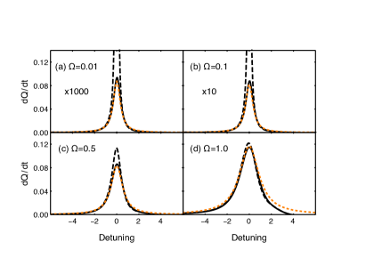
Figure 2: Rates of heat absorption from the phonon bath, as a function of the detuning $\delta=\omega_{l}-E_{0}$ of the driving laser from resonance, for four different Rabi frequencies. For each Rabi frequency we show results computed using the full Bloch-Redfield equation (solid black curve), a phenomenological Lindblad equation (dashed orange curve), and the Bloch-Redfield equation in the secular approximation without the principal value terms (dashed black curve). The Rabi frequencies $\Omega$ are: (a) 0.01, (b) 0.1, (c) 0.5, and (d) 1.0.

Fig. 2 shows the calculating cooling power as a function of the detuning, $\delta$, for four different strengths of driving field. The different curves are computed using the full Bloch-Redfield equation, (7), the phenomenological Lindblad form, Eq. (17), and the secular Bloch-Redfield equation, (10). Considering first weak driving, in Fig. 2a, we see that the Bloch-Redfield and phenomenological theories agree well, and give a cooling profile which appears to be Lorentzian, as one would expect. While the secular Bloch-Redfield equation agrees away from the resonance, we see that it fails close to it, massively overestimating the cooling power. The secular approximation is, of course, not justified here, because there are near degeneracies in the Hamiltonian. Nonetheless, the level of disagreement seems surprising, given the agreement away from resonance.

In the converse, strong-driving region, Fig. 2d, all three methods give similar results. However, there is a noticeable difference on the high-energy side of the transition, with the phemenological theory giving, as before, a Lorentzian profile, while the other theories predict the heat current drops off more rapidly, and indeed switches direction, from cooling to heating, in the range of detunings shown.

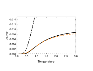
Figure 3: Rate of heat absorption from the phonon bath, as a function of temperature, for the different approaches. Results are shown for weak driving, $\Omega=0.1$, at resonance, $\delta=0$. The heat current is computed using the full Bloch-Redfield equation (solid black curve), the phenomenological Lindblad equation (dashed orange curve), and the Bloch-Redfield equation in the secular approximation without the principal value terms (dashed black curve).

Fig. 3 shows the temperature dependence of the cooling power for weak resonant driving. As noted above, the secular approximation is inappropriate in this regime and massively overestimates the cooling power. The other theories agree closely and appear physically reasonable, predicting that the cooling power drops rapidly once the temperature is lowered below the splitting $E_{\mathrm{man}}$. This is the expected physical behaviour for laser cooling in a discrete level structure, caused by the vanishing of the phonon occupation at temperatures much less than $E_{\mathrm{man}}$. The precise behaviour at very low temperatures is not relevant to laser cooling, since it is not expected to operate there. Nonetheless it may be noted that, for these parameters, the Bloch-Redfield theory predicts a very small but negative cooling power, i.e. net heating, at very low temperatures ($T<0.38$). However, this is an approximate theory whose accuracy is not sufficient to discern the true behaviour of the heat current in this regime. Indeed, we find that at these very low temperatures the theory does not predict a physical density matrix, giving one which has a negative, albeit very small, eigenvalue.

In Fig. 4 we compare between the cooling spectra predicted by the full Bloch-Redfield equation with those obtained from the exact numerical method Popovic et al. (2021). The numerical method simulates the time-evolution of the open quantum system, using discrete timesteps. For these simulations we have taken a timestep $dt=0.05$, and computed the heat current, at a time $t=30.0$, from the difference in the heat transfer at two times. The mean heat transfer is computed by evaluating the annotated reduced density matrix, $\rho_{u,S}(t)$, and computing the finite difference approximation to the derivative in Eq. (15) from the values of $\operatorname{Tr}\rho_{u,S}(t)$ at $u=0.05$ and $u=0.0$. The numerical accuracy and convergence of these simulations involves two further parameters: a maximum number of timesteps retained in the influence functional, $K$, and a cut-off paramater controlling the truncation of the singular-value decompositions. We take $K=100$, and use a cut-off of $10^{-7}$.

We see from Fig. 4 that the Bloch-Redfield equation is in excellent agreement with the numerical results. The non-Lorentzian behaviour of the cooling profile on the high-energy side, predicted by the full Bloch-Redfield and secular equations, is present. There is a slight overestimate of the cooling power in the tails of the profiles, which we believe is because the heat current has not yet reached its steady-state value at those small values of the cooling power.

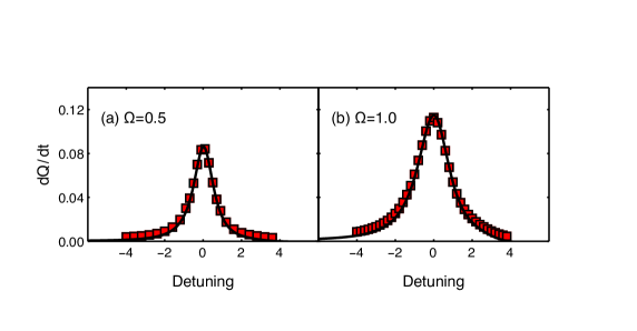
Figure 4: Heat absorption rates, as a function of the detuning, computed using the full Bloch-Redfield equation (solid black curves) and a numerically exact method (red squares), for two different Rabi frequencies. The Rabi frequencies $\Omega$ are (a) 0.5 and (b) 1.0.

4 Discussion

Figs. 2 and 4 suggest that the full Bloch-Redfield equation gives an accurate account of the cooling profile, in both the weak- and strong-driving cases. In the weak-driving case it agrees with the phenomenological theory, which is well-justified for weak-driving, while in the strong-driving case it agrees with the secular theory, which is well-justified there. Furthermore, it agrees with exact numerical results, in the strong-driving regime where such simulations are possible. Thus the Bloch-Redfield equation allows a complete treatment of both regimes, using a single equation. This conclusion is similar to previous conclusions on the dynamics and thermodynamics of other open quantum systems, where the Bloch-Redfield equation has similarly been argued to provide the most accurate description Eastham et al. (2016); Hartmann and Strunz (2020); Purkayastha et al. (2016); Kilgour and Segal (2018); Liu and Segal (2021). This is in spite of the possibility that it produces unphysical density matrices with non-positive eigenvalues. That possibility does not occur in our results, except at very low temperatures where laser cooling would not, in any case, be expected to operate.

In previous works it has been noted that the secular approximation does not allow for the presence of bath-induced or noise-induced coherence Tscherbul and Brumer (2014) in multilevel systems where near-degenerate levels have different couplings to the bath Eastham et al. (2016). This phenomenon can play an important role for the heat currents, as has been pointed out previously for quantum absorption refrigerators Kilgour and Segal (2018); Liu and Segal (2021). Its significance in our case can be seen by comparing the secular result (where there is no bath-induced coherence) and the Bloch-Redfield result (where there is) in Fig. 2. When $\delta=0,\Omega=0$ our Hamiltonian has two degenerate eigenstates, but the form of those eigenstates depends on how the limit is taken: for $\delta=0,\Omega\neq 0$ they are $|\pm\rangle=|g_{u}\rangle\pm|e\rangle$, but for $\Omega=0,\delta\neq 0$ they are $|g_{u}\rangle$ and $|e\rangle$. The naive form of secular approximation in Eq. (10) produces a dissipator which populates the states $|+\rangle$ and $|-\rangle$, and destroys coherences between them. However, we observe that the phonon bath couples only to $|g_{u}\rangle\propto|+\rangle+|-\rangle$, and not to $|e\rangle\propto|+\rangle-|-\rangle$, so in the weak-driving case the correct dissipator should affect the population of the first combination, while leaving that of the second undamped. This means that there are undamped coherences in the $|\pm\rangle$ basis, which survive in the steady-state Eastham et al. (2016), and produce corrections to the heat currents relative to the results of the secular approximation.

Conceptualization, methodology, software, analysis, investigation, C.M., L.T.T., P.E. Writing — original draft preparation, P.E.; writing—review and editing, C.M., L.T.T.; visualization, supervision, P.E. All authors have read and agreed to the published version of the manuscript.

This research was funded by the Irish Research Council grant number GOIPG/2017/1091. Some calculations were performed on the Boyle cluster maintained by the Trinity Centre for High Performance Computing. This cluster was funded through grants from the European Research Council and Science Foundation Ireland.

The data generated in this study are available in Zenodo.