PDF bias and flavor dependence in TMD distributions

Abstract

Transverse momentum dependent (TMD) distributions match collinear parton density functions (PDF) in the limit of small transverse distances, which is accounted for by global extractions of TMD distributions. We study the influence of the collinear PDF value and uncertainties on the determination of unpolarized TMD distributions and the description of Drell-Yan (DY) and Z-boson production measurements at low transverse momenta. We take into account, for the first time, flavor-dependent non-perturbative TMD profiles. We carry out a Bayesian analysis to incorporate the propagation of PDF uncertainties into TMD extractions. We find that collinear PDF uncertainties and non-perturbative TMD flavor dependence are both essential to obtain reliable TMD determinations, and should be included in future global analyses.

1 Introduction

While determinations of the proton’s collinear parton distribution functions (PDFs) Kovarik:2019xvh from fits to experimental data have been carried out for four decades, and PDFs are nowadays known with high precision, the systematic investigation of the transverse momentum dependent (TMD) Angeles-Martinez:2015sea distribution functions has started much more recently. In the last few years determinations of TMD distributions Aybat:2011zv from fits to experimental data have been performed in the context of low transverse momentum Drell-Yan (DY) production and semi-inclusive deep inelastic scattering (SIDIS) Scimemi:2019cmh ; Bertone:2019nxa ; Scimemi:2017etj ; Bacchetta:2019sam ; Bacchetta:2017gcc , small-$x$ deep inelastic scattering Hautmann:2013tba , nonlinear TMD evolution Kotko:2017oxg , and parton branching BermudezMartinez:2018fsv . The results are collected in the public library TMDlib Abdulov:2021ivr ; Hautmann:2014kza , similarly to LHAPDF for the case of PDF.

A physical cross section $\sigma$ with hard scale $Q$ and measured transverse momentum $q_{T}\ll Q$ is described in terms of TMD distributions by a factorization formula with the schematic form (up to power corrections in $q_{T}/Q$ and $\Lambda_{\rm{QCD}}/Q$)

$${{d\sigma}\over{dq_{T}^{2}}}=\sum_{i,j}\int d^{2}b\ e^{ib\cdot q_{T}}\sigma^{(0)}_{ij}f_{1,i\leftarrow h1}(x_{1},b;\mu,\zeta_{1})f_{1,j\leftarrow h2}(x_{2},b;\mu,\zeta_{2}),$$ (1)

where $b$ is the transverse distance Fourier conjugate to transverse momentum, $\sigma^{(0)}_{ij}$ are perturbatively calculable partonic cross sections, and $f_{i}$ and $f_{j}$ are TMD parton distributions. These depend on the mass and rapidity scales $\mu$ and $\zeta$ through appropriate evolution equations, involving both perturbative and non-perturbative (NP) components, and are to be determined from fits to experiment.

Current fits of TMD distributions from DY and SIDIS measurements are performed by using not only the TMD factorization and evolution framework but also additional inputs which exploit the relationship between TMD distributions and the collinear PDFs. These relations follow from the operator product expansion (OPE) applied to the TMD operator. The OPE expresses the TMD distributions at small distances $b$ in terms of PDFs via perturbatively calculable coefficients, with power corrections in $b$, as follows

$$f_{1,f\leftarrow h}(x,b;\mu,\zeta)=\sum_{f^{\prime}}\int_{x}^{1}\frac{dy}{y}C_{f\leftarrow f^{\prime}}\left(y,b;\mu,\zeta\right)q_{f^{\prime}}\left(\frac{x}{y},\mu\right)+O(b^{2}),$$ (2)

where $f_{i}(x,b;\mu,\zeta)$ is the TMD distribution, $q_{j}(x,\mu)$ is the PDF, $C_{ij}$ are the Wilson coefficient functions, $\mu$ and $\zeta$ are factorization scales, the subscripts $f$ and $f^{\prime}$ indicate parton flavors, and the last term on the right hand side is the power suppressed correction at small $b$. An expansion such as eq. (2) is used, for instance, in the context of precision studies of the DY transverse momentum $q_{T}$ spectrum at the Large Hadron Collider (LHC) Lhcew:2022pt to carry out comparisons of small-$q_{T}$ logarithmic resummations between computer codes based on TMD distributions (e.g., artemide Scimemi:2017etj , NangaParbat Bacchetta:2019sam ) and computer codes which perform perturbative small-$q_{T}$ resummation without systematically introducing TMD distributions (e.g., DYturbo Camarda:2019zyx ; Camarda:2021ict , reSolve Coradeschi:2017zzw ; Accomando:2019ahs , Radish Bizon:2018foh ; Chen:2022cgv , SCETlib Ebert:2020dfc ; Ebert:2016gcn , CuTe Becher:2020ugp ).

To carry out TMD fits an ansatz is made for the NP TMD distribution at large $b$, where the power corrections to OPE become sizeable. This is of the form Bacchetta:2017gcc ; Scimemi:2017etj ; Bacchetta:2019sam ; Bertone:2019nxa ; Scimemi:2019cmh ; Vladimirov:2019bfa ; Bury:2020vhj ; Echevarria:2020hpy

$$f_{1,f\leftarrow h}(x,b;\mu,\zeta)=\sum_{f^{\prime}}\int_{x}^{1}\frac{dy}{y}C_{f\leftarrow f^{\prime}}\left(y,b;\mu,\zeta\right)q_{f^{\prime}}\left(\frac{x}{y},\mu\right)f_{\text{NP}}^{f}(x,b),$$ (3)

where $f_{\text{NP}}^{f}$ is a function which contains power corrections to eq. (2), behaves as $f_{\text{NP}}^{f}(x,b)\sim 1+O(b^{2})$ for $b\to 0$, and is to be fitted to experimental data. This ansatz reproduces eq. (2) for $b\to 0$ but allows for modifications at finite $b$. Current fits determine the NP TMD distributions, once a choice is made for the collinear PDFs in eq. (3).

The PDF choice in eqn.(3) determines the value of TMD distribution and influences $f_{\text{NP}}$ (we address this as PDF bias). Consequently, the extraction based solely on the central value of PDF are incomplete, and PDF uncertainties should be incorporated. The way the PDF error propagates has nontrivial consequences which have not been studied in the literature so far. The purpose of this work is to develop methods for addressing these issues, to critically assess the current status of phenomenological analyses based on TMD factorization and OPE expansion, and to perform the first systematic investigation of the role of PDF bias in TMD determinations.

To this end, we take PDF sets HERA20 Abramowicz:2015mha , NNPDF3.1 Ball:2017nwa , CT18 Hou:2019efy and MSHT20 Bailey:2020ooq as representatives of different methodological approaches at next-to-next-to-leading order (NNLO); we use the implementation of the TMD factorization formula as in refs. Scimemi:2019cmh ; Hautmann:2020cyp to perform fits of experimental measurements for unpolarized DY and $Z$-boson production at small $q_{T}$, from fixed-target to LHC energies; we devise and implement a Bayesian procedure to propagate the PDF uncertainties, for each PDF set, to TMD extractions. This enables us to present results for the fitted NP TMD distributions which display, for the first time, both experimental and PDF uncertainties. We find that the role of the collinear PDFs is very significant in current TMD phenomenology. We discuss the issues associated with the combination of the different sources of TMD uncertainty, and propose an approach based on the bootstrapping method.

An important aspect addressed by our work concerns the physical properties of the NP distributions $f_{\text{NP}}^{f}$ in eq. (3). The fits based on TMD factorization and evolution which have so far been performed in the literature have assumed flavor-independent parameterizations for $f_{\text{NP}}^{f}$, with the flavor dependence solely in collinear PDFs, motivated by the belief that available data have little sensitivity to TMD flavor structure. In this work we go beyond this assumption and include flavor dependence in the NP TMD distributions. We find that the the inclusion of TMD flavor dependence improves the quality of the fits significantly, leading both to a better agreement of theory with data and to more consistent results among different collinear PDF sets. For each set, we examine the distribution of $\chi^{2}$ values over PDF replicas. We demonstrate that the spread in the $\chi^{2}$ distribution among replicas is much reduced with flavor-dependent TMD compared to the flavor-independent case, and that this conclusion applies consistently across collinear sets.

A complete treatment of the problems studied in this paper should eventually involve simultaneous fits of PDF and TMD distributions, requiring much more computational power than is available to us at present. The analysis presented in this paper underlines essential elements which should be included in future TMD studies.

The article is structured as follows. Sec. 2 provides basic theoretical inputs and notation, and presents the flavor dependent model used for $f_{\rm NP}^{f}$. Sec. 3 describes the data used in the analysis. The statistical methods are reported in sec. 4. Sec. 5 presents the results of the fits and the discussion of their consequences. We give conclusions in sec. 6. We collect further details on the fits in the appendix.

2 Theory inputs

In this section we summarize the basic theoretical inputs of our analysis: i) TMD factorization formula for the DY cross section and evolution equations for the TMD distributions, and ii) models for the non-perturbative contributions to TMD factorization and evolution formulas.

The new element in this section is the flavor-dependent TMD profile in eq. (7): to our knowledge, flavor dependence of the TMD has not been considered before in the context of DY or SIDIS fits including TMD evolution.

2.1 DY factorization formula

The TMD factorized expression for the differential cross-section of the DY process $h_{1}+h_{2}\to\gamma^{*}/Z(\to\ell^{+}\ell^{-})+X$ in the low transverse momentum region can be written as Collins:2011zzd ; Collins:1984kg

$$\frac{d\sigma}{dQ^{2}dyd\bm{q}_{T}^{2}} = \sum_{f}\sigma_{0}\int_{0}^{\infty}db\,bJ_{0}(bq_{T})H(Q,\mu)f_{1,f\leftarrow h_{1}}(x_{1},b;\mu,\zeta_{1})f_{1,\bar{f}\leftarrow h_{2}}(x_{2},b;\mu,\zeta_{2})$$

$$\qquad+{\cal O}\left({q_{T}/Q}\right)+{\cal O}\left({\Lambda_{\rm{QCD}}/Q}\right).$$

Here $Q^{2}$ is the invariant mass of the vector boson, $\bm{q}_{T}$ is the transverse component of its momentum (relative to the scattering plane), and $\Lambda_{\rm{QCD}}$ is the characteristic hadronic scale. The index $f$ runs over all active quark flavors. The distribution $f_{1}$ is the unpolarized TMDPDF, depending on the lightcone momentum fraction $x$, transverse distance $b$, mass and rapidity scales $\mu$ and $\zeta$; $\sigma_{0}$ is the leading-order DY cross section, $H$ is the perturbative hard factor containing higher-order corrections, and $J_{0}$ is the Bessel function. The formula is valid up to power-suppressed corrections in $q_{T}/Q$ and $\Lambda_{\rm{QCD}}/Q$, indicated in the second line of eq. (2.1). The DY factorization formula (2.1) has been rederived in Becher:2010tm ; Echevarria:2011epo ; Chiu:2012ir . We use its implementation as given in refs. Scimemi:2017etj ; Scimemi:2018xaf ; Scimemi:2019cmh ; Vladimirov:2019bfa ; Bertone:2019nxa ; Gutierrez-Reyes:2019vbx ; Hautmann:2020cyp ; Gutierrez-Reyes:2020ouu ; Bury:2020vhj ; Moos:2020wvd ; Vladimirov:2021hdn .

The evolution of TMD distributions in mass and rapidity is given by the pair of equations

$$\mu^{2}\frac{\partial f_{1,f\leftarrow h}(x,b;\mu,\zeta)}{\partial\mu^{2}} =\left(\Gamma_{\rm cusp}\ln\frac{\mu^{2}}{\zeta}-\gamma_{V}(\mu)\right)f_{1,f\leftarrow h}(x,b;\mu,\zeta),$$

$$\zeta\frac{\partial f_{1,f\leftarrow h}(x,b;\mu,\zeta)}{\partial\zeta} =-{\cal D}(b,\mu)f_{1,f\leftarrow h}(x,b;\mu,\zeta),$$ (5)

where $\Gamma_{\rm cusp}$ is the anomalous dimension for the cusp of light-like Wilson lines, $\gamma_{V}$ is the anomalous dimension of the quark vector form factor and $\mathcal{D}$ is the Collins-Soper (CS) kernel Collins:1981uk ; Collins:1981va . We will use the solution of the evolution equations according to the $\zeta$-prescription Scimemi:2017etj ; Scimemi:2018xaf ; Vladimirov:2019bfa ; Scimemi:2019cmh . Using the expansion (3), this solution is expressed in terms of PDFs, $f_{\text{NP}}^{f}$ and the matching coefficients Echevarria:2016scs ; Luo:2020epw ; Luo:2019szz ; Ebert:2020yqt .

The perturbative orders in the strong coupling $\alpha_{s}$ which will be used in the calculations presented in the following sections are summarised in tab. 1 for each element of the cross section. The definition of $\mathcal{D}_{\text{resum}}$ is given in the next subsection. The resulting cross section corresponds to the logarithmic order NNLL^′ according to the terminology in Lhcew:2022pt .

$H$	$C_{f\leftarrow f^{\prime}}$	$\Gamma_{\rm cusp}$	$\gamma_{V}$	$\mathcal{D}_{\text{resum}}$	$\alpha_{s}$ running $\&$ PDF evolution
$\alpha_{s}^{2}$	$\alpha_{s}^{2}$	$\alpha_{s}^{3}$	$\alpha_{s}^{2}$	$\alpha_{s}^{2}$	NNLO

Table 1: Summary of the perturbative orders used for each element of the cross section.

2.2 Non-perturbative models

The NP content of the DY differential cross section is encoded in two functions: the CS kernel $\mathcal{D}$ in eq. (2.1) and the TMD distribution $f_{\text{NP}}^{f}$ in eq. (3).

We write the CS kernel as

$$\mathcal{D}(b,\mu)=\mathcal{D}_{\text{resum}}(b^{*}(b),\mu)+c_{0}bb^{*}(b)\,,$$ (6)

where the first term $\mathcal{D}_{\text{resum}}$ on the right hand side is the resummed expression for $\mathcal{D}$ at small $b$ Echevarria:2012pw with NNLO perturbative coefficients Echevarria:2015byo ; Vladimirov:2016dll , while the second term is the non-perturbative model, given in terms of $b^{*}(b)=b/\sqrt{1+(b/B_{\rm NP})^{2}}$, with parameters $c_{0}$ and $B_{\rm NP}$ to be determined from data. Motivated by the results of the fit Scimemi:2019cmh , for simplicity in what follows we will take a fixed value $B_{\rm NP}=2$ GeV^-1 and leave only $c_{0}$ to be fitted to data. The model in eq. (6) is linear at $b\to\infty$: this ansatz is partially supported by the studies Vladimirov:2020umg ; Collins:2014jpa and lattice computations LatticeParton:2020uhz ; Schlemmer:2021aij ; Shanahan:2021tst , and it has already been used in ref. Scimemi:2019cmh . In refs. Hautmann:2020cyp ; Hautmann:2021ovt alternative models, with quadratic asymptotic behavior (as in the studies Konychev:2005iy ; Landry:2002ix ; Landry:1999an ) and with constant asymptotic behavior (in the spirit of the $s$-channel picture Hautmann:2007cx ; Hautmann:2000pw ; Hautmann:1999ui ), have also been analyzed. Corresponding investigations based on these different asymptotic behaviors are left to future work.

The main new feature of the NP treatment in the present analysis concerns the TMD distribution $f_{\text{NP}}^{f}$. We include flavor dependence in the TMD profile, and take the parameterization

$$f_{\text{NP}}^{f}=\exp\left(-\frac{(1-x)\lambda_{1}^{f}+x\lambda_{2}^{f}}{\sqrt{1+\lambda_{0}x^{2}b^{2}}}b^{2}\right),$$ (7)

with $\lambda_{1,2}^{f}>0$ and $\lambda_{0}>0$. The model is characterized by an exponential asymptotic fall-off at $b\to\infty$ and a Gaussian-like shape at intermediate $b$ Landry:2002ix ; Guzzi:2013aja ; Schweitzer:2010tt ; Schweitzer:2012hh ; Scimemi:2016ffw ; Scimemi:2017etj . While the parameter $\lambda_{0}$ is taken to be universal for all flavors, the parameters $\lambda_{1,2}$ are taken to be flavor dependent. We distinguish $u$, $d$, $\bar{u}$, $\bar{d}$ and $sea$ cases, where $sea$ is used for $(s,\bar{s},c,\bar{c},b,\bar{b})$ flavors. In total we have 11 free parameters. Since the parameters $\lambda_{1,2}$ are almost uncorrelated across flavors, the presence of unnecessary fitting parameters (i.e. not well restricted in a particular setup) does not lead to an overfit.

The numerical implementation is made with artemide Scimemi:2017etj , which can be found in open-access repository web . The PDF values and their evolution are taken from LHAPDF Buckley:2014ana . Artemide is a FORTRAN code, with a Python interface. The evaluation of a single DY-cross-section point includes two convolutions of PDFs, Hankel type integrals and three integrations over the phase space. Additionally, for some measurement one needs to take into account fiducial cuts. The artemide code is optimized for such computations, and it uses various numerical tricks, such as precomputed grids, specially optimized integration algorithms and parallel evaluation. Even so the computation of one value of $\chi^{2}$ for the data set takes from 30 seconds to a few minutes, depending on the PDF input, NP parameters, experimental fiducial cuts and hardware. Therefore, a single minimisation procedure (made with the help of the iMINUIT package iminuit ) requires typically a few dozen hours on an average computer.

3 TMD data sets

3.1 Complete data set

The complete data set used in this study is given in tab. 2. We restrict the fit to data points in the low transverse momentum region by implementing the cut $q_{T}/Q<0.25$ . In addition we implement an extra cutting rule for the very precise data typically encountered at LHC. Given a data point $p(1\pm\sigma)$, with $p$ being the central value and $\sigma$ its uncorrelated relative uncertainty, corresponding to some values of $q_{T}$ and $Q$, we include it in the fit only if

$$\delta\equiv\frac{\langle q_{T}\rangle}{\langle Q\rangle}<0.1,\qquad\text{or}\qquad\delta<0.25\quad\text{if}\quad\delta^{2}<\sigma.$$ (8)

In other words, if the (uncorrelated) experimental uncertainty of a given data point is smaller than the theoretical uncertainty associated to the expected size of the power corrections, we drop it from the fit.

The resulting data set in tab. 2 contains 507 data points, and spans a wide range in mass, from $Q=4$ GeV to $Q=150$ GeV, and in $x$, from $x\sim 0.5\cdot 10^{-4}$ to $x\sim 1$. The data roughly split into low-energy and high-energy points. The low-energy subset contains data from fixed target experiments E288 Ito:1980ev , E605 Moreno:1990sf and E772 McGaughey:1994dx , and PHENIX Aidala:2018ajl . The high-energy subset contains data from the neutral current DY (Z/$\gamma$-boson) measured at the Tevatron Affolder:1999jh ; Aaltonen:2012fi ; Abbott:1999wk ; Abazov:2007ac ; Abazov:2010kn and LHC Aad:2014xaa ; Aad:2015auj ; Chatrchyan:2011wt ; Khachatryan:2016nbe ; CMS:2019raw ; Aaij:2015gna ; Aaij:2015zlq ; Aaij:2016mgv . The subsets have similar number of points but those in the high-energy subset are one order of magnitude more precise. The data that we are using are very similar to those included in previous fits Bertone:2019nxa ; Scimemi:2019cmh ; Bacchetta:2019sam but we consider also the recent CMS Z-boson production data at 13 TeV CMS:2019raw .

The treatment of particular aspects of the measurements such as bin-integration, nuclear modifications and normalization conditions are as in ref. Scimemi:2019cmh and we refer to it for extra details. Notice that we use the absolute values of the cross-section, whenever available, and perform the full bin-integration to accurately incorporate the phase-space effects. The only modification of the data treatment in comparison to Scimemi:2019cmh is the splitting of the low-energy measurements (namely E288 at $E_{\text{beam}}=300$ and $400$ GeV, E605 and E772) into two independent subsets below and above the $\Upsilon$-resonance. This allows us to treat the normalization error independently for these energies. The reason for doing this is a possible inconsistency between these energy regions inside the measurements, which leads to tensions.

Experiment	ref.	$\sqrt{s}$ [GeV]	$Q$ [GeV]	$y$/$x_{F}$	$N_{\rm pt}$after TMD cuts	$N_{\rm pt}$ in red.set
E288 (200)	Ito:1980ev	19.4	4 - 9 in 1 GeV bins∗	$0.1<x_{F}<0.7$	43	39
E288 (300)	Ito:1980ev	23.8	4 - 12 in 1 GeV bins∗	$-0.09<x_{F}<0.51$	53	53
E288 (400)	Ito:1980ev	27.4	5 - 14 in 1 GeV bins∗	$-0.27<x_{F}<0.33$	76	76
E605	Moreno:1990sf	38.8	7 - 18 in 5 bins∗	$-0.1<x_{F}<0.2$	53	53
E772	McGaughey:1994dx	38.8	5 - 15 in 8 bins∗	$0.1<x_{F}<0.3$	35	24
PHENIX	Aidala:2018ajl	200	4.8 - 8.2	$1.2<y<2.2$	3	2
CDF (run1)	Affolder:1999jh	1800	66 - 116	inclusive	33	0
CDF (run2)	Aaltonen:2012fi	1960	66 - 116	inclusive	39	15
D0 (run1)	Abbott:1999wk	1800	75 - 105	inclusive	16	0
D0 (run2)	Abazov:2007ac	1960	70 - 110	inclusive	8	0
D0 (run2)μ	Abazov:2010kn	1960	65 - 115	inclusive	3	3
ATLAS (7TeV)	Aad:2014xaa	7000	66 - 116	$|y|<1$ $1<|y|<2$ $2<|y|<2.4$	15	0
ATLAS (8TeV)	Aad:2015auj	8000	66 - 116	$|y|<2.4$ in 6 bins	30	30
ATLAS (8TeV)	Aad:2015auj	8000	46 - 66	$|y|<2.4$	3	3
ATLAS (8TeV)	Aad:2015auj	8000	116 - 150	$|y|<2.4$	7	0
CMS (7TeV)	Chatrchyan:2011wt	7000	60 - 120	$|y|<2.1$	8	0
CMS (8TeV)	Khachatryan:2016nbe	8000	60 - 120	$|y|<2.1$	8	0
CMS (13TeV)	CMS:2019raw	13000	76 - 106	$|y|<2.4$ in 6 bins	50	0∗∗
LHCb (7TeV)	Aaij:2015gna	7000	60 - 120	$2<y<4.5$	8	4
LHCb (8TeV)	Aaij:2015zlq	8000	60 - 120	$2<y<4.5$	7	7
LHCb (13TeV)	Aaij:2016mgv	13000	60 - 120	$2<y<4.5$	9	0
Total					507	309

*Bins with $9\lesssim Q\lesssim 11$ are omitted due to the $\Upsilon$ resonance.

Table 2: Summary table for the data included in the fit. For each data set we report: reference publication, centre-of-mass energy, coverage in $Q$ and $y$ or $x_{F}$, possible cuts on the fiducial region, and number of data points that survive the cut of eq. (8).

3.2 Reduced data set

Given the data set defined above, we observe that the sensitivity to NP parameters of the TMD distributions varies strongly within the data set. For instance, data points with $q_{T}\sim$ 15-25 GeV have little power in constraining NP parameters, irrespective of their precision, because they are deeply inside the resummation region, where the Hankel integral is dominated by the $b\ll 1$GeV^-1 contribution, and determined by PDF values only. The inclusion of these points in the fit is not harmful but rather time consuming. To speed up the fitting procedure, we have considered a reduced set of data points.

To identify the relevant points for the TMD extraction, we tested the sensitivity of the theory prediction to the variation of NP parameters, and included only the points that are sensitive to the variation. Given a NP parameter $p$, we compute the cross-section for several values of $p$ distributed in the range $p\pm\delta p$, and compute the sensitivity coefficient between $p$ and the cross-section, by the formula

$$s_{\sigma,p}=\frac{\langle\sigma\cdot p\rangle-\langle\sigma\rangle\langle p\rangle}{\Delta\sigma\,\delta p},$$ (9)

where $\Delta\sigma$ is the uncorrelated experimental uncertainty of the point. The sensitivity coefficient indicates how strongly a prediction for a data point depends on the parameter $p$. E.g., $s_{\sigma,p}=1$ means that the variation of $p$ by $\delta p$ gives rise to a variation in the theory prediction equal to the experimental uncertainty.

We computed the sensitivity coefficient for each point in the data set and for each parameter of our NP ansatz. The values of $\delta p$ are taken using the Hesse estimation for its uncertainty multiplied by a factor 5. Points with $s>0.4$ for at least one parameter were included in the reduced set. This test was run for each of the PDF sets that we studied, and the union of data was taken. This provided us with a very conservative selection of impacting data.

Afterwards, we excluded the sets with too few points, such as LHCb (13 TeV) (1 surviving point) and CDF (run1) (5 points remaining out of 33). Additionally, we excluded the ATLAS (7 TeV) measurement since it has shown an anomalous behaviour and provides significant tension with other similar measurements.

The reduced set contains 309 data points. Most excluded points are from the region characterized by high energy and high $q_{T}$. The low-energy subset, in contrast, is very sensitive to the NP input and lost only 15 points due to their large error bands. We have checked, by evaluating several random cases, that the minimum of the $\chi^{2}$ of the reduced set almost coincides (up to 2 digits) with the minimum of $\chi^{2}$ of the complete set.

4 Statistical framework

The central point of the present study is the impact of the PDF uncertainty on the extraction of TMD distributions. Therefore, we distinguish two sources of uncertainties: $i)$ the experimental uncertainties and $ii)$ the uncertainty of the collinear PDFs. These have different nature, and could not be easily combined together. In fact, the best approach to account for the PDF uncertainty would be a simultaneous global fit of collinear PDF and TMDPDF, which is challenging. In the present work, we use the strategy of combining PDF and experimental uncertainty based on Bayesian statistics, described in this section.

4.1 Definition of the $\chi^{2}$-function

Our main tool is the $\chi^{2}$-test function, which estimates the goodness of a theory prediction. It is defined as

$$\chi^{2}=\sum_{i,j=1}^{n}\left(m_{i}-t_{i}\right)V_{ij}^{-1}\left(m_{j}-t_{j}\right)\,,$$ (10)

where $i$ and $j$ enumerate points of the data set. For the $i$th point, $t_{i}$ is the corresponding theoretical prediction, $m_{i}$ is the experimental value, and all the information about the uncertainties for individual data points and the relation between them is given by the covariance matrix $V_{ij}$. The definition of $V_{ij}$ is crucial for an adequate analysis of the data and interpretation of the results. Its construction distinguishes two types of uncertainties: uncorrelated and correlated. In general, the $i$th point is given as

$$m_{i}\pm\sigma_{i,\text{stat}}\pm\sigma_{i,\text{unc}}\pm\sigma_{i,\text{corr}}^{(1)}\pm\dots\pm\sigma_{i,\text{corr}}^{(k)}\,.$$ (11)

Here $\sigma_{i,\text{stat}}$ and $\sigma_{i,\text{unc}}$ are the uncorrelated statistical and systematic uncertainties, respectively, that estimate the degree of knowledge of the $i$th data point regardless of all other data in the set. The correlated uncertainties $\sigma_{i,\text{corr}}^{(k)}$ (with $k=1,...,n$) estimate the relation between the statistical fluctuations of the $i$th point and all others in the set. The covariance matrix $V_{ij}$ can be written as Ball:2008by ; Ball:2012wy

$$V_{ij}=\left(\sigma_{i,\text{stat}}^{2}+\sigma_{i,\text{unc}}^{2}\right)\delta_{ij}+\sum_{l=1}^{k}\sigma_{i,\text{corr}}^{(l)}\sigma_{j,\text{corr}}^{(l)},.$$ (12)

Using this expression in the computation of eq. (10) allows us to obtain a reliable estimation of data-to-theory agreement, while taking into account the nature of experimental uncertainties.

The minimum of the $\chi^{2}$-test function determines the preferred values of the NP parameters $\lambda$, which in turn characterize the preferred shape of TMD distributions. The fit procedure consists in the minimization of $\chi^{2}$, which is performed with the iMinuit package iminuit .

In fitting a multivariate function one usually finds several sets of parameters giving numerous local minima of the function. Some of these give mathematically correct but physically unsound results, and therefore a strategy should be implemented to discard them. The MINUIT algorithm can handle the problem of choosing the correct minimum, unless the minima are significantly separated in the parameter space and/or the step (the amount by which the parameters move in one iteration) is too small. In our case, with the $\chi^{2}$-function depending on 11 parameters, we have faced the problem of the minimisation algorithm selecting a definitely unphysical minimum. Each occurrence is characterized by values of parameters that (almost) suppress a contribution of some flavor.

In order to disregard such contributions we introduced penalty terms into the minimisation function. The penalty function is defined as

$$P(\lambda)=10^{-2}\left(r(\lambda^{u}_{1},\lambda_{1}^{d})+r(\lambda^{u}_{2},\lambda_{2}^{d})+r(\lambda^{\bar{u}}_{1},\lambda_{1}^{\bar{d}})+r(\lambda^{\bar{u}}_{2},\lambda_{2}^{\bar{d}})\right),$$ (13)

where

$$r(a,b)=\left\{\begin{array}[]{ll}x-1,&x>1\\ 0,&\text{otherwise},\end{array}\right.\qquad\text{with}\quad x=\max\left(\frac{a}{b},\frac{b}{a}\right).$$ (16)

This function is non-zero only if the parameters of the $u$/$d$ and $\bar{u}$/$\bar{d}$ distributions differ from each other by an order of magnitude. So the minimisation was performed for the function

$$X(\text{data},\text{PDF};\lambda)=\chi^{2}+P(\lambda).$$ (17)

4.2 Input PDFs and their uncertainties

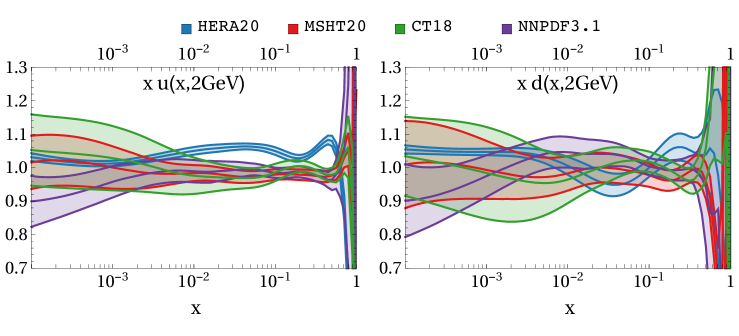
Figure 1: Comparison of the uncertainty bands of PDFs extracted by different groups for $u$ and $d$ quarks. The PDFs are weighted by an average of the central values.

Four PDF sets were used in our study, the bold font denoting the shorthand name used to identify them in the rest of this article:

• HERA20. The NNLO extraction by the H1 and ZEUS collaborations presented in ref. Abramowicz:2015mha with Hesse-like error band. The LHAPDF entry is HERAPDF20_NNLO_VAR with id = 61230.

• NNPDF31. The NNLO extraction by the NNPDF collaboration presented in ref. Ball:2017nwa with 1000 replicas at $\alpha_{s}(M_{Z})=0.118$. The LHAPDF entry is NNPDF31_nnlo_0118_1000 with id = 309000.

• CT18. The NNLO extraction by the CTEQ collaboration presented in ref. Hou:2019efy with Hesse error band. The LHAPDF entry is CT18NNLO with id = 14000.

• MSHT20. The NNLO extraction by the MSHT collaboration presented in ref. Bailey:2020ooq with Hesse error band. The LHAPDF entry is MSHT20nnlo_as118 with id = 27400.

The comparison of these PDF sets for $u$- and $d$-quarks at scale $\mu=2$ GeV is presented in fig. 1.

In what follows the analyses are done using Bayesian statistics, which requires representing the PDFs as Monte-Carlo (MC) ensembles. As the NNPDF31 set is already given in this form, no further pre-processing is required. The other three distributions have a Hessian definition of uncertainty bands. The corresponding MC ensembles are generated using the prescription given in ref. Hou:2016sho . Namely, for a distribution $f(x)$ with 68% C.I. for each eigenvector given by $f^{\pm}_{i}$ ($i=1,\dots,D$, with $f^{+}_{i}$ and $f^{-}_{i}$ the upper and lower bounds, respectively), a MC replica is generated by

$$f^{(k)}(x)=\sum_{i=1}^{D}\left(\frac{f^{+}_{i}(x)-f^{-}_{i}(x)}{2}R_{i}^{(k)}+\frac{f^{+}_{i}(x)+f^{-}_{i}(x)-2f(x)}{2}\left(R_{i}^{(k)}\right)^{2}\right),$$ (18)

where $R^{(k)}_{i}$ is a univariate random number. Using this method we generated 1000 MC replicas for HERA20, CT18 and MSHT20, which were used in the analyses. We have checked that the uncertainty bands obtained from the generated MC replicas are almost identical to the original Hesse uncertainty bands. The comparison of uncertainty bands for different PDF sets is also shown in fig.1.

4.3 Determination of uncertainties & presentation of the result

Within Bayesian statistics, the propagation of uncertainties to the free parameters is made by fitting each member of the input ensemble. Our input ensemble is generated accounting for two independent sources of uncertainty:

• EXP: The experimental uncertainty is accounted for by generating pseudo-data. A replica of the pseudo-data is obtained adding Gaussian noise to the values of the data points (and scaling the uncertainties if required). The parameters of the noise are dictated by the correlated and uncorrelated experimental uncertainties. The procedure is described in ref. Ball:2008by . We considered such 100 replicas.

• PDF: The uncertainty due to the collinear PDF is accounted for by using each PDF replica as input. We considered 1000 replicas generated as described in sec. 4.2.

The number of pseudo-data replicas is lower because the resulting uncertainty is much smaller than the one coming from the PDF distribution, as demonstrated in the following.

Fitting each member of the ensemble, we end up with the two-dimensional set $\bm{\lambda}_{ij}$, where $\bm{\lambda}$ is a 11-dimensional vector of fitting parameters (including $\lambda_{1,2}^{f}$, $\lambda_{0}$ and $c_{0}$), $i$ runs over the pseudo-data replicas, and $j$ runs over the PDF replicas. This set is distributed in accordance to the experimental and PDF uncertainties propagated through our fitting procedure. Due to the computational limitations mentioned in subsec. 2.2, calculating the full distribution with $100\times 1000=10^{5}$ members is unrealistic. To simplify the task, we consider two distributions. The first one, labeled EXP, when the replicas of the data are fitted with the central PDFs. The second one, called PDF, when the replicas of the PDFs are fitted with the central (original) data. Symbolically,

$$\{\bm{\lambda}\}_{\textbf{PDF}}=\bigcup_{j=1}^{N_{\text{rep,PDF}}}\bm{\lambda}_{0j},\qquad\{\bm{\lambda}\}_{\textbf{EXP}}=\bigcup_{i=1}^{N_{\text{rep,data}}}\bm{\lambda}_{i0},$$ (19)

where $i=0$ indicates the replica with unmodified data, and $j=0$ a replica computed with the central value of the PDF.

The PDF and EXP distributions are treated as independent. In the PDF case the distributions are also notably non-Gaussian. Therefore, we estimate the 68%C.I. for a parameter using the bootstrap method. Namely, we compute the [16%, 84%] quantile for a large number of samples and take the average interval. The results are presented as $a^{\delta a_{1}}_{\delta a_{2}}$, where $a$ is the mean value of the parameter and $\delta a$’s are the distances to the 68% C.I. boundary.

A drawback of performing the fit independently for each case is the appearance of several issues when wanting to join the two forms in a single meaningful one. The main problem is that, for some parameters, the distance between the mean values of the distributions is large. This renders impossible any naive description of a joined distribution; for example, the average value of the extracted TMDPDFs would have a large $\chi^{2}$, meaning that the corresponding TMDPDFs would not provide an adequate description of the data. Lesser, but not unimportant, problems are the correlations between individual points of TMDPDFs, and the PDF bias of the EXP case. Therefore, finally we present the central value and the 68% C.I., computed as described below.

The central value of our fit is obtained as the TMDPDF computed with the central values of the PDFs and NP parameters. The latter are computed as the weighted average of the PDF and EXP cases,

$$a=w_{\textbf{PDF}}\langle\{a\}_{\textbf{PDF}}\rangle+w_{\textbf{EXP}}\langle\{a\}_{\textbf{EXP}}\rangle,\qquad w_{i}=\frac{\sigma^{-2}_{i}}{\sigma^{-2}_{\textbf{PDF}}+\sigma^{-2}_{\textbf{EXP}}},$$ (20)

where $i=\text{\bf PDF}$ or EXP, and $\sigma_{i}=(\delta a_{1i}-\delta a_{2i})/2$ is the half-size of the 68% C.I.. In this way, the central value incorporates information from both cases but retains the knowledge of which case gives a better determination of the considered parameter. The final parameters obtained by this procedure for each PDF set are shown in tab. 5. Also, the central distribution so defined returns a reasonable value of $\chi^{2}$, which should be similar to the result that we would obtain if we had performed one joined fit. The joined 68% C.I., instead, is computed from the (equal weight) sum of replicas distributions, $\{\bm{\lambda}\}_{\text{joined}}=\{\bm{\lambda}\}_{\textbf{PDF}}\cup\{\bm{\lambda}\}_{\textbf{EXP}}$ by the bootstrap method.

The same procedure is also carried out for the values of cross-section presented in the next section. I.e. the values of cross-section are computed for all members of $\{\bm{\lambda}\}_{\textbf{PDF}}$ and $\{\bm{\lambda}\}_{\textbf{EXP}}$ resulting into $\{\sigma\}_{\textbf{PDF}}$ and $\{\sigma\}_{\textbf{EXP}}$. Then the central values and the 68% C.I. are computed using the same strategy. That is, we compute the [16%, 84%] quantile for a large number of samples drawn from the merge of PDF and EXP and take the average interval. For those parameters for which PDF and EXP coincide, the width of the sampled distributions will be narrow, the contribution to the total uncertainty closely following the one of EXP (red band in fig. 3). For those parameters for which PDF and EXP do not significantly overlap, the width of the sampled distributions will be broader, the contribution to the total uncertainty closer, but narrower, to the one from PDF (green band in fig. 3). Overall, the bootstrapping method results in an uncertainty band that resembles the one we would expect if performing the fit with simultaneous replicas of the data and the PDFs. This procedure (rather than computation of average values of parameters) accounts for the correlation between different values of TMDPDFs.

5 Results & discussion

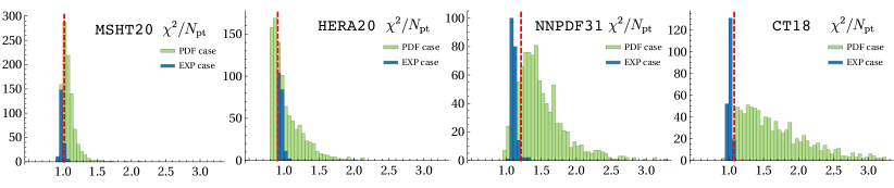
Figure 2: Distribution of $\chi^{2}$-values for the PDF and EXP cases. The red lines show the position of the final $\chi^{2}$-value.

		MSHT20	HERA20	NNPDF31	CT18
Data set	$N_{pt}$	$\chi^{2}/N_{pt}$	$\chi^{2}/N_{pt}$	$\chi^{2}/N_{pt}$	$\chi^{2}/N_{pt}$
CDF run2	15	0.96	0.68	0.65	0.82
D0 run2 ($\mu$)	3	0.50	0.59	0.55	0.52
ATLAS 8TeV 0.0<|y|<0.4	5	2.97	3.66	2.12	3.23
ATLAS 8TeV 0.4<|y|<0.8	5	2.00	1.53	4.52	3.21
ATLAS 8TeV 0.8<|y|<1.2	5	1.00	0.50	2.75	1.89
ATLAS 8TeV 1.2<|y|<1.6	5	2.25	1.61	2.49	2.72
ATLAS 8TeV 1.6<|y|<2.0	5	1.92	0.68	2.86	1.96
ATLAS 8TeV 2.0<|y|<2.4	5	1.35	1.14	1.47	1.06
ATLAS 8TeV 46<Q<66GeV	3	0.59	1.86	0.23	0.05
LHCb 7TeV	4	3.19	0.34	2.58	1.68
LHCb 8TeV	7	1.38	1.29	1.63	0.83
PHE200	2	0.32	0.36	0.43	0.27
E228-200	39	0.44	0.38	0.51	0.45
E228-300 $Q<9$GeV	43	0.77	0.56	0.89	0.55
E228-300 $Q>11$GeV	10	0.29	0.37	0.45	0.44
E228-400 $Q<9$GeV	34	2.19	1.15	1.49	1.34
E228-400 $Q>11$GeV	42	0.25	0.61	0.44	0.40
E772	24	1.58	1.92	2.51	1.56
E605 $Q<9$GeV	21	0.52	0.47	0.47	0.61
E605 $Q>11$GeV	32	0.47	0.73	1.34	0.52
Total	309	0.97	0.85	1.17	0.87

Table 3: Distribution of the values of $\chi^{2}$ for the central replica over the reduced data set in fits with different PDF inputs.

		MSHT20	HERA20	NNPDF31	CT18
Data set	$N_{pt}$	$\chi^{2}/N_{pt}$	$\chi^{2}/N_{pt}$	$\chi^{2}/N_{pt}$	$\chi^{2}/N_{pt}$
CDF run1	33	0.78	0.61	0.72	0.75
CDF run2	39	1.70	1.42	1.68	1.79
D0 run1	16	0.71	0.81	0.79	0.79
D0 run2	8	1.95	1.39	1.92	2.00
D0 run2 ($\mu$)	3	0.50	0.59	0.55	0.52
ATLAS 7TeV 0.0<|y|<1.0	5	4.06	1.94	2.12	4.21
ATLAS 7TeV 1.0<|y|<2.0	5	7.78	4.83	4.52	6.12
ATLAS 7TeV 2.0<|y|<2.4	5	2.57	2.18	3.65	2.39
ATLAS 8TeV 0.0<|y|<0.4	5	2.98	3.66	2.12	3.23
ATLAS 8TeV 0.4<|y|<0.8	5	2.00	1.53	4.52	3.21
ATLAS 8TeV 0.8<|y|<1.2	5	1.00	0.50	2.75	1.89
ATLAS 8TeV 1.2<|y|<1.6	5	2.25	1.61	2.49	2.72
ATLAS 8TeV 1.6<|y|<2.0	5	1.92	1.68	2.86	1.96
ATLAS 8TeV 2.0<|y|<2.4	5	1.35	1.14	1.47	1.06
ATLAS 8TeV 46<Q<66GeV	3	0.59	1.86	0.23	0.05
ATLAS 8TeV 116<Q<150GeV	7	0.61	1.03	0.85	0.70
CMS 7TeV	8	1.22	1.19	1.30	1.25
CMS 8TeV	8	0.78	0.77	0.75	0.78
CMS 13TeV 0.0<|y|<0.4	8	3.52	1.93	2.13	3.73
CMS 13TeV 0.4<|y|<0.8	8	1.06	0.53	0.71	1.65
CMS 13TeV 0.8<|y|<1.2	10	0.48	0.14	0.33	0.88
CMS 13TeV 1.2<|y|<1.6	11	0.62	0.33	0.47	0.86
CMS 13TeV 1.6<|y|<2.4	13	0.46	0.32	0.39	0.57
LHCb 7TeV	8	1.79	1.00	1.62	1.16
LHCb 8TeV	7	1.38	1.29	1.63	0.83
LHCb 13TeV	9	1.28	0.84	1.07	0.93
PHE200	3	0.29	0.42	0.38	0.29
E228-200	43	0.43	0.36	0.57	0.43
E228-300 $Q<9$GeV	43	0.77	0.56	0.89	0.55
E228-300 $Q>11$GeV	10	0.29	0.37	0.45	0.44
E228-400 $Q<9$GeV	34	2.19	1.15	1.49	1.34
E228-400 $Q>11$GeV	42	0.25	0.61	0.44	0.40
E772	35	1.14	1.37	1.79	1.11
E605 $Q<9$GeV	21	0.52	0.47	0.47	0.61
E605 $Q>11$GeV	32	0.47	0.73	1.34	0.52
Total	507	1.12	0.91	1.21	1.08

Table 4: Distribution of the values of $\chi^{2}$ for the central replica over the TMD data set in fits with different PDF input.

5.1 Agreement between data and theory

The individual values of $\chi^{2}$ for each experiment obtained for the reduced and complete data sets are given in tabs. 3-4, respectively. The tables also report the total $\chi^{2}$ of the fits and they show that an overall reasonable description of the data is achieved with all PDF sets. Note that the ATLAS 7 TeV data have a generally higher $\chi^{2}$ similarly to what is found also in other TMD fits Scimemi:2019cmh ; Bertone:2019nxa ; Bacchetta:2019sam ; Bacchetta:2022awv .

The $\chi^{2}$ distribution among the PDF and EXP replicas is shown in fig. 2. In general they are consistent with each other and their spread is highly reduced with respect to previous fits that use a flavor independent profile. More details on this are discussed in the appendix. This confirms the relevance of taking into account the flavor dependence of the NP TMD distributions $f_{\rm NP}^{f}$. For all cases the PDF replicas provide a much larger dispersion of the $\chi^{2}$ values than the EXP ones. The shapes of $\chi^{2}$-distributions are visibly different for different collinear PDFs, despite the resulting uncertainties in cross-section and TMDPDFs being similar. This may be due to the complexity of the corresponding parameterizations. In particular, the NNPDF and CT18 cases have more disturbed shapes of individual replicas (in comparison to HERA20 and MSHT20 cases) and consequently a larger spread of the $\chi^{2}$ distribution.

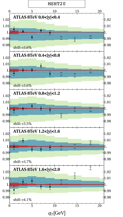
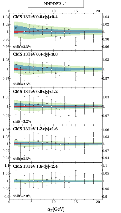
Figure 3: Example of the data description at high energy. Left panel: the ratio $d\sigma_{\text{experiment}}/d\sigma_{\text{theory}}$ for Z-boson production at 8 TeV measured by the ATLAS experiment with MSHT20. Right panel: the ratio $d\sigma_{\text{experiment}}/d\sigma_{\text{theory}}$ for Z-boson production at 13 TeV at the CMS experiment with NNPDF3.1. The red band is the EXP-uncertainty. The light-green band is the PDF-uncertainty. The blue band is the combined uncertainty. Only the filled bullets are included into the fit.

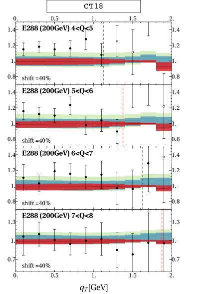
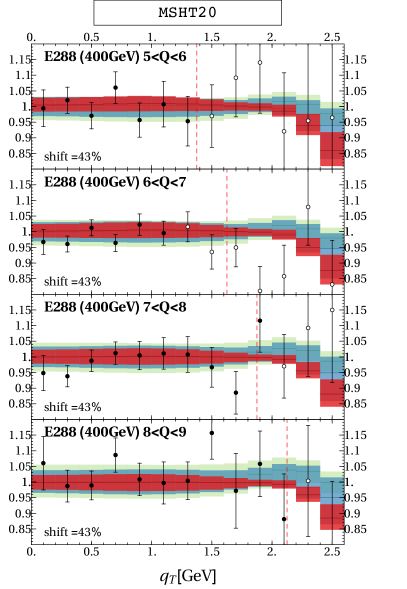
Figure 4: Example of the data description at low energy. Left panel: ratio $d\sigma_{\text{experiment}}/d\sigma_{\text{theory}}$ for the DY process at E288 experiment with 200 GeV beam-energy with CT18. Right panel: ratio $d\sigma_{\text{experiment}}/d\sigma_{\text{theory}}$ for the DY process at E288 experiment with 400 GeV beam-energy with MSHT20. Red band is the EXP-uncertainty. Light-green band is the PDF-uncertainty. The blue band is the combined uncertainty. The filled bullets are included into the fit. The dashed red vertical lines illustrate the cut $q_{T}<0.25Q$ discussed at the beginning of sec. 3.

The quality achieved in describing the data within the present fit is illustrated in figs. 3-4, for different PDF cases. Given the variety of experiments included in the fit and the number of PDF sets used, we present here only a fraction of all obtained results. We refer the interested reader to the supplementary material for the complete collection of plots. The left panel of fig. 3 illustrates the Z-boson production measured by ATLAS at $\sqrt{s}=8$ TeV Aad:2015auj , the most precise data set in our analysis. On the right panel of fig. 3, we show the comparison of the theory prediction to data for the Z-boson production measured by CMS at $\sqrt{s}=13$ TeV CMS:2019raw . Notice that these data were not included in the fit. As an example of the lowest energy measurements considered in the analysis, we present in fig. 4 the DY-process measured by the E288 experiment Ito:1980ev . In all cases, the PDF-uncertainty is larger than the EXP-uncertainty. This is especially pronounced for the high-energy measurements, for which the experimental uncertainty is small, and thus the uncertainty band is dominated by the PDF error. For $q_{T}\gtrsim 10$ GeV, the EXP-uncertainty becomes negligible. This is the resummation regime, insensitive to NP TMD effects. In a few cases (central rapidity Z-boson production with CT18, and the lowest energy bins for DY process with NNPDF3.1), the PDF and EXP bands do not overlap, illustrating an unrevealed tension in the fitting procedure.

To better appreciate the role of the PDF and EXP uncertainty bands in figs. 3-4, we next consider the theoretical uncertainty bands obtained by variation of the perturbative scales. We perform the scale variation according to the $\zeta$ prescription approach in Scimemi:2017etj ; Scimemi:2018xaf . This amounts to varying two scales, the factorization scale in the DY cross section formula and the small-$b$ matching scale in the OPE expansion of the solution of TMD evolution equations. (The small-$b$ matching scale of the CS-kernel is present in this approach but its variation is not included in the calculation.) We vary these scales by factors $c$ in the range $[0.5,2]$, and take the maximum symmetrized deviation. The resulting bands are shown in fig. 5.

We observe that the PDF uncertainty bands in fig. 3 are comparable or larger than the perturbative scale variation bands in fig. 5. This underlines that DY transverse momentum measurements in the TMD region are potentially useful to place constraints on PDFs. For this purpose one needs to employ a theoretical framework capable of describing the low transverse momentum region. One could envisage doing this in a resummation framework, formulated in terms of collinear PDF only, or in a TMD framework, in which a joined fit of both PDFs and TMDPDFs will put extra constraints on the PDFs.

5.2 Extracted TMD distributions

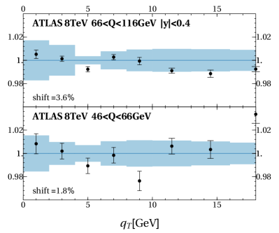
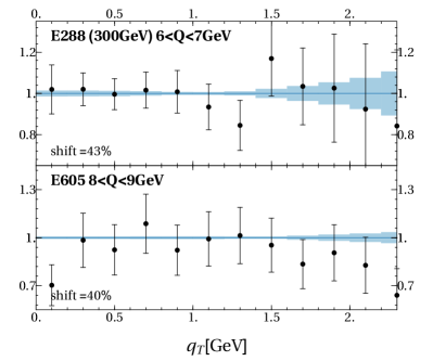
Figure 5: Scale variation band in comparison to typical data at high (left panel) and low (right panel) energies. The scale variation band is defined as the maximum symmetrized deviation from varying all scale parameters by a factor $c\in[0.5,2]$.

The values and error bars of the fitted parameters for the TMD distributions and CS kernel are given in tab. 5 and plotted in fig. 6. There, we report the bands obtained from the estimation of the PDF error (blue), the EXP error (red), and the averaged result (black). The central values for the PDF, EXP and joined cases do not coincide because they are computed with the respective replicas as explained in sec. 4.

We observe from fig. 6 that the PDF error (blue) is generally much larger than the EXP error (red). That is, the error due to a single PDF-set uncertainty is always the most significant. This aspect can be relevant for future PDF analyses and should be taken into account by future TMDPDF fits.

We also see from fig. 6 that there is a general agreement among parameters within error bands. However, each PDF case has a few parameters whose values deviate significantly from the rest. These are {$\lambda_{2}^{d},\lambda_{1,2}^{s}\}$ for CT18, $\{\lambda_{1}^{u},\lambda_{2}^{\bar{d}}\}$ for NNPDF3.1, $\{\lambda_{2}^{u},\lambda_{2}^{\bar{u}}\}$ for HERA20, and $\lambda_{1}^{\bar{u}}$ for MSHT20. This highlights the tension in the corresponding domain between PDF and TMDPDF extractions. This may also be related to the larger values of $\chi^{2}$ found in flavor-independent fits of TMDPDFs.

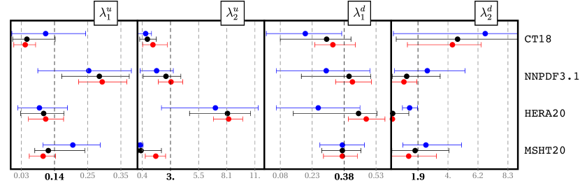
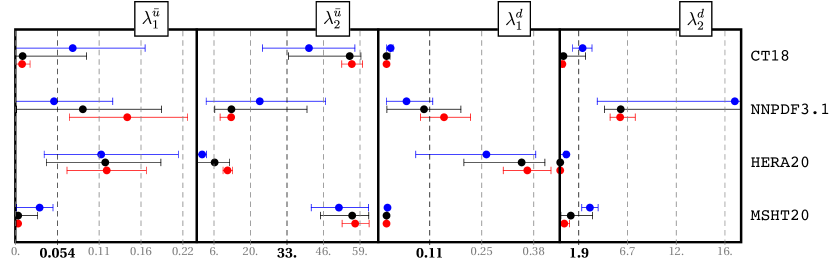
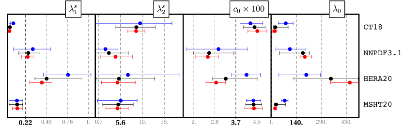
Figure 6: Comparison of the parameter values. Black is the final result. Blue is the value from the fit of the PDF case. Red is the value from the fit of the EXP case.

Parameter	MSHT20	HERA20	NNPDF31	CT18
$\lambda_{1}^{u}$	$0.12_{-0.04}^{+0.12}$	$0.11_{-0.07}^{+0.07}$	$0.28_{-0.10}^{+0.12}$	$0.05_{-0.05}^{+0.09}$
$\lambda_{2}^{u}$	$0.32_{-0.22}^{+1.84}$	$8.15_{-3.51}^{+2.09}$	$2.58_{-2.05}^{+1.37}$	$0.9_{-0.71}^{+0.84}$
$\lambda_{1}^{d}$	$0.37_{-0.10}^{+0.09}$	$0.44_{-0.31}^{+0.09}$	$0.40_{-0.22}^{+0.10}$	$0.29_{-0.22}^{+0.11}$
$\lambda_{2}^{d}$	$1.7_{-1.6}^{+2.4}$	$0.11_{-0.11}^{+1.14}$	$1.1_{-1.0}^{+2.4}$	$4.7_{-4.4}^{+5.0}$
$\lambda_{1}^{\bar{u}}\times 100$	$0.37_{-0.27}^{+2.51}$	$11.6_{-7.6}^{+7.1}$	$8.8_{-8.6}^{+10.1}$	$0.94_{-0.85}^{+8.14}$
$\lambda_{2}^{\bar{u}}$	$56._{-12.}^{+6.}$	$6.5_{-6.4}^{+5.5}$	$13._{-6.}^{+28.}$	$56._{-22.}^{+4.}$
$\lambda_{1}^{\bar{d}}\times 100$	$0.12_{-0.02}^{+0.18}$	$35._{-15.}^{+6.}$	$9.8_{-9.5}^{+9.4}$	$0.12_{-0.02}^{+0.86}$
$\lambda_{2}^{\bar{d}}$	$1.1_{-1.0}^{+2.4}$	$0.05_{-0.05}^{+0.09}$	$6.1_{-1.6}^{+16.7}$	$0.37_{-0.26}^{+2.20}$
$\lambda_{1}^{s}$	$0.11_{-0.10}^{+0.07}$	$0.49_{-0.15}^{+0.45}$	$0.25_{-0.12}^{+0.15}$	$0.012_{-0.011}^{+0.006}$
$\lambda_{2}^{s}$	$5.1_{-3.4}^{+3.3}$	$5.2_{-5.0}^{+7.7}$	$3.0_{-3.0}^{+4.3}$	$9.1_{-4.5}^{+4.2}$
$\lambda_{0}$	$29._{-10.}^{+53.}$	$339._{-212.}^{+156.}$	$181._{-133.}^{+39.}$	$24_{-11.}^{+73.}$
$c_{0}\times 100$	$4.36_{-0.31}^{+0.31}$	$3.27_{-0.52}^{+1.23}$	$2.61_{-0.61}^{+0.97}$	$4.39_{-0.44}^{+0.41}$

Table 5: The values of the NP parameters obtained in the fit.

The fits in refs. Bertone:2019nxa ; Scimemi:2019cmh ; Bacchetta:2019sam ; Vladimirov:2019bfa have found deficits in the predicted cross sections compared to measurements, with the deficits being small in the case of high-energy measurements (typically, $1$-$4$%) but more significant for low-energy measurements (typically, $30$-$40$%). In most cases, the discrepancy in the normalization is compensated by the correlated uncertainty of the experiment (e.g., E288 measurements have 25% uncertainty due to the beam luminosity), and thus does not significantly increase the value of $\chi^{2}$. Each PDF set requires its own normalization factor, e.g. for the central rapidity $Z$-boson production measured at ATLAS 8 TeV, the deficits are {3.6, 1.4, 2.1, 6.4}% for {MSHT20, HERA20, NNPDF3.1, CT18} cases. Another example is E288 at 200 GeV with {30, 49, 40, 39}%, correspondingly.

The actual shapes of the extracted TMDPDF are summarized in figs. 7, 8 and 9. We plot the “optimal” Scimemi:2019cmh ; Vladimirov:2019bfa TMD distribution, that is, the distribution defined according to the $\zeta$-prescription Scimemi:2017etj ; Scimemi:2018xaf as the reference, scaleless TMD distribution. Fig. 7 provides the overall picture as a function of $b$ and $x$. A more detailed view is offered by the slice in $b$ in fig. 8 and the slice in $x$ in fig. 9, showing the TMDPDF for each PDF set divided by the averaged central value of all PDF cases. The size of the uncertainty varies strongly from the low-$b$ region, where we have a good knowledge of the perturbative expansion, to the non-perturbative high-$b$ region (fig. 8). For $b\geq 2$ GeV^-1 the relative uncertainty on the TMD distributions is not less than 60-80$\%$. For comparison, figs. 8 and 9 also show the uncertainty band obtained in the fit Scimemi:2019cmh , labelled SV19. One of the main outcomes of the present work is that, compared to previous DY and SIDIS fits such as Scimemi:2019cmh , the TMD uncertainty obtained in this paper is about 4-5 times larger, as a result of the improved analysis framework taking into account the propagation of collinear PDF uncertainties to the TMD extraction and the flavor dependence of the TMD profile. Furthermore, note that the present extraction has a non-zero uncertainty band also at $b=0$, which was instead forbidden by construction in all previous studies.

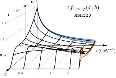
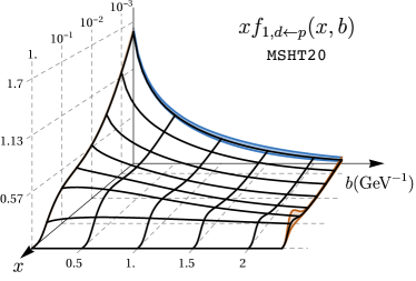
Figure 7: The optimal TMDPDF as a function of $(x,b)$ for $u$ and $d$ quarks with the MSHT20 PDF-input. The uncertainty is demonstrated at boundaries.

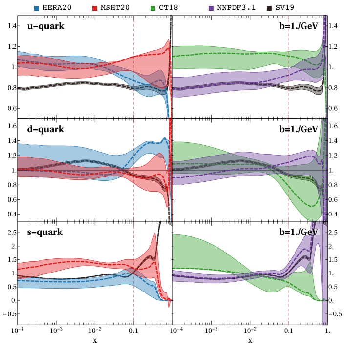
Figure 8: Comparison of uncertainty band for unpolarized TMDPDFs extracted with different PDFs. Here, the slice of optimal TMDPDF at $b=1$GeV^-1 is shown as the function of $x$. For convenience of presentation the plot is weighted with the central TMDPDF value averaged between different PDF cases. The red line indicates the position of slice demonstrated in fig.9.

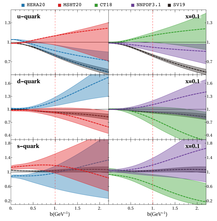
Figure 9: Comparison of the uncertainty band for unpolarized TMDPDFs extracted with different PDFs. Here, the slice of optimal TMDPDF at $x=0.1$ is shown as a function of $b$. For convenience of presentation the plot is weighted with the central TMDPDF value averaged between different PDF cases. The red line indicates the position of slice demonstrated in fig. 8.

The results presented in this section indicate that, compared to previous DY and SIDIS fits, the approach of the present paper leads to a more reliable estimate of the TMD uncertainties, to a reduced spread in the $\chi^{2}$ distribution for each PDF set, and to a better agreement between different PDF sets. Nevertheless, we see from figs. 8 and 9 that the TMDPDFs extracted with different PDFs still display significant differences. A similar remark applies to the CS kernel: results for the CS kernel extracted with different PDFs are shown in fig. 10.

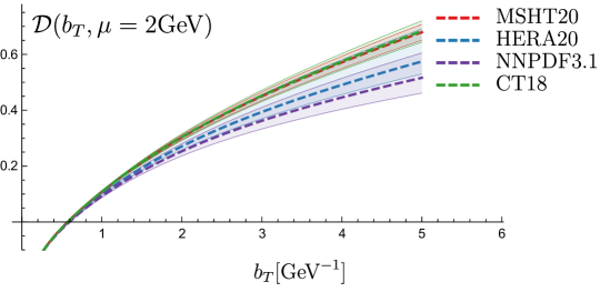
Figure 10: The CS-kernel as a function of $b$ extracted with different PDF inputs.

To further investigate the variation of TMDPDFs with the PDF set, we turn to Mellin moments of the TMDPDFs. We consider the following quantities

$$f^{(n)}_{f}(b)=\int_{x_{\text{min}}}^{1}dx\,x^{n-1}f_{1,f\leftarrow h}(x,b),$$ (21)

where we set $x_{\text{min}}=10^{-5}$. One may expect that the dependence on the collinear PDF is reduced, for $n=1$ and $n=2$, due to momentum sum rules fulfilled by each PDF set. Note however that $f_{\text{NP}}$ in eq. (7) contains a (weak) dependence on $x$. At any rate, the investigation of moments is significant because ratios for different flavours can be measured independently using lattice methods, see e.g. refs. Musch:2011er ; Schlemmer:2021aij . The ratios of the first moments for the light quarks with respect to the $u$-quark are shown in fig. 11. We see that, with respect to point-to-point comparisons, they display a better global agreement. A similar behaviour appears for the ratios of second and third moments. The corresponding plots are given in the supplementary material.

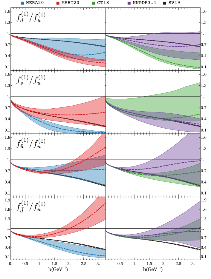
Figure 11: The ratio of the first Mellin moments of unpolarized TMDPDF (21) as a function of $b$ for different PDF cases.

We conclude this subsection by noting that the results for unpolarized TMD distributions presented above will also be important for the phenomenology of spin-dependent TMD distributions, where the unpolarized cross-section serves as the normalization for the measurements of polarization asymmetries and angular distributions. For example, the uncertainty band from the fit Scimemi:2019cmh resulted into 10-15% of the total uncertainty band for the Sivers function Bury:2020vhj . With the results of the present paper one can, on one hand, expect an extra $\sim 50\%$ uncertainty due to the inclusion of the PDF uncertainty. On the other hand, one can also expect a better agreement with experiments, due to a proper flavor dependence in the unpolarized sector.

5.3 Predictions for $W$-boson production

	CDF Abe:1991rk	D0 Abbott:1998jy	ATLAS Aad:2011fp			CMS Khachatryan:2016nbe
			$e$-channel	$\mu$-channel	combined	$e$-channel	$\mu$-channel
Points	10	10	2	2	2	4	4
MSHT20	0.66	1.8	2.9	1.6	2.5	8.1	32.
HERA20	0.68	2.0	1.7	0.6	1.2	5.9	23.
NNPDF31	0.70	1.8	2.5	1.3	2.0	7.6	30.
CT18	0.71	1.9	1.7	0.7	1.2	7.1	26.

Table 6: $\chi^{2}/N$ for differential $W$ production using the current extraction of TMD and theoretical errors (including PDF error coming from 1000 replicas).

The flavor dependence of the TMD distributions could significantly impact the description of processes mediated by the $W$-boson Signori:2013mda ; Bacchetta:2018lna ; Signori:2016lvd . In this work we have demonstrated that flavor dependence is essential to improve the agreement between theory and data. Including $W$-boson production data in future studies of unpolarized TMDPDFs will thus be very important.

Since it significantly slows down the fitting procedure, we have not included $W$-boson production data in this study. Instead, we compare the prediction made with the present extraction to the one made in Gutierrez-Reyes:2020ouu . The computation is performed with the artemide code, appropriately adapted for the computation of the transverse-mass-differential cross-section as described in ref. Gutierrez-Reyes:2020ouu . The values of the $\chi^{2}$ for comparison with the data by Tevatron and LHC experiments Abbott:1998jy ; Abe:1991rk ; Khachatryan:2016nbe ; Aad:2011fp are presented in tab. 6. We find a small general improvement compared to ref. Gutierrez-Reyes:2020ouu , which is expected because most of $W$-boson production data belong to the resummation region.

We see that the $\chi^{2}$ values for the CMS measurement are large in comparison with the other data considered. This may be understood by noting that this measurement is integrated over the full range of the dilepton mass, and the integration range covers low-mass regions in which power corrections in $q_{T}/Q$ are non-negligible. As a result, the theory prediction deviates from the measurement starting from smaller values of $q_{T}$, producing larger $\chi^{2}$-values. This effect is partially canceled in the cross-section ratios $W^{-}/W^{+}$ and $Z/W$, which show a substantial agreement between theory and the CMS measurements. Additional plots on this are presented in the supplementary material.

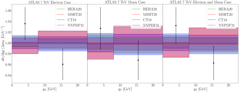
Figure 12: Comparison of the differential cross section for W-boson production measured by ATLAS at 7 TeV with the theory prediction using different PDFs and normalized to HERA20 case.

6 Conclusions

In this work we have performed the first quantitative study of the influence of PDF on fits to DY transverse momentum measurements based on TMD factorization. We have referred to this as the PDF bias issue, arising from the fact that an OPE is applied to the TMD operator and an ansatz is made for the TMD distribution in terms of collinear PDFs. We have highlighted the quantitative significance of this issue in unpolarized TMD fits. We have stressed that this is relevant also in polarized TMD analyses, for which unpolarized cross sections are used to normalize angular distributions and asymmetries.

We have carried out a Bayesian procedure to propagate PDF uncertainties to the extraction of TMD parton distributions. We have examined four PDF sets (MSHT20, NNPDF31, CT18, HERA20), representative of different NNLO PDF methodologies, and we have performed a TMD determination from DY data including for the first time both experimental and PDF uncertainties. We have found that the PDF uncertainties are larger than the DY experimental uncertainties for all values of $b$ (or $p_{T}$). As a result of the improved analysis framework, we have obtained reliable estimates of TMD uncertainties, with the size of TMD error bands being significantly increased with respect to previous TMD fits which do not perform the full PDF bias analysis.

We have included for the first time flavor dependence in the non-perturbative TMD distribution $f_{\text{NP}}^{f}$. Previous fits include flavor dependence in the collinear PDF only. We have found that flavor-dependent TMD profiles reduce the spread in $\chi^{2}$ distributions for each PDF set, improving the agreement between data and theory, and help obtain more consistent results among different PDF sets.

The results of this paper indicate that including collinear PDF uncertainties in TMD extractions and taking into account the flavor dependence of NP TMD distributions are both essential to obtain reliable TMD determinations from DY (and SIDIS) transverse momentum data. Future phenomenological studies, which incorporate these features with more powerful computational and statistical tools than those used here, are warranted.

Appendix A Appendix

In this appendix we provide a few more details and checks on the fits performed in sec. 5.

In fig. 2 we have presented our results for the distribution of $\chi^{2}$ values among the PDF and EXP replicas, and we have observed that the $\chi^{2}$ spread is much reduced with respect to previous fits in the literature, thanks to the flavor-dependent profile used in the present work for the NP TMD distributions $f_{\rm NP}^{f}$. Here we illustrate the role of the flavor dependence explicitly by reporting the result for the $\chi^{2}$ distribution which we obtain by repeating the calculation of fig. 2 but replacing the flavor-dependent $f_{\rm NP}^{f}$ model of eq. (7) with the flavor-independent model of ref. Scimemi:2019cmh . The result is shown in fig. 13 for the case of the NNPDF3.1 PDF set Ball:2017nwa .

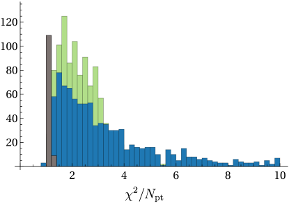
Figure 13: The same as fig. 2 in the case of a flavor independent $f_{\text{NP}}$ with the PDF set NNPDF3.1. The green histogram is obtained fitting $f_{\text{NP}}$ for each replica and the blue one is obtained keeping $f_{\text{NP}}$ fixed as from the fit of central replica. The grey histogram is the EXP error (see definition in sec.4.3).

The result in fig. 13 is to be compared with the third panel in fig. 2. We see that, in contrast to the $\chi^{2}$ distribution found in fig. 2, the distribution of $\chi^{2}$-values over PDF replicas in fig. 13 shows an unsatisfactorily broad shape, with about $64\%$ of the replicas having $\chi^{2}/N_{\text{pt}}>2$. We have checked that the unsatisfactory $\chi^{2}$-values for the subset of replicas are not due to a single problematic measurement but rather they are common to all data.

We have also checked that the issues described above are not specific to the NNPDF3.1 PDF set Ball:2017nwa . We performed similar tests using HERA20 Abramowicz:2015mha ($\chi^{2}_{0}/N_{\text{pt}}=0.97$), MMHT14 Harland-Lang:2014zoa ($\chi^{2}_{0}/N_{\text{pt}}=1.34$), CT14 Dulat:2015mca ($\chi^{2}_{0}/N_{\text{pt}}=1.59$), PDF4LHC15 Butterworth:2015oua ($\chi^{2}_{0}/N_{\text{pt}}=1.53$), MSHT20 Bailey:2020ooq ($\chi^{2}_{0}/N_{\text{pt}}=1.25$), CT18 Hou:2019efy ($\chi^{2}_{0}/N_{\text{pt}}=1.26$), and CJ15nlo Accardi:2016qay ($\chi^{2}_{0}/N_{\text{pt}}=1.82$), where $\chi^{2}_{0}$ is the $\chi^{2}$-value for the central PDF replica. All these PDF sets are characterized by the same issues as NNPDF3.1. This confirms that the essential element at the origin of the difference between the $\chi^{2}$ distributions in fig. 2 and fig. 13 is the flavor dependence of the NP TMD distributions $f_{\rm NP}^{f}$.

Figure 14: Examples of prediction using different PDF replicas at the same $f_{\text{NP}}$.

We next discuss the effect of different PDF replicas on the shape of the predictions for the transverse momentum distribution. One might wonder whether the change in PDF replicas results into an effect primarily on the normalization but not on the $q_{T}$ shape of the predictions. In fig. 14 we illustrate that this is not the case. That is, fig. 14 indicates that the large spread in the $\chi^{2}$ distribution observed above is due to different PDF replicas inducing different $q_{T}$-shapes of predictions. The variety of shapes is a consequence of the structure of the convolution within OPE, which correlates the $b$ and $x$ dependences.

References

- (1) K. Kovařík, P. M. Nadolsky and D. E. Soper, Hadronic structure in high-energy collisions, Rev. Mod. Phys. 92 (2020) 045003, [1905.06957].
- (2) R. Angeles-Martinez et al., Transverse Momentum Dependent (TMD) parton distribution functions: status and prospects, Acta Phys. Polon. B46 (2015) 2501–2534, [1507.05267].
- (3) S. M. Aybat and T. C. Rogers, TMD Parton Distribution and Fragmentation Functions with QCD Evolution, Phys. Rev. D83 (2011) 114042, [1101.5057].
- (4) I. Scimemi and A. Vladimirov, Non-perturbative structure of semi-inclusive deep-inelastic and Drell-Yan scattering at small transverse momentum, JHEP 06 (2020) 137, [1912.06532].
- (5) V. Bertone, I. Scimemi and A. Vladimirov, Extraction of unpolarized quark transverse momentum dependent parton distributions from Drell-Yan/Z-boson production, JHEP 06 (2019) 028, [1902.08474].
- (6) I. Scimemi and A. Vladimirov, Analysis of vector boson production within TMD factorization, Eur. Phys. J. C78 (2018) 89, [1706.01473].
- (7) A. Bacchetta, V. Bertone, C. Bissolotti, G. Bozzi, F. Delcarro, F. Piacenza et al., Transverse-momentum-dependent parton distributions up to N3LL from Drell-Yan data, JHEP 07 (2020) 117, [1912.07550].
- (8) A. Bacchetta, F. Delcarro, C. Pisano, M. Radici and A. Signori, Extraction of partonic transverse momentum distributions from semi-inclusive deep-inelastic scattering, Drell-Yan and Z-boson production, JHEP 06 (2017) 081, [1703.10157].
- (9) F. Hautmann and H. Jung, Transverse momentum dependent gluon density from DIS precision data, Nucl. Phys. B 883 (2014) 1, [1312.7875].
- (10) P. Kotko, K. Kutak, S. Sapeta, A. M. Stasto and M. Strikman, Estimating nonlinear effects in forward dijet production in ultra-peripheral heavy ion collisions at the LHC, Eur. Phys. J. C 77 (2017) 353, [1702.03063].
- (11) A. Bermudez Martinez, P. Connor, H. Jung, A. Lelek, R. Žlebčík, F. Hautmann et al., Collinear and TMD parton densities from fits to precision DIS measurements in the parton branching method, Phys. Rev. D 99 (2019) 074008, [1804.11152].
- (12) N. A. Abdulov et al., TMDlib2 and TMDplotter: a platform for 3D hadron structure studies, Eur. Phys. J. C 81 (2021) 752, [2103.09741].
- (13) F. Hautmann, H. Jung, M. Kramer, P. J. Mulders, E. R. Nocera, T. C. Rogers et al., TMDlib and TMDplotter: library and plotting tools for transverse-momentum-dependent parton distributions, Eur. Phys. J. C74 (2014) 3220, [1408.3015].
- (14) A. Apyan, D. Froidevaux et al., LHC Electroweak Working Group: W/Z transverse momentum benchmarking, CERN (2021) .
- (15) S. Camarda et al., DYTurbo: Fast predictions for Drell-Yan processes, Eur. Phys. J. C 80 (2020) 251, [1910.07049].
- (16) S. Camarda, L. Cieri and G. Ferrera, Drell–Yan lepton-pair production: qT resummation at N3LL accuracy and fiducial cross sections at N3LO, Phys. Rev. D 104 (2021) L111503, [2103.04974].
- (17) F. Coradeschi and T. Cridge, reSolve — A transverse momentum resummation tool, Comput. Phys. Commun. 238 (2019) 262, [1711.02083].
- (18) E. Accomando et al., Production of Z’-boson resonances with large width at the LHC, Phys. Lett. B 803 (2020) 135293, [1910.13759].
- (19) W. Bizon, X. Chen, A. Gehrmann-De Ridder, T. Gehrmann, N. Glover, A. Huss et al., Fiducial distributions in Higgs and Drell-Yan production at N3LL+NNLO, JHEP 12 (2018) 132, [1805.05916].
- (20) X. Chen, T. Gehrmann, E. W. N. Glover, A. Huss, P. F. Monni, E. Re et al., Third-Order Fiducial Predictions for Drell-Yan Production at the LHC, Phys. Rev. Lett. 128 (2022) 252001, [2203.01565].
- (21) M. A. Ebert, J. K. L. Michel, I. W. Stewart and F. J. Tackmann, Drell-Yan resummation of fiducial power corrections at N3LL, JHEP 04 (2021) 102, [2006.11382].
- (22) M. A. Ebert and F. J. Tackmann, Resummation of Transverse Momentum Distributions in Distribution Space, JHEP 02 (2017) 110, [1611.08610].
- (23) T. Becher and T. Neumann, Fiducial resummation of color-singlet processes at N3LL+NNLO, JHEP 03 (2021) 199, [2009.11437].
- (24) A. Vladimirov, Pion-induced Drell-Yan processes within TMD factorization, 1907.10356.
- (25) M. Bury, A. Prokudin and A. Vladimirov, Extraction of the Sivers Function from SIDIS, Drell-Yan, and Data at Next-to-Next-to-Next-to Leading Order, Phys. Rev. Lett. 126 (2021) 112002, [2012.05135].
- (26) M. G. Echevarria, Z.-B. Kang and J. Terry, Global analysis of the Sivers functions at NLO+NNLL in QCD, JHEP 01 (2021) 126, [2009.10710].
- (27) H1, ZEUS collaboration, H. Abramowicz et al., Combination of measurements of inclusive deep inelastic scattering cross sections and QCD analysis of HERA data, Eur. Phys. J. C75 (2015) 580, [1506.06042].
- (28) NNPDF collaboration, R. D. Ball et al., Parton distributions from high-precision collider data, Eur. Phys. J. C77 (2017) 663, [1706.00428].
- (29) T.-J. Hou et al., New CTEQ global analysis of quantum chromodynamics with high-precision data from the LHC, Phys. Rev. D 103 (2021) 014013, [1912.10053].
- (30) S. Bailey, T. Cridge, L. A. Harland-Lang, A. D. Martin and R. S. Thorne, Parton distributions from LHC, HERA, Tevatron and fixed target data: MSHT20 PDFs, Eur. Phys. J. C 81 (2021) 341, [2012.04684].
- (31) F. Hautmann, I. Scimemi and A. Vladimirov, Non-perturbative contributions to vector-boson transverse momentum spectra in hadronic collisions, Phys. Lett. B 806 (2020) 135478, [2002.12810].
- (32) J. Collins, Foundations of perturbative QCD. Cambridge University Press, 2013.
- (33) J. C. Collins, D. E. Soper and G. F. Sterman, Transverse Momentum Distribution in Drell-Yan Pair and W and Z Boson Production, Nucl. Phys. B250 (1985) 199–224.
- (34) T. Becher and M. Neubert, Drell-Yan Production at Small , Transverse Parton Distributions and the Collinear Anomaly, Eur. Phys. J. C71 (2011) 1665, [1007.4005].
- (35) M. G. Echevarria, A. Idilbi and I. Scimemi, Factorization Theorem For Drell-Yan At Low And Transverse Momentum Distributions On-The-Light-Cone, JHEP 07 (2012) 002, [1111.4996].
- (36) J.-Y. Chiu, A. Jain, D. Neill and I. Z. Rothstein, A Formalism for the Systematic Treatment of Rapidity Logarithms in Quantum Field Theory, JHEP 05 (2012) 084, [1202.0814].
- (37) I. Scimemi and A. Vladimirov, Systematic analysis of double-scale evolution, JHEP 08 (2018) 003, [1803.11089].
- (38) D. Gutierrez-Reyes, I. Scimemi, W. J. Waalewijn and L. Zoppi, Transverse momentum dependent distributions in and semi-inclusive deep-inelastic scattering using jets, JHEP 10 (2019) 031, [1904.04259].
- (39) D. Gutierrez-Reyes, S. Leal-Gomez and I. Scimemi, W-boson production in TMD factorization, Eur. Phys. J. C 81 (2021) 418, [2011.05351].
- (40) V. Moos and A. Vladimirov, Calculation of transverse momentum dependent distributions beyond the leading power, JHEP 12 (2020) 145, [2008.01744].
- (41) A. Vladimirov, V. Moos and I. Scimemi, Transverse momentum dependent operator expansion at next-to-leading power, 2109.09771.
- (42) J. C. Collins and D. E. Soper, Back-To-Back Jets in QCD, Nucl. Phys. B193 (1981) 381.
- (43) J. C. Collins and D. E. Soper, Back-To-Back Jets: Fourier Transform from B to K-Transverse, Nucl. Phys. B197 (1982) 446–476.
- (44) M. G. Echevarria, I. Scimemi and A. Vladimirov, Unpolarized Transverse Momentum Dependent Parton Distribution and Fragmentation Functions at next-to-next-to-leading order, JHEP 09 (2016) 004, [1604.07869].
- (45) M.-x. Luo, T.-Z. Yang, H. X. Zhu and Y. J. Zhu, Unpolarized quark and gluon TMD PDFs and FFs at N3LO, JHEP 06 (2021) 115, [2012.03256].
- (46) M.-x. Luo, T.-Z. Yang, H. X. Zhu and Y. J. Zhu, Quark Transverse Parton Distribution at the Next-to-Next-to-Next-to-Leading Order, Phys. Rev. Lett. 124 (2020) 092001, [1912.05778].
- (47) M. A. Ebert, B. Mistlberger and G. Vita, Transverse momentum dependent PDFs at N3LO, JHEP 09 (2020) 146, [2006.05329].
- (48) M. G. Echevarria, A. Idilbi, A. Schafer and I. Scimemi, Model-Independent Evolution of Transverse Momentum Dependent Distribution Functions (TMDs) at NNLL, Eur. Phys. J. C73 (2013) 2636, [1208.1281].
- (49) M. G. Echevarria, I. Scimemi and A. Vladimirov, Universal transverse momentum dependent soft function at NNLO, Phys. Rev. D93 (2016) 054004, [1511.05590].
- (50) A. A. Vladimirov, Soft-/rapidity- anomalous dimensions correspondence, Phys. Rev. Lett. 118 (2017) 062001, [1610.05791].
- (51) A. A. Vladimirov, Self-contained definition of Collins-Soper kernel, 2003.02288.
- (52) J. Collins and T. Rogers, Understanding the large-distance behavior of transverse-momentum-dependent parton densities and the Collins-Soper evolution kernel, Phys. Rev. D91 (2015) 074020, [1412.3820].
- (53) Lattice Parton collaboration, Q.-A. Zhang et al., Lattice QCD Calculations of Transverse-Momentum-Dependent Soft Function through Large-Momentum Effective Theory, Phys. Rev. Lett. 125 (2020) 192001, [2005.14572].
- (54) M. Schlemmer, A. Vladimirov, C. Zimmermann, M. Engelhardt and A. Schäfer, Determination of the Collins-Soper Kernel from Lattice QCD, JHEP 08 (2021) 004, [2103.16991].
- (55) P. Shanahan, M. Wagman and Y. Zhao, Lattice QCD calculation of the Collins-Soper kernel from quasi TMDPDFs, 2107.11930.
- (56) F. Hautmann, I. Scimemi and A. Vladimirov, Determination of the rapidity evolution kernel from Drell-Yan data at low transverse momenta, in 28th International Workshop on Deep Inelastic Scattering and Related Subjects, 9, 2021. 2109.12051.
- (57) A. V. Konychev and P. M. Nadolsky, Universality of the Collins-Soper-Sterman nonperturbative function in gauge boson production, Phys. Lett. B 633 (2006) 710–714, [hep-ph/0506225].
- (58) F. Landry, R. Brock, P. M. Nadolsky and C. P. Yuan, Tevatron Run-1 boson data and Collins-Soper-Sterman resummation formalism, Phys. Rev. D67 (2003) 073016, [hep-ph/0212159].
- (59) F. Landry, R. Brock, G. Ladinsky and C. P. Yuan, New fits for the nonperturbative parameters in the CSS resummation formalism, Phys. Rev. D63 (2001) 013004, [hep-ph/9905391].
- (60) F. Hautmann and D. E. Soper, Parton distribution function for quarks in an s-channel approach, Phys. Rev. D 75 (2007) 074020, [hep-ph/0702077].
- (61) F. Hautmann and D. E. Soper, Color transparency in deeply inelastic diffraction, Phys. Rev. D 63 (2001) 011501, [hep-ph/0008224].
- (62) F. Hautmann, Z. Kunszt and D. E. Soper, Hard scattering factorization and light cone Hamiltonian approach to diffractive processes, Nucl. Phys. B 563 (1999) 153–199, [hep-ph/9906284].
- (63) M. Guzzi, P. M. Nadolsky and B. Wang, Nonperturbative contributions to a resummed leptonic angular distribution in inclusive neutral vector boson production, Phys. Rev. D90 (2014) 014030, [1309.1393].
- (64) P. Schweitzer, T. Teckentrup and A. Metz, Intrinsic transverse parton momenta in deeply inelastic reactions, Phys. Rev. D81 (2010) 094019, [1003.2190].
- (65) P. Schweitzer, M. Strikman and C. Weiss, Intrinsic transverse momentum and parton correlations from dynamical chiral symmetry breaking, JHEP 01 (2013) 163, [1210.1267].
- (66) I. Scimemi and A. Vladimirov, Power corrections and renormalons in Transverse Momentum Distributions, JHEP 03 (2017) 002, [1609.06047].
-
(67)
“artemide web-page, https://teorica.fis.ucm.es/artemide/.
artemide repository, https://github.com/VladimirovAlexey/artemide-public. The W-boson case is in https://github.com/SergioLealGomezTMD/artemide-development.” - (68) A. Buckley, J. Ferrando, S. Lloyd, K. Noerdstrom, B. Page, M. Ruefenacht et al., LHAPDF6: parton density access in the LHC precision era, Eur. Phys. J. C75 (2015) 132, [1412.7420].
- (69) H. Dembinski and P. O. et al., scikit-hep/iminuit, .
- (70) A. Bermudez Martinez et al., Production of Z-bosons in the parton branching method, Phys. Rev. D 100 (2019) 074027, [1906.00919].
- (71) A. Bermudez Martinez et al., The transverse momentum spectrum of low mass Drell–Yan production at next-to-leading order in the parton branching method, Eur. Phys. J. C 80 (2020) 598, [2001.06488].
- (72) J. C. Collins and F. Hautmann, Soft gluons and gauge invariant subtractions in NLO parton shower Monte Carlo event generators, JHEP 03 (2001) 016, [hep-ph/0009286].
- (73) A. S. Ito et al., Measurement of the Continuum of Dimuons Produced in High-Energy Proton - Nucleus Collisions, Phys. Rev. D23 (1981) 604–633.
- (74) G. Moreno et al., Dimuon production in proton - copper collisions at = 38.8-GeV, Phys. Rev. D43 (1991) 2815–2836.
- (75) E772 collaboration, P. L. McGaughey et al., Cross-sections for the production of high mass muon pairs from 800-GeV proton bombardment of H-2, Phys. Rev. D50 (1994) 3038–3045.
- (76) PHENIX collaboration, C. Aidala et al., Measurements of pairs from open heavy flavor and Drell-Yan in collisions at GeV, Submitted to: Phys. Rev. D (2018) , [1805.02448].
- (77) CDF collaboration, T. Affolder et al., The transverse momentum and total cross section of pairs in the boson region from collisions at TeV, Phys. Rev. Lett. 84 (2000) 845–850, [hep-ex/0001021].
- (78) CDF collaboration, T. Aaltonen et al., Transverse momentum cross section of pairs in the -boson region from collisions at TeV, Phys. Rev. D86 (2012) 052010, [1207.7138].
- (79) D0 collaboration, B. Abbott et al., Measurement of the inclusive differential cross section for bosons as a function of transverse momentum in collisions at TeV, Phys. Rev. D61 (2000) 032004, [hep-ex/9907009].
- (80) D0 collaboration, V. M. Abazov et al., Measurement of the shape of the boson transverse momentum distribution in events produced at =1.96-TeV, Phys. Rev. Lett. 100 (2008) 102002, [0712.0803].
- (81) D0 collaboration, V. M. Abazov et al., Measurement of the normalized transverse momentum distribution in collisions at TeV, Phys. Lett. B693 (2010) 522–530, [1006.0618].
- (82) ATLAS collaboration, G. Aad et al., Measurement of the boson transverse momentum distribution in collisions at = 7 TeV with the ATLAS detector, JHEP 09 (2014) 145, [1406.3660].
- (83) ATLAS collaboration, G. Aad et al., Measurement of the transverse momentum and distributions of Drell-Yan lepton pairs in proton-proton collisions at TeV with the ATLAS detector, Eur. Phys. J. C76 (2016) 291, [1512.02192].
- (84) CMS collaboration, S. Chatrchyan et al., Measurement of the Rapidity and Transverse Momentum Distributions of Bosons in Collisions at TeV, Phys. Rev. D85 (2012) 032002, [1110.4973].
- (85) CMS collaboration, V. Khachatryan et al., Measurement of the transverse momentum spectra of weak vector bosons produced in proton-proton collisions at TeV, JHEP 02 (2017) 096, [1606.05864].
- (86) CMS collaboration, A. M. Sirunyan et al., Measurements of differential Z boson production cross sections in proton-proton collisions at = 13 TeV, JHEP 12 (2019) 061, [1909.04133].
- (87) LHCb collaboration, R. Aaij et al., Measurement of the forward boson production cross-section in collisions at TeV, JHEP 08 (2015) 039, [1505.07024].
- (88) LHCb collaboration, R. Aaij et al., Measurement of forward W and Z boson production in collisions at TeV, JHEP 01 (2016) 155, [1511.08039].
- (89) LHCb collaboration, R. Aaij et al., Measurement of the forward Z boson production cross-section in pp collisions at TeV, JHEP 09 (2016) 136, [1607.06495].
- (90) NNPDF collaboration, R. D. Ball, L. Del Debbio, S. Forte, A. Guffanti, J. I. Latorre, A. Piccione et al., A Determination of parton distributions with faithful uncertainty estimation, Nucl. Phys. B809 (2009) 1–63, [0808.1231].
- (91) R. D. Ball et al., Parton Distribution Benchmarking with LHC Data, JHEP 04 (2013) 125, [1211.5142].
- (92) T.-J. Hou et al., Reconstruction of Monte Carlo replicas from Hessian parton distributions, JHEP 03 (2017) 099, [1607.06066].
- (93) A. Bacchetta, V. Bertone, C. Bissolotti, G. Bozzi, M. Cerutti, F. Piacenza et al., Unpolarized Transverse Momentum Distributions from a global fit of Drell-Yan and Semi-Inclusive Deep-Inelastic Scattering data, 2206.07598.
- (94) B. U. Musch, P. Hagler, M. Engelhardt, J. W. Negele and A. Schafer, Sivers and Boer-Mulders observables from lattice QCD, Phys. Rev. D 85 (2012) 094510, [1111.4249].
- (95) CDF collaboration, F. Abe et al., Measurement of the W P(T) distribution in collisions at TeV, Phys. Rev. Lett. 66 (1991) 2951–2955.
- (96) D0 collaboration, B. Abbott et al., Measurement of the shape of the transverse momentum distribution of bosons produced in collisions at TeV, Phys. Rev. Lett. 80 (1998) 5498–5503, [hep-ex/9803003].
- (97) ATLAS collaboration, G. Aad et al., Measurement of the Transverse Momentum Distribution of Bosons in Collisions at TeV with the ATLAS Detector, Phys. Rev. D 85 (2012) 012005, [1108.6308].
- (98) A. Signori, A. Bacchetta, M. Radici and G. Schnell, Investigations into the flavor dependence of partonic transverse momentum, JHEP 11 (2013) 194, [1309.3507].
- (99) A. Bacchetta, G. Bozzi, M. Radici, M. Ritzmann and A. Signori, Effect of Flavor-Dependent Partonic Transverse Momentum on the Determination of the Boson Mass in Hadronic Collisions, Phys. Lett. B 788 (2019) 542–545, [1807.02101].
- (100) A. Signori, Flavor and Evolution Effects in TMD Phenomenology: Manifestation of Hadron Structure in High-Energy Scattering Processes. PhD thesis, Vrije U., Amsterdam, 2016.
- (101) L. A. Harland-Lang, A. D. Martin, P. Motylinski and R. S. Thorne, Parton distributions in the LHC era: MMHT 2014 PDFs, Eur. Phys. J. C75 (2015) 204, [1412.3989].
- (102) S. Dulat, T.-J. Hou, J. Gao, M. Guzzi, J. Huston, P. Nadolsky et al., New parton distribution functions from a global analysis of quantum chromodynamics, Phys. Rev. D93 (2016) 033006, [1506.07443].
- (103) J. Butterworth et al., PDF4LHC recommendations for LHC Run II, J. Phys. G43 (2016) 023001, [1510.03865].
- (104) A. Accardi, L. T. Brady, W. Melnitchouk, J. F. Owens and N. Sato, Constraints on large- parton distributions from new weak boson production and deep-inelastic scattering data, Phys. Rev. D 93 (2016) 114017, [1602.03154].