Lifelong Dynamic Optimization for Self-Adaptive Systems: Fact or Fiction?

Abstract

When faced with changing environment, highly-configurable software systems need to dynamically search for promising adaptation plan that keeps the best possible performance, e.g., higher throughput or smaller latency — a typical planning problem for self-adaptive systems (SASs). However, given the rugged and complex search landscape with multiple local optima, such a SAS planning is challenging especially in dynamic environments. In this paper, we propose LiDOS, a lifelong dynamic optimization framework for SAS planning. What makes LiDOS unique is that to handle the “dynamic”, we formulate the SAS planning as a multi-modal optimization problem, aiming to preserve the useful information for better dealing with the local optima issue under dynamic environment changes. This differs from existing planners in that the “dynamic” is not explicitly handled during the search process in planning. As such, the search and planning in LiDOS run continuously over the lifetime of SAS, terminating only when it is taken offline or the search space has been covered under an environment.

Experimental results on three real-world SASs show that the concept of explicitly handling dynamic as part of the search in the SAS planning is effective, as LiDOS outperforms its stationary counterpart overall with up to $10\times$ improvement. It also achieves better results in general over state-of-the-art planners and with $1.4\times$ to $10\times$ speedup on generating promising adaptation plans.

I Introduction

Many software systems are highly-configurable, thereby making them flexible to different needs. When operating under dynamic and uncertain environment, those systems are capable of changing their own configuration at runtime with an aim to achieve the best of their performance objective, e.g., higher throughput or smaller latency [1, 2] — a typical type of self-adaptive systems (SASs) that we consider in this work. For example, Apache Storm, a stream processing framework, can change some adaptation options (e.g., num_counters and num_splitters) at runtime to react to the changing batch of the jobs with different types and workloads [3, 4].

In SAS, a crucial problem is planning [5, 6, 7, 8], i.e., what is the next best adaptation plan to take under time-varying environments? From the literature, a promising research direction for tackling this challenges is relying on the paradigm of Search-Based Software Engineering (SBSE), where a search algorithm is used to continuously find the optimal plan for SASs [9, 10, 11, 12, 13, 14, 15, 16]. Indeed, search and optimization is at the fundamental part of the planning, and it is complementary to the other approaches, such as control theoretical [17, 18, 19] and learning-based [20, 21, 22, 23, 24, 25].

Figure 1: A projected landscape of the Throughput with respect to adaptation options Splitters and Counters for Storm under the RollingCount environment.  and  denote the global and local optimum, respectively.

Yet, apart from the exponentially growing search space and non-linear interaction between the options, what makes the planning particularly difficult is the presence of high sparsity in highly-configurable systems. That is, as shown by Nair et al. [3] and Jamshidi et al. [4], the neighboring adaptation plans can also have drastically different performance given an environment, leading to a highly complex search landscape. For example, we see a rather rugged landscape from Figure 1 on the case of Storm under the WordCount environment, where there are many local optima — the sub-optimal adaptation plans for which all the neighboring plans have worse performance — that can easily trap the planner. As a result, the produced plans may be far away from the global optimum, especially considering that the planner needs to produce a plan efficiently with little overhead. As we will show in Section III-A, the landscape can differ following dynamic environmental changes, which further complicates the SAS planning.

In this paper, we tackle the above challenge by proposing LiDOS, a framework that implements the concept of lifelong and truly dynamic optimization for SAS planning. By designing a mechanism that takes the characteristics of SAS planning into account, the “dynamic” we consider refers to the case that the changes are explicitly captured as the search in the planner proceeds, which is the exact definition of dynamic optimization coined by Nguyen et al. [26], hence the useful information for planning after the change can be preserved to better overcome local optima. As such, the search and optimization in LiDOS runs continuously, terminating only when the SAS is taken offline or all search space has been covered under an environment — the true lifelong optimization. In this way, we hope to make the lifelong dynamic optimization more factual for SASs. This differs from previous SBSE work for SAS planning where dynamic optimization is more “fictional”, such that the planner is pseudo-dynamic because, although it runs continuously, the true “dynamic” is not explicitly considered in the search, but a vanilla search algorithm is directly adopted and hoping that the changes will eventually be coped with via the re-evaluated fitness [12, 13, 14, 15]; it can also be distinguished from the stationary planners, in which the planning is restarted from scratch upon an environmental change or based on a fixed frequency [9, 10, 11]. Both the pseudo-dynamic and stationary planners are not ideal given the rugged landscape and the need of timely planning for SAS.

The key novelty of this work is that we formulate the lifelong dynamic optimization for SAS as a multi-modal optimization problem. This was inspired by our observation that, for highly-configurable systems, the global optimum of performance in an environment is likely to be (or very close to) a local optimum in the other. Our aim is to continuously preserve as many local optima as possible without losing the tendency towards achieving the global optimum, hence the planning can better deal with the complex landscape even under environmental changes. The core of LiDOS for tackling the multi-modal optimization problem is a refined MMO — the meta multi-objectivization model proposed by Chen and Li at FSE’21 [27], because (1) it is simple; (2) it fits the needs of a multi-modal optimization problem; and (3) it has been shown to be promising in mitigating local optima traps for highly-configurable systems. In a nutshell, our contributions are:

1. We formulate the lifelong dynamic optimization for SAS planning as a multi-modal optimization problem motivated by characteristics of the highly-configurable systems.

2. To solve the multi-modal optimization problem, we refine the MMO with a new auxiliary objective that can be easily measured, and no normalization is required, thereby eliminating the need of tuning the weight, which has been shown as a highly sensitive parameter in MMO [27].

3. We design an architecture that uses a hierarchical feedback loop to realize the concept of lifelong dynamic optimization for SASs, where the search in planning runs continuously and the dynamic changes that occur during the run are explicitly handled.

4. Through experiments on three real-world SASs of different performance objectives, scales, complexity, and under six environments, we evaluate LiDOS against its stationary variant (for ablation analysis), as well as state-of-the-art pseudo-dynamic [12, 15] and stationary planners [9].

The results are encouraging: we observe that when comparing with its stationary variant, LiDOS produces considerably better adaptation plans in general (with $p<0.05$ and high effect size) and up to $10\times$ improvement. LiDOS also performs significantly better overall than the state-of-the-art planners with greater efficiency: it shows $1.4\times$ to $5\times$ speedup of planning over the pseudo-dynamic planners and $2.5\times$ to $10\times$ speedup on the stationary one. This proves that lifelong (truly) dynamic optimization for SAS planning is more of a fact than fiction.

To promote open science, the code and data in this work can be accessed at: https://doi.org/10.5281/zenodo.5586103.

In what follows, Section II introduces the background. Section III elaborates the motivation and design of our LiDOS framework. Section IV presents our experiment methodology, followed by a discussion of the results in Section V. The threats to validity are discussed in Section VI. Sections VII and VIII analyze the related work and conclude the paper, respectively.

II Preliminaries

Here, we describe the necessary background and context.

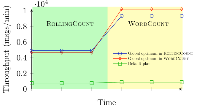
Figure 2: Changing throughput on Storm from the RollingCount to WordCount environment (highlighted areas), each of which has different batches of jobs, types and workloads.

II-A Self-Adaptation for Configurable Systems

While the purpose of self-adaptation can vary, in this work, we focus on improving the performance of highly-configurable systems such as smaller latency and higher throughput. We model this type of SAS with $n$ adaptation options such that the $i$th option is denoted as $x_{i}$, which can be either a binary or integer variable. The search space of all adaptation plans, $\mathbfcal{X}$, is the Cartesian product of the possible values for all the $x_{i}$. Formally, the ultimate goal is to achieve the following for every monitoring timestep despite the environment changes:

$$\operatorname*{argmin}~{}f(\boldsymbol{x}),~{}~{}\boldsymbol{x}\in\mathbfcal{X}$$ (1)

where $\boldsymbol{x}=(x_{1},x_{2},...,x_{n})$. However, recall the landscape shown in Figure 1, the planner may be easily trapped at some of the undesired local optima, making the problem non-trivial to address. The need for planning with less overhead (due to large search space and/or expensive measurements) makes it even more challenging. An additional complication with SAS is that, as the environment change, the search landscape can also change, which we will discuss in Section III-A.

As a concrete example in Figure 2, Storm can handle data streaming process under various environments on the incoming batch of jobs, e.g., RollingCount and WordCount. We see that (1) although the default plan leads to different results across the environments, it performs fairly poor overall — compared with the global optimum, it is $6.4\times$ worse on RollingCount and $11.5\times$ worse on WordCount; (2) the global optimum can differ for different environments. All above motivate the need of self-adaptation for Storm, where the aim is to achieve the best possible throughput by searching the right adaptation plan, e.g., settings for num_counters and num_splitters, over changing environments.

II-B Dynamic Optimization

Given the increasingly growing field of SBSE, search algorithms have been widely applied to various software engineering tasks [28]. Indeed, any search algorithm is dynamic in nature, i.e., they dynamically determine what direction to explore or which solutions to keep depending on the fitness during the search. However, the active field of dynamic optimization means a different concept. According to Nguyen et al. [26], dynamic optimization refers to the case where the “algorithm needs to take into account changes during the optimization process as time goes by.” The changes here refer to the change in search landscape, including fitness function, global/local optimum and the optimization objectives, etc.

Despite there being a good match between the definition of dynamic optimization and the requirement for SASs, truly dynamic optimization has rarely been explored. Often, the planner with a search algorithm may either be stationary (restart the search whenever upon an environmental change or upon a fixed frequency) [9, 10, 11]; or pseudo-dynamic [12, 13, 14, 15], i.e., there is no mechanism to handle the potential impact on the search landscape when environmental change occurs, but hoping the nature of the search algorithm can eventually adapt to it using the re-evaluated fitness. Both of the two ways can waste valuable information that would benefit the search after the change, especially considering the highly rugged landscape for SASs from Figure 1. However, the difficulties of truly dynamic optimization for SASs are:

1. What information from the planning before the environmental change is useful for planning thereafter?

2. How to identify and preserve such information?

This paper tackles the above difficulties in the next section.

III Designing LiDOS

In this section, we present the motivations and technical designs behind LiDOS.

III-A Key Characteristics of SAS Changes

A clear characteristic for SAS planning from Figure 1 is:

• Characteristic 1: Highly-configurable systems often come with a multi-modal landscape, i.e., there can be many local optima, making the planner to be easily trapped at them. This is consistent with what has been reported from prior studies on highly-configurable systems [3, 4].

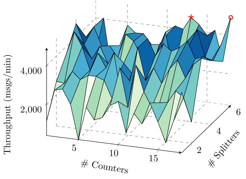
(a) Storm under RollingCount

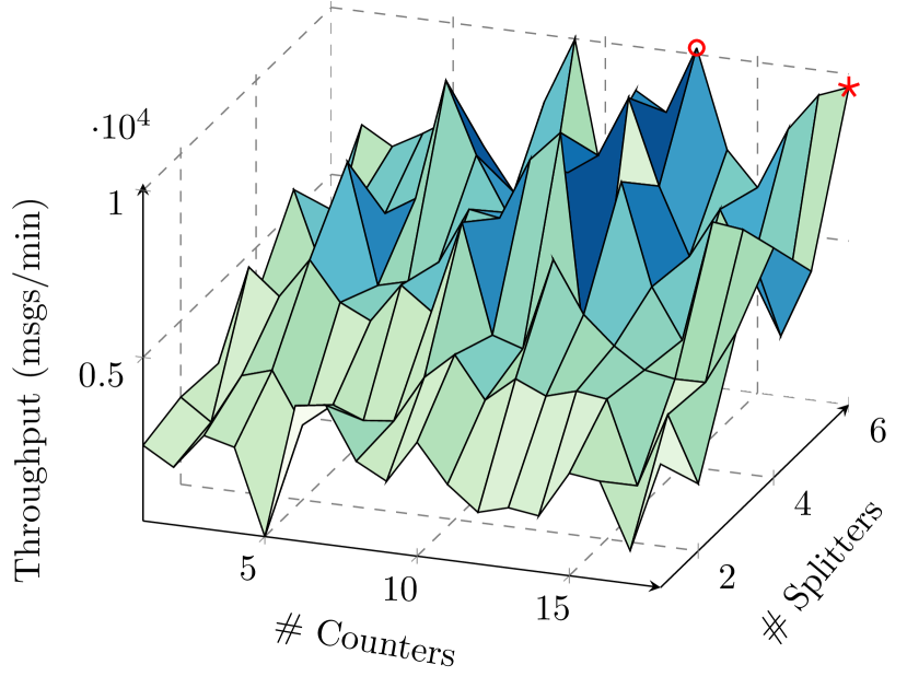
(b) Storm under WordCount

Figure 3: A projected landscape of the Throughput with respect to adaptation options Splitters and Counters for Storm under the RollingCount and WordCount environment.  denotes the global optimum in an environment and  denotes a local optimum for the same environment, which is also the global optimum in the other environment.

By investigating the performance under different environments of the SAS studied in this work using fitness landscape analysis [29, 30], we additionally observed some common patterns and found that (Figure 3 is an example of Storm):

• Characteristic 2: The search landscape does change across different environments, including the global optimum, but the overall multi-modal property is still preserved and there are shared local optima. This matches with the insight by Jamshidi et al. [25], which states that the performance values between diverse environments, although different, share similar distribution (an indicator of similar ruggedness/peakedness [29]), hence the model of the landscape can be linearly transferred.

• Characteristic 3: The global optimum in one environment is likely to become a local optimum (which is close to the new global optimum) under another environment. This has also been hinted by evidence from the literature [25].

The above suggests that the change of environments for SAS can indeed impact the search landscape, but there is certain information on the multi-modality that can be shared before and after the environmental change. This means that truly dynamic optimization that improves the plan continuously is vital for SAS, yet we need a specific mechanism to handle the dynamic changes as the search proceeds and achieve two goals:

• Goal 1: preserving as many local optima as possible, since they can provide useful information upon environmental change (Characteristic 2 and 3).

• Goal 2: but doing so without losing the tendency towards finding the global optimum (Characteristic 1).

III-B Multi-objectivization with Multi-modality

Goal 1 motivates us to formulate the SAS planning as a multi-modal optimization problem [31], for which there exist quite a few search algorithms. However, those algorithms prioritize exploring more local optima while may negatively affecting Goal 2, hence they are ill-suited to our problem. As a result, in LiDOS, we refine the meta multi-objectivization (MMO) model proposed by Chen and Li at FSE’21 [27] for achieving Goal 1 and Goal 2 simultaneously.

In a nutshell, MMO is a recently proposed way of optimization for configurable and self-adaptive systems. The idea is to “multi-objectivize” the problem using an additional auxiliary objective. Unlike existing work that focuses on the algorithm level, MMO works at the more generic level of optimization model which is compatible with different multi-objective search algorithms, e.g., NSGA-II [32]. Formally, MMO is defined as:

$$\begin{split}\text{minimize}\begin{cases}g_{1}(\boldsymbol{x})=f_{t}(\boldsymbol{x})+w\times f_{a}(\boldsymbol{x})\\ g_{2}(\boldsymbol{x})=f_{t}(\boldsymbol{x})-w\times f_{a}(\boldsymbol{x})\\ \end{cases}\end{split}$$ (2)

whereby $g_{1}(\boldsymbol{x})$ and $g_{2}(\boldsymbol{x})$ are the newly transformed objectives to be optimized; $f_{t}(\boldsymbol{x})$ is the target performance objective that is of concerned, e.g., throughput; $f_{a}(\boldsymbol{x})$ is the auxiliary objective of an additional performance attribute such that, under the given context, no stakeholders care about its value, e.g., CPU load. $w$ is a weight parameter that balances the contributions. While MMO was not originally designed for multi-modal problem but for more efficiently mitigating the issues of local optima, the uniqueness lies in that it simultaneously possesses the following properties in the transformed space:

1. Because of the Pareto dominance relation on $g_{1}(\boldsymbol{x})$ and $g_{2}(\boldsymbol{x})$, MMO preserves adaptation plans that with very different values of $f_{a}(\boldsymbol{x})$ (despite being similar on $f_{t}(\boldsymbol{x})$) as they tend to be incomparable in the sense of Pareto dominance. This encourages the search to explore a wider range of the search space and hence more likely to find and preserve different local optima, i.e., fitting the multi-modal property in nature (thereby satisfying Goal 1).

2. The global optimum of the original $f_{t}(\boldsymbol{x})$ is still Pareto-optimal in the transformed space. In particular, if adaptation plan $\boldsymbol{x_{1}}$ has a better target performance objective than $\boldsymbol{x_{2}}$ (i.e., $f_{t}(\boldsymbol{x_{1}})<f_{t}(\boldsymbol{x_{2}})$), then whatever their auxiliary objective values are, $\boldsymbol{x_{2}}$ will not be better than $\boldsymbol{x_{1}}$ on both $g_{1}$ and $g_{2}$; in the best case for $\boldsymbol{x_{2}}$, they are nondominated to each other (hence suitable for Goal 2). Note that naively optimize the raw $f_{t}(\boldsymbol{x})$ and $f_{a}(\boldsymbol{x})$ (instead of $g_{1}(\boldsymbol{x})$ and $g_{2}(\boldsymbol{x})$) is harmful to Goal 2, as the search would be forced to optimize $f_{a}(\boldsymbol{x})$, which is of no interest to us.

In this regard, MMO is a perfect fit for our problem of lifelong dynamic optimization for SAS planning. We refer interested readers to the work of Chen and Li [27] for more detailed examples and proofs of the above.

However, we cannot directly apply MMO to our problem due primarily to two reasons:

1. The $f_{a}(\boldsymbol{x})$ in MMO was deigned to be an additional performance objective. This is, however, not ideal for SAS planning, as it may introduce extra measurement overhead that can be harmful for runtime adaptation.

2. More importantly, since $f_{t}(\boldsymbol{x})$ and $f_{a}(\boldsymbol{x})$ often come with rather different scales for SASs [9, 11], normalization is required. Chen and Li [27] has shown that under such a case, the $w$ can become a highly-sensitive parameter to tune before using MMO in the search. This is clearly difficult for SASs where pre-tuning is infeasible.

Thus in this work, we refine MMO by replacing the $f_{a}(\boldsymbol{x})$.

1

Input: Adaptation plan space $\mathcal{V}$; the Cyber-Twin of managed system $\mathcal{F}$; adaptation interval $k$

2

Declare: $s_{best}$ the best adaptation plan on $f_{t}(\boldsymbol{x})$

3 Randomly initialize a population of $n$ adaptation plan $\mathcal{P}$

4

5measure($\mathcal{P},\mathcal{F}$)

6 $t=t+n$

7 while The search space has not been covered in the current environment and the system still runs do

8      

9      $\mathcal{P^{\prime}}=\emptyset$

10      

11      while $\mathcal{P^{\prime}}<n$ do

12            

13            $\{s_{x},s_{y}\}\leftarrow$mating($\mathcal{P}$)

14            $\{o_{x},o_{y}\}\leftarrow$doCrossoverAndMutation($\mathcal{V},s_{x},s_{y}$)

15             /* in the same environment, only newly explored plans need to be measured; re-emerged ones can reuse the previously measured objectives. */

16             if $o_{x}$ is new in current environment then

17                   measure($o_{x},\mathcal{F}$)

18                   $t=t+1$

19                  

20            if $o_{y}$ is new in current environment then

21                   measure($o_{y},\mathcal{F}$)

22                   $t=t+1$

23                  

24            

25            $\mathcal{P^{\prime}}\leftarrow\mathcal{P^{\prime}}\bigcup\{o_{x},o_{y}\}$

26            

27      

28      $\mathcal{U^{\prime}}\leftarrow$$\mathcal{P}\bigcup\mathcal{P^{\prime}}$

29      

30      for $\forall s^{\prime}\in\mathcal{U^{\prime}}$ do

31             $\mathcal{N}\leftarrow$getCloestNeighboringPlans($s^{\prime}$,$\mathcal{U^{\prime}}$)

32            

33            $a\leftarrow$getMostDissimilarPlanOnTarget($s^{\prime}$,$\mathcal{N}$)

34            

35            $f_{a}(\boldsymbol{x})$ of $s^{\prime}\leftarrow f_{t}(\boldsymbol{x})$ of $a$

36            

37      

38      computeMMOModel($\mathcal{U^{\prime}}$)

39      

40      $\mathcal{U}\leftarrow$nondominatedSorting($\mathcal{U^{\prime}}$)

41       $\mathcal{P}\leftarrow$top $n$ adaptation plans from $\mathcal{U}$

42       $s^{\prime}_{best}\leftarrow$bestPlan($\mathcal{P}$)

43       if $s^{\prime}_{best}$ is better than $s_{best}$ then

44             $s_{best}\leftarrow s^{\prime}_{best}$

45            

46      

47      /* adapt the managed system with a better plan upon every $k$ new measurements. */

48       if $t\geq k$ and $s_{best}$ has not been sent then

49             $t=0$

50             sendForAdaptation($s_{best}$)

51      

52

Algorithm 1 Multi-objectivization Planner for SASs

III-C Refined MMO based Planning

Refining MMO by finding an appropriate replacement of the auxiliary objective $f_{a}(\boldsymbol{x})$ is non-trivial, as we need to ensure that (1) $f_{a}(\boldsymbol{x})$ is an easy-to-measure objective; and (2) it should be within the same scale as that of $f_{t}(\boldsymbol{x})$ (hence the $w$ can be removed by setting $w=1$) while (3) similarly performing adaptation plans on $f_{t}(\boldsymbol{x})$ can have very different values on $f_{a}(\boldsymbol{x})$, which is an important requirement for multi-objectivization with MMO as shown by Chen and Li [27].

Since MMO is often used with a population-based multi-objective search algorithm (we use NSGA-II in this work), to replace the $f_{a}(\boldsymbol{x})$ in MMO, we focus on using the neighboring adaptation plans in the current population (and generated offsprings) during the search. Algorithm 1 shows the pseudo-code for the refined MMO using NSGA-II as the underlying algorithm for SAS planning. As can be seen, to use MMO, the key is that selecting which adaptation plan to preserve will be done in the transformed space ($g_{1}(\boldsymbol{x})$ and $g_{2}(\boldsymbol{x})$) instead of the original space (line 22). Since it is impractical to influence the managed system during planning, the measurements of unique adaptation plans are conducted on a Cyber-Twin of the system to be managed (line 2, 11 and 14).

Specifically, at each iteration/generation, we compute the $f_{a}(\boldsymbol{x_{s}})$ for an adaptation plan $\boldsymbol{x_{s}}$ as the follows:

1. Find the adaptation plan(s) $\mathcal{N}=\{\boldsymbol{x_{1}},\boldsymbol{x_{2}},...,\boldsymbol{x_{k}}\}$ with the closest distance (in terms of the variable space $\boldsymbol{x}$) to $\boldsymbol{x_{s}}$ in the current population/offsprings. We use Euclidean distance as it offers good discriminative power (line 19).

2. Identify the $\boldsymbol{x_{a}}$ from $\mathcal{N}$ such that its $f_{t}(\boldsymbol{x_{a}})$ has the largest difference to $f_{t}(\boldsymbol{x_{s}})$, and then set $f_{a}(\boldsymbol{x_{s}})=f_{t}(\boldsymbol{x_{a}})$. In this way, we reduce the chance of having $f_{t}(\boldsymbol{x_{s}})=f_{a}(\boldsymbol{x_{s}})$, which essentially invalidates multi-objectivization (line 20-21).

Clearly, the new auxiliary objective $f_{a}(\boldsymbol{x})$ is easy-to-measure and it will have the same scale as $f_{t}(\boldsymbol{x})$. While the neighboring plans for SASs may behave similarly on the performance, Nair et al. [3] have shown that for highly-configurable systems, those neighboring plans can also lead to radically different results. The is because, for example, when two plans only differ on whether to turn on the cache option, the performance results can differ dramatically even though these plans exhibit very similar representation in the search algorithm. Similar observations have also been registered by the others [4]. As a result, our design also ensures that adaptation plans can have similarly-performing $f_{t}(\boldsymbol{x})$ but very different $f_{a}(\boldsymbol{x})$.

Since LiDOS is a lifelong dynamic optimization framework, the multi-objectivization planner terminates when all the search space in an environment has been explored, or otherwise, it runs throughout the lifetime of the SASs. An adaptation to the managed system is triggered every $k$ new measurements and when a better plan has been found (line 29-31). Here, $k$ serves as a parameter that determines the extent of convergence and tolerated overhead for the planning in LiDOS.

III-D Architecture

Figure 4 shows the architecture of LiDOS, which uses a hierarchical feedback loop. As can be seen, we adopt the external management style for SAS [33] where the managing system and the managed system are separated.

The multi-objectivization planner, which is the core of LiDOS, runs in the inner loop. To enable lifelong optimization, the planning process runs as soon as the managed system is deployed and it will not stop unless the search space in an environment has been covered or the managed system terminates. To achieve dynamic optimization, the planner searches for a better adaptation plan by measuring a Cyber-Twin of the managed system, hence providing accurate measurements of the adaptation plans without influencing the system at production. Such a Cyber-Twin serves as a replica of the managed system (may be deployed on a different machine) and runs under exactly the same environment as what has been experienced by the managed system. In most cases, the Cyber-Twin can simply be another running instance of the managed system.

In contrast, the outer loop follows the normal adaptation process where it notifies the Cyber-Twin in the inner loop whenever there is an environmental change, thereby the Cyber-Twin can be configured under the same environment (e.g., by feeding the same workload to it). The outer loop will also set $t=0$ in the planner and trigger re-measurement of the plans in the current population. In this way, the planner would be aware of the change via measuring the Cyber-Twin. Adaptation to the managed system will occur whenever there are $k$ new measurements and the planner in the inner loop finds a better adaptation plan.

Note that the architecture of LiDOS can be easily adopted to other common patterns for SASs, e.g., the MAPE-K loop.

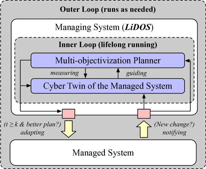
Figure 4: LiDOS architecture with a hierarchical feedback loop.

IV Experiment Setup

In this work, we seek to understand the following research questions (RQs):

• RQ1: Is being “dynamic” more beneficial than being “stationary” for SASs?

• RQ2: How effective is the adaptation achieved by LiDOS

• RQ3: How efficient for LiDOS to produce a promising adaptation plan?

We ask RQ1 to verify whether considering lifelong dynamic optimization for SASs is more necessary than its stationary counterpart where an optimization run is simply restarted in the planning. We study RQ2 to confirm the effectiveness of LiDOS against state-of-the-art planners. Yet, it would still be meaningless if LiDOS requires a large amount of planning overhead to become effective. Therefore, RQ3 seeks to understand how much speedup that LiDOS can achieve against the state-of-the-arts.

IV-A Subject SASs

We study three real-world SASs that are widely used in prior work of configurable and self-adaptive systems:

• Apache Storm: a distributed stream processing computation framework that executes a series of job batches. Adaptation means altering runtime options such as message_size, num_counters, and num_splitters. The changing environments are related to the workload and type of a given batch of jobs.

• Keras/DNN: the deep neural network (DNN) from the well-known Keras framework for classification tasks as part of a learning system. When deployed and trained, the learning system then classifies newly given samples. Adaptation refers to adjust options includes batch_size, num_filters, and log_decay, for (re-)training the network in the system. The environment can change depending on the given dataset for training.

• x264: A system for encoding videos. Adaptation means tuning runtime options includes no_mbtree, bframes, and ip_ratio. Environment is determined by the sizes and frames of different videos.

More detailed information about the SASs has been shown in Table I, where we consider two environments that can change at runtime for each SAS and use the same setting as previous work. Note that since the measurement of an adaptation plan can be expensive (even with a Cyber-Twin) [27], it is important to find an effective plan using as few measurements as possible. To expedite the experiment, we use the readily available dataset of those systems [3, 4, 34, 35] from existing work to emulate the Cyber-Twin of the managed system.

TABLE I: Real-world self-adaptive systems studied.

SAS	$\lvert\mathbfcal{P}\rvert$	Environment	$\lvert\mathbfcal{O}\rvert$	$\lvert\mathbfcal{S}\rvert$	Used By
Storm	Throughput	WordCount	12	1,914	[3, 4, 35]
		RollingCount
Keras/DNN	AUC	ShapesAll	12	16,384	[36, 34]
		Adiac
x264	Latency	128/44	17	53,662	[3, 37, 35]
		8/2

• $\lvert\mathbfcal{P}\rvert$, $\lvert\mathbfcal{O}\rvert$ and $\lvert\mathbfcal{S}\rvert$ denote performance objective, $\#$ adaptation options and search space, respectively.

IV-B Compared SAS Planners

To answer our RQs, we compare LiDOS with the following variants and state-of-the-art planners:

• LiDOS_sta : This is a stationary variant of the LiDOS, such that a simple restart is triggered whenever a change of environment is detected. All other parts are identical.

• Pseudo-dynamic planner (Ramirez et al. [12] & Kinneer et al. [15]): The planner uses a vanilla search algorithm that runs continuously over environmental changes, i.e., single-objective genetic algorithm (SOGA) [38], without tinkering how dynamics are handled during the search.

• Stationary planner (Chen et al. [9]): The planner where a new search run is triggered (with random initial adaptation plans) when an environment change is detected. This is similar to LiDOS_sta but without the multi-objectivization/NSGA-II and SOGA is used instead.

All planners are implemented in Java with search algorithms from jMetal [39]. Experiments are conducted on a machine with quad-core CPU at 2.8GHz and 16GB RAM.

IV-C Parameter Settings

For the key parameters of the stochastic search algorithm in all the planners, we apply the binary tournament for mating selection, together with the boundary mutation and uniformed crossover, as used in prior work for SASs [9, 40, 14]. The mutation and crossover rates are set to 0.1 and 0.9, respectively, with a population size of 20, which is widely used [9, 27].

To provide fair statistics for RQ1 and RQ2 (especially for those stationary counterparts), we set the adaptation interval $k$ as 150 measurements (of the Cyber-Twin), as it is the smallest number that there is no change on the best adaptation plan in the last 5 iterations (for all planners), implying a reasonable convergence. Clearer trajectories of the performance change over time will be demonstrated for RQ3.

IV-D Statistical Validation

To verify statistical significance, all experiments in this work are repeated 50 runs.

IV-D1 Pair-wise Comparisons

We use the following methods for comparing the target performance objective of two planners:

• Non-parametric test: To verify statistical significance, we leverage the Wilcoxon rank-sum test [41] — a widely used non-parametric test for SBSE and has been recommended in software engineering research for its strong statistical power on pairwise comparisons [42]. The standard $a=0.05$ is set as the significance level over 50 runs. If the $p<0.05$, we say the magnitude of differences in the comparisons are significant.

• Effect size: To ensure the resulted differences are not generated from a trivial effect, we use $\hat{A}_{12}$ [43] to verify the effect size over 50 runs. According to Vargha and Delaney [43], when comparing LiDOS and its counterpart in this work, $\hat{A}_{12}>0.5$ denotes that the LiDOS is better for more than 50% of the times. In particular, $0.56\leq\hat{A}_{12}<0.64$ indicates a small effect size while $0.64\leq\hat{A}_{12}<0.71$ and $\hat{A}_{12}\geq 0.71$ mean a medium and a large effect size, respectively.

As such, we say a comparison is statistically significant only if it has $\hat{A}_{12}\geq 0.56$ (or $\hat{A}_{12}\leq 0.44$) and $p<0.05$.

IV-D2 Three or More Comparisons

In case more than two planners need to be compared, we apply Scott-Knott test [44] on all comparisons on the target performance objective over 50 runs, as recommended by Mittas and Angelis [44]. In a nutshell, Scott-Knott sorts the list of treatments (the planners) by their median values of the target performance objective. Next, it splits the list into two sub-lists with the largest expected difference [45]. For example, suppose that we compare $A$, $B$, and $C$, a possible split could be: $\{A,B\}$, $\{C\}$, with the rank of 1 and 2, respectively. This means that, in the statistical sense, $A$ and $B$ perform similarly, but they are significantly better than $C$. Formally, Scott-Knott test aims to find the best split by maximizing the difference $\Delta$ in the expected mean before and after each split:

$$\Delta=\frac{|l_{1}|}{|l|}(\overline{l_{1}}-\overline{l})^{2}+\frac{|l_{2}|}{|l|}(\overline{l_{2}}-\overline{l})^{2}$$ (3)

whereby $|l_{1}|$ and $|l_{2}|$ are the sizes of two sub-lists ($l_{1}$ and $l_{2}$) from list $l$ with a size $|l|$. $\overline{l_{1}}$, $\overline{l_{2}}$, and $\overline{l}$ denote their mean values of the target performance objective.

During the splitting, we apply a statistical hypothesis test $H$ to check if $l_{1}$ and $l_{2}$ are significantly different. This is done by using bootstrapping and $\hat{A}_{12}$ [43]. If that is the case, Scott-Knott recurses on the splits. In other words, we divide the planners into different sub-lists if both bootstrap sampling and effect size test suggest that a split is statistically significant (with a confidence level of 99%) and with a good effect $\hat{A}_{12}\geq 0.6$. The sub-lists are then ranked based on their mean values of the target performance objective.

V Results

V-A RQ1: Benefit of Being “Dynamic”

V-A1 Method

To answer RQ1, we compare LiDOS and LiDOS_sta over changing environments under reasonable convergence of the planning. For each SAS, we run the system transits from one environment to another and set $k=150$. That is, for all planners, the planning is allowed to execute for 150 measurements and trigger an (better) adaptation. After the task in the current environment has been completed, the environment would be changed to another and the planner runs for a further 150 measurements before triggering the next adaptation. We report the target performance objective achieved by the last measurement. Wilcoxon rank-sum test and $\hat{A}_{12}$ are used for pair-wise comparisons over 50 runs.

V-A2 Result

As we can see from Table II, LiDOS wins all the 6 cases from which 4 of them have $p<0.05$ and at least medium effect size. The improvement in terms of median and IQR of the target performance objective has also been considerably high. Remarkably, it achieves almost $10\times$ median improvement on the case of x264 when the environment changes from the video with 128/44 to one with 8/2.

Since LiDOS and LiDOS_sta share the same optmization model and search algorithm, the above are clear evidence on the benefits of being dynamic when planning for SASs, as the stationary counterpart, which restarts the search upon environmental change, will waste the accumulated information that can be useful after the change. Therefore, we say:

TABLE II: Comparing LiDOS and the variant of LiDOS with a stationary setting (denotes as LiDOS_sta ) over 50 runs. max width=.1 visualizes the 25th, 50th, and 75th percentile of the results (normalized in the scale of all values found). $\hat{A}_{12}>0.5$ means LiDOS wins (highlighted in blue) while $\hat{A}_{12}<0.5$ denotes that it loses. Statistically significant comparisons are shown in bold. $\uparrow$ and $\downarrow$ denote maximal and minimal value of the performance objective is preferred, respectively; $\rightarrow$ indicates the direction of environment change at runtime.

max width = 1

Method	Median	IQR	$\hat{A}_{12}$ ($p$ value)
LiDOSsta	4803	206		max width=.1	$\uparrow$
LiDOS	4883	122	0.56 ($p=0.347$)	max width=.1
Throughput (msgs/min) for Storm, WordCount $\rightarrow$ RollingCount
Method	Median	IQR	$\hat{A}_{12}$ ($p$ value)
LiDOSsta	10119	56		max width=.1	$\uparrow$
LiDOS	10200	60	0.75 ($p<0.001$)	max width=.1
Throughput (msgs/min) for Storm, RollingCount $\rightarrow$ WordCount
Method	Median	IQR	$\hat{A}_{12}$ ($p$ value)
LiDOSsta	0.064	0.105		max width=.1	$\uparrow$
LiDOS	0.274	0.225	0.70 ($p=0.038$)	max width=.1
AUC for Keras/DNN, ShapesAll $\rightarrow$ Adaic
Method	Median	IQR	$\hat{A}_{12}$ ($p$ value)
LiDOSsta	0.178	0.278		max width=.1	$\uparrow$
LiDOS	0.292	0.292	0.58 ($p=0.167$)	max width=.1
AUC for Keras/DNN, Adaic $\rightarrow$ ShapesAll
Method	Median	IQR	$\hat{A}_{12}$ ($p$ value)
LiDOSsta	31.147	32.210		max width=.1	$\downarrow$
LiDOS	3.877	0.703	0.80 ($p<0.001$)	max width=.1
Latency (s) for x264, 128/44 $\rightarrow$ 8/2
Method	Median	IQR	$\hat{A}_{12}$ ($p$ value)
LiDOSsta	113.350	13.610		max width=.1	$\downarrow$
LiDOS	106.510	9.050	0.70 ($p<0.001$)	max width=.1
Latency (s) for x264, 8/2 $\rightarrow$ 128/44

V-B RQ2: Effectiveness of Adaptation

V-B1 Method

For RQ2, we compare LiDOS with the state-of-the-art pseudo-dynamic planner (Ramirez et al. [12] & Kinneer et al. [15]) and the stationary planner (Chen et al. [9]) discussed in Section IV-B. We use the same setting for environmental changes as that for RQ1 and report the results by the last measurement. Since there are more than two planners, we use Scott-Knott test to rank the results over 50 runs.

V-B2 Result

The results are reported in Table III. Clearly, LiDOS has been constantly ranked as the first with considerable improvement on the median performance over the others. Overall, the pseudo-dynamic planner by Ramirez et al. [12] & Kinneer et al. [15] tends to be better than the stationary one used by Chen et al. [9], but the improvement is not significant. This is not surprising, as the SOGA may be trapped at some undesired local optima, which tends to be not useful but misleading for the search after the environmental change.

To confirm the effectiveness of preserving different local optima for dynamic optimization in SAS planning, Figure 5 plots the performance of the adaptation plans found before and after the environmental change for one run of Storm. From Figure 5a, we see that the plans preserved by LiDOS right before the change occur contain a wide range of local optima (In fact, $c_{3}$ is the global optimum) — 6 out of 7 are the best among all their neighboring plans. In contrast, the pseudo-dynamic planner by Ramirez et al. [12] & Kinneer et al. [15] is more tempting to converge to one adaptation plan, which can be a local optimum. When re-measuring the same adaptation plans after the change (Figure 5b), we observe that:

TABLE III: Comparing LiDOS and the state-of-the-art pseudo-dynamic and stationary planners for SASs over 50 runs. In each case, the planners are sorted by Scott-Knott rank, median, and then IQR. The same formats as Table II applied.

max width = 1

Method	Rank	Median	IQR
LiDOS	1	4883	122	max width=.1	$\uparrow$
Ramirez et al. [12] & Kinneer et al. [15]	2	4761	0	max width=.1
Chen et al. [9]	2	4761	244	max width=.1
Throughput (msgs/min) for Storm, WordCount $\rightarrow$ RollingCount
Method	Rank	Median	IQR
LiDOS	1	10200	60	max width=.1	$\uparrow$
Ramirez et al. [12] & Kinneer et al. [15]	2	10140	21	max width=.1
Chen et al. [9]	2	10119	116	max width=.1
Throughput (msgs/min) for Storm, RollingCount $\rightarrow$ WordCount
Method	Rank	Median	IQR
LiDOS	1	0.274	0.225	max width=.1	$\uparrow$
Ramirez et al. [12] & Kinneer et al. [15]	1	0.174	0.233	max width=.1
Chen et al. [9]	2	0.059	0.113	max width=.1
AUC for Keras/DNN, ShapesAll $\rightarrow$ Adaic
Method	Rank	Median	IQR
LiDOS	1	0.292	0.292	max width=.1	$\uparrow$
Chen et al. [9]	2	0.163	0.258	max width=.1
Ramirez et al. [12] & Kinneer et al. [15]	2	0.112	0.245	max width=.1
AUC for Keras/DNN, Adaic $\rightarrow$ ShapesAll
Method	Rank	Median	IQR
LiDOS	1	3.877	0.703	max width=.1	$\downarrow$
Ramirez et al. [12] & Kinneer et al. [15]	1	4.190	26.247	max width=.1
Chen et al. [9]	2	6.663	32.307	max width=.1
Latency (s) for x264, 128/44 $\rightarrow$ 8/2
Method	Rank	Median	IQR
LiDOS	1	106.510	9.050	max width=.1	$\downarrow$
Ramirez et al. [12] & Kinneer et al. [15]	2	113.310	9.550	max width=.1
Chen et al. [9]	3	120.660	13.680	max width=.1
Latency (s) for x264, 8/2 $\rightarrow$ 128/44

1. LiDOS immediately obtain the best adaptation plans among those found by the state-of-the-arts, i.e., $c_{1}$ under LiDOS, which is merely one of the local optima that it found before the change in Figure 5a. This shows the usefulness of local optima for coping with the dynamic changes that occur in the planning of SASs.

2. Although the single plan found by Ramirez et al. [12] & Kinneer et al. [15] is promising before (the 2nd best in Figure 5a), it can be significantly worsen after the change (only the 7th best in Figure 5b). This reveals the importance of exploring and preserving a wide range of local optima.

3. The random plans in the stationary planner (Chen et al. [9]) are of generally worse performance than the other two.

As a result, we conclude that:

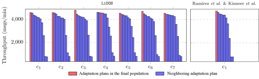
(a) Descendingly sorted performance of the preserved adaptation plans and their neighbouring plans before the change (RollingCount).

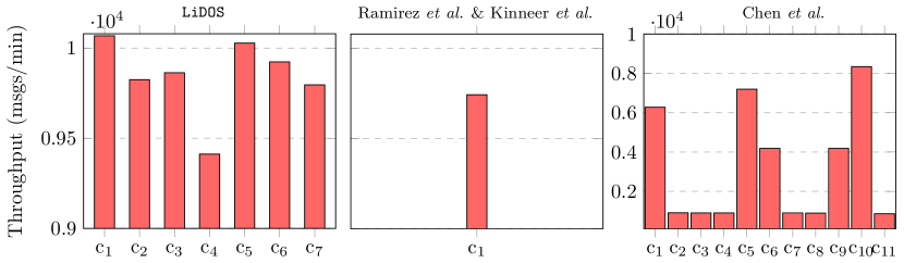
(b) Performance of the same preserved adaptation plans after the change (WordCount).

Figure 5: A run on the performance of preserved adaptation plans before and after the runtime environment change for Storm. (a) illustrates the performance of all plans found before the change and whether they are local optima with respect to their neighboring configurations; the x-axis indicates the unique plans. (b) shows the performance of the same unique plans after the change. The rightmost figure in (b) shows the result of the stationary planner by Chen et al. [9], which essentially are some randomly generated adaptation plans.

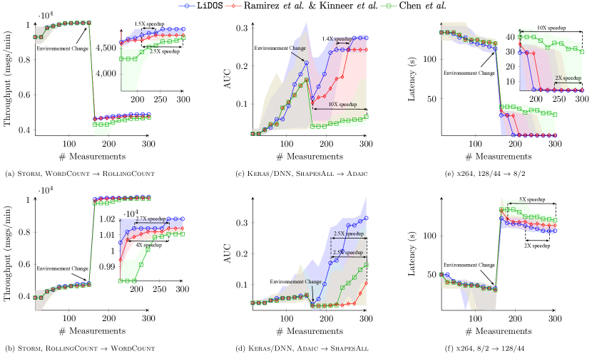
Figure 6: Trajectories of adaptation planning with environment change at runtime. The points and highlighted areas denote the median and IQR of the performance objective every 15 measurements over 50 runs, respectively. The small figures are “zoom-in” of the differences after the change in greater detail.

V-C RQ3: Efficiency of Adaptation

V-C1 Method

RQ1 and RQ2 have demonstrated the effectiveness and benefit of LiDOS under $k=150$ that leads to a reasonable convergence in the SAS planning. However, the results are less promising if LiDOS requires a generally higher planning overhead to achieve such. In RQ3, we investigate the trajectories of the target performance objective when planning across all measurements with the environmental change. We are particularly interested in the efficiency of adaptation after an environmental change: the “speedup” of LiDOS to reach the best performance as that achieved by the state-of-the-art. To this end, we use the metric of $T_{base}\over T_{LiDOS}$ proposed by Gao et al. [46], whereby $T_{base}$ is the smallest number of measurements (after change) for a state-of-the-art planner to obtain its best performance; $T_{LiDOS}$ is the smallest number of measurements (after change) for LiDOS to perform the same.

V-C2 Result

Figure 6 illustrates the results, from which we see that the environmental change indeed causes a severer disruption for the planning. However, thanks to the ability to preserve multiple local optima, LiDOS generally starts planning with some better adaptation plans than the state-of-the-art after an environmental change, hence leading to faster and better improvement throughout the planning. It is worth noting that such a benefit can be achieved even if the plans found before the change are not quite promising: while the LiDOS generally can better mitigate the issue of being trapped by local optima (thanks to MMO), there are still cases (e.g., Figure 6f) where its median is worse than the others. However, even in this case, the multi-objectivization planner in LiDOS can still lead to a better trajectory after an environmental change occurs.

When comparing the efficiency, we see that LiDOS achieves significant improvement over the others: $1.4\times$ to $5\times$ speedup over the pseudo-dynamic planner by Ramirez et al. [12] & Kinneer et al. [15]; $2.5\times$ to $10\times$ speedup on the stationary planner by Chen et al. [9].

In summary, we state that:

VI Threats to Validity

Threats to internal validity can be related to the $k$, which determines the time allowed for planning. We set $k=150$ in this work since we found that it reaches reasonable convergence for the SASs studied, i.e., for all planners, the best adaptation plan found does not change for the last 5 consecutive iterations. Further, in RQ3, we examine the trajectory of planning, which also indicates what would happen if a smaller $k$ is used. The other parameter settings follow what has been pragmatically used from the literature [9, 40, 14, 27]. However, we acknowledge that examining alternative parameters (and larger $k$) can be an interesting topic and we leave this for future work. To mitigate bias, we repeated 50 runs for each case.

The metrics and evaluation used may possess threats to construct validity. Since we focus on the scenario where there is only a single performance concern, we directly use the measured performance objective in the comparisons (for RQ1 and RQ2) and the formula of speedup used by Gao et al. [46] to evaluate the efficiency of planning (for RQ3). To verify statistical significance and effect size, we use Wilcoxon rank-sum test and $\hat{A}_{12}$ to examine the pairwise comparisons. When comparing more than two planners, we use Scott-Knott test for ranking. Yet, admittedly, measurement noises are possible.

The subject SASs and environments studied may contribute to the threats to external validity. We mitigated this by using 6 systems/environments that are of different domains, scales and performance attributes, as used by prior work [3, 4, 36, 34, 35]. We also compared LiDOS with its stationary variant and two state-of-the-art planners for SASs. Nonetheless, we agree that studying additional systems and other types of planners may prove fruitful.

VII Related Work

In this section, we discuss the related work in light of the concepts and design of LiDOS.

VII-A Stationary Optimization for SASs

In contrast to the dynamic (and pseudo-dynamic) optimization, stationary planners take a simpler strategy: the search is restarted from scratch whenever there is a new environmental change (or indeed a new search run under a fixed frequency) [9, 10, 11, 16, 47, 48, 49, 50]. Among other, Chen et al. [9] propose FEMOSAA, a framework that relies on stationary optimization for the SAS planning. While FEMOSAA is designed to make adaptation under a fixed frequency throughout the lifetime of SAS, the search and planning does not run continuously — every time the search restarts with some randomly generated adaptation plans. Elkhodary et al. [10] and Gerasimou et al. [11] also follow similar way with an exact/stochastic search, but the planning is conducted only when there is an environmental change or severe violation of performance requirement has been detected — yet again each time the search starts from scratch.

Clearly, stationary optimization ignores the information that could have been useful for the next planning, which makes the issues of local optima more difficult to address. With LiDOS, we seek to better exploit such information to improve the effectiveness and efficiency of SAS planning.

VII-B Dynamic Optimization for SASs

Dynamic optimization for SASs has been traditionally referred to the fact that a vanilla search algorithm runs continuously for planning [12, 13, 14, 15]. For example, Ramirez et al. [12] design Plato, a framework that adopts SOGA for SAS planning. They have shown that without specific designs, SOGA can deal with environmental change by detecting the changes in fitness. As such, Plato meets the concept of lifelong optimization. A similar notion that has been used for SASs is seeding — the planning and search are “seeded” by adaptation plans from previous runs of planning [13, 14]. Kinneer et al. [15] follows such a scheme using SOGA for searching in the SAS planner. Conceptually, seeding is similar to running the search and planning continuously and thus is referred to as dynamic optimization for SASs in the literature.

Although the search algorithm is dynamic in nature, the above differs from the true definition of dynamic optimization in the literature [26]. This is because no specific mechanism has been designed to handle the possible landscape change as the search proceeds, but leaving with the hopes that the algorithm would eventually cope with those changes in some ways. Therefore, the above work can be considered as pseudo-dynamic, and hence the information that can be leveraged after environment change is limited. In contrast, LiDOS contains the refined MMO, which is used and designed explicitly to address the formulated multi-modal optimization problem by taking the characteristics of SAS planning into account, aiming to better handle the dynamic changes as the planning runs. As we have shown, preserving multiple local optima (without harming the tendency towards the global optimum) can indeed provide more useful information than simply detecting the changing values of performance objective when the environment changes.

VII-C Control Theoretical Planning

Apart from the SBSE, control theoretical approaches have also been applied for SAS planning [17, 18, 19]. Among others, Maggio et al. [18] use Kalman filter to revise and update the state values of the controller model, where the core is a model predictive control scheme. Shevtsov and Weyns [19] also adopt a control theoretical approach, but they extend such with the simplex optimization method, which is essentially a kind of search algorithm.

We consider the contributions in this work as being complementary to the control theoretical planners rather than competitive, because fundamentally the purpose of search and optimization is to seek the global optimum. As a result, LiDOS can be integrated with a control theoretical planner such that it seeks to find the global optimum of the current system state modeled by the controller, similar to what has been done by Shevtsov and Weyns [19].

VII-D Performance Learning for SASs

Another relevant thread of research is performance learning for configurable systems. Various methods have been used, such as neural network [20, 21], linear regression [20], ensemble learning [23] and transfer learning [25]. However, the aim is to learn an accurate function that captures the correlation between adaptation options and the performance while we target planning, therefore our contributions are orthogonal to the above. For example, with an accurate performance model, the Cyber-Twin in LiDOS can be replaced by such a model, achieving faster measurements and hence boosting the planning.

VIII Conclusion

This paper presents LiDOS, a lifelong and truly dynamic optimization framework with a hierarchical feedback loop architecture for SAS planning. We formulate the lifelong dynamic optimization for SAS as a multi-modal optimization problem, which is solved by the refined meta multi-objectivization (MMO) model. The aim is to preserve as many local optima as possible without harming the tendency towards the global optimum, hence providing useful information for planning after the environmental change.

Experiments on three diverse real-world SASs and different environmental changes show that compared with the stationary counterpart and other state-of-the-art planners, LiDOS is:

• more effective, as it achieves considerably better adaptation plan than the stationary counterparts and other state-of-the-art planners with up to $10\times$ improvement;

• and more efficient, since it exhibits $1.4\times$ to $10\times$ speedup on producing promising plans.

This work is among the first attempt to explicitly handle the “dynamic” on landscape changes during the run of the search for SAS planning. We show that such a lifelong dynamic optimization is factual for planning in SAS, which can excite a few future research directions, such as considering information from all previous planning runs and memory mechanisms to more precisely track the details of landscape changes between different environments.

References

- [1] L. Lesoil, M. Acher, X. Tërnava, A. Blouin, and J. Jézéquel, “The interplay of compile-time and run-time options for performance prediction,” in SPLC ’21: 25th ACM International Systems and Software Product Line Conference, Leicester, United Kingdom, September 6-11, 2021, Volume A, M. Mousavi and P. Schobbens, Eds. ACM, 2021, pp. 100–111. [Online]. Available: https://doi.org/10.1145/3461001.3471149
- [2] T. Chen, R. Bahsoon, and X. Yao, “A survey and taxonomy of self-aware and self-adaptive cloud autoscaling systems,” ACM Comput. Surv., vol. 51, no. 3, pp. 61:1–61:40, 2018. [Online]. Available: https://doi.org/10.1145/3190507
- [3] V. Nair, Z. Yu, T. Menzies, N. Siegmund, and S. Apel, “Finding faster configurations using flash,” IEEE Transactions on Software Engineering, vol. 46, no. 7, 2020.
- [4] P. Jamshidi and G. Casale, “An uncertainty-aware approach to optimal configuration of stream processing systems,” in 24th IEEE International Symposium on Modeling, Analysis and Simulation of Computer and Telecommunication Systems, MASCOTS 2016, London, United Kingdom, September 19-21, 2016. IEEE Computer Society, 2016, pp. 39–48.
- [5] R. de Lemos, H. Giese, H. A. Müller, M. Shaw, J. Andersson, M. Litoiu, B. R. Schmerl, G. Tamura, N. M. Villegas, T. Vogel, D. Weyns, L. Baresi, B. Becker, N. Bencomo, Y. Brun, B. Cukic, R. J. Desmarais, S. Dustdar, G. Engels, K. Geihs, K. M. Göschka, A. Gorla, V. Grassi, P. Inverardi, G. Karsai, J. Kramer, A. Lopes, J. Magee, S. Malek, S. Mankovski, R. Mirandola, J. Mylopoulos, O. Nierstrasz, M. Pezzè, C. Prehofer, W. Schäfer, R. D. Schlichting, D. B. Smith, J. P. Sousa, L. Tahvildari, K. Wong, and J. Wuttke, “Software engineering for self-adaptive systems: A second research roadmap,” in Software Engineering for Self-Adaptive Systems II - International Seminar, Dagstuhl Castle, Germany, October 24-29, 2010 Revised Selected and Invited Papers, ser. Lecture Notes in Computer Science, R. de Lemos, H. Giese, H. A. Müller, and M. Shaw, Eds., vol. 7475. Springer, 2010, pp. 1–32. [Online]. Available: https://doi.org/10.1007/978-3-642-35813-5_1
- [6] T. Chen, R. Bahsoon, and X. Yao, “Synergizing domain expertise with self-awareness in software systems: A patternized architecture guideline,” Proc. IEEE, vol. 108, no. 7, pp. 1094–1126, 2020. [Online]. Available: https://doi.org/10.1109/JPROC.2020.2985293
- [7] T. Chen, R. Bahsoon, S. Wang, and X. Yao, “To adapt or not to adapt?: Technical debt and learning driven self-adaptation for managing runtime performance,” in Proceedings of the 2018 ACM/SPEC International Conference on Performance Engineering, ICPE 2018, Berlin, Germany, April 09-13, 2018, K. Wolter, W. J. Knottenbelt, A. van Hoorn, and M. Nambiar, Eds. ACM, 2018, pp. 48–55. [Online]. Available: https://doi.org/10.1145/3184407.3184413
- [8] T. Chen, M. Li, K. Li, and K. Deb, “Search-based software engineering for self-adaptive systems: Survey, disappointments, suggestions and opportunities,” arXiv preprint arXiv:2001.08236, 2020.
- [9] T. Chen, K. Li, R. Bahsoon, and X. Yao, “FEMOSAA: Feature guided and knee driven multi-objective optimization for self-adaptive software,” ACM Transactions on Software Engineering and Methodology, vol. 27, no. 2, 2018.
- [10] A. M. Elkhodary, N. Esfahani, and S. Malek, “FUSION: a framework for engineering self-tuning self-adaptive software systems,” in Proceedings of the 18th ACM SIGSOFT International Symposium on Foundations of Software Engineering, 2010, Santa Fe, NM, USA, November 7-11, 2010, G. Roman and A. van der Hoek, Eds. ACM, 2010, pp. 7–16. [Online]. Available: https://doi.org/10.1145/1882291.1882296
- [11] S. Gerasimou, R. Calinescu, and G. Tamburrelli, “Synthesis of probabilistic models for quality-of-service software engineering,” Autom. Softw. Eng., vol. 25, no. 4, pp. 785–831, 2018. [Online]. Available: https://doi.org/10.1007/s10515-018-0235-8
- [12] A. J. Ramirez, D. B. Knoester, B. H. C. Cheng, and P. K. McKinley, “Applying genetic algorithms to decision making in autonomic computing systems,” in Proceedings of the 6th International Conference on Autonomic Computing, ICAC 2009, June 15-19, 2009, Barcelona, Spain, S. A. Dobson, J. Strassner, M. Parashar, and O. Shehory, Eds. ACM, 2009, pp. 97–106. [Online]. Available: https://doi.org/10.1145/1555228.1555258
- [13] T. Chen, M. Li, and X. Yao, “On the effects of seeding strategies: a case for search-based multi-objective service composition,” in Proceedings of the Genetic and Evolutionary Computation Conference, GECCO 2018, Kyoto, Japan, July 15-19, 2018, H. E. Aguirre and K. Takadama, Eds. ACM, 2018, pp. 1419–1426. [Online]. Available: https://doi.org/10.1145/3205455.3205513
- [14] ——, “Standing on the shoulders of giants: Seeding search-based multi-objective optimization with prior knowledge for software service composition,” Inf. Softw. Technol., vol. 114, pp. 155–175, 2019. [Online]. Available: https://doi.org/10.1016/j.infsof.2019.05.013
- [15] C. Kinneer, D. Garlan, and C. L. Goues, “Information reuse and stochastic search: Managing uncertainty in self- systems,” ACM Trans. Auton. Adapt. Syst., vol. 15, no. 1, pp. 3:1–3:36, 2021. [Online]. Available: https://doi.org/10.1145/3440119
- [16] S. Kumar, T. Chen, R. Bahsoon, and R. Buyya, “DATESSO: self-adapting service composition with debt-aware two levels constraint reasoning,” in SEAMS ’20: IEEE/ACM 15th International Symposium on Software Engineering for Adaptive and Self-Managing Systems, Seoul, Republic of Korea, 29 June - 3 July, 2020, S. Honiden, E. D. Nitto, and R. Calinescu, Eds. ACM, 2020, pp. 96–107. [Online]. Available: https://doi.org/10.1145/3387939.3391604
- [17] A. Filieri, H. Hoffmann, and M. Maggio, “Automated multi-objective control for self-adaptive software design,” in Proceedings of the 2015 10th Joint Meeting on Foundations of Software Engineering, ESEC/FSE 2015, Bergamo, Italy, August 30 - September 4, 2015, E. D. Nitto, M. Harman, and P. Heymans, Eds. ACM, 2015, pp. 13–24. [Online]. Available: https://doi.org/10.1145/2786805.2786833
- [18] M. Maggio, A. V. Papadopoulos, A. Filieri, and H. Hoffmann, “Automated control of multiple software goals using multiple actuators,” in Proceedings of the 2017 11th Joint Meeting on Foundations of Software Engineering, ESEC/FSE 2017, Paderborn, Germany, September 4-8, 2017, E. Bodden, W. Schäfer, A. van Deursen, and A. Zisman, Eds. ACM, 2017, pp. 373–384. [Online]. Available: https://doi.org/10.1145/3106237.3106247
- [19] S. Shevtsov and D. Weyns, “Keep it SIMPLEX: satisfying multiple goals with guarantees in control-based self-adaptive systems,” in Proceedings of the 24th ACM SIGSOFT International Symposium on Foundations of Software Engineering, FSE 2016, Seattle, WA, USA, November 13-18, 2016, T. Zimmermann, J. Cleland-Huang, and Z. Su, Eds. ACM, 2016, pp. 229–241. [Online]. Available: https://doi.org/10.1145/2950290.2950301
- [20] T. Chen and R. Bahsoon, “Self-adaptive and sensitivity-aware qos modeling for the cloud,” in Proceedings of the 8th International Symposium on Software Engineering for Adaptive and Self-Managing Systems, SEAMS 2013, San Francisco, CA, USA, May 20-21, 2013, M. Litoiu and J. Mylopoulos, Eds. IEEE Computer Society, 2013, pp. 43–52. [Online]. Available: https://doi.org/10.1109/SEAMS.2013.6595491
- [21] H. Ha and H. Zhang, “Deepperf: performance prediction for configurable software with deep sparse neural network,” in Proceedings of the 41st International Conference on Software Engineering, ICSE 2019, Montreal, QC, Canada, May 25-31, 2019, J. M. Atlee, T. Bultan, and J. Whittle, Eds. IEEE / ACM, 2019, pp. 1095–1106. [Online]. Available: https://doi.org/10.1109/ICSE.2019.00113
- [22] T. Chen, R. Bahsoon, and X. Yao, “Online qos modeling in the cloud: A hybrid and adaptive multi-learners approach,” in Proceedings of the 7th IEEE/ACM International Conference on Utility and Cloud Computing, UCC 2014, London, United Kingdom, December 8-11, 2014. IEEE Computer Society, 2014, pp. 327–336. [Online]. Available: https://doi.org/10.1109/UCC.2014.42
- [23] T. Chen and R. Bahsoon, “Self-adaptive and online qos modeling for cloud-based software services,” IEEE Trans. Software Eng., vol. 43, no. 5, pp. 453–475, 2017. [Online]. Available: https://doi.org/10.1109/TSE.2016.2608826
- [24] T. Chen, “All versus one: an empirical comparison on retrained and incremental machine learning for modeling performance of adaptable software,” in Proceedings of the 14th International Symposium on Software Engineering for Adaptive and Self-Managing Systems, SEAMS@ICSE 2019, Montreal, QC, Canada, May 25-31, 2019, M. Litoiu, S. Clarke, and K. Tei, Eds. ACM, 2019, pp. 157–168. [Online]. Available: https://doi.org/10.1109/SEAMS.2019.00029
- [25] P. Jamshidi, N. Siegmund, M. Velez, C. Kästner, A. Patel, and Y. Agarwal, “Transfer learning for performance modeling of configurable systems: an exploratory analysis,” in Proceedings of the 32nd IEEE/ACM International Conference on Automated Software Engineering, ASE 2017, Urbana, IL, USA, October 30 - November 03, 2017, G. Rosu, M. D. Penta, and T. N. Nguyen, Eds. IEEE Computer Society, 2017, pp. 497–508. [Online]. Available: https://doi.org/10.1109/ASE.2017.8115661
- [26] T. T. Nguyen, S. Yang, and J. Branke, “Evolutionary dynamic optimization: A survey of the state of the art,” Swarm Evol. Comput., vol. 6, pp. 1–24, 2012. [Online]. Available: https://doi.org/10.1016/j.swevo.2012.05.001
- [27] T. Chen and M. Li, “Multi-objectivizing software configuration tuning,” in ESEC/FSE ’21: 29th ACM Joint European Software Engineering Conference and Symposium on the Foundations of Software Engineering, Athens, Greece, August 23-28, 2021, D. Spinellis, G. Gousios, M. Chechik, and M. D. Penta, Eds. ACM, 2021, pp. 453–465. [Online]. Available: https://doi.org/10.1145/3468264.3468555
- [28] M. Harman, S. A. Mansouri, and Y. Zhang, “Search-based software engineering: Trends, techniques and applications,” ACM Computing Surveys (CSUR), vol. 45, no. 1, p. 11, 2012.
- [29] O. Mersmann, B. Bischl, H. Trautmann, M. Preuss, C. Weihs, and G. Rudolph, “Exploratory landscape analysis,” in 13th Annual Genetic and Evolutionary Computation Conference, GECCO 2011, Proceedings, Dublin, Ireland, July 12-16, 2011, N. Krasnogor and P. L. Lanzi, Eds. ACM, 2011, pp. 829–836. [Online]. Available: https://doi.org/10.1145/2001576.2001690
- [30] J. Tavares, F. B. Pereira, and E. Costa, “Multidimensional knapsack problem: A fitness landscape analysis,” IEEE Trans. Syst. Man Cybern. Part B, vol. 38, no. 3, pp. 604–616, 2008. [Online]. Available: https://doi.org/10.1109/TSMCB.2008.915539
- [31] G. Singh and K. Deb, “Comparison of multi-modal optimization algorithms based on evolutionary algorithms,” in Genetic and Evolutionary Computation Conference, GECCO 2006, Proceedings, Seattle, Washington, USA, July 8-12, 2006, M. Cattolico, Ed. ACM, 2006, pp. 1305–1312. [Online]. Available: https://doi.org/10.1145/1143997.1144200
- [32] K. Deb, A. Pratap, S. Agarwal, and T. Meyarivan, “A fast and elitist multiobjective genetic algorithm: Nsga-ii,” IEEE Transactions on Evolutionary Computation, vol. 6, no. 2, pp. 182–197, 2002.
- [33] M. Salehie and L. Tahvildari, “Self-adaptive software: Landscape and research challenges,” ACM Trans. Auton. Adapt. Syst., vol. 4, no. 2, pp. 14:1–14:42, 2009. [Online]. Available: https://doi.org/10.1145/1516533.1516538
- [34] P. Jamshidi, M. Velez, C. Kästner, and N. Siegmund, “Learning to sample: exploiting similarities across environments to learn performance models for configurable systems,” in Proceedings of the 2018 ACM Joint Meeting on European Software Engineering Conference and Symposium on the Foundations of Software Engineering, ESEC/SIGSOFT FSE 2018, Lake Buena Vista, FL, USA, November 04-09, 2018, G. T. Leavens, A. Garcia, and C. S. Pasareanu, Eds. ACM, 2018, pp. 71–82. [Online]. Available: https://doi.org/10.1145/3236024.3236074
- [35] K. Peng, C. Kaltenecker, N. Siegmund, S. Apel, and T. Menzies, “VEER: disagreement-free multi-objective configuration,” CoRR, vol. abs/2106.02716, 2021. [Online]. Available: https://arxiv.org/abs/2106.02716
- [36] P. Mendes, M. Casimiro, P. Romano, and D. Garlan, “Trimtuner: Efficient optimization of machine learning jobs in the cloud via sub-sampling,” in 28th International Symposium on Modeling, Analysis, and Simulation of Computer and Telecommunication Systems, MASCOTS 2020, Nice, France, November 17-19, 2020. IEEE, 2020, pp. 1–8. [Online]. Available: https://doi.org/10.1109/MASCOTS50786.2020.9285971
- [37] N. Siegmund, S. S. Kolesnikov, C. Kästner, S. Apel, D. S. Batory, M. Rosenmüller, and G. Saake, “Predicting performance via automated feature-interaction detection,” in 34th International Conference on Software Engineering, ICSE 2012, June 2-9, 2012, Zurich, Switzerland, M. Glinz, G. C. Murphy, and M. Pezzè, Eds. IEEE Computer Society, 2012, pp. 167–177. [Online]. Available: https://doi.org/10.1109/ICSE.2012.6227196
- [38] D. Whitley, “A genetic algorithm tutorial,” Statistics and computing, vol. 4, no. 2, pp. 65–85, 1994.
- [39] J. J. Durillo and A. J. Nebro, “jmetal: A java framework for multi-objective optimization,” Adv. Eng. Softw., vol. 42, no. 10, pp. 760–771, 2011. [Online]. Available: https://doi.org/10.1016/j.advengsoft.2011.05.014
- [40] A. Shahbazian, S. Karthik, Y. Brun, and N. Medvidovic, “equal: informing early design decisions,” in ESEC/FSE ’20: 28th ACM Joint European Software Engineering Conference and Symposium on the Foundations of Software Engineering, Virtual Event, USA, November 8-13, 2020, P. Devanbu, M. B. Cohen, and T. Zimmermann, Eds. ACM, 2020, pp. 1039–1051. [Online]. Available: https://doi.org/10.1145/3368089.3409749
- [41] F. Wilcoxon, “Individual comparisons by ranking methods,” 1945.
- [42] A. Arcuri and L. C. Briand, “A practical guide for using statistical tests to assess randomized algorithms in software engineering,” in ICSE’11: Proc. of the 33rd International Conference on Software Engineering. ACM, 2011, pp. 1–10.
- [43] A. Vargha and H. D. Delaney, “A critique and improvement of the cl common language effect size statistics of mcgraw and wong,” 2000.
- [44] N. Mittas and L. Angelis, “Ranking and clustering software cost estimation models through a multiple comparisons algorithm,” IEEE Trans. Software Eng., vol. 39, no. 4, pp. 537–551, 2013. [Online]. Available: https://doi.org/10.1109/TSE.2012.45
- [45] T. Xia, R. Krishna, J. Chen, G. Mathew, X. Shen, and T. Menzies, “Hyperparameter optimization for effort estimation,” CoRR, vol. abs/1805.00336, 2018. [Online]. Available: http://arxiv.org/abs/1805.00336
- [46] Y. Gao, Y. Zhu, H. Zhang, H. Lin, and M. Yang, “Resource-guided configuration space reduction for deep learning models,” in 43rd IEEE/ACM International Conference on Software Engineering, ICSE 2021, Madrid, Spain, 22-30 May 2021. IEEE, 2021, pp. 175–187. [Online]. Available: https://doi.org/10.1109/ICSE43902.2021.00028
- [47] S. Kumar, R. Bahsoon, T. Chen, K. Li, and R. Buyya, “Multi-tenant cloud service composition using evolutionary optimization,” in 24th IEEE International Conference on Parallel and Distributed Systems, ICPADS 2018, Singapore, December 11-13, 2018. IEEE, 2018, pp. 972–979. [Online]. Available: https://doi.org/10.1109/PADSW.2018.8644640
- [48] K. Li, Z. Xiang, T. Chen, and K. C. Tan, “Bilo-cpdp: Bi-level programming for automated model discovery in cross-project defect prediction,” in 35th IEEE/ACM International Conference on Automated Software Engineering, ASE 2020, Melbourne, Australia, September 21-25, 2020. IEEE, 2020, pp. 573–584. [Online]. Available: https://doi.org/10.1145/3324884.3416617
- [49] T. Chen and R. Bahsoon, “Self-adaptive trade-off decision making for autoscaling cloud-based services,” IEEE Trans. Serv. Comput., vol. 10, no. 4, pp. 618–632, 2017. [Online]. Available: https://doi.org/10.1109/TSC.2015.2499770
- [50] ——, “Symbiotic and sensitivity-aware architecture for globally-optimal benefit in self-adaptive cloud,” in 9th International Symposium on Software Engineering for Adaptive and Self-Managing Systems, SEAMS 2014, Proceedings, Hyderabad, India, June 2-3, 2014, G. Engels and N. Bencomo, Eds. ACM, 2014, pp. 85–94. [Online]. Available: https://doi.org/10.1145/2593929.2593931