Fragility Measures For Typical Cases

Abstract

The fragility index is a clinically motivated metric designed to supplement the $p$ value during hypothesis testing. The measure relies on two pillars: selecting cases to have their outcome modified and modifying the outcomes. The measure is interesting but the case selection suffers from a drawback which can hamper its interpretation. This work presents the drawback and a method, the stochastic generalized fragility indices, designed to remedy it. Two examples concerning electoral outcomes and the causal effect of smoking cessation illustrate the method.

Keywords: fragility index, hypothesis testing, interpretability, case selection, post-experimental evidence assessment, $p$ value, Bush v. Gore, reproducibility, ASA statements

1 Introduction

Null hypothesis significance testing has been the default route to establish the validity of scientific claims for generations. Throughout this time, the $p$ value has largely been the tool of choice for measuring the evidence against a null hypothesis. When properly applied and interpreted, the $p$ value increases the rigor of the conclusions drawn from data (Benjamini et al.,, 2021). Despite their ubiquity, the standard practice involving $p$ values suffers from several shortcomings. Two salient shortcomings are that $p$ values as a post-experimental evidence assessment are widely misunderstood (Wasserstein and Lazar,, 2016; Benjamini et al.,, 2021) and that the default threshold for significance ($p<0.05$) may not be stringent enough (Berger and Sellke,, 1987; Benjamin and Berger,, 2019).

1.1 The traditional fragility index

Towards resolving the two shortcomings of $p$ values, Walsh et al., (2014) proposed the fragility index, a measure which extends a variant proposed by Feinstein, (1990). Walsh et al., and Feinstein, were focused on analysing $2\times 2$ contingency tables which resulted from clinical trials. The (traditional) fragility index is formally defined in Definition 1 (Baer et al., 2021b, ).

Definition 1.

Consider data represented by a $2\times 2$ contingency table where the rows indicate intervention (treatment or control) arms and the columns indicate outcome (event or nonevent) status. The fragility index is the minimum number of cases whose outcomes must be modified to reverse statistical significance.

Note that this definition separates the algorithm and the implicit statistical method in Walsh et al., (2014), as argued by Lin, (2020) and Baer et al., 2021b .

The definition relies on a concept of statistical significance. In nearly all applications, this has been taken to correspond to the $p$ value from Fisher’s exact test being less than the default cutoff $0.05$. The definition then considers alternative contingency tables wherein each case can have a modified outcome. Although Walsh et al., (2014) defined the fragility index only for initially significant statistical tests, the measure was quickly and modestly extended to initially nonsignificant tests as well, via the so-called reverse fragility index (Johnson et al.,, 2017; Khan et al.,, 2020). While the fragility index was initially motivated by clinical applications Baer et al., 2021b ; Baer et al., 2021c suggest that it should be viewed as a trustworthy post-experimental evidence assessment that can be applied across the sciences. Towards this, we use the terminology case in place of patient throughout the article.

In many applications decisions are made on the basis of statistical significance determined by a critical threshold (Benjamini et al.,, 2021; Mayo,, 2021). Although, statistical significance is neither necessary nor sufficient for reaching a finding of material significance (Poole,, 1987; Goodman,, 1999, 2008; USSC,, 2010; Greenland et al.,, 2016). The intention of the fragility index is to provide a measure of the fragility of a statistical determination. The fragility index is an interpretable supplement to traditional measures of evidence like the $p$ value which is in terms of “case units” instead of probability units. The fragility index has been used to reanalyse the principal results in fields across medicine (Holek et al.,, 2020). Researchers in some fields have been realized that the statistical significance of practice-changing studies have hinged on the outcome of a particular patient (or case). This is especially troubling when that patient plausibly could have had a different outcome.

When researchers consider the value of the fragility index to determine whether a study’s conclusion is fragile, their action can be viewed as performing an informal statistical hypothesis test (Baer et al., 2021c, ). To make this clear, we must first update Definition 1: consider the fragility index to be the signed count of outcome modifications. Positive fragility indices correspond to initially significant tests, and negative fragility indices correspond to initially insignificant statistical tests. In a sense, this turns reverse fragility indices into negative fragility indices. This update is summarized in Definition 2.

Definition 2.

Throughout this article, we consider the fragility index to be a signed variant of Definition 1, so positive fragility indices correspond to initially significant tests, and a negative fragility indices correspond to initially insignificant tests.

With this improved measure, the fragility index can be neatly treated as a test statistic (Lehmann and Romano,, 2006). Suppose that we determine statistical significance through $p$ values. The fragility index being positive is equivalent to the $p$ value being less than the significance threshold. Therefore the fragility index provides an alternative test statistic for the same rejection region offered by a $p$ value (Baer et al., 2021c, ). This relationship is visualized in Figure 1. However, researchers commonly use the fragility index to go a step further. Indeed, the standard use case of the fragility index is to determine whether the fragility index of a statistically significant test is not “too low”, for otherwise the trial’s statistical conclusion would hinge on a small number of cases. This procedure amounts to comparing the fragility index to a positive threshold rather than merely $0$ and hence produces a more stringent statistical test with a lower type I error rate. The need for having a more stringent statistical test is further motivated by a lack of reproducibility: reversals of statistical conclusions can be surprisingly common in the medical literature (Herrera-Perez et al.,, 2019).

Figure 1: An intuitive depiction of the relationship between fragility indices (on top) and $p$ values (on bottom) when the $p$ value significance threshold is $0.05$. The scale depends on e.g. the sample size and effect size.

The concept underlying the fragility index is largely the same as the $p$ value. Both consider hypothetical outcomes from the same clinical trial. In one case, $p$ values rely on alternative case outcomes and their distributional impact on test statistics; in the other, the fragility indices directly explore alternative case outcomes.

Critiques of the fragility index have been reviewed by Baer et al., 2021b . As pointed out in the editorial that accompanied the ASA President’s Task Force Statement on the Statistical Significance and Replicability (Kafadar,, 2021), “[a] misuse of a tool ought not to lead to complete elimination of the tool from the toolbox, but rather to the development of better ways of communicating when it should, and should not, be used.”

We recommend Section 2 in Baer et al., 2021b for an elaborated development of the fragility index. Beyond the formalism of treating the fragility index as a test statistic, the fragility index can be neatly used in a sensitivity analysis.

1.2 The sample breakdown point

The theoretical basis of statistical science offers several general strategies for dealing with uncertainty in assessing significance (Benjamini et al.,, 2021), in this article we will connect some to important concepts from robust statistics. Baer et al., 2021b review an interesting connection between breakdown points from robust statistics and the fragility index quotient, i.e. the fragility index divided by the sample size (Ahmed et al.,, 2016).

We start by briefly reviewing the breakdown point in non-asymptotic settings. The breakdown point of an estimator is informally defined to be the smallest portion of distributional contamination such that a statistic diverges, i.e. breaks down (Hampel,, 1968; Hampel et al.,, 1986; Davies and Gather,, 2005). The distributional contamination can arise in several forms, and here we consider contamination in the form of observation replacement. A principal purpose of the breakdown point is to study the sensitivity of estimators to outliers. Breakdown points have analogously been defined for tests, and we formalize the definition in that context.

Several variants of test breakdown points have been developed (Rieder,, 1982; Simpson,, 1989; Jolliffe and Lukudu,, 1993); here we exclusively focus on measures where breaking down means statistical significance reverses. Measures connected to testing breakdown points are compared in Table 1, and in the remainder of this section we will explain the contents of the table. Ylvisaker, (1977) first studied the notion of breakdown for testing and defines the resistance of a test as the smallest fraction of observations that can always determine the test decision regardless of the other observations in the sample. Define $Z$ to be a data sample from $n$ cases and $I$ to be a subset of cases $\{1,\dots,n\}$. The maximum resistance (MR) is formally defined as the minimum cardinality $|I|/n$ such that for all ($\forall$) samples $Z,$   there exists ($\exists$) cases $I$ for which $\exists$ a modified sample $Z^{\textrm{mod}}$ which reverses significance, where $Z^{\textrm{mod}}$ only differs from the original sample $Z$ for cases in $I$ (Coakley and Hettmansperger,, 1994). This is indicated in the first column of Table 1. The maximum resistance tells how robust a test decision is for the least favorable sample and can be viewed as a least upper bound across all samples. Coakley and Hettmansperger, (1992) proposes the expected resistance (ER) of a test as a measure of the robustness of its decision through an average across samples with some specified distribution.

	MR	ER	S-BDP/FI	GFI-SL	SFI	SGFI-SL
Sample $Z$	$\forall$	Average	Given	Given	Given	Given
Selected cases $I$	$\exists$	$\exists$	$\exists$	$\exists$	$\exists$ typical	$\exists$ typical
Modified sample $Z^{\textrm{mod}}$	$\exists$	$\exists$	$\exists$	$\exists$ plausible	$\exists$	$\exists$ plausible

Table 1: A comparison of methods. The columns represent maximum resistance (MR), expected resistance (ER), sample breakdown point (S-BDP), fragility index (FI), generalized fragility index with the sufficiently likely construction (GFI-SL), stochastic fragility index (SFI), and stochastic generalized fragility index with the sufficiently likely construction (SGFI-SL), with cell entries there exists ($\exists$) and for all ($\forall$).

The maximum and expected resistances are defined across samples rather than for a given sample and are designed to study the abstract properties of statistical tests. On the other hand, in this article we are interested in studying a given a sample $Z$ (Donoho and Huber,, 1983). Zhang, (1996) introduced the first sample breakdown point (S-BDP) for testing, defined as the minimum $|I|/n$ such that $\,\exists$ cases $I$ for which $\exists$ a modified sample $Z^{\textrm{mod}}$ which reverses significance, where $Z^{\textrm{mod}}$ only differs from the original sample $Z$ for cases in $I$, for a given sample $Z$. Notice that when the sample $Z$ can be represented as a $2\times 2$ table, this is precisely the fragility index (Walsh et al.,, 2014) in Definition 1 divided by the sample size.

In our view the fragility index is intended to have a different purpose than breakdown points. Users of the fragility index tend to be interested in the impact of minor perturbations of the data on rejection decisions, for which the sample breakdown point is not suitable. When researchers report a small fragility index, they want the corresponding modifications to plausibly have occurred and not rely on extreme outliers. Baer et al., 2021b update the fragility index to explicitly be based on only likely modifications (which correspond to minor perturbations) through the generalized fragility indices (GFIs) with the sufficiently likely construction, as we review in Section 2.3.

Each of the measures discussed so far have a commonality. They merely ensure that existence of selected cases $I$ which contribute to reversing significance, as seen in the second row of Table 1. Donoho and Huber, (1983) suggest that this can be a shortcoming and discuss a measure that they call a stochastic sample breakdown point which randomly modifies outcomes. The methods we propose, the stochastic fragility index (SFI) and the stochastic generalized fragility indices (SGFIs), which rely on typical cases will be similar in spirit.

1.3 Motivation and roadmap

As seen in Table 1, the fragility index relies on two components which characterize the measure. The first is modifying outcomes. Baer et al., 2021b thoroughly studied this through the sufficiently likely construction. The second is selecting cases whose outcomes are to be modified. According to Definitions 1 and 2, the selected cases for the fragility index are the most extreme possible. We will see that these cases are atypical, which can hamper their interpretation.

In Section 2 we introduce methods to generalize and improve the selection of cases. In Section 3 we give real data examples which help develop intuition for the methods. Finally we summarise and conclude in Section 4.

2 Methods

We start with a motivating example. Consider the data on the left in Table 2 as arising from a simulated clinical trial. The original data has $p$ value $<0.01$ and the modified data has $p$ value $0.06$. The data is initially statistically significant and then becomes nonsignificant, with significance threshold $0.05$. The tables help show that the fragility index is $-7$: there exists seven cases for which statistical significance would be reversed had their outcomes been different.

	Event	Nonevent
Treatment	20	380
Control	15	385

	Event	Nonevent
Treatment	20	380
Control	8	392

Table 2: (Left) Simulated summary statistics; (Right) The modified data which reverses statistical significance

Because such little information is presented for each case–only their treatment arm and a dichotomous outcome–we can readily interpret these seven cases. Each received the control and had an event. Therefore we can refine our earlier fragility index interpretation: Seven cases who were in the control arm and experienced an event having a different outcome would have reversed significance.

However, interest may not lie in these particular cases. There are only $15$ such cases out of $800$ study participants, resulting in the modified cases being atypical enough that they represent only $\frac{15}{800}\times 100\%\approx 1.9\%$ of the study. A user of the fragility index may reasonably be interested in exploring the impact of typical study participants having alternative outcomes. Additionally, the cases may not be so readily interpretable in studies with more complicated data types.

In this section we introduce a method which relies on typical cases that we call the stochastic fragility indices. The method will resolve the interpretation issue motivated above, and we will plainly see through an example in Section 3.1 that the stochastic fragility indices take into account the rarity of the modified cases. This is further illustrated in Section 2.2. Note that the motivation underlying the stochastic fragility indices was described as an interesting direction to pursue in Baer et al., 2021b . After, we review the generalized fragility indices introduced in Baer et al., 2021b and extend the stochastic fragility indices. A second example in Section 3.2 illustrates that the study participants whose outcomes are modified in the generalized fragility index can be acutely atypical when additional covariates are analysed. Finally, we introduce an accompanying algorithm in Section 2.4 that is implemented in the open source R package FragilityTools (Baer et al., 2021a, ).

2.1 The stochastic fragility indices

In this section we define a method for $2\times 2$ contingency tables which relies on typical cases. We first present a revealing characterization of the fragility index and then leverage it to define the stochastic fragility indices.

By construction, the fragility index only guarantees the existence of cases for which significance would be reversed had their outcomes been different. We can see this by Definition 1 since the minimum could be achieved by only one collection of cases. Note that for $2\times 2$ tables, often more than only one collection of cases exist. The motivating example based on Table 2 illustrates this: any 7 cases could be chosen to reverse significance among the 15 control arm cases who experienced an event.

When the fragility index equals $k$, there exists a collection of $k$ cases for which significance would reverse had their outcomes been different. There are however several possible collections of cases; when there are $n$ cases, there are $\binom{n}{k}$ collections. For example, when $n=800$ and $k=7$, there are more than $4\times 10^{16}$ case collections. Of all these collections, the one collection of cases guaranteed to have outcomes which can reverse significance can be unusual.

We now introduce a fragility measure which does not necessarily rely on atypical cases.

Definition 3.

Define the stochastic fragility index $\mathrm{SFI}_{r}$ with threshold $r\in[0,1)$ as the minimum $k$ such that more than $r\times 100\%$ of case collections with cardinality $k$ have the reversibility property, that statistical significance can reverse had the cases in the collection had different outcomes.

Consider the stochastic fragility index to be signed according to the initial significance of the statistical test, as in Definition 2. The stochastic fragility indices can ensure that a substantial portion of possible case collections can reverse significance and hence is not forced to rely on atypical cases.

When $r=0$, the stochastic fragility index reduces to the fragility index in Definition 1. The same holds when $r<1/\binom{n}{\mathit{FI}}$, where $\mathit{FI}$ is the traditional fragility index. The stochastic fragility index is undefined when $r=1$. For convenience, we will abuse notation and write $\mathit{SFI}_{1}=\mathit{SFI}_{r}$, when $r=1^{-}$ is the limit as $r$ approaches $1$ from below. In this case, the stochastic fragility index ensures that all case collections with cardinality $\mathrm{SFI}_{r}$ have the reversibility property. We consider this to be a conservative value. Roughly speaking, in addition to relying on atypical cases, the measure will also rely on atypical cases at the opposite extreme.

When $r=1/2$, more than half of the possible case collections have the reversibility property. That is, most combinations of patients have possible outcomes which can reverse significance. We consider this to be a highly interpretable choice and treat it as the default.

The stochastic fragility index generalizes the fragility index to ensure that a particular pattern or collection of cases alone do not determine the fragility index result, analogously to the relationship between the stochastic sample breakdown point and the sample breakdown point. The stochastic fragility index can equivalently be defined as a quantile with respect to the discrete uniform distribution on the set of case collections with a given cardinality, as is explored in Section 2.4. With this view, the relationship between maximum resistance and expected resistance roughly corresponds to the relationship between fragility indices and stochastic fragility indices.

2.2 Interpreting the stochastic fragility indices

Interpretability is the beating heart of fragility measures. In this section, we study the interpretation of stochastic fragility indices for various choices of $r$. We focus on the case that $\mathit{SFI}_{r}=1$ since it is particularly intuitive: case collections reduce to merely cases.

We consider each of the following possible interpretations. The statistical test would not have been significant if:

1. a particular case had a different outcome,

2. a typical case had a different outcome, or

3. any single case had a different outcome.

When $r=0$ so that the stochastic fragility index is simply the traditional fragility index, the correct interpretation is the first. By construction, the fragility index only ensures the existence of cases which can reverse significance. When $r=1$, the correct interpretation of the stochastic fragility index is the third. Significance would reverse if any case had a different outcome, and the word “single” considers the multiplicity of cases and not which case. When $r=1/2$, we consider the correct interpretation of the stochastic fragility index to be the second. By definition, more than half of the cases in the study have the property that statistical significance would reverse had their outcome (alone) been different. In our view, more than half of the cases in a study cannot be atypical, so one of those cases must be typical.

Interpretations for $\mathit{SFI}_{r}>1$ are analogous except with case collections instead of individual cases. An example in Section 3.1 illustrates an interesting connection between case collections and the proportion of individual cases with a desirable property.

2.3 The stochastic generalized fragility indices

The generalized fragility indices directly extend the scope of the fragility index in Definition 1 to arbitrary data types and tests (Baer et al., 2021b, ). Let $Z$ be a data frame where the rows represent cases $(1,\dots,n)$ and the columns represent measurements. For the $2\times 2$ contingency tables described earlier, this data frame $Z$ stores the same data but in a long format. Let the function $m$ be the so-called outcome modifier which inputs a row of $Z$ and outputs the set of permitted modifications.

Writing $\mathcal{R}$ as the rejection region, the generalized fragility indices are formally defined as

$$\min\,\,\,\, \|Z-Z^{\mathrm{mod}}\|_{\#}$$ (1)

such that $$Z\in\mathcal{R}\,\oplus\,Z^{\textrm{mod}}\in\mathcal{R}$$

$$Z^{\textrm{mod}}_{i,}\in m(Z_{i,})\text{ for all }i=1,\dots,n$$

where $\oplus$ is the exlusive-or denoting that $Z$ or $Z^{\textrm{mod}}$ is in the rejection region (but not both) and $\|\cdot\|_{\#}$ is the norm which counts the number of nonzero rows, i.e. the number of cases with modified values for their measurements. This definition can be interpreted as a projection of the data, making clear the extreme nature of the generalized fragility index. As in Definition 2, consider the generalized fragility indices to be signed according to the initial significance. We can readily see that the generalized fragility indices do indeed generalize the fragility index for $2\times 2$ tables.

The outcome modifier $m$ needs to be chosen to define a generalized fragility index. We will choose $m$ according to the sufficiently likely construction (Baer et al., 2021b, ), which only permits outcome modifications that have probability at least $q$ for some user supplied $q\in[0,1]$. Thus the modifier $m=m_{q}$. We use the notation $\mathit{GFI}_{q}$ for these fragility measures. The sufficiently likely construction alleviates an issue with the traditional fragility index which strains its interpretation.

In this section, we marry the stochastic fragility indices and the generalized fragility indices to define a fragility measure which both relies on typical cases and permits only plausible modifications. The method will depend on two parameters: the threshold $r$ which controls how typical the cases who reverse significance must be and the sufficiently likely threshold $q$ which controls the plausibility of the modifications.

Definition 4.

Define the stochastic generalized fragility indices $\mathrm{SGFI}_{r,q}$ with thresholds $r\in[0,1)$ and $q\in[0,1]$ as the minimum $k$ such that more than $r\times 100\%$ of case collections with cardinality $k$ have the permitted reversibility property, that statistical significance can reverse had the cases in the collection had different permitted outcomes.

Recall that an outcome modification is permitted if it is returned by the modifier $m_{q}$. Consider the stochastic generalized fragility index to be signed according to the initial significance of the statistical test, as in Definition 2.

The stochastic generalized fragility indices are monotonically nondecreasing in absolute value in both $r$ and $q$ . For data which can be stored in a $2\times 2$ table, notice that a stochastic generalized fragility index with $q=1$ so that any outcome modification is permitted is simply a stochastic fragility index, i.e. $\mathrm{SGFI}_{r,1}=\mathrm{SFI}_{r}$.

2.4 An algorithm

We now describe an algorithm to approximately calculate a stochastic generalized fragility index and hence also a stochastic fragility index. The calculation relies on an different but equivalent presentation of Definition 4. Let $E^{(q)}_{k}$ denote whether a uniformly random collection of $k$ cases have a permitted outcome modification which reverses statistical significance. Here the selection of the case collection is random but each case measurement is fixed. With this notation, the stochastic generalized fragility index is simply the minimum integer $k$ such that $\mathbb{P}[E^{(q)}_{k}]>r$, and hence is a quantile.

Thus the value $\mathit{SGFI}_{r,q}$ is the ceiling of the smallest root of $f(k):=\mathbb{P}[E^{(q)}_{k}]-r$. The function $f$ is nondecreasing since having more cases available to receive modifications necessarily increases the probability of reversal. Thus the roots of $f$ are a connected set; for simplicity we will henceforth consider that the root is unique. Note this has not been an issue in practice, except when $r=1$ so that $\mathit{SGFI}_{1,q}$ and any larger count have full probability of reversing significance.

Suppose that we can observe noisy estimates $\hat{f}(k)=\hat{\mathbb{E}}[E^{(q)}_{k}]-r$ of the target function $f$ for any subsample size $k$. Then, the Polyak-Ruppert averaging algorithm from the stochastic approximation literature can be used to find the root of $f$ with high probability guarantees (Ruppert,, 1988; Polyak and Juditsky,, 1992). This procedure is displayed in Algorithm 1. Note, this same algorithm was used to develop a fragility index based sample size calculation (Baer et al., 2021c, ).

We can readily observe a noisy estimate $\hat{f}$ through the following approach. Write $E^{(q)}_{k}=R^{(q)}(S_{k})$ where $S_{k}$ is a uniformly random sample of $k$ cases and $R^{(q)}$ is a deterministic function which equals is True if the cases $S_{k}$ have permitted outcome modifications which reverse significance and False otherwise. If $R^{(q)}$ was readily available and computable, we may choose $\hat{f}(k)=\frac{1}{B}\sum_{b=1}^{B}R^{(q)}(S_{k,b})-r$ for i.i.d. random case samples $S_{k,b}$ with $b=1,\dots,B$. This is summarised in Algorithm 2.

The function $R^{(q)}$ that determines whether significance is reversible can readily be approximated through the greedy algorithm presented in Baer et al., 2021b . We will run that algorithm with the outcomes fixed for the cases not in the random sample $S_{k,b}$ to determine whether the fragility index is finite or not, i.e. whether significance reversal is possible.

Algorithm 1 Algorithm to calculate a stochastic generalized fragility index

1:procedure SGFI Calculator($q,r,\alpha,\text{function }pValue,B$)

2:     $\hat{f}(k)\leftarrow\text{ProbabilityReversal}(\alpha,pValue,q,B)-r$

3:     $\mathit{SGFI}\leftarrow\text{FindRoot}(\hat{f})$ $\triangleright$ Get the root of $\mathbb{E}[\hat{f}]$ using Polyak-Ruppert averaging

4:     return $\mathit{SGFI}$

5:end procedure

Algorithm 2 Monte Carlo estimate of the probability of reversing statistical significance

1:procedure ProbabilityReversal($k;\alpha,pValue,q,B$)

2:     $\mathit{RevCount}\leftarrow 0$

3:     for iter in 1,…,$B$ do

4:         $S_{k}\leftarrow\mathit{Sample}(k)$ $\triangleright$ Randomly sample $k$ cases

5:         $\mathit{GFI}\leftarrow\mathit{GFIAlgorithm}(q,\alpha,pValue,S_{k})$ $\triangleright$ Get GFI subject to modifications being permitted only for the cases $S_{k}$

6:         $\mathit{RevCount}\mathrel{+}=I(\mathit{GFI}<\infty)$ $\triangleright$ Increment if $\mathit{GFI}$ is finite

7:     end for

8:     return $\mathit{RevCount}/B$ $\triangleright$ The proportion of iterations that significance reversed

9:end procedure

In summary, we approximately calculate a stochastic generalized fragility index through a stochastic root finding algorithm, Monte Carlo estimates, and a greedy approximation.

3 Examples

In this section we review two interesting examples of the fragility measures defined earlier. The first example offers intuition for the stochastic fragility indices by connecting the proportion of cases with a desirable property to the case collections in the stochastic generalized fragility index. The second example illustrates a typical data analysis that makes use of each fragility measure presented. Part of the example illustrates that the cases chosen by a generalized fragility index to have their outcome modified are particularly atypical in the presence of a continuous covariate. Each example can be reproduced using scripts in the R package FragilityTools (Baer et al., 2021a, ).

3.1 Presidential election

We feel that fragility measures are applicable beyond clinical trials and statistical hypothesis testing. For example, a generalized fragility index can be used to formalize a critique of the electoral college in United States presidential elections (Dixon,, 1950). In the 2000 presidential race of Bush versus Gore, Bush won the election with a final tally of 50,999,897 votes for Gore, 50,456,002 votes for Bush. Additionally 92,875,537 eligible voters did not vote for either; for convenience we call these nonvoters, despite some voting for a third party. Note that in practice the decision of who will be the US President can depend on more than just votes due to the possibility of ballot recounting, judicial review, faithless electors, etc.

In this section, we study this example and make an interesting connection to the generalized fragility indices and stochastic generalized fragility indices. A particularly interpretable representation for the stochastic fragility index (with $r=0.5$) is found.

3.1.1 Generalized fragility index

More detailed data by state reveals that Gore would have instead won the election had 538 nonvoters in Florida instead voted for Gore (Florida,, 2000). This number was widely broadcast at the time (Purdum,, 2000).

Even though this example does not involve a statistical test, it demonstrates fragility of a decision through outcome modifications and hence is a kind of fragility measure. To formalize the connection to a generalized fragility index, we now make the elements in Section 2.3 more concrete. Let $Z$ be a data frame with 2 columns denoting the State and the vote (either ‘Bush’, ‘Gore’, or ‘Neither’) and with a row for each eligible American voter. Let the outcome modifier $m$ be unrestricted among nonvoters but fully restricted among voters so that nonvoters can have their vote modified to ‘Bush’, ‘Gore’, or ‘Neither’ but the vote for those who already committed to Bush or Gore cannot be modified. Note, this modifier $m$ is not chosen according to the sufficiently likely construction. Finally, let the decision $\mathcal{R}$ indicate whether Bush won the election or Gore won the election. This generalized fragility index is thus the smallest count of vote modifications to nonvoters necessary to reverse the outcome of the US election.

We now show that the circumstances of the election outcome lead to a helpful simplification. According to the vote margins in each state, Florida, New Hampshire, and Nevada are the only red states which could flip to blue states with a moderate amount of additional Gore votes. Any one of these three states going blue would have made Gore win the election; however, New Hampshire and Nevada were both much smaller than Florida and required many more Gore votes to turn blue. Therefore, we may reasonably make the simplifying assumption that a moderate sized collection of eligible voters in the US can only reverse the US Presidential race by reversing the result of the Florida race. Thus the generalized fragility index is the smallest count of vote modifications to Florida nonvoters necessary to reverse the outcome of the US election, which is the $538$ number cited earlier.

3.1.2 Stochastic generalized fragility index

In this section we turn our attention to the stochastic generalized fragility indices. We focus on the case $r=1/2$ as it is a reasonable and will produce a particularly intuitive representation.

Since $538$ Floridian nonvoters would need to vote for Gore to reverse the result of the Florida race, we seek the lowest count $\textit{SGFI}_{1/2}$ such that a random collection of $\textit{SGFI}_{1/2}$ eligible American voters is more likely than not to include $538$ Floridian nonvoters. Due to the hypergeometric distribution modelling this count, we seek the lowest value $\textit{SGFI}_{1/2}$ such that

$$\frac{1}{2}<\mathbb{P}\left[538\leq\mathrm{HyperGeometric}\left(194331526,2693686,\textit{SGFI}_{1/2}\right)\right],$$ (2)

where $194{,}331{,}526$ was the number of eligible American voters and $2{,}693{,}686$ was the number of Florida nonvoters (Florida,, 2000). Thus $\textit{SGFI}_{1/2}$ approximately satisfies that $\mathrm{median}\left(\mathit{HG}\right)=538$, where $\mathit{HG}=\mathrm{HyperGeometric}\left(194331526,2693686,\textit{SGFI}_{1/2}\right)$. Due to the large values of the first two parameters, this hypergeometric distribution is approximately equal to a Binomial distribution with parameters $\textit{SGFI}_{1/2}$ and $\hat{p}_{\text{FL}}$, where $\hat{p}_{\text{FL}}=2693686/194331526$ is the empirical probability of selecting a Floridian nonvoter among all American eligible voters (Blitzstein and Hwang,, 2019). Thus the Binomial distribution mean $\textit{SGFI}_{1/2}\hat{p}_{\text{FL}}$ is approximately equal to the Hypergeometric median, and we have that

$$\textit{SGFI}_{1/2}\approx\frac{\mathit{GFI}}{\hat{p}_{\text{FL}}}\approx\frac{538}{\hat{p}_{\text{FL}}}\approx 38814.$$ (3)

Therefore $38814$ American eligible voters need to be selected to ensure that a typical collection will include enough nonvoters to overturn the US election. These tens of thousands of random American eligible voters revealed by the stochastic generalized fragility index are in sharp contrast to the $538$ Floridian nonvoters revealed by the generalized fragility index. The former is representative of all Americans but the latter exclusively concerns Floridians, despite the generalized fragility index nominally involving all Americans.

The stochastic generalized fragility index is simply an up-weighted generalized fragility index, directly taking into account the rarity $\hat{p}_{\text{FL}}$ of the eligible voters who must be selected to reverse the result of the election. The representation is reminiscent of the RIR (Robustness of an Inference to Replacement) method but the denominator probabilities are distinct (Frank et al.,, 2021). Recall that this representation hinged on Florida being the only State of interest for reversing the election due to the electoral college; an analogous property will not generally hold for statistical tests as we explore in the next section.

3.2 Modelling an adverse event

The NHEFS, an observational study, and corresponding data set were relied on and analyzed throughout the causal inference textbook by Hernán and Robins, (2020). (The acronym stands for National Health and Nutrition Examination Survey Data I Epidemiologic Follow-up Study.) The data set is a sample of 1629 cigarette smokers aged 25-74 years who had a baseline in the 1970s and then a follow up a decade later. The purpose of the study was to investigate the relationships between clinical, nutritional, and behavioral factors and several adverse events. In this section, we will study the relationship of smoking cessation between baseline and 1982 (the exposure) and death by 1992 (the endpoint).

	Death	Survival
Quit smoking	102	326
Continued smoking	216	985

Table 3: Summary statistics from NHEFS

3.2.1 Fragility indices for $2\times 2$ tables

An early analysis of the relationship could leverage the data in Table 3. The odds ratio for smoking cessation is $1.43$, indicating that quitting smoking may increase the risk of death. Fisher’s exact test for whether smoking cessation is associated with death has $p$ value $0.01$. Taking the significance cutoff as the default $0.05$, we would conclude that that smoking cessation is associated with an increased risk of death. The fragility index is $6$, revealing that a few particular cases would need to have modified outcomes to reverse significance. The incidence fragility indices reveal that the outcome modifications were rather likely: any $q\in[0,0.76)$ gives the same value (Baer et al., 2021b, ).

The $6$ cases whose outcomes were modified each quit smoking and died. These cases are atypical in the study and comprise only $6\%$ of the study participants. The stochastic fragility indices ensure that cases across the study can contribute to significance reversing. Here we find $\mathit{SFI}_{1/2}=22$, showing that a typical collection of 22 cases having outcome modifications would reverse statistical significance. Notice that the representation in the previous section does not hold (i.e. $22\not\approx\frac{6}{0.06}$) since more than just cases who quit smoking and died can contribute to reversing significance.

3.2.2 Generalized fragility indices

The results of the previous section could naively be interpreted as suggesting that smoking cessation is harmful. However, determining a causal relationship requires controlling for confounders. Possible confounders include years smoked, sex, race, weight, etc. It is important to control for confounders because the association described previously may be spurious if the distribution of years smoked differs between study arms. For the purpose of better illustrating the stochastic fragility indices, we will treat years smoked as the only confounder. The arguments in this section will still hold in the presence of more confounders, but the visualizations will be more complicated. The $p$ value for whether smoking cessation is associated with death controlling for years smoked is $p=0.41$ in a logistic regression, with adjusted odds ratio $1.13$. This is initially insignificant with the usual threshold $0.05$.

The traditional fragility index and the incidence fragility indices do not allow confounders so we now consider generalized fragility indices. The generalized fragility index permitting any modification (i.e. having $q=0$) is $-10$ so that at least ten cases must have their death status modified to reverse significance.

This generalized fragility index belies the smoking years of the ten selected cases. Clinicians may imagine that these cases are typical and so are not consistently in especially poor or excellent condition. However, the generalized fragility index seeks to reverse significance with the fewest outcome modifications and hence relies on atypical cases for which their outcome modification can have an extreme impact. The top-left pane in Figure 2 shows the distribution of years smoked for the selected cases relative to all of the cases in the study. The selected cases (in blue) each quit smoking and died, as for the traditional fragility index in the previous subsection. The selected cases also each have low years smoked since modifying these cases’ outcomes most alters the $p$ value.

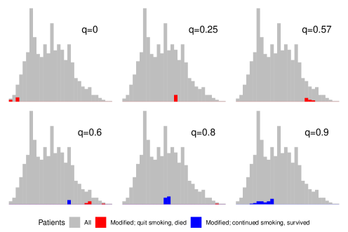
Figure 2: Histograms for the confounder, number of years smoked. The grey bins correspond to all cases in the study (min=1, max=64), and the colored bins correspond to cases selected to have their outcome modified by the generalized fragility index.

The remaining panes show the same for different values of $q$. As $q$ grows larger than $0$, the selected cases having increasingly higher years smoked since the cases with lower years smoked no longer have an outcome modification permitted. When $q=0.57$ the years smoked of the selected cases reaches the right tail in the distribution of all the cases. After, at $q=0.6$, cases who did not quit smoking and survived (in blue) begin to have their outcome modified. The years smoked of these selected cases is large. As $q$ grows further, the selected cases have lower years smoked. When $q=0.9$, the years smoked of the selected cases reaches the left tail of the distribution of all the cases.

Each example illustrates that the most atypical cases with permitted modifications will be selected for their outcome to be modified.

3.2.3 Stochastic generalized fragility indices

The stochastic fragility indices resolve this shortcoming by ensuring that outcome modifications of typical cases can reverse significance. Figure 3 visualizes the stochastic generalized fragility indices corresponding to the test controlling for the years smoking confounder. Notice that the stochastic generalized fragility index is monotonically decreasing in both $r$ and $q$.

When $q=0.9$ so that only very likely outcome modification are permitted, the generalized fragility index is $-30$ (indicated in red at the top of the figure). When the stochastic threshold $r$ grows beyond $0$ to $0.25,0.5,$ or $0.75$, the stochastic generalized fragility indices are much larger: they are $-1458$, $-1517$, and $-1569$, respectively. Therefore, for example, $1517$ cases must be selected to ensure that typical (i.e. more than half of) case collections can reverse significance with only very likely modifications (i.e. modifications which have likelihood at least $0.9$). In general the choices $r=0.25,0.5,$ and $0.75$ produce similar stochastic generalized fragility indices for each value of the sufficiently likely threshold $q$. Notice that these values are large because few cases have permitted outcome modifications which can contribute towards reversing significance when $q$ is large.

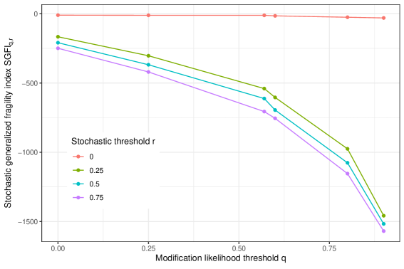
Figure 3: The stochastic generalized fragility indices for various choices of stochastic threshold $r$ and sufficiently likely threshold $q$.

4 Conclusion

We believe there is a promising future for statistics based on cases counts. They are broadly interpretable to medical researchers and others from varied backgrounds. The fragility index is an interesting addition to a statistician’s toolkit, in addition to the other fragility measures developed here.

The stochastic generalized fragility indices complete the foundational methodological development of the fragility index. Together with the sufficiently likely construction that permits only plausible modifications, they ensure that fragility measures are not driven by atypical cases and that the modifications are realistic. They study and improve both the case selection and the modification selection which defines fragility measures. Recall that the patients selected by a stochastic generalized fragility index were made to be typical by forcing a portion of the possible case collections to have permitted outcomes which can reverse significance.

Through the Bush v. Gore example we saw that the stochastic generalized fragility indices take into account the rarity of cases whose outcomes must be modified to reverse significance in the generalized fragility index. Next, through the adverse event example, we saw that the cases whose outcomes are modified in a generalized fragility index can be highly unusual relative to the remaining cases in a study when there are additional explanatory variables.

All fragility measures rely on choosing permitted outcome modifications which will have the largest impact on significance. Put differently, they all rely on an adversarial choice of the outcome modification (Lowd and Meek,, 2005). In view of Table 1, this is due to the “$\exists$” in each entry of the last row. Future work which introduces a new category of measures that deviates from this could be interesting and may bridge the gap between fragility measures and $p$ values. Randomly choosing outcome modifications may work for fragility indices with initially significant tests but not in general.

5 Acknowledgements

The authors gratefully thank Apurva Dixit and Derrick Tam for developing an early version of the stochastic fragility indices, alongside SEF.

References

- Ahmed et al., (2016) Ahmed, W., Fowler, R. A., and McCredie, V. A. (2016). Does sample size matter when interpreting the fragility index? Critical Care Medicine, 44(11):e1142–e1143.
- (2) Baer, B. R., Fremes, S. E., Charlson, M. E., Gaudino, M. F., and Wells, M. T. (2021a). Fragilitytools. https://github.com/brb225/FragilityTools. Accessed: 2021-1-12.
- (3) Baer, B. R., Gaudino, M., Charlson, M., Fremes, S. E., and Wells, M. T. (2021b). Fragility indices for only sufficiently likely modifications. Proceedings of the National Academy of Sciences, 118(49):e2105254118.
- (4) Baer, B. R., Gaudino, M., Fremes, S. E., Charlson, M., and Wells, M. T. (2021c). The fragility index can be used for sample size calculations. Journal of Clinical Epidemiology, 139(1):199–209.
- Benjamin and Berger, (2019) Benjamin, D. J. and Berger, J. O. (2019). Three recommendations for improving the use of p-values. The American Statistician, 73(S1):186–191.
- Benjamini et al., (2021) Benjamini, Y., De Veaux, R. D., Efron, B., Evans, S., Glickman, M., Graubard, B. I., He, X., Meng, X.-L., Reid, N. M., Stigler, S. M., et al. (2021). Asa president’s task force statement on statistical significance and replicability. CHANCE, 34(4):10–11.
- Berger and Sellke, (1987) Berger, J. O. and Sellke, T. (1987). Testing a point null hypothesis: The irreconcilability of p values and evidence. Journal of the American Statistical Association, 82(397):112–122.
- Blitzstein and Hwang, (2019) Blitzstein, J. K. and Hwang, J. (2019). Introduction to Probability. Chapman and Hall.
- Coakley and Hettmansperger, (1992) Coakley, C. W. and Hettmansperger, T. P. (1992). Breakdown bounds and expected test resistance. Journal of Nonparametric Statistics, 1(4):267–276.
- Coakley and Hettmansperger, (1994) Coakley, C. W. and Hettmansperger, T. P. (1994). The maximum resistance of tests. Australian Journal of Statistics, 36(2):225–233.
- Davies and Gather, (2005) Davies, P. L. and Gather, U. (2005). Breakdown and groups. The Annals of Statistics, 33(3):977–1035.
- Dixon, (1950) Dixon, R. G. (1950). Electoral college procedure. Western Political Quarterly, 3(2):214–224.
- Donoho and Huber, (1983) Donoho, D. L. and Huber, P. J. (1983). The notion of breakdown point. A Festschrift for Erich L. Lehmann, 1:157–184.
- Feinstein, (1990) Feinstein, A. R. (1990). The unit fragility index: an additional appraisal of “statistical significance” for a contrast of two proportions. Journal of Clinical Epidemiology, 43(2):201–209.
- Florida, (2000) Florida (2000). Florida department of state: Division of elections. https://results.elections.myflorida.com/Index.asp?ElectionDate=11/7/2000. Accessed: 2020-8-12.
- Frank et al., (2021) Frank, K. A., Lin, Q., Maroulis, S., Mueller, A. S., Xu, R., Rosenberg, J. M., Hayter, C. S., Mahmoud, R. A., Kolak, M., and Dietz, T. (2021). Hypothetical case replacement can be used to quantify the robustness of trial results. Journal of Clinical Epidemiology, 134(1):150–159.
- Goodman, (2008) Goodman, S. (2008). A dirty dozen: twelve p-value misconceptions. In Seminars in Hematology, volume 45, pages 135–140. Elsevier.
- Goodman, (1999) Goodman, S. N. (1999). Toward evidence-based medical statistics. 1: The p value fallacy. Annals of Internal Medicine, 130(12):995–1004.
- Greenland et al., (2016) Greenland, S., Senn, S. J., Rothman, K. J., Carlin, J. B., Poole, C., Goodman, S. N., and Altman, D. G. (2016). Statistical tests, p values, confidence intervals, and power: a guide to misinterpretations. European journal of Epidemiology, 31(4):337–350.
- Hampel, (1968) Hampel, F. R. (1968). Contributions to the theory of robust estimation. University of California, Berkeley.
- Hampel et al., (1986) Hampel, F. R., Ronchetti, E. M., Rousseeuw, P. J., and Stahel, W. A. (1986). Robust Statistics: the Approach Based on Influence Functions. John Wiley & Sons.
- Hernán and Robins, (2020) Hernán, M. A. and Robins, J. M. (2020). Causal Inference: What If. https://cdn1.sph.harvard.edu/wp-content/uploads/sites/1268/2021/03/ciwhatif_hernanrobins_30mar21.pdf. Accessed: 2020-8-12.
- Herrera-Perez et al., (2019) Herrera-Perez, D., Haslam, A., Crain, T., Gill, J., Livingston, C., Kaestner, V., Hayes, M., Morgan, D., Cifu, A. S., and Prasad, V. (2019). Meta-research: A comprehensive review of randomized clinical trials in three medical journals reveals 396 medical reversals. Elife, 8:e45183.
- Holek et al., (2020) Holek, M., Bdair, F., Khan, M., Walsh, M., Devereaux, P., Walter, S. D., Thabane, L., and Mbuagbaw, L. (2020). Fragility of clinical trials across research fields: A synthesis of methodological reviews. Contemporary Clinical Trials, 97:106151.
- Johnson et al., (2017) Johnson, K. W., Rappaport, E., Shameer, K., Glicksberg, B. S., and Dudley, J. T. (2017). fragilityindex: Fragility index for dichotomous and multivariate results. Unpublished package vignette.
- Jolliffe and Lukudu, (1993) Jolliffe, I. T. and Lukudu, S. G. (1993). The influence of a single observation on some standard test statistics. Journal of Applied Statistics, 20(1):143–151.
- Kafadar, (2021) Kafadar, K. (2021). Statistical significance, p-values, and replicability. The Annals of Applied Statistics, 15(3):1081–1083.
- Khan et al., (2020) Khan, M. S., Fonarow, G. C., Friede, T., Lateef, N., Khan, S. U., Anker, S. D., Harrell, F. E., and Butler, J. (2020). Application of the reverse fragility index to statistically nonsignificant randomized clinical trial results. JAMA Network Open, 3(8):e2012469.
- Lehmann and Romano, (2006) Lehmann, E. L. and Romano, J. P. (2006). Testing Statistical Hypotheses. Springer, New York.
- Lin, (2020) Lin, L. (2020). Factors that impact fragility index and their visualizations. Journal of Evaluation in Clinical Practice, 27(2):356–364.
- Lowd and Meek, (2005) Lowd, D. and Meek, C. (2005). Adversarial learning. In Proceedings of the Eleventh ACM SIGKDD, pages 641–647.
- Mayo, (2021) Mayo, D. G. (2021). The statistics wars and intellectual conflicts of interest.
- Polyak and Juditsky, (1992) Polyak, B. T. and Juditsky, A. B. (1992). Acceleration of stochastic approximation by averaging. SIAM Journal on Control and Optimization, 30(4):838–855.
- Poole, (1987) Poole, C. (1987). Confidence intervals exclude nothing. American Journal of Public Health, 77(4):492–493.
- Purdum, (2000) Purdum, T. S. (2000). Counting the vote: The overview; Bush is declared winner in Florida, but Gore vows to contest results. https://www.nytimes.com/2000/11/27/us/counting-vote-overview-bush-declared-winner-florida-but-gore-vows-contest.html. Accessed: 2020-8-12.
- Rieder, (1982) Rieder, H. (1982). Qualitative robustness of rank tests. The Annals of Statistics, 10(1):205–211.
- Ruppert, (1988) Ruppert, D. (1988). Efficient estimations from a slowly convergent Robbins-Monro process. Technical report, Cornell University.
- Simpson, (1989) Simpson, D. G. (1989). Hellinger deviance tests: efficiency, breakdown points, and examples. Journal of the American Statistical Association, 84(405):107–113.
- USSC, (2010) USSC (2010). Matrixx Initiatives, inc., et al. v. Siracusano et al. No. 09-1156.
- Walsh et al., (2014) Walsh, M., Srinathan, S. K., McAuley, D. F., Mrkobrada, M., Levine, O., Ribic, C., Molnar, A. O., Dattani, N. D., Burke, A., Guyatt, G., et al. (2014). The statistical significance of randomized controlled trial results is frequently fragile: a case for a fragility index. Journal of Clinical Epidemiology, 67(6):622–628.
- Wasserstein and Lazar, (2016) Wasserstein, R. L. and Lazar, N. A. (2016). The ASA statement on p-values: Context, process, and purpose. The American Statistician, 70(2):129–133.
- Ylvisaker, (1977) Ylvisaker, D. (1977). Test resistance. Journal of the American Statistical Association, 72(359):551–556.
- Zhang, (1996) Zhang, J. (1996). The sample breakdown points of tests. Journal of Statistical Planning and Inference, 52(2):161–181.