Difference-in-Differences for Continuous Treatments and Instruments with Stayers

Abstract

We propose difference-in-differences estimators for continuous treatments with heterogeneous effects. We assume that between consecutive periods, the treatment of some units, the switchers, changes, while the treatment of other units does not change. We show that under a parallel trends assumption, an unweighted and a weighted average of the slopes of switchers’ potential outcomes can be estimated. While the former parameter may be more intuitive, the latter can be used for cost-benefit analysis, and it can often be estimated more precisely. We generalize our estimators to the instrumental-variable case. We use our results to estimate the price-elasticity of gasoline consumption.

Keywords: differences-in-differences, continuous treatment, two-way fixed effects regressions, heterogeneous treatment effects, panel data, policy evaluation, instrumental variable.

JEL Codes: C21, C23

1 Introduction

A popular method to estimate the effect of a treatment on an outcome is to compare over time units experiencing different evolutions of their exposure to treatment. In practice, this idea is implemented by estimating regressions that control for unit and time fixed effects. de Chaisemartin and D’Haultfœuille (2023a) find that 26 of the 100 most cited papers published by the American Economic Review from 2015 to 2019 have used a two-way fixed effects (TWFE) regression to estimate the effect of a treatment on an outcome. de Chaisemartin and D’Haultfœuille (2020), Goodman-Bacon (2021), and Borusyak et al. (2021) have shown that under a parallel trends assumption, TWFE regressions are not robust to heterogeneous effects: they may estimate a weighted sum of treatment effects across periods and units, with some negative weights. Owing to the negative weights, the TWFE treatment coefficient could be, say, negative, even if the treatment effect is positive for every unit $\times$ period. Importantly, the result in de Chaisemartin and D’Haultfœuille (2020) applies to binary, discrete, and continuous treatments.

Several alternative heterogeneity-robust difference-in-difference (DID) estimators have been proposed (see Table 2 of de Chaisemartin and D’Haultfœuille, 2023b). Some apply to binary and staggered treatments (see Sun and Abraham, 2021; Callaway and Sant’Anna, 2021; Borusyak et al., 2021). Some apply to designs where all units start with a treatment equal to $0$, and then get treated with heterogeneous, potentially continuously distributed treatment intensities (see de Chaisemartin and D’Haultfœuille, 2023a; Callaway et al., 2021). By contrast, here we allow the treatment to be continuously distributed at every period, as may for instance be the case of trade tariffs (see Fajgelbaum et al., 2020) or gasoline taxes (see Li et al., 2014). Note that de Chaisemartin and D’Haultfœuille (2023a) extend our approach to models with dynamic effects (see Section 1.10 of their Web Appendix), while this paper focuses on models where past treatments do not affect the current outcome. Allowing for dynamic effects may be appealing, but in designs with continuous treatments, doing so may lead to hard-to-interpret and noisy estimators (see de Chaisemartin and D’Haultfœuille, 2023a).

We assume that we have a panel data set, whose units could be geographical locations such as counties. We start by considering the case where the panel has two time periods. From period one to two, the treatment of some units, hereafter referred to as the switchers, changes. On the other hand, the treatment of other units, hereafter referred to as the stayers, does not change. We propose a novel parallel trends assumption on the outcome evolution of switchers and stayers with the same period-one treatment, in the counterfactual where switchers’ treatment would not have changed. Under that assumption, we show that two target parameters can be estimated. Our first target is the average slope of switchers’ period-two potential outcome function, from their period-one to their period-two treatment, hereafter referred to as the Average Of Switchers’ Slopes (AOSS). Our second target is a weighted average of switchers’ slopes, where switchers receive a weight proportional to the absolute value of their treatment change, hereafter referred to as the Weighted Average Of Switchers’ Slopes (WAOSS).

Economically, our two parameters can serve different purposes, so neither parameter dominates the other. Under shape restrictions on the potential outcome function, we show that the AOSS can be used to infer the effect of other treatment changes than those that took place from period one to two. Instead, the WAOSS can be used to conduct a cost-benefit analysis of the treatment changes that effectively took place. On the other hand, when it comes to estimation, the WAOSS unambiguously dominates the AOSS. First, we show that it can be estimated at the standard parametric rate even if units can experience an arbitrarily small change of their treatment between consecutive periods. Second, we show that under some conditions, the asymptotic variance of the WAOSS estimator is strictly lower than that of the AOSS estimator. Third, unlike the AOSS, the WAOSS is amenable to doubly-robust estimation.

Then, we consider the instrumental-variable (IV) case. For instance, one may be interested in estimating the price-elasticity of a good’s consumption. If prices respond to demand shocks, the consumption trends of units experiencing and not experiencing a price change may not be parallel. On the other hand, the consumption trends of units experiencing and not experiencing a tax change may be parallel. Then, taxes may be used as an instrument for prices. In such cases, we show that the reduced-form WAOSS effect of the instrument on the outcome divided by the first-stage WAOSS effect is equal to a weighted average of the slopes of switchers’ outcome-slope with respect to the treatment, where switchers with a larger first-stage effect receive more weight. The ratio of the reduced-form and first-stage AOSS effects is also equal to a weighted average of slopes, with arguably less natural weights, so in the IV case the WAOSS seems both economically and statistically preferable to the AOSS.

We consider a few other extensions. First, we extend our results to applications with more than two time periods. Second, we propose a placebo estimator of the parallel trends assumption underlying our estimators. Third, we discuss how our estimators can be applied to discrete treatments taking a large number of values.

Finally, we use the yearly, 1966 to 2008 US state-level panel dataset of Li et al. (2014) to estimate the effect of gasoline taxes on gasoline consumption and prices. Using the WAOSS estimators, we find a significantly negative effect of taxes on gasoline consumption, and a significantly positive effect on prices. The AOSS estimators are close to, and not significantly different from, the WAOSS estimators, but they are also markedly less precise: their standard errors are almost three times larger than that of the WAOSS estimators. For gasoline consumption, the AOSS estimator is marginally significant, and for prices it is insignificant. Thus, even if one were interested in inferring the effect of other tax changes than those observed in the data, a policy question for which the AOSS is a more relevant target, a bias-variance trade-off may actually suggest using the WAOSS. We also compute an IV-WAOSS estimator of the price elasticity of gasoline consumption, and find a fairly small elasticity of -0.76, in line with previous literature (for instance, Hausman and Newey, 1995, find a long-run elasticity of -0.81). Our estimated elasticity is 30% smaller than, but not significantly different from, that obtained from a 2SLS TWFE regression. Our placebo estimators are small, insignificant, and fairly precisely estimated, thus suggesting that switchers and stayers may indeed be on parallel trends in this application.

Stata and R packages computing our estimators will be available soon. Some of our estimators can already be computed by the did_multiplegt Stata and R packages (see the earlier versions of this paper for details).

Related Literature.

On top of the aforementioned papers in the recent heterogeneity-robust DID literature, our paper builds upon several previous papers in the panel data literature. Chamberlain (1982) seems to be the first paper to have proposed an estimator of the AOSS parameter. Under the assumption of no counterfactual time trend, the estimator therein is a before-after estimator. Then, our paper is closely related to the work of Graham and Powell (2012), who also propose DID estimators of the AOSS when the treatment is continuously distributed at every time period. Their estimators rely on a linear treatment effect assumption (see their Equation (1)) and assume that units experience the same evolution of their treatment effect over time, a parallel-trends-on-treatment-effects assumption (see their Assumption 1.1(i) and (iii)). By contrast, our estimator of the AOSS does not place any restriction on treatment effects. But our main contribution to this literature is to introduce, and propose an estimator of, the WAOSS.

de Chaisemartin and D’Haultfœuille (2018) and de Chaisemartin and D’Haultfœuille (2020) also compare switchers and stayers with the same baseline treatment, to form heterogeneity-robust DID estimators of the effect of binary or discrete treatments. Those papers have shown that comparing switchers and stayers with the same period-one treatment is important: unconditional comparisons implicitly assume constant treatment effects over time, and are therefore not robust to time-varying effects. With a continuous treatment, the sample does not contain switchers and stayers with the exact same baseline treatment, so this paper’s contribution is to use non-parametric regression or propensity-score reweighting to compare switchers and stayers “with the exact same baseline treatment”.

D’Haultfœuille et al. (2023) also consider a DID-like estimator of the effect of a continuous treatment, but their estimator relies on a common change assumption akin to that in Athey and Imbens (2006), rather than on a parallel trends assumption.

Finally, our estimators require that there be some stayers, whose treatment does not change between consecutive time periods. This assumption is unlikely to be met when the treatment is say, precipitations: for instance, US counties never experience the exact same amount of precipitations over two consecutive years. In de Chaisemartin et al. (2023), we discuss the (non-trivial) extension of the results in this paper to applications without stayers.

Organization of the paper.

In Section 2, we present the set-up, introduce notation and discuss our main assumptions. In Section 3, we introduce the AOSS and discuss its identification and estimation. Section 4 then turns to the WAOSS. Section 5 extends our previous results to an instrumental variable set-up. We consider other extensions in Section 6. Finally, our application is developed in Section 7. The proofs are collected in the appendix.

2 Set-up and assumptions

A representative unit is drawn from an infinite super population, and observed at two time periods. This unit could be an individual or a firm, but it could also be a geographical unit, like a county or a region. All expectations below are taken with respect to the distribution of variables in the super population. We are interested in the effect of a continuous and scalar treatment variable on that unit’s outcome. Let $D_{1}$ (resp. $D_{2}$) denote the unit’s treatment at period 1 (resp. 2), and let $\mathcal{D}_{1}$ (resp. $\mathcal{D}_{2}$) be the set of values $D_{1}$ (resp. $D_{2}$) can take, i.e. its support. For any $d\in\mathcal{D}_{1}\cup\mathcal{D}_{2}$, let $Y_{1}(d)$ and $Y_{2}(d)$ respectively denote the unit’s potential outcomes at periods 1 and 2 with treatment $d$. Finally, let $Y_{1}$ and $Y_{2}$ denote their observed outcomes at periods 1 and 2. Let $S=1\{D_{2}\neq D_{1}\}$ be an indicator equal to 1 if the unit’s treatment changes from period one to two, i.e. if they are a switcher.

In what follows, all equalities and inequalities involving random variables are required to hold almost surely. For any random variables observed at the two time periods $(X_{1},X_{2})$, let $\Delta X=X_{2}-X_{1}$ denote the change of $X$ from period $1$ to $2$.

We make the following assumptions.

Assumption 1

(Parallel trends) For all $d\in\mathcal{D}_{1}$, $E(\Delta Y(d)|D_{1}=d,D_{2})=E(\Delta Y(d)|D_{1}=d)$.

Assumption 1 is a parallel trends assumption. It requires that $\Delta Y(d)$ be mean independent of $D_{2}$, conditional on $D_{1}=d$. It has one key implication we leverage for identification: the counterfactual outcome evolution switchers would have experienced if their treatment had not changed is identified by the outcome evolution of stayers with the same period-one treatment:

$$E(\Delta Y(d)|D_{1}=d,S=1)=E(\Delta Y(d)|D_{1}=d,S=0).$$ (1)

Accordingly, the DID estimators we propose below compare switchers and stayers with the same period-one treatment.

Instead, one could propose DID estimators comparing switchers and stayers, without conditioning on their period-one treatment. On top of Assumption 1, such estimators rest on two supplementary conditions:

1. $E(\Delta Y(d)|D_{1}=d)=E(\Delta Y(d))$.

2. For all $(d,d^{\prime})\in\mathcal{D}_{1}^{2}$, $E(\Delta Y(d))=E(\Delta Y(d^{\prime}))$.

(i) requires that all units experience the same evolution of their potential outcome with treatment $d$, while Assumption 1 only imposes that requirement for units with the same baseline treatment. Assumption 1 may be more plausible: units with the same period-one treatment may be more similar and more likely to be on parallel trends than units with different period-one treatments. (ii) requires that the trend affecting all potential outcomes be the same. Rearranging, (ii) is equivalent to assuming

$$E(Y_{2}(d)-Y_{2}(d^{\prime}))=E(Y_{1}(d)-Y_{1}(d^{\prime})):$$ (2)

the treatment effect should be constant over time, a strong restriction on treatment effect heterogeneity. Assumption 1, on the other hand, does not impose any restriction on treatment effect heterogeneity, as it only restricts one potential outcome per unit.

Assumption 2

(Bounded treatment, Lipschitz and bounded potential outcomes)

1. $\mathcal{D}_{1}$ and $\mathcal{D}_{2}$ are bounded subsets of $\mathbb{R}$.

2. For all $t\in\{1,2\}$ and for all $(d,d^{\prime})\in\mathcal{D}_{t}^{2}$, there is a random variable $\overline{Y}\geq 0$ such that $|Y_{t}(d)-Y_{t}(d^{\prime})|\leq\overline{Y}|d-d^{\prime}|$, with $\sup_{(d_{1},d_{2})\in\text{Supp}(D_{1},D_{2})}E[\overline{Y}|D_{1}=d_{1},D_{2}=d_{2}]<\infty$.

Assumption 2 is a technical condition ensuring that all the expectations below are well defined. It requires that the set of values that the period-one and period-two treatments can take be bounded. It also requires that the potential outcome functions be Lipschitz (with an individual specific Lipschitz constant). This will automatically hold if $d\mapsto Y_{2}(d)$ is differentiable with respect to $d$ and has a bounded derivative.

For estimation and inference, we assume we observe an iid sample with the same distribution as $(Y_{1},Y_{2},D_{1},D_{2})$:

Assumption 3

(iid sample) We observe $(Y_{i,1},Y_{i,2},D_{i,1},D_{i,2})_{1\leq i\leq n}$, that are independent and identically distributed vectors with the same probability distribution as $(Y_{1},Y_{2},D_{1},D_{2})$.

Importantly, Assumption 3 allows for the possibility that $Y_{1}$ and $Y_{2}$ (resp. $D_{1}$ and $D_{2}$) are serially correlated, as is commonly assumed in DID studies (see Bertrand et al., 2004).

3 Estimating the average of switchers’ slopes

3.1 Target parameter

In this section, our target parameter is

$$\delta_{1} :=E\left(\frac{Y_{2}(D_{2})-Y_{2}(D_{1})}{D_{2}-D_{1}}\middle|S=1\right).$$ (3)

$\delta_{1}$ is the average, across switchers, of the effect on their period-two outcome of moving their treatment from its period-one to its period-two value, scaled by the difference between these two values. In other words, $\delta_{1}$ is the average of the slopes of switchers’ potential outcome functions, between their period-one and their period-two treatments. Hereafter, $\delta_{1}$ is referred to as the Average Of Switchers’ Slopes (AOSS). Note that with a binary treatment such that all units are untreated at period 1 and some units get treated at period 2, the AOSS reduces to the standard average treatment effect on the treated. Thus, the AOSS generalizes that parameter to non-binary treatments and more complicated designs.

The AOSS averages effects of discrete rather than infinitesimal changes in the treatment as in Hoderlein and White (2012), for instance. But if one slightly reinforces Point 2 of Assumption 2 by supposing that $d\mapsto Y_{2}(d)$ is differentiable on $\mathcal{D}_{1}\cup\mathcal{D}_{2}$, by the mean value theorem,

$$\frac{Y_{2}(D_{2})-Y_{2}(D_{1})}{D_{2}-D_{1}}=Y^{\prime}_{2}\left(\tilde{D}\right)$$

for some $\tilde{D}\in(\min(D_{1},D_{2}),\max(D_{1},D_{2}))$. Then, the AOSS is an average marginal effect on switchers:

$$\delta_{1}=E[Y^{\prime}_{2}\left(\tilde{D}\right)|S=1].$$ (4)

The only difference with the usual average marginal effect on switchers $E[Y^{\prime}_{2}(D_{2})|S=1]$ is that the derivative is evaluated at $\tilde{D}$ instead of $D_{2}$. Note that (4) implies that unlike TWFE regression coefficients, the AOSS satisfies the no-sign reversal property. If $Y^{\prime}_{2}(d)\geq 0$ for all $d$, meaning that increasing the treatment always increases the outcome of every switcher, $\delta_{1}\geq 0$.

However, the AOSS is a local effect. First, it only applies to switchers. Second, it measures the effect of changing their treatment from its period-one to its period-two value, not of other changes of their treatment. Still, the AOSS can be used to identify the effect of other treatment changes under shape restrictions on the potential outcome function. First, assume that the potential outcomes are linear: for $t\in\{1,2\}$,

$$Y_{t}(d)=Y_{t}(0)+B_{t}d,$$

where $B_{t}$ is a slope that may vary across units and may change over time. Then, $\delta_{1}=E\left(B_{2}\middle|S=1\right)$: the AOSS is equal to the average, across switchers, of the slopes of their potential outcome functions at period 2. Therefore, for all $d\neq d^{\prime}$,

$$E(Y_{2}(d)-Y_{2}(d^{\prime})|S=1)=(d-d^{\prime})\delta_{1}:$$

under linearity, knowing the AOSS is sufficient to recover the ATE of any uniform treatment change among switchers. Of course, this only holds under linearity, which may not be a plausible assumption. Assume instead that $d\mapsto Y_{2}(d)$ is convex. Then, for any $\epsilon>0$,

$$E\left(Y_{2}(D_{2}+\epsilon)-Y_{2}(D_{1})\middle|S=1\right)\geq E\left(Y_{2}(D_{2})-Y_{2}(D_{1})\middle|S=1\right)+\epsilon\delta_{1}.$$

$E\left(Y_{2}(D_{2})-Y_{2}(D_{1})\middle|S=1\right)$ can be identified following the same steps as those we use to identify the AOSS below. Accordingly, under convexity one can use the AOSS to obtain a lower bound of the effect of changing the treatment from $D_{1}$ to a larger value than $D_{2}$. For instance, in Fajgelbaum et al. (2020), one can use this strategy to derive a lower bound of the effect of even larger tariffs’ increases than those implemented by the Trump administration. Under convexity, one can also derive an upper bound of the effect of changing the treatment from $D_{1}$ to a lower value than $D_{2}$. And under concavity, one can derive an upper (resp. lower) bound of the effect of changing the treatment from $D_{1}$ to a larger (resp. lower) value than $D_{2}$. Importantly, the AOSS is identified even if those linearity or convexity/concavity conditions fail. But those conditions are necessary to use the AOSS to identify or bound the effects of alternative policies.

3.2 Identification

To identify the AOSS, we use a DID estimand comparing switchers and stayers with the same period-one treatment. This requires that there be no value of the period-one treatment $D_{1}$ such that only switchers have that value, as stated formally below.

Assumption 4

(Support condition for AOSS identification) $P(S=1)>0$, $P(S=1|D_{1})<1$.

Assumption 4 implies that $P(S=0)>0$, meaning that there are stayers whose treatment does not change. While we assume that $D_{1}$ and $D_{2}$ are continuous, we also assume that the treatment is persistent, and thus $\Delta D$ has a mixed distribution with a mass point at zero.

To identify the AOSS, we also start by assuming that there are no quasi-stayers: the treatment of all switchers changes by at last $c$ from period one to two, for some strictly positive $c$.

Assumption 5

(No quasi-stayers) $\exists c>0$: $P(|\Delta D|>c|S=1)=1$.

We relax Assumption 5 just below.

Theorem 1

If Assumptions 1-5 hold,

$$\delta_{1} =E\left(\frac{\Delta Y-E(\Delta Y|D_{1},S=0)}{\Delta D}\middle|S=1\right).$$

Intuitively, the effect of changing a switcher’s treatment from its period-one to its period-two value is identified by a DID comparing its outcome evolution to that of stayers with the same period-one treatment. Then, this DID is normalized by $\Delta D$, to recover the slope of the switcher’s potential outcome function.

If there are quasi-stayers, the AOSS is still identified. For any $\eta>0$, let $S_{\eta}=1\{|\Delta D|>\eta\}$ be an indicator equal to one for switchers whose treatment changes by at least $\eta$ from period one to two.

Theorem 2

If Assumptions 1-4 hold,

$$\delta_{1} =\lim_{\eta\downarrow 0}E\left(\frac{\Delta Y-E(\Delta Y|D_{1},S=0)}{\Delta D}\middle|S_{\eta}=1\right).$$

If there are quasi-stayers whose treatment change is arbitrarily close to $0$ (i.e. $f_{|\Delta D||S=1}(0)>0$), the denominator of $(\Delta Y-E(\Delta Y|D_{1},S=0))/\Delta D$ is very close to $0$ for them. On the other hand,

$$\Delta Y-E(\Delta Y|D_{1},S=0)$$

$$= Y_{2}(D_{2})-Y_{2}(D_{1})+\Delta Y(D_{1})-E(\Delta Y(D_{1})|D_{1},S=0)$$

$$\approx \Delta Y(D_{1})-E(\Delta Y(D_{1})|D_{1},S=0),$$

so the ratio’s numerator may not be close to $0$. Then, under weak conditions,

$$E\left(\left|\frac{\Delta Y-E(\Delta Y|D_{1},S=0)}{\Delta D}\right|\;\middle|S=1\right)=+\infty.$$

Therefore, we need to trim quasi-stayers from the estimand in Theorem 1, and let the trimming go to 0 to still recover $\delta_{1}$, as in Graham and Powell (2012) who consider a related estimand with some quasi-stayers. Accordingly, while the AOSS is still identified with quasi-stayers, it is irregularly identified by a limiting estimand.

3.3 Estimation and inference

With no quasi-stayers, $E\left((\Delta Y-E(\Delta Y|D_{1},S=0))/\Delta D\middle|S=1\right)$ can be estimated in three steps. First, one estimates $E(\Delta Y|D_{1},S=0)$ using a non-parametric regression of $\Delta Y_{i}$ on $D_{i,1}$ among stayers. Second, for each switcher, one computes $\widehat{E}(\Delta Y|D_{1}=D_{i,1},S=0)$, its predicted outcome evolution given its baseline treatment, according to the non-parametric regression estimated among stayers. Third, one lets

$$\widehat{\delta}_{1}:= \frac{1}{n_{s}}\sum_{i:S_{i}=1}\frac{\Delta Y_{i}-\widehat{E}(\Delta Y|D_{1}=D_{i,1},S=0)}{\Delta D_{i}},$$

where $n_{s}=\#\{i:S_{i}=1\}$.

To estimate $E(\Delta Y|D_{1},S=0)$, we consider a series estimator based on polynomials in $D_{1}$, $(p_{k,K_{n}}(D_{1}))_{1\leq k\leq K_{n}}$. We make the following technical assumption.

Assumption 6

(Conditions for asymptotic normality of AOSS estimator)

1. $D_{1}$ is continuously distributed on a compact interval $I$, with $\inf_{d\in I}f_{D_{1}}(d)>0$.

2. $E[\Delta Y^{2}]<\infty$ and $d\mapsto E[\Delta Y^{2}|D_{1}=d]$ is bounded on $I$.

3. $P(S=1)>0$ and $\sup_{d\in I}P(S=1|D_{1}=d)<1$.

4. The functions $d\mapsto E[(1-S)\Delta Y|D_{1}=d]$, $d\mapsto E[S|D_{1}=d]$ and $d\mapsto E[S/\Delta D|D_{1}=d]$ are four times continuously differentiable.

5. The polynomials $d\mapsto p_{k,K_{n}}(d)$, $1\leq k\leq K_{n}$, are orthonormal on $I$ and $K_{n}^{12}/n\to+\infty$, $K_{n}^{7}/n\to 0$.

Point 3 is a slight reinforcement of Assumption 4. In Point 5, $K_{n}^{12}/n\to\infty$ requires that $K_{n}$, the order of the polynomial in $D_{1}$ we use to approximate $E(\Delta Y|D_{1},S=0)$, goes to $+\infty$ when the sample size grows, thus ensuring that the bias of our series estimator of $E(\Delta Y|D_{1},S=0)$ tends to zero. $K_{n}^{7}/n\to 0$ ensures that $K_{n}$ does not go to infinity too fast, thus preventing overfitting.

Theorem 3

If Assumptions 1-3 and 5-6 hold,

$$\sqrt{n}\left(\widehat{\delta}_{1}-\delta_{1}\right)\stackrel{{\scriptstyle d}}{{\longrightarrow}}\mathcal{N}(0,V(\psi_{1})),$$

where

$$\psi_{1} :=\frac{1}{E(S)}\left\{\left(\frac{S}{\Delta D}-E\left(\left.\frac{S}{\Delta D}\right|D_{1}\right)\frac{(1-S)}{E[1-S|D_{1}]}\right)[\Delta Y-E(\Delta Y|D_{1},S=0)]-\delta_{1}S\right\}.$$

Theorem 3 shows that without quasi-stayers, the AOSS can be estimated at the $\sqrt{n}-$rate, and gives an expression of its estimator’s asymptotic variance. With quasi-stayers, we conjecture that the AOSS cannot be estimated at the $\sqrt{n}-$rate. This conjecture is based on a result from Graham and Powell (2012). Though their result applies to a broader class of estimands, it implies in particular that with quasi-stayers,

$$\lim_{\eta\downarrow 0}E\left(\frac{\Delta Y-E(\Delta Y|S=0)}{\Delta D}\middle|S_{\eta}=1\right)$$

cannot be estimated at a faster rate than $n^{1/3}$. The estimand in the previous display is closely related to our estimand

$$\lim_{\eta\downarrow 0}E\left(\frac{\Delta Y-E(\Delta Y|D_{1},S=0)}{\Delta D}\middle|S_{\eta}=1\right)$$

in Theorem 2, and is equal to it if $E(\Delta Y|D_{1},S=0)=E(\Delta Y|S=0)$. Then, even though the assumptions in Graham and Powell (2012) differ from ours, it seems reasonable to assume that their general conclusion still applies to our set-up: here as well, owing to $\delta_{1}$’s irregular identification, this parameter can probably not be estimated at the parametric $\sqrt{n}-$rate with quasi-stayers. This is one of the reasons that lead us to consider, in the next section, another target parameter that can be estimated at the parametric $\sqrt{n}-$rate with quasi-stayers.

4 Estimating a weighted average of switchers’ slopes

4.1 Target parameter

In this section, our target parameter is

$$\delta_{2}:= E\left(\frac{|D_{2}-D_{1}|}{E(|D_{2}-D_{1}||S=1)}\times\frac{Y_{2}(D_{2})-Y_{2}(D_{1})}{D_{2}-D_{1}}\middle|S=1\right)$$

$$= \frac{E\left(\text{sgn}(D_{2}-D_{1})(Y_{2}(D_{2})-Y_{2}(D_{1}))\middle|S=1\right)}{E(|D_{2}-D_{1}||S=1)}$$

$$= \frac{E\left(\text{sgn}(D_{2}-D_{1})(Y_{2}(D_{2})-Y_{2}(D_{1}))\right)}{E(|D_{2}-D_{1}|)}.$$

$\delta_{2}$ is a weighted average of the slopes of switchers’ potential outcome functions from their period-one to their period-two treatments, where slopes receive a weight proportional to switchers’ absolute treatment change from period one to two. Accordingly, we refer to $\delta_{2}$ as the Weighted Average Of Switchers’ Slopes (WAOSS). All slopes are weighted positively, so the WAOSS satisfies the no-sign reversal property, like the AOSS.

It is easy to see that $\delta_{2}=\delta_{1}$ if and only if

$$\text{cov}\left(\frac{Y_{2}(D_{2})-Y_{2}(D_{1})}{D_{2}-D_{1}},|D_{2}-D_{1}|\middle|S=1\right)=0:$$ (5)

the WAOSS and AOSS are equal if and only if switchers’ slopes are uncorrelated with $|D_{2}-D_{1}|$.

Economically, the AOSS and WAOSS serve different purposes. As discussed above, under shape restrictions on the potential outcome function, the AOSS can be used to identify or bound the effect of other treatment changes than the actual change switchers experienced from period one to two. The WAOSS cannot serve that purpose, but under some assumptions, it may be used to conduct a cost-benefit analysis of the treatment changes that took place from period one to two. To simplify the discussion, let us assume in the remainder of this paragraph that $D_{2}\geq D_{1}$. Assume also that the outcome is a measure of output, such as agricultural yields or wages, expressed in monetary units. Finally, assume that the treatment is costly, with a cost linear in dose, uniform across units, and known to the analyst: the cost of giving $d$ units of treatment to a unit at period $t$ is $c_{t}\times d$ for some known $(c_{t})_{t\in\{1,2\}}$. Then, $D_{2}$ is beneficial relative to $D_{1}$ if and only if $E(Y_{2}(D_{2})-c_{2}D_{2})>E(Y_{2}(D_{1})-c_{2}D_{1})$ or, equivalently,

$$\delta_{2}>c_{2}.$$

Then, comparing $\delta_{2}$ to the per-unit treatment cost is sufficient to evaluate if changing the treatment from $D_{1}$ to $D_{2}$ was beneficial.

4.2 Identification

Let $S_{+}=1\{D_{2}-D_{1}>0\}$, $S_{-}=1\{D_{2}-D_{1}<0\}$ and

$$\delta_{2+} :=\frac{E\left(Y_{2}(D_{2})-Y_{2}(D_{1})|S_{+}=1\right)}{E(D_{2}-D_{1}|S_{+}=1)},$$

$$\delta_{2-} :=\frac{E\left(Y_{2}(D_{1})-Y_{2}(D_{2})|S_{-}=1\right)}{E(D_{1}-D_{2}|S_{-}=1)}.$$

Hereafter, units with $S_{+}=1$ are referred to as “switchers up”, while units with $S_{-}=1$ are referred to as “switchers down”. Thus, $\delta_{2+}$ is the WAOSS of switchers up, and $\delta_{2-}$ is the WAOSS of switchers down. One has

$$\delta_{2}= \frac{P(S_{+}=1|S=1)E(D_{2}-D_{1}|S_{+}=1)}{E(|D_{2}-D_{1}||S=1)}\delta_{2+}$$

$$+ \frac{P(S_{-}=1|S=1)E(D_{1}-D_{2}|S_{-}=1)}{E(|D_{2}-D_{1}||S=1)}\delta_{2-}.$$ (6)

To identify $\delta_{2+}$ (resp. $\delta_{2-}$) we use DID estimands comparing switchers up (resp. switchers down) to stayers with the same period-one treatment. This requires that there be no value of $D_{1}$ such that some switchers up (resp. switchers down) have that baseline treatment while there is no stayer with the same baseline treatment, as stated in Point 1 (resp. 2) of Assumption 7 below.

Assumption 7

(Support conditions for WAOSS identification)

1. $0<P(S_{+}=1)$, and $0<P(S_{+}=1|D_{1})$ implies that $0<P(S=0|D_{1})$.

2. $0<P(S_{-}=1)$, and $0<P(S_{-}=1|D_{1})$ implies that $0<P(S=0|D_{1})$.

Theorem 4

1. If Assumptions 1-2 and Point 1 of Assumption 7 hold,

   $$\delta_{2+} =\frac{E\left(\Delta Y-E(\Delta Y|D_{1},S=0)\middle|S_{+}=1\right)}{E(\Delta D|S_{+}=1)}$$ (7)

   $$=\frac{E\left(\Delta Y|S_{+}=1\right)-E\left(\Delta Y\frac{P(S_{+}=1|D_{1})}{P(S=0|D_{1})}\frac{P(S=0)}{P(S_{+}=1)}\middle|S=0\right)}{E(\Delta D|S_{+}=1)}.$$ (8)

2. If Assumptions 1-2 and Point 2 of Assumption 7 hold,

   $$\delta_{2-} =\frac{E\left(\Delta Y-E(\Delta Y|D_{1},S=0)\middle|S_{-}=1\right)}{E(\Delta D|S_{-}=1)}$$ (9)

   $$=\frac{E\left(\Delta Y|S_{-}=1\right)-E\left(\Delta Y\frac{P(S_{-}=1|D_{1})}{P(S=0|D_{1})}\frac{P(S=0)}{P(S_{-}=1)}\middle|S=0\right)}{E(\Delta D|S_{-}=1)}.$$ (10)

3. If Assumptions 1-2 and Assumption 7 hold,

   $$\delta_{2}= \frac{E\left[\text{sgn}(\Delta D)\left(\Delta Y-E(\Delta Y|D_{1},S=0)\right)\right]}{E[|\Delta D|]}$$ (11)

   $$= \frac{E\left[\text{sgn}(\Delta D)\Delta Y\right]-E\left[\Delta Y\frac{P(S_{+}=1|D_{1})-P(S_{-}=1|D_{1})}{P(S=0|D_{1})}P(S=0)\middle|S=0\right]}{E[|\Delta D|]}.$$ (12)

Point 1 of Theorem 4 shows that $\delta_{2+}$, the WAOSS of switchers-up, is identified by two estimands, a regression-based and a propensity-score-based estimand. Point 2 of Theorem 4 shows that $\delta_{2-}$, the WAOSS of switchers down, is identified by two estimands similar to those identifying $\delta_{2+}$, replacing $S_{+}$ by $S_{-}$. Finally, if the conditions in Point 1 and 2 of Theorem 4 jointly hold, it directly follows from (4.2) that $\delta_{2}$, the WAOSS of all switchers, is identified by a weighted average of the estimands in Equations (7) and (9), and by a weighted average of the estimands in Equations (8) and (10). Those weighted averages simplify into the expressions given in Point 3 of Theorem 4. Point 3 of Theorem 4 also implies that $\delta_{2}$ is identified by the following doubly-robust estimand:

$$\frac{E\left[\left(S_{+}-S_{-}-\frac{P(S_{+}=1|D_{1})-P(S_{-}=1|D_{1})}{P(S=0|D_{1})}(1-S)\right)(\Delta Y-E(\Delta Y|D_{1},S=0))\right]}{E[\left|\Delta D\right|]}.$$ (13)

4.3 Estimation and inference

The regression-based estimands identifying $\delta_{2+}$ and $\delta_{2-}$ can be estimated following almost the same steps as in Section 3.3. Specifically, let

$$\widehat{\delta}^{r}_{2+}:= \frac{\frac{1}{n_{+}}\sum_{i:S_{i+}=1}\left(\Delta Y_{i}-\widehat{E}(\Delta Y|D_{1}=D_{i,1},S=0)\right)}{\frac{1}{n_{+}}\sum_{i:S_{i+}=1}\Delta D_{i}}$$

$$\widehat{\delta}^{r}_{2-}:= \frac{\frac{1}{n_{-}}\sum_{i:S_{i-}=1}\left(\Delta Y_{i}-\widehat{E}(\Delta Y|D_{1}=D_{i,1},S=0)\right)}{\frac{1}{n_{-}}\sum_{i:S_{i-}=1}\Delta D_{i}},$$

where $n_{+}=\#\{i:S_{i+}=1\}$ and $n_{-}=\#\{i:S_{i-}=1\}$, and where $\widehat{E}(\Delta Y|D_{1},S=0)$ is the series estimator of $E(\Delta Y|D_{1},S=0)$ defined in Section 3.3 of the paper. Then, let

$$\widehat{w}_{+}=\frac{\frac{n_{+}}{n}\times\frac{1}{n_{+}}\sum_{i:S_{i+}=1}\Delta D_{i}}{\frac{n_{+}}{n}\times\frac{1}{n_{+}}\sum_{i:S_{i+}=1}\Delta D_{i}-\frac{n_{-}}{n}\times\frac{1}{n_{-}}\sum_{i:S_{i-}=1}\Delta D_{i}},$$

and let

$$\widehat{\delta}^{r}_{2}= \widehat{w}_{+}\widehat{\delta}^{r}_{2+}+(1-\widehat{w}_{+})\widehat{\delta}^{r}_{2-}$$

be the corresponding estimator of $\delta_{2}$.

We now propose estimators of the propensity-score-based estimands identifying $\delta_{2+}$ and $\delta_{2-}$ in Equations (8) and (10). Let $\widehat{P}(S_{+}=1)=n_{+}/n$ (resp. $\widehat{P}(S_{-}=1)=n_{-}/n$, $\widehat{P}(S=0)=(n-n_{s})/n$) be an estimator of $P(S_{+}=1)$ (resp. $P(S_{-}=1)$, $P(S=0)$). Let $\widehat{P}(S_{+}=1|D_{1})$ (resp. $\widehat{P}(S_{-}=1|D_{1})$, $\widehat{P}(S=0|D_{1})$) be a non-parametric estimator of $P(S_{+}=1|D_{1})$ (resp. $P(S_{-}=1|D_{1})$, $P(S=0|D_{1})$) using a series logistic regression of $S_{i+}$ (resp. $S_{i-}$, $1-S_{i}$) on polynomials in $D_{1}$ $(p_{k,K_{n}}(D_{1}))_{1\leq k\leq K_{n}}$. We make the following technical assumption.

Assumption 8

(Technical conditions for asymptotic normality of propensity-score WAOSS estimator)

1. $D_{1}$ is continuously distributed on a compact interval $I$, with $\inf_{d\in I}f_{D_{1}}(d)>0$.

2. $E[\Delta Y^{2}]<\infty$ and $d\mapsto E[\Delta Y^{2}|D_{1}=d]$ is bounded on $I$

3. $0<E[S_{+}]<1$, $0<E[S_{-}]<1$, $E[S]>0$ and $\sup_{d\in I}E[S|D_{1}=d]<1$.

4. The functions $d\mapsto E[\Delta Y(1-S)|D_{1}=d]$, $d\mapsto E[S|D_{1}=d]$, $d\mapsto E[S_{+}|D_{1}=d]$ and $d\mapsto E[S_{-}|D_{1}=d]$ are four times continuously differentiable.

5. The polynomials $d\mapsto p_{k,K_{n}}(d)$, $k\leq 1\leq K_{n}$ are orthonormal on $I$ and $K_{n}=Cn^{\nu}$ where $1/10<\nu<1/6$.

Let

$$\widehat{\delta}^{ps}_{2+}:= \frac{\frac{1}{n_{+}}\sum_{i:S_{i+}=1}\Delta Y_{i}-\frac{1}{n-n_{s}}\sum_{i:S_{i}=0}\Delta Y_{i}\frac{\widehat{P}(S_{+}=1|D_{1}=D_{i1})}{\widehat{P}(S=0|D_{1}=D_{i1})}\frac{\widehat{P}(S=0)}{\widehat{P}(S_{+}=1)}}{\frac{1}{n_{+}}\sum_{i:S_{i+}=1}\Delta D_{i}}$$

$$\widehat{\delta}^{ps}_{2-}:= \frac{\frac{1}{n_{-}}\sum_{i:S_{i-}=1}\Delta Y_{i}-\frac{1}{n-n_{s}}\sum_{i:S_{i}=0}\Delta Y_{i}\frac{\widehat{P}(S_{-}=1|D_{1}=D_{i1})}{\widehat{P}(S=0|D_{1}=D_{i1})}\frac{\widehat{P}(S=0)}{\widehat{P}(S_{-}=1)}}{\frac{1}{n_{-}}\sum_{i:S_{i-}=1}\Delta D_{i}},$$

and let

$$\widehat{\delta}^{ps}_{2}= \widehat{w}_{+}\widehat{\delta}^{ps}_{2+}+(1-\widehat{w}_{+})\widehat{\delta}^{ps}_{2-}$$

be the corresponding estimator of $\delta_{2}$. Let

$$\psi_{2+} :=\frac{1}{E(\Delta DS_{+})}\left\{\left(S_{+}-E(S_{+}|D_{1})\frac{(1-S)}{E(1-S|D_{1})}\right)(\Delta Y-E(\Delta Y|D_{1},S=0))-\delta_{2+}\Delta DS_{+}\right\}$$

$$\psi_{2-} :=\frac{1}{E(\Delta DS_{-})}\left\{\left(S_{-}-E(S_{-}|D_{1})\frac{(1-S)}{E(1-S|D_{1})}\right)(\Delta Y-E(\Delta Y|D_{1},S=0))-\delta_{2-}\Delta DS_{-}\right\}$$

$$\psi_{2} :=\frac{1}{E(\left|\Delta D\right|)}\left\{\left(S_{+}-S_{-}-E(S_{+}-S_{-}|D_{1})\frac{(1-S)}{E(1-S|D_{1})}\right)\right.$$

$$\qquad\times(\Delta Y-E(\Delta Y|D_{1},S=0))-\delta_{2}\left|\Delta D\right|\bigg{\}}.$$

Theorem 5

1. If Assumptions 1-3 and 6 hold,

   $$\sqrt{n}\left((\widehat{\delta}^{r}_{2+},\widehat{\delta}^{r}_{2-})^{\prime}-(\delta_{2+},\delta_{2-})^{\prime}\right)\stackrel{{\scriptstyle d}}{{\longrightarrow}}\mathcal{N}(0,V((\psi_{2+},\psi_{2-})^{\prime})).$$

   and

   $$\sqrt{n}\left(\widehat{\delta}^{r}_{2}-\delta_{2}\right)\stackrel{{\scriptstyle d}}{{\longrightarrow}}\mathcal{N}(0,V(\psi_{2})).$$

2. If Assumptions 1-3 and 8 hold,

   $$\sqrt{n}\left((\widehat{\delta}^{ps}_{2+},\widehat{\delta}^{ps}_{2-})^{\prime}-(\delta_{2+},\delta_{2-})^{\prime}\right)\stackrel{{\scriptstyle d}}{{\longrightarrow}}\mathcal{N}(0,V((\psi_{2+},\psi_{2-})^{\prime})).$$

   and

   $$\sqrt{n}\left(\widehat{\delta}^{ps}_{2}-\delta_{2}\right)\stackrel{{\scriptstyle d}}{{\longrightarrow}}\mathcal{N}(0,V(\psi_{2})).$$

Based on (13), we can also estimate $\delta_{2}$ using the following doubly-robust estimator:

$$\hat{\delta}^{dr}_{2}=\frac{\sum_{i}\left(S_{i+}-S_{i-}-\frac{\hat{P}(S_{+}=1|D_{1}=D_{1i})-P(S_{i-}=1|D_{1}=D_{1i})}{P(S_{i}=0|D_{1}=D_{1i})}(1-S_{i})\right)(\Delta Y_{i}-\hat{E}(\Delta Y_{i}|D_{1}=D_{1i},S_{i}=0))}{\sum_{i}\left|\Delta D_{i}\right|}.$$

Finally, we now show that under some assumptions, the asymptotic variance of the WAOSS estimator is lower than that of the AOSS estimator. While the assumptions under which this result is obtained are admittedly strong, this still suggests that one may often expect an efficiency gain from using the WAOSS.

Proposition 1

If Assumption 1 holds, $(Y_{2}(D_{2})-Y_{2}(D_{1}))/(D_{2}-D_{1})=\delta$ for some real number $\delta$, $V(\Delta Y(D_{1})|D_{1},D_{2})=\sigma^{2}$ for some real number $\sigma^{2}$, $D_{2}\geq D_{1}$, and $\Delta D\perp\!\!\!\perp D_{1}$, then

$$V(\psi_{1})= \sigma^{2}\left[\frac{E(1/(\Delta D)^{2}|S=1)}{P(S=1)}+\frac{\left(E(1/\Delta D|S=1)\right)^{2}}{P(S=0)}\right]$$

$$\geq \sigma^{2}\frac{1}{\left(E(\Delta D|S=1)\right)^{2}}\left[\frac{1}{P(S=1)}+\frac{1}{P(S=0)}\right]=V(\psi_{2}),$$

with equality if and only if $V(\Delta D|S=1)=0$.

5 Instrumental-variable estimation

There are instances where the parallel-trends condition in Assumption 1 is implausible, but one has at hand an instrument satisfying a similar parallel-trends condition. For instance, one may be interested in estimating the price-elasticity of a good’s consumption, but prices respond to supply and demand shocks, and therefore do not satisfy Assumption 1. On the other hand, taxes may not respond to supply and demand shocks and may satisfy a parallel-trends assumption.

5.1 Notation and assumptions

Let $(Z_{1},Z_{2})$ denote the instrument’s values at period one and two and $\mathcal{Z}_{t}$ be the support of $Z_{t}$. For any $z\in\mathcal{Z}_{1}\cup\mathcal{Z}_{2}$, let $D_{1}(z)$ and $D_{2}(z)$ respectively denote the unit’s potential treatments at periods 1 and 2 with instrument $z$. Let $SC=1\{D_{2}(Z_{2})\neq D_{2}(Z_{1})\}$ be an indicator equal to 1 for switchers-compliers, namely units whose instrument changes from period one to two and whose treatment is affected by that change in the instrument. We make the following assumptions.

Assumption 9

(Reduced-form and first-stage parallel trends) For all $z\in\mathcal{Z}_{1}$,

1. $E(\Delta Y(D_{1}(z))|Z_{1}=z,Z_{2})=E(\Delta Y(D_{1}(z))|Z_{1}=z)$.

2. $E(\Delta D_{1}(z)|Z_{1}=z,Z_{2})=E(\Delta D_{1}(z)|Z_{1}=z)$.

Point 1 of Assumption 9 requires that $\Delta Y(D_{1}(z))$, units’ outcome evolutions in the counterfactual where their instrument does not change from period one to two, be mean independent of $Z_{2}$, conditional on $Z_{1}$. Point 2 requires that units’ treatment evolutions under $Z_{1}$ be mean independent of $Z_{2}$, conditional on $Z_{1}$. de Chaisemartin (2010) and Hudson et al. (2017) consider IV-DID estimands and also introduce “reduced-form” and “first-stage” parallel trends assumptions.

Assumption 10

(Monotonicity) For all $(z,z^{\prime})\in\mathcal{Z}_{2}^{2}$, $z\geq z^{\prime}\Rightarrow D_{2}(z)\geq D_{2}(z^{\prime})$.

Assumption 10 is a monotonicity assumption similar to that in Imbens and Angrist (1994). It requires that increasing the period-two instrument weakly increases the period-two treatment.

Assumption 11

(Bounded instrument, Lipschitz and bounded reduced-form potential outcomes and potential treatments)

1. $\mathcal{Z}_{1}$ and $\mathcal{Z}_{2}$ are bounded subsets of $\mathbb{R}$.

2. For all $t\in\{1,2\}$ and for all $(z,z^{\prime})\in\mathcal{Z}_{t}^{2}$, there is a random variable $\overline{Y}\geq 0$ such that $|Y_{t}(D_{t}(z))-Y_{t}(D_{t}(z^{\prime}))|\leq\overline{Y}|z-z^{\prime}|$, with $\sup_{(z_{1},z_{2})\in\text{Supp}(Z_{1},Z_{2})}E[\overline{Y}|Z_{1}=z_{1},Z_{2}=z_{2}]<\infty$.

3. For all $t\in\{1,2\}$ and for all $(z,z^{\prime})\in\mathcal{Z}_{t}^{2}$, there is a random variable $\overline{D}\geq 0$ such that $|D_{t}(z)-D_{t}(z^{\prime})|\leq\overline{D}|z-z^{\prime}|$, with $\sup_{(z_{1},z_{2})\in\text{Supp}(Z_{1},Z_{2})}E[\overline{D}|Z_{1}=z_{1},Z_{2}=z_{2}]<\infty$.

Assumption 11 is an adaptation of Assumption 2 to the IV setting we consider in this section.

Assumption 12

(iid sample) We observe $(Y_{i,1},Y_{i,2},D_{i,1},D_{i,2},Z_{i,1},Z_{i,2})_{1\leq i\leq n}$, that are independent and identically distributed with the same probability distribution as $(Y_{1},Y_{2},D_{1},D_{2},Z_{1},Z_{2})$.

5.2 Target parameter

In this section, our target parameter is

$$\delta_{IV}:= E\left(\frac{|D_{2}(Z_{2})-D_{2}(Z_{1})|}{E(|D_{2}(Z_{2})-D_{2}(Z_{1})||SC=1)}\times\frac{Y_{2}(D_{2}(Z_{2}))-Y_{2}(D_{2}(Z_{1}))}{D_{2}(Z_{2})-D_{2}(Z_{1})}\middle|SC=1\right).$$

$\delta_{IV}$ is a weighted average of the slopes of compliers-switchers’ period-two potential outcome functions, from their period-two treatment under their period-one instrument, to their period-two treatment under their period-two instrument. Slopes receive a weight proportional to the absolute value of compliers-switchers’ treatment response to the instrument change. $\delta_{IV}$ is just equal to the reduced-form WAOSS effect of the instrument on the outcome, divided by the first-stage WAOSS effect of the instrument on the treatment. Hereafter, we refer to $\delta_{IV}$ as the IV-WAOSS. We could also consider a reduced-form AOSS divided by a first-stage AOSS. The resulting target parameter is a weighted average of the slopes $\frac{Y_{2}(D_{2}(Z_{2}))-Y_{2}(D_{2}(Z_{1}))}{D_{2}(Z_{2})-D_{2}(Z_{1})}$, with weights proportional to $\frac{D_{2}(Z_{2})-D_{2}(Z_{1})}{Z_{2}-Z_{1}}$. It may be more natural to weight compliers-switchers’ slopes by the absolute value of their first-stage response than by the slope of their first-stage response.

5.3 Identification

Let $S^{I}=1\{Z_{2}-Z_{1}\neq 0\}$, $S^{I}_{+}=1\{Z_{2}-Z_{1}>0\}$, and $S^{I}_{-}=1\{Z_{2}-Z_{1}<0\}$.

Assumption 13

(Support conditions for IV-WAOSS identification)

1. $0<P(S^{I}_{+}=1)$, and $0<P(S^{I}_{+}=1|Z_{1})$ implies that $0<P(S^{I}=0|Z_{1})$.

2. $0<P(S^{I}_{-}=1)$, and $0<P(S^{I}_{-}=1|Z_{1})$ implies that $0<P(S^{I}=0|Z_{1})$.

Theorem 6

If Assumptions 9-11 and 13 hold,

$$\delta_{IV}= \frac{E\left[\text{sgn}(\Delta Z)\left(\Delta Y-E(\Delta Y|Z_{1},S^{I}=0)\right)\right]}{E\left[\text{sgn}(\Delta Z)\left(\Delta D-E(\Delta D|Z_{1},S^{I}=0)\right)\right]}$$ (14)

$$= \frac{E\left[\text{sgn}(\Delta Z)\Delta Y\right]-E\left[\Delta Y\frac{P(S^{I}_{+}=1|Z_{1})-P(S^{I}_{-}=1|Z_{1})}{P(S^{I}=0|Z_{1})}P(S^{I}=0)\middle|S^{I}=0\right]}{E\left[\text{sgn}(\Delta Z)\Delta D\right]-E\left[\Delta D\frac{P(S^{I}_{+}=1|Z_{1})-P(S^{I}_{-}=1|Z_{1})}{P(S^{I}=0|Z_{1})}P(S^{I}=0)\middle|S^{I}=0\right]}.$$ (15)

The regression-based (resp. propensity-score-based) estimand identifying $\delta_{IV}$ is just equal to the regression-based (resp. propensity-score-based) estimand identifying the reduced-form WAOSS effect of the instrument on the outcome, divided by the regression-based (resp. propensity-score-based) estimand identifying the first-stage WAOSS effect.

5.4 Estimation and inference

Let

$$\widehat{\delta}^{r}_{IV}= \frac{\frac{1}{n}\sum_{i=1}^{n}\text{sgn}(\Delta Z_{i})\left(\Delta Y_{i}-\widehat{E}(\Delta Y|Z_{1}=Z_{i,1},S^{I}=0)\right)}{\frac{1}{n}\sum_{i=1}^{n}\text{sgn}(\Delta Z_{i})\left(\Delta D_{i}-\widehat{E}(\Delta D|Z_{1}=Z_{i,1},S^{I}=0)\right)},$$ (16)

where $\widehat{E}(\Delta Y|Z_{1},S^{I}=0)$ and $\widehat{E}(\Delta D|Z_{1},S^{I}=0)$ are series estimators of $E(\Delta Y|Z_{1},S^{I}=0)$ and $E(\Delta D|Z_{1},S^{I}=0)$ defined analogously to the series estimator in Section 3.3.

Let $n^{I}_{s}=\#\{i:S^{I}_{i}=1\}$, and let

$$\widehat{\delta}^{ps}_{IV}= \frac{\frac{1}{n}\sum_{i=1}^{n}\text{sgn}(\Delta Z_{i})\Delta Y_{i}-\frac{1}{n-n^{I}_{s}}\sum_{i:S^{I}_{i}=0}\Delta Y_{i}\frac{\widehat{P}(S^{I}_{+}=1|Z_{1}=Z_{i1})-\widehat{P}(S^{I}_{-}=1|Z_{1}=Z_{i1})}{\widehat{P}(S^{I}=0|Z_{1}=Z_{i1})}\widehat{P}(S^{I}=0)}{\frac{1}{n}\sum_{i=1}^{n}\text{sgn}(\Delta Z_{i})\Delta D_{i}-\frac{1}{n-n^{I}_{s}}\sum_{i:S^{I}_{i}=0}\Delta D_{i}\frac{\widehat{P}(S^{I}_{+}=1|Z_{1}=Z_{i1})-\widehat{P}(S^{I}_{-}=1|Z_{1}=Z_{i1})}{\widehat{P}(S^{I}=0|Z_{1}=Z_{i1})}\widehat{P}(S^{I}=0)},$$ (17)

where $\widehat{P}(S^{I}=0)=(n-n^{I}_{s})/n$, and $\widehat{P}(S^{I}_{+}=1|Z_{1})$ (resp. $\widehat{P}(S^{I}_{-}=1|Z_{1})$, $\widehat{P}(S^{I}=0|Z_{1})$) is a series logistic regression estimator of $P(S^{I}_{+}=1|Z_{1})$ (resp. $P(S^{I}_{-}=1|Z_{1})$, $P(S^{I}=0|Z_{1})$) defined analogously to the series logistic regression estimators in Section 4.3.

For any variable $X$, let

$$\delta_{X} =E\left[\text{sgn}(\Delta Z)\left(\Delta X-E(\Delta X|Z_{1},S^{I}=0)\right)\right]$$

$$\psi_{X} =\frac{1}{E(\left|\Delta Z\right|)}\left\{\left(S^{I}_{+}-S^{I}_{-}-E(S^{I}_{+}-S^{I}_{-}|Z_{1})\frac{(1-S^{I})}{E(1-S^{I}|Z_{1})}\right)\right.$$

$$\qquad\times(\Delta X-E(\Delta X|D_{1},S^{I}=0))-\delta_{X}\left|\Delta Z\right|\bigg{\}}.$$

Then, let

$$\psi_{IV} =\frac{\psi_{Y}-\delta_{IV}\psi_{D}}{\delta_{D}}.$$

Under technical conditions similar to those in Assumptions 6 and 8, one can show that

$$\sqrt{n}\left(\widehat{\delta}^{r}_{IV}-\delta_{IV}\right)\stackrel{{\scriptstyle d}}{{\longrightarrow}}\mathcal{N}(0,V(\psi_{IV})),$$

$$\sqrt{n}\left(\widehat{\delta}^{ps}_{IV}-\delta_{IV}\right)\stackrel{{\scriptstyle d}}{{\longrightarrow}}\mathcal{N}(0,V(\psi_{IV})).$$

6 Extensions

In this section, we return to the case where the treatment, rather than an instrument, satisfies a parallel-trends condition. Combining the extensions below with the IV case is possible.

6.1 Discrete treatments

While in this paper we focus on continuous treatments, our results can also be applied to discrete treatments. In Section 4 of their Web Appendix, de Chaisemartin and D’Haultfœuille (2020) already propose a DID estimator of the effect of a discrete treatment. The plug-in estimator of $\delta_{2}$ one can form following Theorem 4 and using simple averages to estimate the non-parametric regressions or the propensity scores is numerically equivalent to the estimator therein. This paper still makes two contributions relative to de Chaisemartin and D’Haultfœuille (2020) when the treatment is discrete. First, the estimator based on Theorem 1 was not proposed therein. Second, with a discrete treatment taking a large number of values, the estimator in de Chaisemartin and D’Haultfœuille (2020) may not be applicable as it requires finding switchers and stayers with the exact same period-one treatment, which may not always be feasible. Instead, one can use the estimators proposed in this paper.

6.2 More than two time periods

In this section, we assume the representative unit is observed at $T>2$ time periods. Let $(D_{1},...,D_{T})$ denote the unit’s treatments and $\mathcal{D}_{t}=\text{Supp}(D_{t})$ for all $t\in\{1,...,T\}$. For any $t\in\{1,...,T\}$, and for any $d\in\mathcal{D}_{t}$ let $Y_{t}(d)$ denote the unit’s potential outcome at period $t$ with treatment $d$. Finally, let $Y_{t}$ denote their observed outcome at $t$. For any $t\in\{2,...,T\}$, let $S_{t}=1\{D_{t}\neq D_{t-1}\}$ be an indicator equal to 1 if the unit’s treatment switches from period $t-1$ to $t$. Let also $S_{+,t}=1\{D_{t}>D_{t-1}\}$ and $S_{-,t}=1\{D_{t}<D_{t-1}\}$. We assume that the assumptions made in the paper, rather than just holding for $t=1$ and $t=2$, actually hold for all pairs of consecutive time periods $(t-1,t)$. For instance, we replace Assumption 1 by:

Assumption 14

(Parallel trends) For all $t\geq 2$, for all $d\in\mathcal{D}_{t-1}$, $E(\Delta Y_{t}(d)|D_{t-1}=d,D_{t})=E(\Delta Y_{t}(d)|D_{t-1}=d)$.

To preserve space, we do not restate our other assumptions with more than two periods.

Let

$$\delta_{1,t} =E\left(\frac{Y_{t}(D_{t})-Y_{t}(D_{t-1})}{D_{t}-D_{t-1}}\middle|S_{t}=1\right),$$

$$\delta_{2,t} =\frac{E\left(\text{sgn}(D_{t}-D_{t-1})(Y_{t}(D_{t})-Y_{t}(D_{t-1}))\right)}{E(|D_{t}-D_{t-1}|)}.$$

Let

$$\delta^{T\geq 3}_{1} =\sum_{t=2}^{T}\frac{P(S_{t}=1)}{\sum_{k=2}^{T}P(S_{k}=1)}\delta_{1,t},$$

$$\delta^{T\geq 3}_{2} =\sum_{t=2}^{T}\frac{E(|\Delta D_{t}|)}{\sum_{k=2}^{T}E(|\Delta D_{k}|)}\delta_{2,t}$$

be generalizations of the AOSS and WAOSS effects to applications with more than two periods. Note that in line with the spirit of the two effects, we propose different weights to aggregate the AOSS and WAOSS across time periods. For the AOSS, the weights are just proportional to the proportion of switchers between $t-1$ and $t$. For the WAOSS, the weights are proportional to the average absolute value of the treatment switch from $t-1$ to $t$.

Theorem 7

If Assumption 14 and generalizations of Assumptions 2-5 to more than two periods hold,

$$\delta^{T\geq 3}_{1}= \sum_{t=2}^{T}\frac{P(S_{t}=1)}{\sum_{k=2}^{T}P(S_{k}=1)}E\left(\frac{\Delta Y_{t}-E(\Delta Y_{t}|D_{t-1},S_{t}=0)}{\Delta D_{t}}\middle|S_{t}=1\right).$$

Theorem 8

If Assumption 14 and generalizations of Assumptions 2 and 7 to more than two periods hold,

$$\delta^{T\geq 3}_{2}= \sum_{t=2}^{T}\frac{E(|\Delta D_{t}|)}{\sum_{k=2}^{T}E(|\Delta D_{k}|)}\frac{E\left(\text{sgn}(\Delta D_{t})\left(\Delta Y_{t}-E(\Delta Y_{t}|D_{t-1},S_{t}=0)\right)\right)}{E(|\Delta D_{t}|)}$$

$$= \sum_{t=2}^{T}\frac{E(|\Delta D_{t}|)}{\sum_{k=2}^{T}E(|\Delta D_{k}|)}\frac{E\left[\text{sgn}(\Delta D_{t})\Delta Y_{t}\right]-E\left[\Delta Y_{t}\frac{P(S_{+,t}=1|D_{t-1})-P(S_{-,t}=1|D_{t-1})}{P(S_{t}=0|D_{t-1})}P(S_{t}=0)\middle|S_{t}=0\right]}{E(|\Delta D_{t}|)}.$$

Theorems 7 and 8 are straightforward generalizations of Theorems 1 and 4 to settings with more than two time periods.

Let

$$\psi^{num}_{1,t}= \left(\frac{S_{t}}{\Delta D_{t}}-E\left(\frac{S_{t}}{\Delta D_{t}}\middle|D_{t-1}\right)\frac{(1-S_{t})}{E[1-S_{t}|D_{t-1}]}\right)[\Delta Y_{t}-E(\Delta Y_{t}|D_{t-1},S_{t}=0)]-\delta_{1,t}P(S_{t}=1),$$

$$\psi^{num}_{2,t}= \left(S_{+,t}-S_{-,t}-E(S_{+,t}-S_{-,t}|D_{t-1})\frac{(1-S_{t})}{E(1-S_{t}|D_{t-1})}\right)(\Delta Y_{t}-E(\Delta Y_{t}|D_{t-1},S_{t}=0))-\delta_{2,t}E(|\Delta D_{t}|).$$

After some algebra, one can show that the influence function of the AOSS estimator with is several periods is

$$\psi^{T\geq 3}_{1} :=\frac{\sum_{t=2}^{T}\psi^{num}_{1,t}-\delta^{T\geq 3}_{1}\sum_{t=2}^{T}S_{t}}{\sum_{t=2}^{T}P(S_{t})},$$ (18)

while the influence function of the WAOSS estimators with several periods is

$$\psi^{T\geq 3}_{2} :=\frac{\sum_{t=2}^{T}\psi^{num}_{2,t}-\delta^{T\geq 3}_{2}\sum_{t=2}^{T}|\Delta D_{t}|}{\sum_{t=2}^{T}E(|\Delta D_{t}|)}.$$ (19)

Importantly, those influence functions allow the unit’s treatments and outcomes to be arbitrarily serially correlated.

6.3 Testing for pre-trends

With several time periods, one can test the following condition, which is closely related to Assumption 14:

Assumption 15

(Testable parallel trends) For all $t\geq 2,t\leq T-1$, for all $d\in\mathcal{D}_{t-1}$, $E(\Delta Y_{t}(d)|D_{t-1}=d,D_{t},D_{t+1})=E(\Delta Y_{t}(d)|D_{t-1}=d)$.

To test that condition, one can compute a placebo version of the estimators described in the previous subsection, replacing $\Delta Y_{t}$ by $\Delta Y_{t-1}$, and restricting the sample, for each pair of consecutive time periods $(t-1,t)$, to units whose treatment did not change between $t-2$ and $t-1$. Thus, the placebo compares the average $\Delta Y_{t-1}$ of the $t-1$-to-$t$ switchers and stayers, restricting attention to $t-2$-to-$t-1$ stayers.

7 Application

Data and research questions.

We use the yearly 1966-to-2008 panel dataset of Li et al. (2014), covering 48 US states (Alaska and Hawaii are excluded). For each state$\times$year cell $(g,t)$, the data contains $Z_{g,t}$, the total (state plus federal) gasoline tax in cents per gallon, $D_{g,t}$, the log tax-inclusive price of gasoline, and $Y_{g,t}$, the log gasoline consumption per adult. Our goal is to estimate the effect of gasoline taxes on gasoline consumption and prices, and to estimate the price-elasticity of gasoline consumption, using taxes as an instrument. Instead, Li et al. (2014) jointly estimate the effect of gasoline taxes and tax-exclusive prices on consumption, using a TWFE regression with two treatments. Between each pair of consecutive periods, the tax-exclusive price changes in all states, so this treatment does not have stayers and its effect cannot be estimated using the estimators proposed in this paper. Thus, our estimates cannot be compared to those of Li et al. (2014).

Switching cells, and how they compare to the entire sample.

Let $\mathcal{S}$ be the set of switching $(g,t)$ cells such that $Z_{g,t}\neq Z_{g,t-1}$ but $Z_{g^{\prime},t}=Z_{g^{\prime},t-1}$ for some $g^{\prime}$. The second condition drops from the estimation seven pairs of consecutive time periods between which the federal gasoline tax changed, thus implying that all states experienced a change of their tax. $\mathcal{S}$ includes 384 cells, so effects of taxes on gasoline prices and consumptions can be estimated for 19% of the 2,016 state$\times$year cells for which $Z_{g,t}-Z_{g,t-1}$ can be computed. Table 1 below compares some observable characteristics of switchers and stayers. Switchers seem slightly over-represented in the later years of the panel: $t$ is on average 2.5 years larger for switchers than for stayers, and the difference is significant. On the other hand, switchers are not more populated than stayers, and their gasoline consumption and gasoline price in 1966 are not significantly different from that of stayers. Thus, there is no strong indication that the cells in $\mathcal{S}$ are a very selected subgroup.

Table 1: Comparing switchers and stayers

Dependent Variables:	$t$	Adult Population	log(quantity)1966	log(price)1966
Constant	1,986.7	3,691,608.0	-0.5161	3.471
	(0.2739)	(577,164.0)	(0.0210)	(0.0054)
$\mathbf{1}\{Z_{g,t}\neq Z_{g,t-1}\}$	2.481	39,588.0	-0.0099	0.0014
	(0.7519)	(320,342.1)	(0.0096)	(0.0029)
N	2,016	2,016	2,016	2,016

Notes: The table show the results of regressions of some dependent variables on a constant and an indicator for switching cells. The standard errors shown in parentheses are clustered at the state level.

Distribution of taxes.

As an example, the top panel of Figure 1 below shows the distribution of $Z_{g,1987}$ for 1987-to-1988 stayers, while the bottom panel shows the distribution for 1987-to-1988 switchers. The figure shows that there are many values of $Z_{g,1987}$ such that only one or two states have that value, so $Z_{g,1987}$ is close to being continuously distributed. Moreover, all switchers $g$ are such that

$$\min_{g^{\prime}:Z_{g^{\prime},1988}=Z_{g^{\prime},1987}}Z_{g^{\prime},1987}\leq Z_{g,1987}\leq\max_{g^{\prime}:Z_{g^{\prime},1988}=Z_{g^{\prime},1988}}Z_{g^{\prime},1987}.$$

Thus, Assumption 4 seems to hold for this pair of years. $(1987,1988)$ is not atypical. While $Z_{g,t}$ varies less across states in the first years of the panel, there are many other years where $Z_{g,t}$ is close to being continuously distributed. Similarly, almost 95% of cells in $\mathcal{S}$ are such that $\min_{g^{\prime}:Z_{g^{\prime},t}=Z_{g^{\prime},t-1}}Z_{g^{\prime},t-1}\leq Z_{g,t-1}\leq\max_{g^{\prime}:Z_{g^{\prime},t}=Z_{g^{\prime},t-1}}Z_{g^{\prime},t-1}$. Dropping the few cells that do not satisfy this condition barely changes the results presented below.

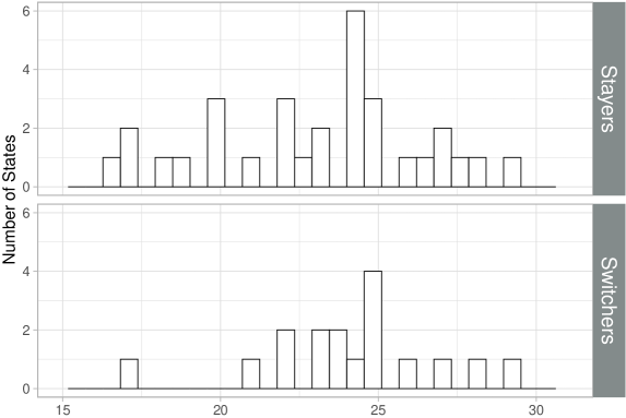
Figure 1: Gasoline tax in 1987 among 1987-to-1988 switchers and stayers

Distribution of tax changes.

Figure 2 below shows the distribution of $Z_{g,t}-Z_{g,t-1}$ for the 384 cells in $\mathcal{S}$. The majority experience an increase in their taxes, but 38 cells experience a decrease. The average value of $|Z_{g,t}-Z_{g,t-1}|$ is equal to 1.61 cents, while prior to the tax change, switchers’ average gasoline price is equal to 112 cents: our estimators leverage small changes in taxes relative to gasoline prices. Finally, $\min_{(g,t)\in\mathcal{S}}|Z_{g,t}-Z_{g,t-1}|=0.05$ : some switchers experience a very small change in their taxes. Their slope receives a weight equal to 1/384 in the AOSS estimators, and a weight 32.2 ($1.61/0.05$) times smaller in the WAOSS estimators.

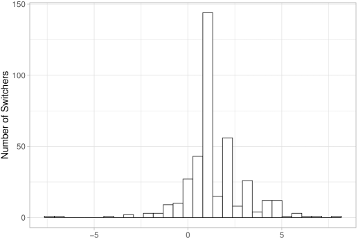
Figure 2: Distribution of tax changes between consecutive periods

Reduced-form and first-stage AOSS and WAOSS estimates.

Columns (1) and (3) of Table 2 below show the AOSS and doubly-robust WAOSS estimates of the reduced-form and first-stage effects of taxes on quantities and prices. First, the estimators are computed using a polynomial of order 1 in $D_{t-1}$ to estimate $E(\Delta Y_{t}|D_{t-1},S_{t}=0)$ and the propensity scores $P(S_{+,t}=1|D_{t-1})$, $P(S_{-,t}=1|D_{t-1})$, and $P(S_{t}=0|D_{t-1})$. Second, as a robustness check, the estimators are computed using a polynomial of order 2 in those estimations. With 48 states, and only 20 to 30 stayers for many pairs of consecutive time periods, fitting higher order polynomials could lead to overfitting. Columns (2) and (4) show standard errors clustered at the state level, computed following (18) and (19). Column (5) shows the p-value of a test that the AOSS and WAOSS effects are equal. All estimations use 1632 (48$\times$ 35) first-difference observations: 7 periods have to be excluded as they do not have stayers. In Panel A, the AOSS estimates indicate that increasing gasoline tax by 1 cent decreases quantities consumed by 0.5-0.6 percent on average for the switchers. That effect is significant at the 5% level when one uses linear models to estimate the aforementioned conditional expectations, and at the 10% level when one uses quadratic models. The WAOSS estimates are slightly lower than, but close to, the AOSS estimates. As predicted by Proposition 1, the standard errors of the WAOSS estimators are almost 3 times smaller than that of the AOSS estimators. Equality tests that the AOSS and WAOSS effects are equal are not rejected, thus suggesting that (5) may hold in this application. At least, the correlation between switchers’ tax changes and their slopes is not large enough to generate a detectable difference between the two parameters. In Panel B, the AOSS estimates of the first-stage effect are insignificant. The WAOSS estimates are significant, and they indicate that if gasoline tax increases by 1 cent on average, prices increase by around 0.5 percent on average for the switchers. Again, the differences between the AOSS and WAOSS effects of taxes on prices are insignificant.

Table 2: Effects of gasoline tax on quantities consumed and prices

Panel A: Reduced-form effect of taxes on quantities consumed.
	AOSS	s.e	WAOSS	s.e.	p-value	N
	(1)	(2)	(3)	(4)	(5)	(6)
log(quantity) - Linear model	-0.0058	0.0026	-0.0039	0.0009	0.357	1632
log(quantity) - Quadratic model	-0.0050	0.0026	-0.0038	0.0010	0.573	1632
Panel B: First-stage effect of taxes on quantities consumed.
	AOSS	s.e	WAOSS	s.e	p-value	N
log(price) - Linear model	0.0028	0.0023	0.0054	0.0009	0.154	1632
log(price) - Quadratic model	0.0024	0.0024	0.0050	0.0009	0.182	1632

Notes: All estimators in the table are computed using the data of Li et al. (2014). Columns (1) and (3) show the AOSS and doubly-robust WAOSS estimates of the reduced-form and first-stage effects of taxes on quantities and prices. First, the estimators are computed using a polynomial of order 1 in $D_{t-1}$ to estimate $E(\Delta Y_{t}|D_{t-1},S_{t}=0)$ and the propensity scores $P(S_{+,t}=1|D_{t-1})$, $P(S_{-,t}=1|D_{t-1})$, and $P(S_{t}=0|D_{t-1})$. Second, the estimators are computed using a polynomial of order 2 in those estimations. Columns (2) and (4) show estimated standard errors clustered at the state level and following (18) and (19). Column (5) shows the p-value of a test that the AOSS and WAOSS effects are equal.

Placebo analysis.

Table 3 below shows placebo AOSS and doubly-robust WAOSS estimates of the reduced-form and first-stage effects. The placebo estimators are analogous to the actual estimators, but they replace $\Delta Y_{t}$ by $\Delta Y_{t-1}$, and they restrict the sample, for each pair of consecutive time periods $(t-1,t)$, to states whose taxes did not change between $t-2$ and $t-1$. The placebo WAOSS estimates are small and insignificant, both for quantities and prices. Those placebos are fairly precisely estimated, and their confidence intervals do not contain the actual WAOSS estimates. The placebo AOSS estimates are larger for quantities, but they are insignificant, and less precisely estimated. This placebo analysis shows that before switchers change their gasoline taxes, switchers’ and stayers’ consumption of gasoline and gasoline prices do not follow detectably different evolutions.

Table 3: Placebo effects of gasoline tax on quantities consumed and prices

Panel A: Reduced-form placebo effect of taxes on quantities consumed.
	AOSS	s.e	WAOSS	s.e	N
	(1)	(2)	(3)	(4)	(5)
log(quantity) - Linear model	0.0038	0.0023	-0.0001	0.0011	1059
log(quantity) - Quadratic model	0.0039	0.0026	-0.0003	0.0011	1059
Panel B: First-stage placebo effect of taxes on prices.
	AOSS	s.e	WAOSS	s.e	N
	(1)	(2)	(3)	(4)	(5)
log(price) - Linear model	-0.0008	0.0047	0.0015	0.0013	1059
log(price) - Quadratic model	-0.0011	0.0045	0.0011	0.0013	1059

Notes: The table shows the placebo AOSS and doubly-robust WAOSS estimates of the reduced-form and first-stage effects of taxes on quantities and prices. The estimators and their standard errors are computed as the actual estimators, replacing $\Delta Y_{t}$ by $\Delta Y_{t-1}$, and restricting the sample, for each pair of consecutive time periods $(t-1,t)$, to states whose taxes did not change between $t-2$ and $t-1$.

IV-WAOSS estimate of the price-elasticity of gasoline consumption.

The first two lines of Table 4 show doubly-robust IV-WAOSS estimates of the price-elasticity of gasoline consumption. The third line shows a 2SLS-TWFE estimator, computed via a 2SLS regression of $Y_{g,t}$ on $D_{g,t}$ and state and year fixed effects, using $Z_{g,t}$ as the instrument. As the instrument’s first stage is not very strong and the sample effectively only has 48 observations, asymptotic approximations may not be reliable for inference. In line with that conjecture, we find that the bootstrap distributions of the three estimators in Table 4 are non-normal, with some very large outliers. Therefore, we use percentile bootstrap for inference, clustering the bootstrap at the state level. Reassuringly, these confidence intervals have nominal coverage in simulations taylored to our application. The IV-WAOSS estimates are negative, significant, and larger than -1, though their confidence intervals contain -1. The 2SLS-TWFE is 42% larger in absolute value, though Column (3) of the table shows that the IV-WAOSS and 2SLS-TWFE estimators do not significantly differ. Interestingly, the confidence interval attached to the 2SLS-TWFE estimator is about 27% wider than that of the IV-WAOSS estimators, thus showing that using a more robust estimator does not always come with a precision cost.

Table 4: IV estimators of the price-elasticity of gasoline consumption

	Estimator	95% CI	P-value	N
	(1)	(2)	(3)	(4)
IV-WAOSS - Linear Model	-0.726	[-1.349,-0.328]	0.358	1632
IV-WAOSS - Quadratic Model	-0.761	[-1.566,-0.068]	0.394	1632
2SLS-TWFE	-1.084	[-2.015,-0.502]		1632

Notes: The table shows the doubly-robust IV-WAOSS and 2SLS-TWFE estimates of the price-elasticity of gasoline consumption, computed using the data of Li et al. (2014). Percentile bootstrap confidence intervals are shown in Column (2). They are computed with 500 bootstrap replications, clustered at the state level. The p-value of an equality test of the IV-WAOSS and 2SLS-TWFE estimators, also computed by percentile bootstrap, is shown in Column (3).

8 Conclusion

We propose new difference-in-difference (DID) estimators for continuous treatments. We assume that between pairs of consecutive periods, the treatment of some units, the switchers, changes, while the treatment of other units, the stayers, does not change. We propose a parallel trends assumption on the outcome evolution of switchers and stayers with the same baseline treatment. Under that assumption, two target parameters can be estimated. Our first target is the average slope of switchers’ period-two potential outcome function, from their period-one to their period-two treatment, referred to as the AOSS. Our second target is a weighted average of switchers’ slopes, where switchers receive a weight proportional to the absolute value of their treatment change, referred to as the WAOSS. Economically, the AOSS and WAOSS serve different purposes, so neither parameter dominates the other. On the other hand, when it comes to estimation, the WAOSS unambiguously dominates the AOSS. First, it can be estimated at the parametric rate even if units can experience an arbitrarily small treatment change. Second, under some conditions, its asymptotic variance is strictly lower than that of the AOSS estimator. Third, unlike the AOSS, it is amenable to doubly-robust estimation. In our application, we use US-state-level panel data to estimate the effect of gasoline taxes on gasoline consumption. The standard error of the WAOSS estimator is almost three times smaller than that of the AOSS estimator, and the two estimates are close. Thus, even if one were interested in inferring the effect of other tax changes than those observed in the data, a policy question for which the AOSS is a more relevant target, a bias-variance trade-off may actually suggest using the WAOSS estimator.

9 Proofs

Hereafter, $\text{Supp}(X)$ denotes the support of $X$. Note that under Assumption 2, one can show that for all $(t,t^{\prime})\in\{0,1\}^{2}$, $E(Y_{t}(D_{t^{\prime}}))$ exists.

9.1 Theorem 1

The result is just a special case of Theorem 2, under Assumption 5 _□

9.2 Theorem 2

First, observe that the sets $\{S_{\eta}=1\}$ are decreasing for the inclusion and $\{S=1\}=\cup_{\eta>0}\{S_{\eta}=1\}$. Then, by continuity of probability measures,

$$\lim_{\eta\downarrow 0}P(S_{\eta}=1)=P(S=1)>0,$$ (20)

where the inequality follows by Assumption 4. Thus, there exists $\underline{\eta}>0$ such that for all $\eta\in(0,\underline{\eta})$, $P(S_{\eta}=1)>0$. Hereafter, we assume that $\eta\in(0,\underline{\eta})$.

We have $\text{Supp}(D_{1}|S_{\eta}=1)\subseteq\text{Supp}(D_{1}|S=1)$ and by Assumption 4, $\text{Supp}(D_{1}|S=1)\subseteq\text{Supp}(D_{1}|S=0)$. Thus, for all $(d_{1},d_{2})\in\text{Supp}(D_{1},D_{2}|S_{\eta}=1)$, $d_{1}\in\text{Supp}(D_{1}|S=0)$, so $E(Y_{2}(d_{1})-Y_{1}(d_{1})|D_{1}=d_{1},S=0)=E(Y_{2}(d_{1})-Y_{1}(d_{1})|D_{1}=d_{1},D_{2}=d_{1})$ is well-defined. Moreover, for almost all such $(d_{1},d_{2})$,

$$E(Y_{2}(d_{1})-Y_{1}(d_{1})|D_{1}=d_{1},D_{2}=d_{2})= E(Y_{2}(d_{1})-Y_{1}(d_{1})|D_{1}=d_{1},D_{2}=d_{1})$$

$$= E(\Delta Y|D_{1}=d_{1},S=0),$$ (21)

where the first equality follows from Assumption 1. Now, by Point 2 of Assumption 2, $[Y_{2}(D_{2})-Y_{2}(D_{1})]/\Delta D$ admits an expectation. Moreover,

$$E\left(\frac{Y_{2}(D_{2})-Y_{2}(D_{1})}{\Delta D}\middle|S_{\eta}=1\right)$$

$$= E\left(\frac{E(Y_{2}(D_{2})-Y_{1}(D_{1})|D_{1},D_{2})-E(Y_{2}(D_{1})-Y_{1}(D_{1})|D_{1},D_{2})}{\Delta D}\middle|S_{\eta}=1\right)$$

$$= E\left(\frac{E(\Delta Y|D_{1},D_{2})-E(\Delta Y|D_{1},S=0)}{\Delta D}\middle|S_{\eta}=1\right)$$

$$= E\left(\frac{\Delta Y-E(\Delta Y|D_{1},S=0)}{\Delta D}\middle|S_{\eta}=1\right),$$ (22)

where the first equality follows from the law of iterated expectations, the second follows from (21), and the third again by the law of iterated expectations. Next,

$$\delta_{1}=\Pr(S_{\eta}=1|S=1)E\left[\frac{Y_{2}(D_{2})-Y_{2}(D_{1})}{\Delta D}\middle|S_{\eta}=1\right]+E\left[(1-S_{\eta})\frac{Y_{2}(D_{2})-Y_{2}(D_{1})}{\Delta D}\middle|S=1\right].$$

Moreover,

$$\left|E\left[(1-S_{\eta})\frac{Y_{2}(D_{2})-Y_{2}(D_{1})}{\Delta D}\middle|S=1\right]\right| \leq E\left[(1-S_{\eta})\left|\frac{Y_{2}(D_{2})-Y_{2}(D_{1})}{\Delta D}\right|\;\middle|S=1\right]$$

$$\leq E\left[(1-S_{\eta})\overline{Y}|S=1\right],$$

where the second inequality follows by Assumption 2. Now, by (20) again, $\lim_{\eta\downarrow 0}(1-S_{\eta})\overline{Y}=0$ a.s. Moreover, $(1-S_{\eta})\overline{Y}\leq\overline{Y}$ with $E[\overline{Y}|S=1]<\infty$. Then, by the dominated convergence theorem,

$$\lim_{\eta\downarrow 0}E\left[(1-S_{\eta})\frac{Y_{2}(D_{2})-Y_{2}(D_{1})}{\Delta D}\middle|S=1\right]=0.$$

We finally obtain

$$\delta_{1}=\lim_{\eta\downarrow 0}E\left[\frac{Y_{2}(D_{2})-Y_{2}(D_{1})}{\Delta D}\middle|S_{\eta}=1\right].$$ (23)

The result follows by combining (22) and (23) _□

9.3 Theorem 3

Let $\Delta Y=Y_{2}-Y_{1}$, $\Delta D=D_{2}-D_{1}$, $\mu_{1}(D_{1})=E[(1-S)Y|D_{1}]$, $\mu_{2}(D_{1})=E[1-S|D_{1}]$. In what follows we let $\mu(D_{1})=(\mu_{1}(D_{1}),\mu_{2}(D_{1}))^{\prime}$. From Theorem 1, the parameter $\delta_{1}$ is characterized by the condition:

$$0=E\left[\frac{S}{\Delta D}\left(\Delta Y-\delta_{1}\Delta D-\frac{\mu_{1}(D_{1})}{\mu_{2}(D_{1})}\right)\right]$$

Define:

$$g(Z,\delta,\mu)=\frac{S}{\Delta D}\left(\Delta Y-\frac{\mu_{1}(D_{1})}{\mu_{2}(D_{2})}\right)-S\delta_{1}$$

where $Z=(Y_{1},Y_{2},D_{1},D_{2})$. Also define:

$$\mathcal{L}(Z,\mu,\delta_{1},\tilde{\mu})=-\frac{S}{\Delta D}\cdot\frac{1}{\tilde{\mu}_{2}(D_{1})}\left(\mu_{1}(D_{1})-\frac{\tilde{\mu}_{1}(D_{1})}{\tilde{\mu}_{2}(D_{1})}\mu_{2}(D_{1})\right)$$

We verify conditions 6.1 to 6.3, 5.1(i) and 6.4(ii) to 6.6 in Newey (1994). Following his notation, we let $\mu_{0}=(\mu_{10},\mu_{20})^{\prime}$ and $\delta_{10}$ represent the true parameters, and $g(Z,\mu)=g(Z,\delta_{10},\mu)$.

Step 1.

We verify condition 6.1. First, since $S$ is binary $E[(S-E[S|D_{1}])^{2}|D_{1}]=V[S|D_{1}]\leq 1/4$. On the other hand, $E[((1-S)\Delta Y-E[(1-S)\Delta Y|D_{1}])^{2}|D_{1}]\leq E\left[\Delta Y^{2}|D_{1}\right]<\infty$ by part 2 of Assumption 6. Thus, condition 6.1 holds.

Step 2.

We verify condition 6.2. Since $p^{K}(d_{1})$ is a power series, the support of $D_{1}$ is compact and the density of $D_{1}$ is uniformly bounded below, by Lemma A.15 in Newey (1995) for each $K$ there exists a constant nonsingular matrix $A_{K}$ such that for $P^{K}(d_{1})=A_{K}p^{K}(d_{1})$, the smallest eigenvalue of $E[P^{K}(D_{1})P^{K}(D_{1})^{\prime}]$ is bounded away from zero uniformly over $K$, and $P^{K}(D_{1})$ is a subvector of $P^{K+1}(D_{1})$. Since the series-based propensity scores estimators are invariant to nonsingular linear transformations, we do not need to distinguish between $P^{K}(d_{1})$ and $p^{K}(d_{1})$ and thus conditions 6.2(i) and 6.2(ii) are satisfied. Finally, because $p_{1K}(d_{1})\equiv 1$ for all $K$, for a vector $\tilde{\gamma}=(1,0,0,\ldots,0)$ we have that $\tilde{\gamma}^{\prime}p^{k}(d_{1})=\tilde{\gamma}_{1}\neq 0$ for all $d_{1}$. Since $A_{K}$ is nonsingular, letting $\gamma={A_{K}^{-1}}^{\prime}\tilde{\gamma}$, $\gamma^{\prime}P^{k}(d_{1})=\tilde{\gamma}^{\prime}{A_{K}^{-1}}P^{K}(d_{1})$ is a non-zero constant for all $d_{1}$ and thus condition 6.2(iii) holds.

Step 3.

We verify condition 6.3 for $d=0$. Since $p^{K}(d_{1})$ is a power series, the support of $D_{1}$ is compact and the functions to be estimated have 4 continuous derivatives, by Lemma A.12 in Newey (1995) there is a constant $C>0$ such that there is $\pi$ with $\left\|\mu-(p^{K})^{\prime}\pi\right\|\leq CK^{-\alpha}$, where in our case $\alpha=s/r=4$ since the dimension of the covariates is 1 and the unknown functions are 4 times continuously differentiable. Thus, condition 6.3 holds.

Step 4.

We verify condition 5.1(i). By part 3 of Assumption 6, $\mu_{20}(D_{1})=E[1-S|D_{1}]=1-E[S|D_{1}]\geq 1-c_{M}$ for some constant $c_{M}$>0. Let $C=1-c_{M}$. For $\mu$ such that $\left\|\mu-\mu_{0}\right\|_{\infty}<C/2$,

$$\left|g(Z,\mu)-g(Z,\mu_{0})-\mathcal{L}(Z,\mu-\mu_{0},\delta_{10},\mu_{0})\right|$$

$$=\left|\frac{S}{\Delta D}\right|\left|\frac{\mu_{1}(D_{1})}{\mu_{2}(D_{1})}-\frac{\mu_{10}(D_{1})}{\mu_{20}(D_{1})}-\frac{1}{\mu_{20}(D_{1})}\left(\mu_{1}(D_{1})-\mu_{10}(D_{1})-\frac{\mu_{10}(D_{1})}{\mu_{20}(D_{1})}(\mu_{2}(D_{1})-\mu_{20}(D_{1}))\right)\right|$$

$$\leq\frac{1}{c}\left|\frac{\mu_{1}(D_{1})}{\mu_{2}(D_{1})}-\frac{\mu_{10}(D_{1})}{\mu_{20}(D_{1})}-\frac{1}{\mu_{20}(D_{1})}\left(\mu_{1}(D_{1})-\mu_{10}(D_{1})-\frac{\mu_{10}(D_{1})}{\mu_{20}(D_{1})}(\mu_{2}(D_{1})-\mu_{20}(D_{1}))\right)\right|$$

$$\leq\frac{1}{c}\cdot\frac{2\left(1+\left|\mu_{10}(D_{1})\right|/\left|\mu_{20}(D_{1})\right|\right)}{C^{2}}\max\left\{\left|\mu_{1}(D_{1})-\mu_{10}(D_{1})\right|,\left|\mu_{2}(D_{1})-\mu_{20}(D_{1})\right|\right\}^{2}$$

$$\leq\frac{1}{c}\cdot\frac{2\left(1+\left|\mu_{10}(D_{1})\right|/\left|\mu_{20}(D_{1})\right|\right)}{C^{2}}\left\|\mu-\mu_{0}\right\|^{2}_{\infty}$$

where the first inequality follows from Assumption 5 and the second inequality follows from Lemma S3 in the Web Appendix of de Chaisemartin and D’Haultfœuille (2018). Thus, condition 5.1(i) holds.

Step 5.

We verify condition 6.4(ii). First, $E[(1+\left|\mu_{10}(D_{1})\right|/\left|\mu_{20}(D_{1})\right|)^{2}]<\infty$. For power series, by Lemma A.15 in Newey (1995), $\zeta_{d}(K)=\sup_{\left|\lambda\right|=d,x\in I}\left\|\partial^{\lambda}p^{K}(x)\right\|\leq CK^{1+2d}$ so setting $d=0$,

$$\zeta_{0}(K)\left((K/n)^{1/2}+K^{-\alpha}\right) \leq CK\left((K/n)^{1/2}+K^{-\alpha}\right)=C\left(\sqrt{\frac{K^{3}}{n}}+K^{1-\alpha}\right)\to 0$$

since $\alpha=4>1/2$, $K^{7}/n\to 0$ and $K\to\infty$. Finally,

$$\sqrt{n}\zeta_{0}(K)^{2}\left(\frac{K}{n}+K^{-2\alpha}\right)\leq C^{2}\sqrt{n}K^{2}\left(\frac{K}{n}+K^{-2\alpha}\right)=C\left(\sqrt{\frac{K^{6}}{n}}+\sqrt{\frac{n}{K^{4\alpha-4}}}\right)\to 0$$

since $K^{7}/n\to 0$ and for $\alpha=4$, $K^{4\alpha-4}/n=K^{12}/n\to\infty$. Hence condition 6.4(ii) holds.

Step 6.

We verify condition 6.5 for $d=1$ and where $\left|\mu\right|_{d}=\sup_{\left|\lambda\right|\leq d,x\in I}\left\|\partial^{\lambda}\mu(x)\right\|$. Since $E[(1+\left|\mu_{10}(D_{1})\right|/\left|\mu_{20}(D_{1})\right|)^{2}]<\infty$,

$$\left|\mathcal{L}(Z,\mu,\delta_{10},\mu_{0})\right| =\left|\frac{S}{\Delta D}\cdot\frac{1}{\mu_{20}(D_{1})}\left(\mu_{1}(D_{1})-\frac{\mu_{10}(D_{1})}{\mu_{20}(D_{1})}\mu_{2}(D_{1})\right)\right|$$

$$\leq\frac{1}{c(1-c_{M})}\left(1+\left|\frac{\mu_{10}(D_{1})}{\mu_{20}(D_{1})}\right|\right)\left|\mu\right|_{1}.$$

Next, the same linear transformation of $p^{K}$ as in Step 2, namely $P^{K}$ is, by Lemma A.15 in Newey (1995), such that $\left|P^{K}_{k}\right|_{d}\leq CK^{1/2+2d}$. As a result, $\left(\sum_{k}\left|P^{K}_{k}\right|_{1}^{2}\right)^{1/2}\leq CK^{1+2d}$. Then, for $d=1$,

$$\left(\sum_{k}\left|P^{K}_{k}\right|_{1}^{2}\right)^{1/2}\left(\sqrt{\frac{K}{n}}+K^{-\alpha}\right)\leq CK^{3}\left(\sqrt{\frac{K}{n}}+K^{-\alpha}\right)=C\left(\sqrt{\frac{K^{7}}{n}}+K^{3-\alpha}\right)\to 0$$

since $K^{7}/n\to 0$ and $K^{3-\alpha}=K^{-1}\to 0$ for $\alpha=4$. Thus, condition 6.5 holds.

Step 7.

We verify condition 6.6. Condition 6.6(i) holds for

$$\delta(D_{1})=[-E[S/\Delta D|D_{1}]/\mu_{20}(D_{1})](1,-\mu_{10}(D_{1})/\mu_{20}(D_{1})).$$

Because the involved functions are continuously differentiable, by Lemma A.12 from Newey (1995) there exist $\pi_{K}$ and $\xi_{K}$ such that:

$$E\left[\left\|\delta(D_{1})-\xi_{K}p^{K}(D_{1})\right\|^{2}\right]\leq\left\|\delta-\xi_{K}p^{K}\right\|_{\infty}^{2}\leq CK^{-2\alpha}$$

and

$$E\left[\left\|\mu_{0}(D_{1})-\pi_{K}p^{K}(D_{1})\right\|^{2}\right]\leq\left\|\mu_{0}-\pi_{K}p^{K}\right\|_{\infty}^{2}\leq CK^{-2\alpha}$$

were we recall that $\alpha=4$. Thus, the first part of condition 6.6(ii) follows from

$$nE\left[\left\|\delta(D_{1})-\xi_{K}p^{K}(D_{1})\right\|^{2}\right]E\left[\left\|\mu_{0}(D_{1})-\pi_{K}p^{K}(D_{1})\right\|^{2}\right]\leq CnK^{-16}\to 0.$$

Next,

$$\zeta_{0}(K)^{4}\frac{K}{n}\leq C\frac{K^{5}}{n}\to 0$$

and finally

$$\zeta_{0}(K)^{2}E\left[\left\|\mu_{0}(D_{1})-\pi_{K}p^{K}(D_{1})\right\|^{2}\right]\leq CK^{2-2\alpha}\to 0$$

and

$$E\left[\left\|\delta(D_{1})-\xi_{K}p^{K}(D_{1})\right\|^{2}\right]\leq CK^{-2\alpha}\to 0.$$

Thus, condition 6.6 holds.

By inspection of the proof of Theorem 6.1 in Newey (1994), condition 6.4(ii) implies 5.1(ii) therein, conditions 6.5 and 6.2 imply 5.2 therein, and condition 6.6 implies 5.3 therein. Then, conditions 5.1-5.3 inNewey (1994) hold, and thus by his Lemma 5.1,

$$\frac{1}{\sqrt{n}}\sum_{i}g(Z_{i},\delta_{10},\hat{\mu})=\frac{1}{\sqrt{n}}\sum_{i}[g(Z_{i},\mu_{0})+\alpha(Z_{i})]+o_{P}(1)\to_{d}\mathcal{N}(0,V)$$

where

$$\alpha(Z)=\delta(D_{1})\begin{bmatrix}\Delta Y(1-S)-\mu_{10}(D_{1})\\ (1-S)-\mu_{20}(D_{1})\end{bmatrix}=-\frac{E\left(\left.\frac{S}{\Delta D}\right|D_{1}\right)}{E[1-S|D_{1}]}(1-S)(\Delta Y-\mu_{0}(D_{1}))$$

and $V=E\left[\left(g(Z_{i},\mu_{0})+\alpha(Z_{i})\right)\left(g(Z_{i},\mu_{0})+\alpha(Z_{i})\right)^{\prime}\right]$. Finally note that:

$$\sqrt{n}(\hat{\delta}_{1}-\delta_{10})=\frac{n}{\sum_{i}S_{i}}\cdot\frac{1}{\sqrt{n}}\sum_{i}g(Z_{i},\delta_{10},\hat{\mu})=\frac{1}{E[S]}\cdot\frac{1}{\sqrt{n}}\sum_{i}[g(Z_{i},\mu_{0})+\alpha(Z_{i})]+o_{P}(1)$$

and the result follows defining $\psi_{1}=[g(Z_{i},\mu_{0})+\alpha(Z_{i})]/E[S]$. _□

9.4 Theorem 4

We only prove the first point, as the proof of the second point is similar and (11)-(12) follow by combining these two points. Moreover, the proof of (7) is similar to the proof of Theorem 1 so it is omitted. We thus focus on (8) hereafter.

For all $d_{1}\in\text{Supp}(D_{1}|S_{+}=1)$, by Point 1 of Assumption 7, $d_{1}\in\text{Supp}(D_{1}|S=0)$. Thus, $E(\Delta Y|D_{1}=d_{1},S=0)$ is well-defined. Then, using the same reasoning as that used to show (21) above, we obtain

$$E(Y_{2}(d_{1})-Y_{1}(d_{1})|D_{1}=d_{1},S_{+}=1)=E(\Delta Y|D_{1}=d_{1},S=0).$$

Now, let $\text{Supp}(D_{1}|S_{+}=1)^{c}$ be the complement of $\text{Supp}(D_{1}|S_{+}=1)$. For all $d_{1}\in\text{Supp}(D_{1}|S=0)\cap\text{Supp}(D_{1}|S_{+}=1)^{c}$, $P(S_{+}=1|D_{1}=d_{1})=0$. Then, with the convention that $E(\Delta Y|D_{1}=d_{1},S_{+}=1)P(S_{+}=1|D_{1}=d_{1})=0$,

$$E(\Delta Y|D_{1}=d_{1},S=0)P(S_{+}=1|D_{1}=d_{1})$$

$$= E(Y_{2}(d_{1})-Y_{1}(d_{1})|D_{1}=d_{1},S_{+}=1)P(S_{+}=1|D_{1}=d_{1}).$$

Combining the two preceding displays implies that for all $d_{1}\in\text{Supp}(D_{1}|S=0)$,

$$E(\Delta Y|D_{1}=d_{1},S=0)P(S_{+}=1|D_{1}=d_{1})$$

$$= E(Y_{2}(d_{1})-Y_{1}(d_{1})|D_{1}=d_{1},S_{+}=1)P(S_{+}=1|D_{1}=d_{1}).$$

Hence, by repeated use of the law of iterated expectation,

$$E\left(\Delta Y\frac{P(S_{+}=1|D_{1})}{P(S=0|D_{1})}\frac{P(S=0)}{P(S_{+}=1)}\middle|S=0\right)$$

$$= E\left(E[Y_{2}(D_{1})-Y_{1}(D_{1})|D_{1},S_{+}=1)\frac{P(S_{+}=1|D_{1})}{P(S=0|D_{1})}\frac{P(S=0)}{P(S_{+}=1)}\middle|S=0\right)$$

$$= E\left(E[Y_{2}(D_{1})-Y_{1}(D_{1})|D_{1},S_{+}=1)\frac{P(S_{+}=1|D_{1})}{P(S=0|D_{1})}\frac{1-S}{P(S_{+}=1)}\right)$$

$$= E\left(E[Y_{2}(D_{1})-Y_{1}(D_{1})|D_{1},S_{+}=1)\frac{P(S_{+}=1|D_{1})}{P(S_{+}=1)}\right)$$

$$= E\left(E[Y_{2}(D_{1})-Y_{1}(D_{1})|D_{1},S_{+}=1)\frac{S_{+}}{P(S_{+}=1)}\right)$$

$$= E\left(Y_{2}(D_{1})-Y_{1}(D_{1})\middle|S_{+}=1\right).$$

The result follows after some algebra. _□

9.5 Theorem 5

We prove the result for the propensity-score-based estimator and drop the “ps” subscript to reduce notation. Let $\mu_{1}(d)=E[S_{+}|D_{1}=d]$, $\mu_{2}(d)=E[1-S|D_{1}=d]$, $\mu_{3}(d)=E[S_{-}|D_{1}=d]$ and $\mu_{Y}(D_{1})=E[\Delta Y(1-S)|D_{1}]$. The logit series estimators of the unknown functions $\mu_{j}(d)$ are given by $\hat{\mu}_{j}(d)=\Lambda(P^{K}(d)^{\prime}\hat{\pi}_{j})$ where $\Lambda(z)=1/(1+e^{-z})$ is the logit function and

$$0=\sum_{i}(S_{ji}-\Lambda(P^{K}(D_{1i})^{\prime}\hat{\pi}_{j}))P^{K}(D_{1i})$$

for $S_{ji}$ equal to $1-S_{i}$, $S_{i+}$ or $S_{i-}$. Under Assumption 8, there exists a constant $\pi_{j,K}$ that satisfies:

$$\left\|\log\left(\frac{\mu_{j}}{1-\mu_{j}}\right)-(P^{K})^{\prime}\pi_{j,K}\right\|_{\infty}=O(K^{-\alpha})$$

and we let $\mu_{ji,K}=\Lambda(P^{K}(D_{1i})^{\prime}\pi_{j,K})$. We suppress the $n$ subscript on $K$ to reduce notation and let $\mu_{ji}:=\mu_{j}(D_{1i})$ and $\hat{\mu}_{ji}:=\hat{\mu}_{j}(D_{1i})$. Under Assumption 8 part 1, Lemma A.15 in Newey (1995) ensures that the smallest eigenvalue of $E[P^{K}(D_{1})P^{K}(D_{1})^{\prime}]$, is bounded away from zero uniformly over $K$. In addition, Cattaneo (2010) shows that under Assumption 8, the multinomial logit series estimator satisfies:

$$\left\|\mu_{j,K}-\mu_{j}\right\|_{\infty}=O(K^{-\alpha}),\quad\left\|\hat{\pi}_{j}-\pi_{j,K}\right\|=O_{P}\left(\sqrt{\frac{K}{n}}+K^{-\alpha+1/2}\right)$$

and

$$\left\|\hat{\mu}_{j}-\mu_{j}\right\|_{\infty}=O_{P}\left(\zeta(K)\left(\sqrt{\frac{K}{n}}+K^{-\alpha+1/2}\right)\right)$$

where $\zeta(K)=\sup_{d\in I}\left\|P^{K}(d)\right\|$. Newey (1994) also shows that for orthonormal polynomials, $\zeta(K)$ is bounded above by $CK$ for some constant $C$, which implies in our case that $\left\|\hat{\mu}_{j}-\mu_{j}\right\|_{\infty}=O_{P}\left(K\left(\sqrt{\frac{K}{n}}+K^{-\alpha+1/2}\right)\right)$. Throughout the proof, we also use the fact that by a second-order mean value expansion, there exists a $\tilde{\pi}_{j}$ such that:

$$\hat{\mu}_{ji}-\mu_{ji,K} =\Lambda(P^{K}(D_{1i})^{\prime}\hat{\pi}_{j})-\Lambda(P^{K}(D_{1i})^{\prime}\pi_{j,K})$$

$$=\dot{\Lambda}(P^{K}(D_{1i})^{\prime}\pi_{j,K})P^{K}(D_{1i})^{\prime}(\hat{\pi}_{j}-\pi_{j,K})+\ddot{\Lambda}(P^{K}(D_{1i})^{\prime}\tilde{\pi}_{j})(P^{K}(D_{1i})^{\prime}(\hat{\pi}_{j}-\pi_{j,K}))^{2}$$

where both $\dot{\Lambda}(z)$ and $\ddot{\Lambda}(z)$ are bounded.

We start by considering the $\delta_{2+}$ parameter and omit the “ps” superscript to reduce notation. Recall that

$$\hat{\delta}_{2+}=\frac{1}{\sum_{i}\Delta D_{i}S_{i+}}\sum_{i}\left\{\Delta Y_{i}S_{i+}-\Delta Y_{i}(1-S_{i})\frac{\hat{\mu}_{1i}}{\hat{\mu}_{2i}}\right\}.$$

Thus,

$$\sqrt{n}(\hat{\delta}_{2+}-\delta_{2+})=\frac{1}{E[\Delta DS_{+}]}\cdot\frac{1}{\sqrt{n}}\sum_{i}\left\{\Delta Y_{i}S_{i+}-\Delta Y_{i}(1-S_{i})\frac{\hat{\mu}_{1i}}{\hat{\mu}_{2i}}-\delta_{2+}E[\Delta DS_{+}]\right\}+o_{P}(1).$$

Define:

$$V_{i}=\Delta Y_{i}S_{i+}-\Delta Y_{i}(1-S_{i})\frac{\hat{\mu}_{1i}}{\hat{\mu}_{2i}}-\delta_{2+}E[\Delta DS_{+}].$$

Let $\psi_{2+,i}$ be the influence function defined in the statement of the theorem. Using the identity:

$$\frac{1}{\hat{b}}-\frac{1}{b}=-\frac{1}{b^{2}}(\hat{b}-b)+\frac{1}{b^{2}\hat{b}}(\hat{b}-b)^{2}$$

we have, after some rearranging,

$$\frac{1}{\sqrt{n}}\sum_{i}V_{i} =E[\Delta DS_{+}]\cdot\frac{1}{\sqrt{n}}\sum_{i}\psi_{2+,i}$$

$$-\frac{1}{\sqrt{n}}\sum_{i}\left(\frac{\Delta Y_{i}(1-S_{i})}{\mu_{2i}}-\frac{\mu_{Yi}}{\mu_{2i}}\right)(\hat{\mu}_{1i}-\mu_{1i})$$

$$+\frac{1}{\sqrt{n}}\sum_{i}(\Delta Y_{i}(1-S_{i})-\mu_{Yi})\frac{\mu_{1i}}{\mu_{2i}^{2}}(\hat{\mu}_{2i}-\mu_{2i})$$

$$-\frac{1}{\sqrt{n}}\sum_{i}\Delta Y_{i}(1-S_{i})\frac{\mu_{1i}}{\mu_{2i}^{2}\hat{\mu}_{2i}}(\hat{\mu}_{2i}-\mu_{2i})^{2}$$

$$+\frac{1}{\sqrt{n}}\sum_{i}\frac{\Delta Y_{i}(1-S_{i})}{\mu_{2i}^{2}}(\hat{\mu}_{1i}-\mu_{1i})(\hat{\mu}_{2i}-\mu_{2i})$$

$$-\frac{1}{\sqrt{n}}\sum_{i}\frac{\Delta Y_{i}(1-S_{i})}{\mu_{2i}^{2}\hat{\mu}_{2i}}(\hat{\mu}_{1i}-\mu_{1i})(\hat{\mu}_{2i}-\mu_{2i})^{2}$$

$$+\frac{1}{\sqrt{n}}\sum_{i}\frac{\mu_{Yi}}{\mu_{2i}}(S_{i+}-\hat{\mu}_{1i})$$

$$-\frac{1}{\sqrt{n}}\sum_{i}\frac{\mu_{Y_{i}}\mu_{1i}}{\mu_{2i}^{2}}(1-S_{i}-\hat{\mu}_{2i}).$$

which we rewrite as:

$$\frac{1}{\sqrt{n}}\sum_{i}V_{i}=E[\Delta DS_{+}]\cdot\frac{1}{\sqrt{n}}\sum_{i}\psi_{2+,i}+\sum_{j=1}^{7}A_{j,n}$$

where each $A_{j,n}$ represents one term on the above display. We now bound each one of these terms.

Term 1.

For the first term, we have that:

$$-A_{1,n} =\frac{1}{\sqrt{n}}\sum_{i}\left(\frac{\Delta Y_{i}(1-S_{i})}{\mu_{2i}}-\frac{\mu_{Yi}}{\mu_{2i}}\right)(\hat{\mu}_{1i}-\mu_{1i})$$

$$=\frac{1}{\sqrt{n}}\sum_{i}\left(\frac{\Delta Y_{i}(1-S_{i})}{\mu_{2i}}-\frac{\mu_{Yi}}{\mu_{2i}}\right)(\hat{\mu}_{1i}-\mu_{1i,K})$$

$$+\frac{1}{\sqrt{n}}\sum_{i}\left(\frac{\Delta Y_{i}(1-S_{i})}{\mu_{2i}}-\frac{\mu_{Yi}}{\mu_{2i}}\right)(\mu_{1i,K}-\mu_{1i})$$

$$=A_{11,n}+A_{12,n}.$$

Now, by a second-order mean value expansion,

$$A_{11,n} =\frac{1}{\sqrt{n}}\sum_{i}\left(\frac{\Delta Y_{i}(1-S_{i})}{\mu_{2i}}-\frac{\mu_{Yi}}{\mu_{2i}}\right)\dot{\Lambda}(P^{K}(D_{1i})^{\prime}\pi_{j,K})P^{K}(D_{1i})^{\prime}(\hat{\pi}_{K}-\pi_{K})$$

$$+\frac{1}{\sqrt{n}}\sum_{i}\left(\frac{\Delta Y_{i}(1-S_{i})}{\mu_{2i}}-\frac{\mu_{Yi}}{\mu_{2i}}\right)\ddot{\Lambda}(P^{K}(D_{1i})^{\prime}\tilde{\pi})(P^{K}(D_{1i})^{\prime}(\hat{\pi}_{K}-\pi_{K}))^{2}$$

$$=A_{111,n}+A_{112,n}.$$

Next note that

$$\left|A_{111,n}\right|\leq\left\|\hat{\pi}_{K}-\pi_{K}\right\|\left\|\frac{1}{\sqrt{n}}\sum_{i}\left(\frac{\Delta Y_{i}(1-S_{i})}{\mu_{2i}}-\frac{\mu_{Yi}}{\mu_{2i}}\right)\dot{\Lambda}(P^{K}(D_{1i})^{\prime}\pi_{j,K})P^{K}(D_{1i})^{\prime}\right\|.$$

Now, $\left\|\hat{\pi}_{K}-\pi_{K}\right\|=O_{P}\left(\left(\sqrt{K/n}+K^{-\alpha+1/2}\right)\right)$. Let

$$U_{i}=(U^{1}_{i},...U^{K}_{i})^{\prime}:=\left(\frac{\Delta Y_{i}(1-S_{i})}{\mu_{2i}}-\frac{\mu_{Yi}}{\mu_{2i}}\right)\dot{\Lambda}(P^{K}(D_{1i})^{\prime}\pi_{j,K})P^{K}(D_{1i})^{\prime}.$$

We have $E[U_{i}]=E[E[U_{i}|D_{1i}]]=0$ and

$$E\left[\left\|U_{i}\right\|^{2}\right]\leq E\left[\left(\frac{\Delta Y_{i}(1-S_{i})}{\mu_{2i}}-\frac{\mu_{Yi}}{\mu_{2i}}\right)^{2}\left\|P^{K}(D_{1i})\right\|^{2}\right]$$

$$\leq CE\left[\left\|P^{K}(D_{1i})\right\|^{2}\right]$$

$$= CE\left[\mathrm{trace}\{P^{K}(D_{1i})^{\prime}P^{K}(D_{1i})\}\right]$$

$$= C\times\mathrm{trace}\left(E\left[P^{K}(D_{1i})P^{K}(D_{1i})^{\prime}\right]\right)$$

$$= CK,$$ (24)

since the polynomials can be chosen such that $E\left[P^{K}(D_{1i})P^{K}(D_{1i})^{\prime}\right]=I_{K}$, see Newey (1997), page 161. Hence,

$$E\left[\left\|\frac{1}{\sqrt{n}}\sum_{i}U_{i}\right\|^{2}\right]= E\left[\sum_{j=1}^{K}\left(\frac{1}{\sqrt{n}}\sum_{i}U^{j}_{i}\right)^{2}\right]$$

$$= \sum_{j=1}^{K}\frac{1}{n}\sum_{i,i^{\prime}}E\left[U^{j}_{i}U^{j}_{i^{\prime}}\right]$$

$$= \sum_{j=1}^{K}\frac{1}{n}\sum_{i=1}^{n}E\left[U^{j2}_{i}\right]$$

$$= E\left[\left\|U_{1}\right\|^{2}\right].$$

Therefore, by Markov’s inequality,

$$A_{111,n}=O_{P}\left(K^{1/2}\left(\sqrt{\frac{K}{n}}+K^{-\alpha+1/2}\right)\right).$$

Next,

$$\left|A_{112,n}\right| \leq C\sqrt{n}\left\|\hat{\pi}_{K}-\pi_{K}\right\|^{2}\frac{1}{n}\sum_{i}\left|\frac{\Delta Y_{i}(1-S_{i})}{\mu_{2i}}-\frac{\mu_{Yi}}{\mu_{2i}}\right|\left\|P^{K}(D_{1i})\right\|^{2}$$

$$=O_{P}\left[\sqrt{n}\left(\frac{K}{n}+K^{-2\alpha+1}\right)E\left(\left|\frac{\Delta Y_{i}(1-S_{i})}{\mu_{2i}}-\frac{\mu_{Yi}}{\mu_{2i}}\right|\left\|P^{K}(D_{1i})\right\|^{2}\right)\right]$$

$$=O_{P}\left(\sqrt{n}K\left(\frac{K}{n}+K^{-2\alpha+1}\right)\right),$$

where the first inequality follows by Cauchy-Schwarz inequality, the second by Markov’s inequality and the third by the same reasoning as to obtain (24). Hence,

$$A_{11,n}=O_{P}\left(K^{1/2}\left(\sqrt{\frac{K}{n}}+K^{-\alpha+1/2}\right)\right)+O_{P}\left(\sqrt{n}K\left(\frac{K}{n}+K^{-2\alpha+1}\right)\right).$$

Finally, for $A_{12,n}$ we have that

$$E\left[\left.\left(\frac{\Delta Y_{i}(1-S_{i})}{\mu_{2i}}-\frac{\mu_{Yi}}{\mu_{2i}}\right)(\mu_{1i,K}-\mu_{1i})\right|D_{1}\right]=0$$

and

$$E\left[\left\|\left(\frac{\Delta Y_{i}(1-S_{i})}{\mu_{2i}}-\frac{\mu_{Yi}}{\mu_{2i}}\right)(\mu_{1i,K}-\mu_{1i})\right\|^{2}\right] \leq C\left\|\mu_{1,K}-\mu_{1}\right\|^{2}_{\infty}=O(K^{-2\alpha})$$

and therefore

$$A_{1,n}=O_{P}\left(K^{1/2}\left(\sqrt{\frac{K}{n}}+K^{-\alpha+1/2}\right)\right)+O_{P}\left(\sqrt{n}K\left(\frac{K}{n}+K^{-2\alpha+1}\right)\right)+O_{P}(K^{-\alpha}).$$

Term 2.

This follows by the same argument as that of Term 1 and we obtain:

$$A_{2,n}=O_{P}\left(K^{1/2}\left(\sqrt{\frac{K}{n}}+K^{-\alpha+1/2}\right)\right)+O_{P}\left(\sqrt{n}K\left(\frac{K}{n}+K^{-2\alpha+1}\right)\right)+O_{P}(K^{-\alpha}).$$

Term 3.

For the third term, since $\mu_{2i}$ is uniformly bounded and $\hat{\mu}_{2}$ converges uniformly to $\mu_{2}$, for $n$ large enough

$$\left|A_{3,n}\right|\leq\sqrt{n}\left\|\hat{\mu}_{2}-\mu_{2}\right\|^{2}_{\infty}\frac{1}{C}\frac{1}{n}\sum_{i}\left|\Delta Y_{i}(1-S_{i})\right|=O_{P}\left(\sqrt{n}K^{2}\left(\frac{K}{n}+K^{-2\alpha+1}\right)\right).$$

Term 4.

For the fourth term,

$$\left|A_{4,n}\right|\leq\sqrt{n}\left\|\hat{\mu}_{1}-\mu_{1}\right\|_{\infty}\left\|\hat{\mu}_{2}-\mu_{2}\right\|_{\infty}\frac{1}{C}\frac{1}{n}\sum_{i}\left|\Delta Y_{i}(1-S_{i})\right|=O_{P}\left(\sqrt{n}K^{2}\left(\frac{K}{n}+K^{-2\alpha+1}\right)\right)$$

Term 5.

For the fifth term, since $\mu_{2i}$ is uniformly bounded and $\hat{\mu}_{2}$ converges uniformly to $\mu_{2}$, for $n$ large enough

$$\left|A_{5,n}\right|\leq\sqrt{n}\left\|\hat{\mu}_{1}-\mu_{1}\right\|_{\infty}\left\|\hat{\mu}_{2}-\mu_{2}\right\|^{2}_{\infty}\frac{1}{C}\frac{1}{n}\sum_{i}\left|\Delta Y_{i}(1-S_{i})\right|=O_{P}\left(\sqrt{n}K^{3}\left(\left(\frac{K}{n}\right)^{3/2}+K^{-3\alpha+3/2}\right)\right).$$

Term 6.

For the sixth term, let $\gamma_{6,K}$ be the population coefficient from a (linear) series approximation to the function $\mu_{Y}(D_{1})/\mu_{2}(D_{1})$. Then we have that

$$A_{6,n} =\frac{1}{\sqrt{n}}\sum_{i}\left(\frac{\mu_{Yi}}{\mu_{2i}}-P^{K}(D_{1i})^{\prime}\gamma_{6,K}\right)(S_{i+}-\hat{\mu}_{1i})+\frac{1}{\sqrt{n}}\sum_{i}P^{K}(D_{1i})^{\prime}\gamma_{6,K}(S_{i+}-\hat{\mu}_{1i})$$

$$=\frac{1}{\sqrt{n}}\sum_{i}\left(\frac{\mu_{Yi}}{\mu_{2i}}-P^{K}(D_{1i})^{\prime}\gamma_{6,K}\right)(S_{i+}-\hat{\mu}_{1i})$$

because the last term in the second line equals zero by the first-order conditions of the logit series estimator. Next, we have that

$$\frac{1}{\sqrt{n}}\sum_{i}\left(\frac{\mu_{Yi}}{\mu_{2i}}-P^{K}(D_{1i})^{\prime}\gamma_{6,K}\right)(S_{i+}-\hat{\mu}_{1i}) =\frac{1}{\sqrt{n}}\sum_{i}\left(\frac{\mu_{Yi}}{\mu_{2i}}-P^{K}(D_{1i})^{\prime}\gamma_{6,K}\right)(S_{i+}-\mu_{1i})$$

$$-\frac{1}{\sqrt{n}}\sum_{i}\left(\frac{\mu_{Yi}}{\mu_{2i}}-P^{K}(D_{1i})^{\prime}\gamma_{6,K}\right)(\hat{\mu}_{1i}-\mu_{1i})$$

$$=A_{61,n}+A_{62,n}.$$

Now, for $A_{61,n}$, we have that

$$E\left[\left.\left(\frac{\mu_{Yi}}{\mu_{2i}}-P^{K}(D_{1i})^{\prime}\gamma_{6,K}\right)(S_{i+}-\mu_{1i})\right|D_{1}\right]=0$$

and

$$E\left[(S_{i+}-\mu_{1i})^{2}\left\|\left(\frac{\mu_{Yi}}{\mu_{2i}}-P^{K}(D_{1i})^{\prime}\gamma_{6,K}\right)\right\|^{2}\right]\leq O(K^{-2\alpha})$$

so that

$$A_{61,n}=O_{P}(K^{-\alpha}).$$

On the other hand, for $A_{62,n}$, we have that

$$\left|A_{62,n}\right| \leq\sqrt{n}\left\|\frac{\mu_{Y}}{\mu_{2}}-(P^{K})^{\prime}\gamma_{6,K}\right\|_{\infty}\left\|\hat{\mu}_{1}-\mu_{1}\right\|_{\infty}=O_{P}\left(\sqrt{n}K^{1-\alpha}\left(\sqrt{\frac{K}{n}}+K^{-\alpha+1/2}\right)\right)$$

from which

$$A_{6,n}=O_{P}\left(\sqrt{n}K^{1-\alpha}\left(\sqrt{\frac{K}{n}}+K^{-\alpha+1/2}\right)+K^{-\alpha}\right).$$

Term 7.

This follows by the same argument as that of Term 6 and we obtain

$$A_{7,n}=O_{P}\left(\sqrt{n}K^{1-\alpha}\left(\sqrt{\frac{K}{n}}+K^{-\alpha+1/2}\right)+K^{-\alpha}\right).$$

Collecting all the terms, if follows that under the conditions

$$\frac{K^{6}}{n}\to 0,\quad\frac{K^{4\alpha-6}}{n}\to\infty,\quad\alpha>3$$

we obtain

$$\sqrt{n}(\hat{\delta}_{2+}-\delta_{2+})=\frac{1}{\sqrt{n}}\sum_{i}\psi_{2+,i}+o_{P}(1).$$

Setting $\alpha=4$, this implies

$$\frac{K^{6}}{n}\to 0,\quad\frac{K^{10}}{n}\to\infty.$$

These conditions are satisfied when $K=n^{\nu}$ for $1/(4\alpha-6)<\nu<1/6$ or in this case $1/10<\nu<1/6$.

By an analogous argument, we can show that under the same conditions

$$\sqrt{n}(\hat{\delta}_{2-}-\delta_{2-})=\frac{1}{\sqrt{n}}\sum_{i}\psi_{2-,i}+o_{P}(1)$$

and the result follows by a multivariate CLT. Finally, notice that letting $\mu_{1-}(d)=E[S_{-}|D_{1}=d]$ and $\hat{\mu}_{ji-}=\hat{\mu}_{1-}(D_{1i})$, and using that $\text{sgn}(\Delta D_{i})=S_{i+}-S_{i-}$ and $\left|\Delta D_{i}\right|=\Delta D_{i}(S_{i+}-S_{i-})$, after some simple manipulations:

$$\hat{\delta}_{2}=\frac{1}{\sum_{i}\left|\Delta D_{i}\right|}\sum_{i}\left\{\Delta Y_{i}(S_{i+}-S_{i-})-\Delta Y_{i}(1-S_{i})\left(\frac{\hat{\mu}_{1i}-\hat{\mu}_{1i-}}{\hat{\mu}_{2i}}\right)\right\}$$

which is analogous to $\hat{\delta}_{2+}$ replacing $S_{i+}$ by $(S_{i+}-S_{i-})$ and the denominator by $\sum_{i}\left|\Delta D_{i}\right|$. Thus, under the same conditions

$$\sqrt{n}(\hat{\delta}_{2}-\delta_{2})=\frac{1}{\sqrt{n}}\sum_{i}\psi_{2,i}+o_{P}(1)$$

where $\psi_{2,i}$ is defined in the statement of the theorem _□

9.6 Proposition 1

If $D_{2}\geq D_{1}$ and $\Delta D\perp\!\!\!\perp D_{1}$,

$$\psi_{1} =\frac{1}{E(S)}\left\{\left(\frac{S}{\Delta D}-E\left(\frac{S}{\Delta D}\right)\frac{(1-S)}{E[1-S]}\right)[\Delta Y-E(\Delta Y|D_{1},S=0)]-\delta_{1}S\right\},$$

$$\psi_{2} =\frac{1}{E(\Delta D)}\left\{\left(S-E(S)\frac{(1-S)}{1-E(S)}\right)\times(\Delta Y-E(\Delta Y|D_{1},S=0))-\delta_{2}\Delta D\right\}.$$

If $(Y_{2}(D_{2})-Y_{2}(D_{1}))/(D_{2}-D_{1})=\delta$, then $\delta_{1}=\delta_{2}=\delta$, and $\Delta Y=\Delta Y(D_{1})+\Delta D\delta$, so after some algebra the previous display simplifies to

$$\psi_{1} =\frac{1}{\Delta D}\left(\frac{S}{E(S)}-\frac{(1-S)}{E[1-S]}\frac{\Delta D}{E(S)}E\left(\frac{S}{\Delta D}\right)\right)\times(\Delta Y(D_{1})-E(\Delta Y(D_{1})|D_{1},S=0)).$$

$$\psi_{2} =\frac{1}{E(\Delta D)}\left(S-(1-S)\frac{E(S)}{1-E(S)}\right)\times(\Delta Y(D_{1})-E(\Delta Y(D_{1})|D_{1},S=0)).$$

Then, under Assumption 1,

$$E(\psi_{1}|D_{1},D_{2})=E(\psi_{2}|D_{1},D_{2})=0.$$

Then, using the law of total variance, the fact that $V(\Delta Y(D_{1})|D_{1},D_{2})=\sigma^{2}$, and some algebra,

$$V(\psi_{1})= E(V(\psi_{1}|D_{1},D_{2}))$$

$$= \sigma^{2}E\left(\left[\frac{\frac{S}{\Delta D}-\frac{1-S}{1-E(S)}E\left(\frac{S}{\Delta D}\right)}{E(S)}\right]^{2}\right)$$

$$= \sigma^{2}\left[\frac{E(1/(\Delta D)^{2}|S=1)}{P(S=1)}+\frac{\left(E(1/\Delta D|S=1)\right)^{2}}{P(S=0)}\right],$$

and

$$V(\psi_{2})= E(V(\psi_{2}|D_{1},D_{2}))$$

$$= \sigma^{2}E\left(\left[\frac{S-(1-S)\frac{E(S)}{1-E(S)}}{E(\Delta D)}\right]^{2}\right)$$

$$= \sigma^{2}\frac{1}{\left(E(\Delta D|S=1)\right)^{2}}\left[\frac{1}{P(S=1)}+\frac{1}{P(S=0)}\right].$$

The inequality follows from the convexity of $x\mapsto x^{2}$, the convexity of $x\mapsto 1/x$ on $\mathbb{R}^{+}\setminus\{0\}$ and $\Delta D|S=1\in\mathbb{R}^{+}\setminus\{0\}$, Jensen’s inequality, and $x\mapsto x^{2}$ increasing on $\mathbb{R}^{+}$, which together imply that

$$E(1/(\Delta D)^{2}|S=1)\geq\left(E(1/\Delta D|S=1)\right)^{2}\geq\frac{1}{\left(E(\Delta D|S=1)\right)^{2}}.$$

Finally, Jensen’s inequality is strict for strictly convex functions, unless the random variable is actually constant. The last claim of the proposition follows.

9.7 Theorem 6

The parameter $\delta_{IV}$ can be written as:

$$\delta_{IV} =\frac{E[\text{sgn}(\Delta Z)\left(Y_{2}(D_{2}(Z_{2}))-Y_{2}(D_{2}(Z_{1}))\right)|SC=1]}{E[\left|D_{2}(Z_{2})-D_{2}(Z_{1})\right||SC=1]}$$

The regression-based estimand is:

$$\frac{E\left[\text{sgn}(\Delta Z)\left(\Delta Y-E(\Delta Y|Z_{1},S^{I}=0)\right)\right]}{E\left[\text{sgn}(\Delta Z)\left(\Delta D-E(\Delta D|Z_{1},S^{I}=0)\right)\right]}.$$

Following previous arguments, the conditional expectations are well-defined under Assumption 13. For the denominator,

$$E\left[\text{sgn}(\Delta Z)\left(\Delta D-E(\Delta D|Z_{1},S^{I}=0)\right)\right] =E\left[\text{sgn}(\Delta Z)\left(D_{2}(Z_{2})-D_{2}(Z_{1})\right)\right]$$

$$+E\left[\text{sgn}(\Delta Z)\left(D_{2}(Z_{1})-D_{1}(Z_{1})-E(\Delta D|Z_{1},S^{I}=0)\right)\right]$$

$$=E\left[\text{sgn}(\Delta Z)\left(D_{2}(Z_{2})-D_{2}(Z_{1})\right)\right]$$

because

$$E\left[\text{sgn}(\Delta Z)\right. \left.\left(D_{2}(Z_{1})-D_{1}(Z_{1})-E(\Delta D|Z_{1},S^{I}=0)\right)\right]$$

$$=E\left\{E\left[\text{sgn}(\Delta Z)\left(D_{2}(Z_{1})-D_{1}(Z_{1})-E(\Delta D|Z_{1},S^{I}=0)\right)|Z_{1},Z_{2}\right]\right\}$$

$$=E\left\{\text{sgn}(\Delta Z)\left(E\left(\Delta D(Z_{1})|Z_{1},Z_{2}\right)-E(\Delta D(Z_{1})|Z_{1},S^{I}=0)\right)\right\}$$

$$=0$$

by Assumption 9. On the other hand,

$$E\left[\text{sgn}(\Delta Z)\left(D_{2}(Z_{2})-D_{2}(Z_{1})\right)\right] =E\left[\text{sgn}(\Delta Z)\left(D_{2}(Z_{2})-D_{2}(Z_{1})\right)|D_{2}(Z_{2})\neq D_{2}(Z_{1}),Z_{2}\neq Z_{1}\right]$$

$$\times P\left(D_{2}(Z_{2})\neq D_{2}(Z_{1}),Z_{2}\neq Z_{1}\right)$$

$$=E\left[\left|D_{2}(Z_{2})-D_{2}(Z_{1})\right||SC\right]P(SC)$$

where the last equality follows from monotonicity (Assumption 10) and using the definition of switchers-compliers. Next, the numerator is:

$$E\left[\text{sgn}(\Delta Z)\left(\Delta Y-E(\Delta Y|Z_{1},S^{I}=0)\right)\right] =E\left[\text{sgn}(\Delta Z)\left(Y_{2}(D_{2}(Z_{1}))-Y_{1}(D_{1}(Z_{1}))-E(\Delta Y|Z_{1},S^{I}=0)\right)\right]$$

$$=E\left[\text{sgn}(\Delta Z)\left(Y_{2}(D_{2}(Z_{2}))-Y_{2}(D_{2}(Z_{1}))\right)\right]$$

using the parallel trends assumption as before. Then,

$$E\left[\text{sgn}(\Delta Z)\left(Y_{2}(D_{2}(Z_{2}))-Y_{2}(D_{2}(Z_{1}))\right)\right] =E\left[\text{sgn}(\Delta Z)\left(Y_{2}(D_{2}(Z_{2}))-Y_{2}(D_{2}(Z_{1}))\right)|SC\right]P(SC)$$

and thus

$$\frac{E\left[\text{sgn}(\Delta Z)\left(\Delta Y-E(\Delta Y|Z_{1},S^{I}=0)\right)\right]}{E\left[\text{sgn}(\Delta Z)\left(\Delta D-E(\Delta D|Z_{1},S^{I}=0)\right)\right]}=\delta_{IV}.$$

For the propensity-score estimand, notice that

$$\frac{E\left[\text{sgn}(\Delta Z)\left(\Delta Y-E(\Delta Y|Z_{1},S^{I}=0)\right)\right]}{E\left[\text{sgn}(\Delta Z)\left(\Delta D-E(\Delta D|Z_{1},S^{I}=0)\right)\right]}=\frac{E\left[\text{sgn}(\Delta Z)\Delta Y\right]-E\left[\text{sgn}(\Delta Z)E(\Delta Y|Z_{1},S^{I}=0)\right]}{E\left[\text{sgn}(\Delta Z)\Delta D\right]-E\left[\text{sgn}(\Delta Z)E(\Delta D|Z_{1},S^{I}=0)\right]}$$

and using that $\text{sgn}(\Delta Z)=S_{+}^{I}-S_{-}^{I}$, by the law of iterated expectations,

$$E\left[\text{sgn}(\Delta Z)E(\Delta D|Z_{1},S^{I}=0)\right] =E\left[(S^{I}_{+}-S^{I}_{-})E\left(\left.\frac{\Delta D(1-S^{I})}{P(S^{I}=0|Z_{1})}\right|Z_{1}\right)\right]$$

$$=E\left[E(S^{I}_{+}-S^{I}_{-}|Z_{1})E\left(\left.\frac{\Delta D(1-S^{I})}{P(S^{I}=0|Z_{1})}\right|Z_{1}\right)\right]$$

$$=E\left[E\left(\left.\frac{\Delta D(1-S^{I})E(S^{I}_{+}-S^{I}_{-}|Z_{1})}{P(S^{I}=0|Z_{1})}\right|Z_{1}\right)\right]$$

$$=E\left[\frac{\Delta D(1-S^{I})E(S^{I}_{+}-S^{I}_{-}|Z_{1})}{P(S^{I}=0|Z_{1})}\right]$$

$$=E\left[\left.\Delta D\frac{E(S^{I}_{+}-S^{I}_{-}|Z_{1})}{P(S^{I}=0|Z_{1})}P(S^{I}=0)\right|S^{I}=0\right]$$

$$=E\left[\left.\Delta D\frac{P(S^{I}_{+}=1|Z_{1})-P(S^{I}_{-}=1|Z_{1})}{P(S^{I}=0|Z_{1})}P(S^{I}=0)\right|S^{I}=0\right]$$

as required. The same argument replacing $\Delta D$ by $\Delta Y$ completes the proof _□

9.8 Theorem 7

Using the same steps as in the proof of Theorem 1, one can show that for all $t\geq 2$,

$$\delta_{1t}=E\left(\frac{Y_{t}-Y_{t-1}-E(Y_{t}-Y_{t-1}|D_{t-1},S_{t}=0)}{D_{t}-D_{t-1}}\middle|S_{t}=1\right).$$

This proves the result _□

9.9 Theorem 8

The proof is similar to that of Theorem 7, and is therefore omitted.

References

• Athey and Imbens (2006) Athey, S. and G. W. Imbens (2006). Identification and inference in nonlinear difference-in-differences models. Econometrica 74(2), 431–497.
• Bertrand et al. (2004) Bertrand, M., E. Duflo, and S. Mullainathan (2004). How much should we trust differences-in-differences estimates? The Quarterly Journal of Economics 119(1), 249–275.
• Bojinov et al. (2021) Bojinov, I., A. Rambachan, and N. Shephard (2021). Panel experiments and dynamic causal effects: A finite population perspective. Quantitative Economics 12(4), 1171–1196.
• Borusyak et al. (2021) Borusyak, K., X. Jaravel, and J. Spiess (2021). Revisiting event study designs: Robust and efficient estimation. arXiv preprint arXiv:2108.12419.
• Callaway et al. (2021) Callaway, B., A. Goodman-Bacon, and P. H. Sant’Anna (2021). Difference-in-differences with a continuous treatment. arXiv preprint arXiv:2107.02637.
• Callaway and Sant’Anna (2021) Callaway, B. and P. H. Sant’Anna (2021). Difference-in-differences with multiple time periods. Journal of Econometrics 225, 200–230.
• Cattaneo (2010) Cattaneo, M. D. (2010). Efficient semiparametric estimation of multi-valued treatment effects under ignorability. Journal of Econometrics 155(2), 138–154.
• Chamberlain (1982) Chamberlain, G. (1982). Multivariate regression models for panel data. Journal of econometrics 18(1), 5–46.
• de Chaisemartin (2010) de Chaisemartin, C. (2010). A note on instrumented difference in differences.