Autoencoding Video Latents for Adversarial Video Generation

Abstract

Given the three dimensional complexity of a video signal, training a robust and diverse GAN based video generative model is onerous due to large stochasticity involved in data space. Learning disentangled representations of the data help to improve robustness and provide control in the sampling process. For video generation, there is a recent progress in this area by considering motion and appearance as orthogonal information and designing architectures that efficiently disentangle them. These approaches rely on handcrafting architectures that impose structural priors on the generator to decompose appearance and motion codes in the latent space. Inspired from the recent advancements in the autoencoder based image generation, we present AVLAE (Adversarial Video Latent AutoEncoder) which is a two stream latent autoencoder where the video distribution is learned by adversarial training. In particular, we propose to autoencode the motion and appearance latent vectors of the video generator in the adversarial setting. We demonstrate that our approach learns to disentangle motion and appearance codes even without the explicit structural composition in the generator. Several experiments with qualitative and quantitative results demonstrate the effectiveness of our method.

1 Introduction

Generative Adversarial Networks (GAN) [16] are implicit generative models which have shown remarkable progress in image generation. Many variants of this framework were proposed to address training instability [46, 2, 17, 42, 37] and to improve the image generation quality [41, 11, 26, 60, 5, 27, 28]. More applications of GANs include image translation [23, 61] and super-resolution [32, 7]. Videos are three dimensional spatio-temporal signals with different objects performing diverse actions over time. However video generation is more challenging than image generation due to the additional temporal dimension. The generated videos should not only maintain consistent geometrical structure, composition / appearance of various objects in the video across all frames but also the motion of different objects over time should be physically plausible. The motion of the several objects can be highly stochastic [9] or governed by complex dynamics between frames [48]. Increase in model complexity and memory [45] are the other consequences. Recent GAN based approaches decomposed the generation pipeline into output foreground - background [56] or the latent static appearance-motion [52, 58] to tackle with these challenges. The former way poses a static background assumption while the latter approach requires carefully designed architectures to learn disentangled representations. In this work, we aim to achieve motion and appearance disentanglement without imposing strict structural priors on the generator. We propose to learn the disentangled representations from the encoded discriminative features of the generated videos.

Autoencoders on the other hand, are encoder-decoder type networks which learn representations to the data in unsupervised manner. Variational AutoEncoders (VAE) [30] are the generative autoencoders where the encoder approximates the posterior over latent variables, which is being utilized for sampling latent codes to be processed by the decoder to output the reconstructions. Another class of generative models [34, 31, 13, 15, 53, 21, 40] aim to combine adversarial training with autoencoders to mitigate with 1. mode-collapse in conventional GAN 2. workaround for reconstruction loss in pixel space and 3. to give generative capability to the normal autoencoders. Pidhorskyi et al. [40] proposed a latent autoencoder for image generation that can leverage advantages of GANs and provide less entangled representations of the images. They applied non-linear transformation of latent vectors sampled from fixed prior to an intermediate latent space free from the fixed distribution imposition, with only restriction being to match encoded features used in the discriminator. Such unconstrained latent space is shown to learn rich semantic representations [27, 28] as its distribution is allowed to be learnt from the data itself. In this work, we propose a generative video autoencoder (AVLAE), extension of [40] for video generation. We reconstruct the two stream intermediate latent space by computing the appearance and motion (optical flow) cues from the generated videos. Our main contributions are as follows:

1. We propose a novel generative video latent autoencoder framework for unconditional video generation

2. We propose a simple and straight-forward technique for efficient motion and appearance disentanglement with a rudimentary generator architecture

3. We conduct extensive evaluation of our method along with ablation studies and compare to the state-of-the-art video generation methods

2 Related work

2.1 Video Generation

Our problem mainly concerns with unconditional video generation and learning disentangled representations. Existing unconditional video generation approaches are mainly based on GANs. GAN based video generative models [56, 44, 52, 38, 1, 45, 8, 25, 58, 50] employ adversarial training for learning video distribution. Vondrick et al. [56] train a two stream (3D spatio-temporal foreground and 2D spatial background streams) generator to output the final video. But this comes with an assumption that the background remains static through-out the video which might not be true for complex datasets [48]. Saito et al. [44] implemented a temporal generator producing sequence of latent vectors and an image generator transforming each latent vector to an image. Tulyakov et al. [52] generated video clips by traversing through the decomposed latent space of image generator. Each latent vector is a concatenation of content vector (constant through out the video) and motion vector (sampled from motion subspace at each timestep). They also introduced the convention to use two discriminators (video and image discriminators) playing the minimax game concurrently with the generator. Ohnishi et al. [38] generated videos in two stages by first generating optical flow from noise and further adding texture to synthesize intact video. TGAN2 [45] was optimized on memory and computational cost by instituting temporal sub-sampling layers at multiple levels of generation process. G³AN [58] decomposes motion and appearance in a three stream generator with a main spatio-temporal stream and two auxillary (spatial and temporal) streams and outperformed the previous works. Despite learning disentangled representations, G³AN needed careful construction of a three stream generator and a factorized spatio-temporal attention module. We rather consider a rudimentary spatio-temporal generator mapping two independent and identically distributed latent vectors to output space.

2.2 Conditional Generation

As video generation from random noise vectors require to model the dataset distribution, many methods were proposed for generating videos by leveraging conditional inputs with recurrent architectures. Video prediction [36, 54, 55, 10, 3, 9, 33, 20, 59, 24] task particularly learns a generative model by conditioning on starting $K>0$ frames of the target video. Other modes of input include conditioning on semantic segmentation map [39], start and end frames [57] and captions [35]. However the presence of additional inputs makes it different from the unconditional video generation problem where the inputs are random vectors drawn from latent space.

2.3 Adversarial Generative Autoencoders

There have been recent efforts in combining adversarial training with traditional autoencoders [43] for image generation. Makhzani et al. [34] performed variational inference by imposing an arbitrary prior distribution using adversarial training over aggregated posterior and prior latent distributions. Larsen et al. [31] used adversarial learning in output space of a VAE and replaced pixel reconstruction loss with feature-wise errors in the discriminator. Donahue et al. [13] and Dumoulin et al. [15] concurrently trained an auxiliary network that maps generated samples to the latent features of the generator. The discriminator then distinguishes the joint distribution of latent variables and image samples from generator and auxiliary networks. Pidhorskyi et al. [40] proposed Adversarial Latent AutoEncoder (ALAE) which generated high fidelity images that are comparable to GANs [26, 27, 28] while learning less entangled representations. However as per our knowledge, this is the first attempt to train a adversarial autoencoder that efficiently learns 3 dimensional video distribution while also decomposing the motion and appearance features in latent space.

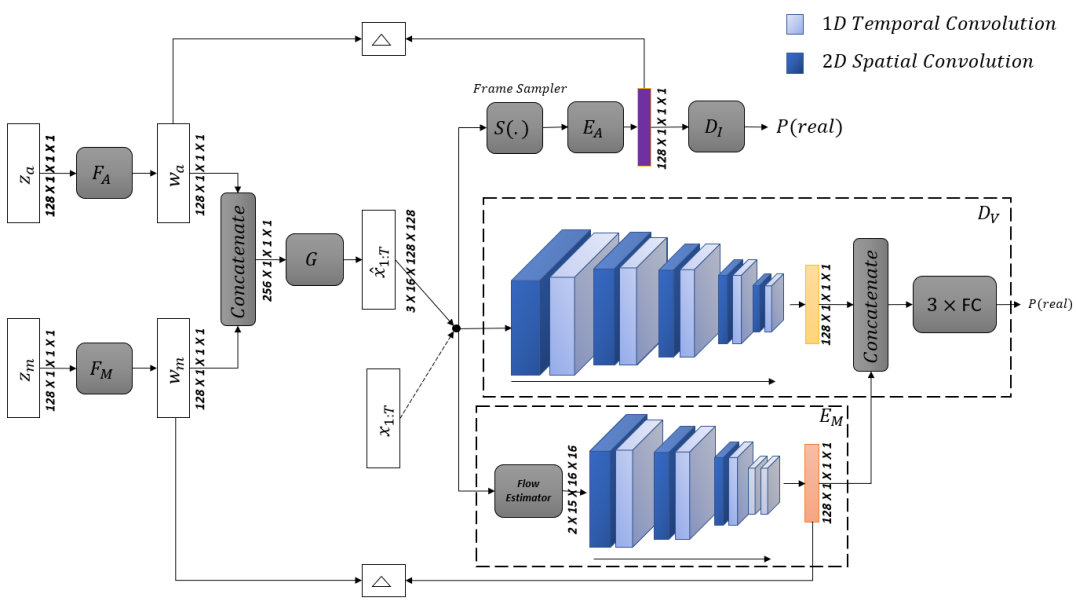
Figure 1: AVLAE architecture (best viewed in color). $F_{A}$ and $F_{M}$ project input appearance and motion latent vectors onto intermediate latent space. The video generator $G$ outputs generated video of resolution $128\times 128\times 16$ from the concatenated intermediate latent vector. The motion encoder $E_{M}$ and appearance encoder $E_{A}$ encodes motion, appearance characteristics to latent space respectively. The output dimensions are of the form $channels\times depth\times Height\times Width$. $\Delta$ denotes L1 reconstruction loss.

3 GAN Preliminaries

A GAN contains two networks, a generator $G$ and a discriminator $D$, which are trained in adversarial fashion. The generator is trained to model the data distribution and generate realistic samples by taking noise vector $z$ sampled from fixed prior $P_{Z}$ (usually gaussian), as input. Concurrently discriminator which takes the generated samples $G(z)$ and samples from data distribution $P_{\mathcal{D}}$, is trained to distinguish between them and also provides feedback to the generator.

$$\begin{split}\min_{G}\max_{D}\mathcal{L}(G,D)=\mathbb{E}_{x\sim P_{\mathcal{D}}(x)}[\log D(x)]+\\ \mathbb{E}_{z\sim P_{Z}(z)}[\log(1-D(G(z)))]\end{split}$$ (1)

The training of a GAN includes optimizing eq.1 which resembles a zero-sum game between generator and discriminator until they converge to a stable nash equilibrium. With enough capacity of $G$ and $D$, it was shown that the generator distribution $P_{G}$ converges to the real data distribution $P_{\mathcal{D}}$ allowing us to sample novel and realistic data samples [16].

4 Approach

In this section, we introduce the architecture of the proposed model. We decompose the generator of a typical GAN into three networks $F_{A}$, $F_{M}$ and $G$. $F_{A}$ and $F_{M}$ are the non-linear transformation functions for appearance and motion latent vectors respectively. They map the respective latent vectors sampled from input latent subspace to the intermediate latent subspace. $G$ is a spatio-temporal generator which outputs the generated video of fixed number of frames. On the other side, we retain the video discriminator $D_{V}$ [52, 58] and decompose the image discriminator into the appearance encoder $E_{A}$ and the image latent discriminator $D_{I}$. The image discriminator requires generator to output videos with coherent spatial structures in each frame while video discriminator requires the generated videos to be spatio-temporally consistent. We also introduce the motion encoder $E_{M}$ network which explicitly encodes the dynamics of the input video to a bottleneck representation. see Fig.1

4.1 Video Generator

We implement $F_{A}$ and $F_{M}$ as stacked fully connected layers with leaky relu activations between them and $G$ as a simple spatio-temporal upsampling generator with factorized (1+2)D transpose convolutions [51]. $F_{A}$ projects the input vector $z_{A}$ sampled from normal distribution onto the intermediate appearance subspace $W_{A}$. Similarly $F_{M}$ projects another independent vector $z_{M}$ sampled from identical distribution onto the intermediate motion subspace $W_{M}$. We aim $W_{A}$ to learn motion independent appearance features of the video and $W_{M}$ to learn disentangled motion characteristics. Appearance and motion projections are then concatenated to form samples in intermediate video latent space $W_{V}$. i.e. $W_{V}$ = $W_{A}\times W_{M}$. Network $G$ takes the concatenated vector and translates to a video of fixed frame length, $T$. So the generated video distribution would be

$$\begin{split}P_{G}(x)=\int_{w_{A}}\int_{w_{M}}P_{G}(x/w_{A},w_{M})\,P_{F_{A}}(w_{A})\\ P_{F_{M}}(w_{M})\,dw_{A}\,dw_{M}\end{split}$$ (2)

4.2 Image and Motion Encoders

Given an input video, we want our motion encoder $E_{M}$ to explicitly encode the dynamics of the video in a representational space. Optical Flow is the motion of image pixel intensities between the frames in a scene which can be attributed to motion of objects in the scene. It carries low-level motion information which can further be utilized in high-level vision tasks like video recognition [47] and even in video generation [38]. Optical flow estimation with deep neural networks has achieved great progress over the traditional methods [14, 22, 49]. Our motion encoder first estimates the optical flow sequence of length $T-1$ for the input video of $T$ frames with a pre-trained flow prediction network, which is further processed by factorized spatio-temporal convolution layers to output the encoded motion vector. Thus obtained encoded motion vector is concatenated before the fully connected layers of video discriminator as shown in Fig.1 to ensure temporal coherence in generated videos. We used the state-of-the-art end-to-end differentiable flow estimator RAFT [49] pretrained on sintel dataset [6] for obtaining optical flow at $1/8^{th}$ of the spatial resolution of the input video. The distribution at the output of motion encoder for input generated video is

$$\begin{split}P_{E_{M}}(w^{\prime}_{M})=\int_{x}P_{E_{M}}(w^{\prime}_{M}/x)\,P_{G}(x)\,dx\end{split}$$ (3)

We also sample randomly a single frame from the input video and feed it to the appearance encoder $E_{A}$ to get appearance latent vector. The encoded image is further passed to $D_{I}$ to get real/fake probabilities. If the distribution of all generated frames is $P_{G}(x_{t})$,

$$\begin{split}P_{E_{A}}(w^{\prime}_{A})=\int_{x_{t}}P_{E_{A}}(w^{\prime}_{A}/x_{t})\,P_{G}(x_{t})\,dx_{t}\end{split}$$ (4)

would be the output distribution of $E_{A}$. We observe that by training with adversarial objective, the generator distribution converges towards the real data distribution. i.e. $P_{G}(x)\approx P_{\mathcal{D}}(x)$ and $P_{G}(x_{t})\approx P_{\mathcal{D}}(x_{t})$, where $P_{\mathcal{D}}(x)$ and $P_{\mathcal{D}}(x_{t})$ are real video and real frame distribution respectively. So by replacing $P_{\mathcal{D}}(x)$, $P_{\mathcal{D}}(x_{t})$ for $P_{G}(x)$, $P_{G}(x_{t})$ in eq. 3,4 respectively, the encoder distributions converge to same for real video/frame and generated video/frame inputs.

Now the intermediate latent distributions $P_{F_{A}}(w_{A})$, $P_{F_{M}}(w_{M})$, $P_{E_{A}}(w^{\prime}_{A})$ and $P_{E_{M}}(w^{\prime}_{M})$ are not enforced to follow any predefined prior and are free to learn from the data. Additionally we put the constraint that the latent space pairs $(P_{F_{A}}(w_{A}),P_{F_{M}}(w_{M}))$ and $(P_{E_{A}}(w^{\prime}_{A}),P_{E_{M}}(w^{\prime}_{M}))$ should be same. That is,

$$\begin{split}P_{F_{A}}(w_{A})=P_{E_{A}}(w^{\prime}_{A})\\ P_{F_{M}}(w_{M})=P_{E_{M}}(w^{\prime}_{M})\end{split}$$ (5)

With this constraint, the networks $G$ - $(E_{A},E_{M})$ become generator - two stream encoder type autoencoder which autoencodes the joint video latent space $W_{V}$. We implement this constraint by a reconstruction loss between $(w_{A},w_{M})$ and $(w^{\prime}_{A},w^{\prime}_{M})$ which is minimized by updating $G$,$E_{M}^{*}$ and $E_{A}$ where $E_{M}^{*}$ represents motion encoder excluding the flow estimator network.

Algorithm 1 AVLAE Training

1:$\theta_{E_{M}^{*}}\leftarrow\theta_{E_{M}}-params(FlowEstimator)$

2:$\theta_{F_{A}},\theta_{F_{M}},\theta_{G},\theta_{E_{A}},\theta_{E_{M}^{*}},\theta_{D_{I}},\theta_{D_{V}}\leftarrow$ Initialize network parameters

3:while not converged do

4:    Step I. Update $E_{A}$, $E_{M}^{*}$, $D_{I}$ and $D_{V}$

5:    $x\leftarrow$ Random mini-batch from dataset $\mathcal{D}$

6:    $z_{A}\leftarrow$ Samples from prior $P_{Z_{A}}=\mathcal{N}(0,I)$

7:    $z_{M}\leftarrow$ Samples from prior $P_{Z_{M}}=\mathcal{N}(0,I)$

8:    $\hat{x}\leftarrow G(F_{A}(z_{A}),F_{M}(z_{M}))$

9:    $x_{t}\sim\{x_{1:T}\}$ and $\hat{x}_{t}\sim\{\hat{x}_{1:T}\}$

10:    $L^{E_{M}^{*},D_{V}}_{adv}\leftarrow\log(D_{V}(x,E_{M}(x)))+\log(1-D_{V}(\hat{x},E_{M}(\hat{x})))$

11:    $L^{E_{A},D_{I}}_{adv}\leftarrow\log(D_{I}(E_{A}(x_{t})))+\log(1-D_{I}(E_{A}(\hat{x_{t}})))$

12:    $grad\leftarrow\nabla_{\theta_{E_{M}^{*}},\theta_{D_{V}}}L^{E_{M}^{*},D_{V}}_{adv}$

13:    $\theta_{E_{M}^{*}},\theta_{D_{V}}\leftarrow\textsc{Adam}(grad,\theta_{E_{M}^{*}},\theta_{D_{V}},\alpha,\beta_{1},\beta_{2})$

14:    $grad\leftarrow\nabla_{\theta_{E_{A}},\theta_{D_{I}}}L^{E_{A},D_{I}}_{adv}$

15:    $\theta_{E_{A}},\theta_{D_{I}}\leftarrow\textsc{Adam}(grad,\theta_{E_{A}},\theta_{D_{I}},\alpha,\beta_{1},\beta_{2})$

16:    Step II. Update $F_{A}$, $F_{M}$ and $G$

17:    $z_{A}\leftarrow$ Samples from prior $P_{Z_{A}}=\mathcal{N}(0,I)$

18:    $z_{M}\leftarrow$ Samples from prior $P_{Z_{M}}=\mathcal{N}(0,I)$

19:    $\hat{x}\leftarrow G(F_{A}(z_{A}),F_{M}(z_{M}))$

20:    $\hat{x}_{t}\sim\{\hat{x}_{1:T}\}$

21:    $L^{F_{A},F_{M},G}_{adv}\leftarrow\log(1-D_{I}(E_{A}(\hat{x}_{t})))+\log(1-D_{V}(E_{M}(\hat{x})))$

22:    $grad\leftarrow\nabla_{\theta_{F_{A}},\theta_{F_{M}},\theta_{G}}L^{F_{A},F_{M},G}_{adv}$

23:    $\theta_{F_{A}},\theta_{F_{M}},\theta_{G}\leftarrow\textsc{Adam}(grad,\theta_{F_{A}},\theta_{F_{A}},\theta_{G},\alpha,\beta_{1},\beta_{2})$

24:    Step III. Update $E_{A}$, $E_{M}^{*}$ and $G$

25:    $z_{A}\leftarrow$ Samples from prior $P_{Z_{A}}=\mathcal{N}(0,I)$

26:    $z_{M}\leftarrow$ Samples from prior $P_{Z_{M}}=\mathcal{N}(0,I)$

27:    $L^{E_{A},E_{M}^{*},G}_{rec}\leftarrow\|F_{M}(z_{M})-E_{M}(G(F_{A}(z_{A}),F_{M}(z_{M})))\|_{2}^{2}+\|F_{A}(z_{A})-E_{A}(G(F_{A}(z_{A}),F_{M}(z_{M}))_{t\sim\{1:T\}})\|_{2}^{2}$

28:    $grad\leftarrow\nabla_{\theta_{E_{A}},\theta_{E_{M}^{*}},\theta_{G}}L^{E_{A},E_{M}^{*},G}_{rec}$

29:    $\theta_{E_{A}},\theta_{E_{M}^{*}},\theta_{G}\leftarrow\textsc{Adam}(grad,\theta_{E_{A}},\theta_{E_{M}^{*}},\theta_{G},\alpha,\beta_{1},\beta_{2})$

30:end while

4.3 Learning

Let $T>0$ be the number of frames to be generated and $x_{1:T}$ represents the video sample of T frames from the dataset $\mathcal{D}$. Let $z_{A}$ and $z_{M}$ are appearance and motion latent vector samples from input latent subspaces $Z_{A}$ and $Z_{M}$ respectively. Then the adversarial objective of our framework is

$$\begin{split}\min_{F_{A},F_{M},G}\,\,\max_{E_{A},E_{M}^{*},D_{I},D_{V}}\mathcal{L}_{adv}(F_{A},F_{M},G,E_{A},E_{M},D_{I},D_{V})\end{split}$$ (6)

where

$$\begin{split}\mathcal{L}_{adv}(F_{A},F_{M},G,E_{A},E_{M},D_{I},D_{V})=\\ \mathcal{L}_{I}(F_{A},F_{M},G,E_{A},D_{I})+\mathcal{L}_{V}(F_{A},F_{M},G,E_{M},D_{V})\end{split}$$ (7)

$\mathcal{L}_{I}$ and $\mathcal{L}_{V}$ are the adversarial losses from $D_{I}$ and $D_{V}$ respectively. Let $\hat{x}_{1:T}=G(F_{A}(z_{A}),F_{M}(z_{M}))$ be the generated video.

$$\begin{split}\mathcal{L}_{V}(F_{A},F_{M},G,E_{M},D_{V})=\mathbb{E}_{x}[\log D_{V}(x,E_{M}(x))]+\\ \mathbb{E}_{z_{A},z_{M}}[\log(1-D_{V}(\hat{x},E_{M}(\hat{x})))]\end{split}$$ (8)

$$\begin{split}\mathcal{L}_{I}(F_{A},F_{M},G,E_{A},D_{I})=\mathbb{E}_{x_{t}}[\log D_{I}(E_{A}(x_{t}))]+\\ \mathbb{E}_{z_{A},z_{M}}[\log(1-D_{I}(E_{A}(\hat{x}_{t\sim\{1:T\}})))]\end{split}$$ (9)

where $\mathbb{E}_{x}$, $\mathbb{E}_{z_{A},z_{M}}$, $\mathbb{E}_{x_{t}}$ are short-hands for $\mathbb{E}_{x\sim P_{\mathcal{D}}(x)}$, $\mathbb{E}_{z_{A}\sim P_{Z_{A}}(z_{A}),z_{M}\sim P_{Z_{M}}(z_{M})}$ and $\mathbb{E}_{x_{t}\sim P_{\mathcal{D}}(x_{t})}$ respectively. We also additionally optimize over the following objective to enforce the constraint eq.5.

$$\begin{split}\min_{E_{A},E_{M}^{*},G}\,\mathcal{L}_{rec}(G,E_{A},E_{M})=K_{1}\|F_{M}(z_{M})-E_{M}(\hat{x})\|_{2}^{2}+\\ K_{2}\|F_{A}(z_{A})-E_{A}(\hat{x}_{t\sim\{1:T\}})\|_{2}^{2}\end{split}$$ (10)

We update the respective networks to optimize w.r.t. eq.6,10 in alternative steps in each iteration. We summarized our training algorithm in alg.1. We note that the flow estimator is not updated in any of the steps and only passes the gradients to the generator.

5 Experiments

We compare our approach with state-of-the art GAN based video generation methods VGAN [56], TGAN [44], MoCoGAN [52] and G³AN [58] which are closest to our work, qualitatively and quantitatively. Then we conduct experiments to demonstrate the motion and content disentanglement by manipulating the latent spaces. Finally we perform ablation studies for our proposed method to show the effectiveness of each component of the architecture.

5.1 Datasets

We evaluate the proposed method on three datasets namely UvA-NEMO smiles [12], Weizmann Human Actions [4] and UCF-101 Action Recognition [48] datasets.

UvA-NEMO smiles dataset consists of 1240 spontaneous/posed smiling video sequences spanning around 400 identities. The Weizmann Human Actions dataset comprises 90 videos of 9 people performing 10 natural actions. Similar to [58], we augment the dataset by horizontally flipping the videos. The UCF-101 is a more diverse 101 category actions dataset with videos collected from YouTube. We resize each frame to $170\times 128$ resolution and center crop to $128\times 128$.

5.2 Implementation Details

We trained our model using PyTorch for generating $128\times 128$ spatial resolution videos with $T=16$ frames. We used ADAM optimizer [29] with $\beta_{1}=0.5$ and $\beta_{2}=0.999$ and a learning rate of $2e^{-4}$ for all networks. All our latent vectors $z_{A}$,$z_{M}$,$w_{A}$ and $w_{M}$ are 128 dimensional vectors. We used $K_{1}=K_{2}=1$ in eq.10 in all our experiments. The networks $F_{A}$,$F_{M}$ are independent and implemented as 5 stacked fully connected layers each while $D_{I}$ and $D_{V}$ are 3 stacked fully connected layers each. Through out our framework, we used factorized versions of 3D convolutional and 3D transpose convolutional layers.

5.3 Quantitative Analysis

We evaluate each method quantitatively with two metrics which are video extensions of widely used image generation evaluation metrics, Fréchet Inception Distance (FID) [19] on all aforementioned datasets and Inception Score (IS) [46] on UCF-101 dataset. We utilize the features of 3D CNN feature extractor [18] similar to [58], on dataset and generated video samples. The FID-Score compares for samples from dataset and generated videos, the first and second moments of the distribution of 3D CNN features. The Inception score (IS) is calculated as relative entropy between conditional and marginal distributions of classification labels for generated video samples. The FID score captures the video quality and temporal coherence. Higher inception score implies low entropy in conditional and high entropy in marginal class distributions. So IS captures both visual quality and diversity of generated videos.

We use our trained model to generate videos randomly which are to be used in FID and IS calculation. As previous methods were trained for $64\times 64$ resolution videos, we also downsample our generated videos to $64\times 64$ and report FID values on both resolutions to avoid unwarranted advantanges simply because of higher resolution. We randomly generate 5000 video samples for each trained model and utilize them in calculation of the metrics. FID and IS scores for different approaches are shown in Table.1 and Table.2 correspondingly. G³AN results are different from those reported in [58] as the authors of G³AN have improved their model in their official code.

Method	UvA	Weizmann	UCF-101
VGAN	235.01	158.04	115.06
TGAN	216.41	99.85	110.58
MoCoGAN	197.32	92.18	104.14
G3AN	64.82	76.94	87.20
AVLAE-64	60.05	68.46	84.38
AVLAE	54.20	65.71	80.59

Table 1: Video FID score comparison with state-of-the-art approaches (lower is better). All results except ours are taken from [58].

VGAN	TGAN	MoCoGAN
2.94	2.74	3.06
G3AN	AVLAE-64	AVLAE
3.88	3.93	3.97

Table 2: Video IS score comparison with state-of-the-art approaches (higher is better) on UCF-101 dataset. All results except ours are taken from [58].

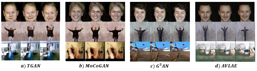
Figure 2: Visual comparison of generated samples ($1^{st}$,$10^{th}$ and $16^{th}$ frames) with TGAN, MoCoGAN and G³AN methods. Top row are generated samples from UvA-NEMO, middle row are Weizmann Action and UCF-101 samples in third row. Video frames of TGAN, G³AN and MoCoGAN are from [58].

Our approach consistently outperformed the previous methods in all datasets with respect to FID score. This manifests the superior visual quality and spatio-temporal consistency of our generated video samples. The higher inception score on UCF-101 demonstrates the diverse video samples spanning the latent space. We note that G³AN produced second best results and is closest to our approach. However, the G³AN packs an expensive generator with around 25M trainable parameters for generating $64\times 64\times 16$ videos while our generator contains nearly same number of trainable parameters for generating $128\times 128\times 16$ resolution videos.

5.4 Qualitative Analysis

We randomly sample the videos from the trained models by sampling the latent vectors and feeding them to the generator. We present generated samples by different methods on the three datasets in Fig.2.

We experiment with the motion and appearance disentanglement in the latent space. Particularly, we fix one of the input latent vectors $z_{A},z_{M}$ while varying the other and visualize the videos obtained in the process. Fig.3 shows the samples obtained while changing the motion code $z_{M}$ and keeping the appearance code $z_{A}$ same. All the three methods including ours, preserved the appearance characteristics (facial appearance) across the two samples but the motion in the samples generated by MoCoGAN is unaltered even though $z_{M}$ is changed. G³AN and AVLAE are able to alter the motion (amount of smile in this case) for different samples of $z_{M}$. This shows the efficient motion disentanglement in latent space. We note that unlike G³AN, there is no explicit structural composition of generator to achieve the same in our framework (both $z_{M}$ and $z_{A}$ are equivalent with respect to the generator’s architecture). Figure 4 further shows the alteration of appearance characteristics in generated videos by our model while changing $z_{A}$ without altering $z_{M}$.

With the input video sample from dataset distribution, the reconstructions given by the autoencoder can also be visualized by using the feature representations. For input real video $x$, we sample a single frame $x_{t\sim\{1:T\}}$ and construct the model output as $G(E_{A}(x_{t}),E_{M}(x))$. Fig. 5 shows such reconstructions for held out videos during training.

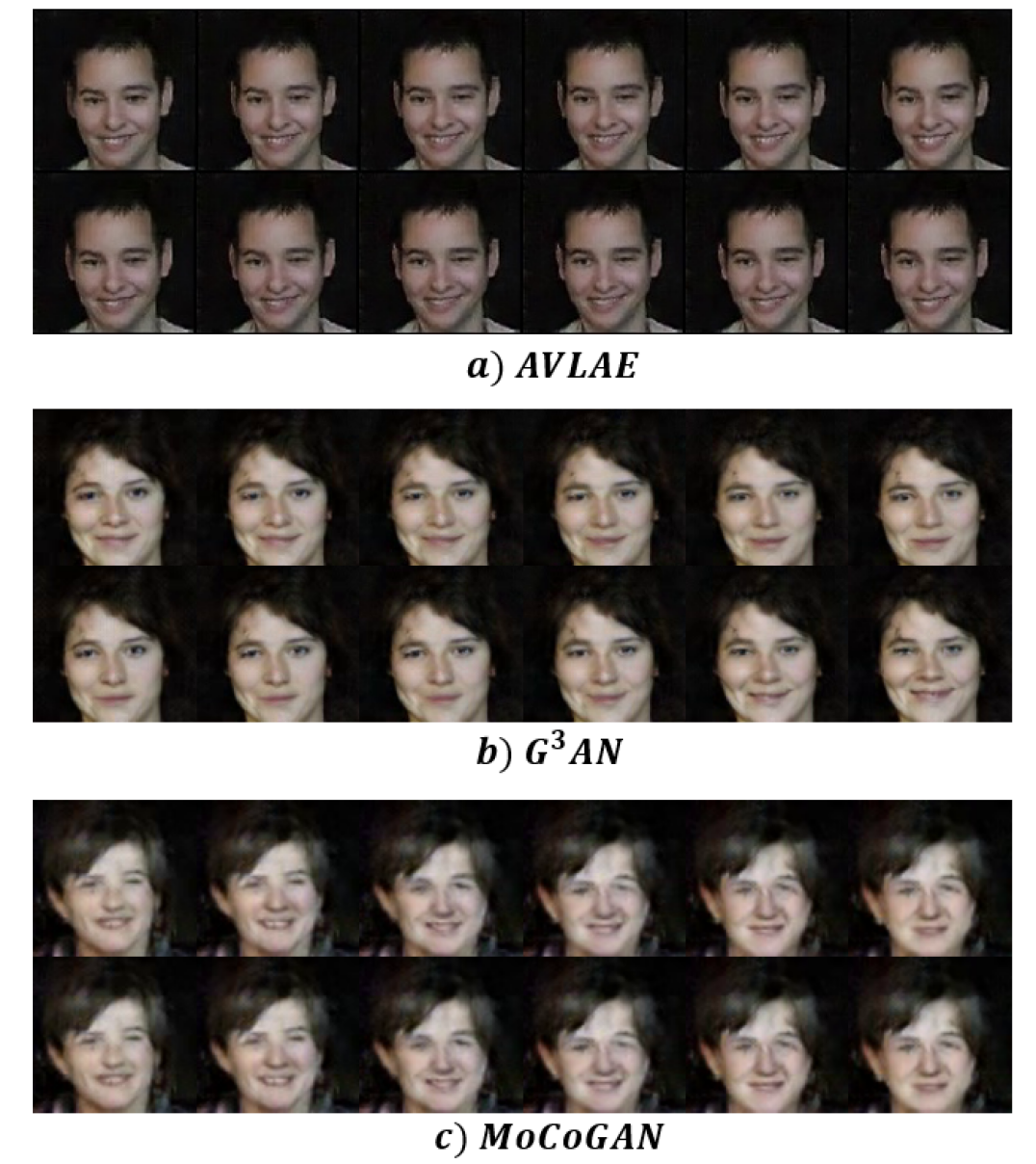
Figure 3: Video samples with same appearance code $z_{A}$ and two different samples of $z_{M}$ for each method on UvA-NEMO dataset. Best viewed when zoomed-in

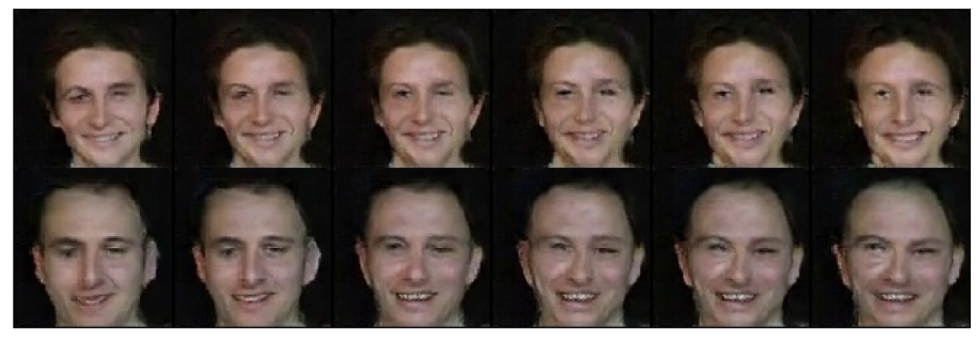
Figure 4: Video samples generated by AVLAE with same motion code $z_{M}$ and two different samples of $z_{A}$. Best viewed when zoomed-in

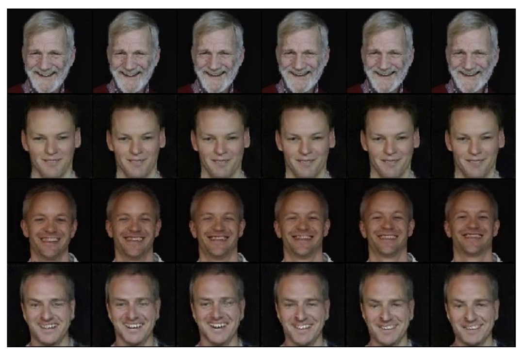
Figure 5: Reconstructions of real video samples. $1^{st}$ and $3^{rd}$ rows are the real video inputs. $2^{nd}$ and $4^{th}$ row videos are their corresponding reconstructions.

5.5 Ablation Study

Further we study the contribution of each individual component in our proposed architecture. As our main contributions are regarding latent reconstruction and motion encoder block, we retrain our model on UvA-NEMO dataset in the following four cases of modification : i) removing latent motion code $w_{M}$ reconstruction ii) removing appearance latent $w_{A}$ reconstruction iii) removing both appearance and motion latent reconstruction iv) removing both appearance and motion latent reconstructions and Motion Encoder $E_{M}$. The first three cases are equivalent to choosing hyperparameters $K_{1}=0$ , $K_{2}=0$ and $K_{1}=K_{2}=0$ respectively. Note that these three cases still include the motion encoder in their architecture. In fourth case, we remove motion encoder additionally and change the number of channels of fully connected layers in $D_{V}$ accordingly which results in normal video GAN with image and video discriminators. We evaluate these cases quantitatively in terms of FID scores on UvA-NEMO dataset in Table. 3.

Architecture	FID
AVLAE	54.20
$-w_{A}\ rec$	37.50
$-w_{M}\ rec$	59.84
$-w_{A}\ rec$, $-w_{M}\ rec$	59.28
$-w_{A}\ rec$, $-w_{M}\ rec$, $-E_{M}$	233.82

Table 3: Video FID score comparison on UvA-NEMO dataset for different modifications in architecture

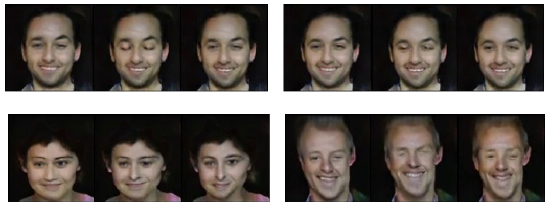
Figure 6: Ablation Study: First row shows two videos with different $z_{A}$ and same $z_{M}$ when $w_{A}$ reconstruction is removed. Second row shows two videos with same $z_{A}$ and different $z_{M}$ when $w_{M}$ reconstruction is removed.

We first observe that the motion encoder has the most effect on generating high fidelity videos with temporal consistency, as removing the motion encoder resulted in the highest rise in FID score. Further, the removal of appearance reconstruction gave best FID score overall. This is in-line with the findings of [40] that the intermediate latent space learning more discriminative features from image discriminator might not be ’rich’ enough. However the removal of appearance reconstruction resulted in the loss of control over the latent space as in, the appearance characteristics remain unaltered even when the $z_{A}$ is altered as shown in Fig. 6. Similarly we observe the appearance alteration while altering the motion vector $z_{M}$ when $w_{M}$ reconstruction is removed. This might be because of the feedback from video discriminator to the motion encoder forcing the latent subspace $W_{M}$ to learn both motion and appearance features when either of the latent spaces are left unconstrained. However removing the latent motion reconstruction also resulted in videos with unnatural motion between the frames. The intact AVLAE architecture generates high quality videos while also decomposing the motion and appearance.

6 Conclusion

In this paper, we have presented an adversarial autoencoder framework for video generation. Our work is the first autoencoder based video generative model that is able to learn video distribution efficiently and perform better than existing GAN based video generation methods. We considered a rudimentary structure for the generator and proposed to autoencode the decomposed latent vectors. The experiments demonstrated the ability of our framework to generate high fidelity videos with spatio-temporal consistency as well as to learn less entangled representations of the videos in the latent space resulting in decomposition of motion and appearance. Further ablation experiments prove that the intact AVLAE model gives more control over the latent space while preserving the video quality.

References

- [1] D. Acharya, Z. Huang, D. Paudel, and L. Gool. Towards high resolution video generation with progressive growing of sliced wasserstein gans. ArXiv, abs/1810.02419, 2018.
- [2] Martin Arjovsky, Soumith Chintala, and Léon Bottou. Wasserstein generative adversarial networks. In Doina Precup and Yee Whye Teh, editors, Proceedings of the 34th International Conference on Machine Learning, volume 70 of Proceedings of Machine Learning Research, pages 214–223, International Convention Centre, Sydney, Australia, 06–11 Aug 2017. PMLR.
- [3] Mohammad Babaeizadeh, Chelsea Finn, Dumitru Erhan, Roy H. Campbell, and Sergey Levine. Stochastic variational video prediction. In International Conference on Learning Representations, 2018.
- [4] Moshe Blank, Lena Gorelick, Eli Shechtman, Michal Irani, and Ronen Basri. Actions as space-time shapes. In The Tenth IEEE International Conference on Computer Vision (ICCV’05), pages 1395–1402, 2005.
- [5] Andrew Brock, Jeff Donahue, and Karen Simonyan. Large scale GAN training for high fidelity natural image synthesis. In International Conference on Learning Representations, 2019.
- [6] D. J. Butler, J. Wulff, G. B. Stanley, and M. J. Black. A naturalistic open source movie for optical flow evaluation. In A. Fitzgibbon et al. (Eds.), editor, European Conf. on Computer Vision (ECCV), Part IV, LNCS 7577, pages 611–625. Springer-Verlag, Oct. 2012.
- [7] Yunjey Choi, Minje Choi, Munyoung Kim, Jung-Woo Ha, Sunghun Kim, and Jaegul Choo. Stargan: Unified generative adversarial networks for multi-domain image-to-image translation. In Proceedings of the IEEE Conference on Computer Vision and Pattern Recognition (CVPR), June 2018.
- [8] Aidan Clark, Jeff Donahue, and Karen Simonyan. Adversarial video generation on complex datasets, 2019.
- [9] Emily Denton and Rob Fergus. Stochastic video generation with a learned prior. In Jennifer Dy and Andreas Krause, editors, Proceedings of the 35th International Conference on Machine Learning, volume 80 of Proceedings of Machine Learning Research, pages 1174–1183, Stockholmsmässan, Stockholm Sweden, 10–15 Jul 2018. PMLR.
- [10] Emily L Denton and vighnesh Birodkar. Unsupervised learning of disentangled representations from video. In I. Guyon, U. V. Luxburg, S. Bengio, H. Wallach, R. Fergus, S. Vishwanathan, and R. Garnett, editors, Advances in Neural Information Processing Systems, volume 30. Curran Associates, Inc., 2017.
- [11] Emily L Denton, Soumith Chintala, arthur szlam, and Rob Fergus. Deep generative image models using a laplacian pyramid of adversarial networks. In C. Cortes, N. Lawrence, D. Lee, M. Sugiyama, and R. Garnett, editors, Advances in Neural Information Processing Systems, volume 28. Curran Associates, Inc., 2015.
- [12] Hamdi Dibeklioğlu, Albert Ali Salah, and Theo Gevers. Are you really smiling at me? spontaneous versus posed enjoyment smiles. In Andrew Fitzgibbon, Svetlana Lazebnik, Pietro Perona, Yoichi Sato, and Cordelia Schmid, editors, Computer Vision – ECCV 2012, pages 525–538, Berlin, Heidelberg, 2012. Springer Berlin Heidelberg.
- [13] J. Donahue, Philipp Krähenbühl, and Trevor Darrell. Adversarial feature learning. ArXiv, abs/1605.09782, 2017.
- [14] Alexey Dosovitskiy, Philipp Fischer, Eddy Ilg, Philip Hausser, Caner Hazirbas, Vladimir Golkov, Patrick van der Smagt, Daniel Cremers, and Thomas Brox. Flownet: Learning optical flow with convolutional networks. In Proceedings of the IEEE International Conference on Computer Vision (ICCV), December 2015.
- [15] Vincent Dumoulin, Ishmael Belghazi, Ben Poole, Alex Lamb, Martín Arjovsky, Olivier Mastropietro, and Aaron C. Courville. Adversarially learned inference. ArXiv, abs/1606.00704, 2017.
- [16] Ian Goodfellow, Jean Pouget-Abadie, Mehdi Mirza, Bing Xu, David Warde-Farley, Sherjil Ozair, Aaron Courville, and Yoshua Bengio. Generative adversarial nets. In Z. Ghahramani, M. Welling, C. Cortes, N. Lawrence, and K. Q. Weinberger, editors, Advances in Neural Information Processing Systems, volume 27. Curran Associates, Inc., 2014.
- [17] Ishaan Gulrajani, Faruk Ahmed, Martin Arjovsky, Vincent Dumoulin, and Aaron C Courville. Improved training of wasserstein gans. In I. Guyon, U. V. Luxburg, S. Bengio, H. Wallach, R. Fergus, S. Vishwanathan, and R. Garnett, editors, Advances in Neural Information Processing Systems, volume 30. Curran Associates, Inc., 2017.
- [18] Kensho Hara, Hirokatsu Kataoka, and Yutaka Satoh. Can spatiotemporal 3d cnns retrace the history of 2d cnns and imagenet? In Proceedings of the IEEE Conference on Computer Vision and Pattern Recognition (CVPR), June 2018.
- [19] Martin Heusel, Hubert Ramsauer, Thomas Unterthiner, Bernhard Nessler, and Sepp Hochreiter. Gans trained by a two time-scale update rule converge to a local nash equilibrium. In I. Guyon, U. V. Luxburg, S. Bengio, H. Wallach, R. Fergus, S. Vishwanathan, and R. Garnett, editors, Advances in Neural Information Processing Systems, volume 30. Curran Associates, Inc., 2017.
- [20] Jun-Ting Hsieh, Bingbin Liu, De-An Huang, Li F Fei-Fei, and Juan Carlos Niebles. Learning to decompose and disentangle representations for video prediction. In S. Bengio, H. Wallach, H. Larochelle, K. Grauman, N. Cesa-Bianchi, and R. Garnett, editors, Advances in Neural Information Processing Systems, volume 31. Curran Associates, Inc., 2018.
- [21] Huaibo Huang, zhihang li, Ran He, Zhenan Sun, and Tieniu Tan. Introvae: Introspective variational autoencoders for photographic image synthesis. In S. Bengio, H. Wallach, H. Larochelle, K. Grauman, N. Cesa-Bianchi, and R. Garnett, editors, Advances in Neural Information Processing Systems, volume 31. Curran Associates, Inc., 2018.
- [22] Eddy Ilg, Nikolaus Mayer, Tonmoy Saikia, Margret Keuper, Alexey Dosovitskiy, and Thomas Brox. Flownet 2.0: Evolution of optical flow estimation with deep networks. In Proceedings of the IEEE Conference on Computer Vision and Pattern Recognition (CVPR), July 2017.
- [23] Phillip Isola, Jun-Yan Zhu, Tinghui Zhou, and Alexei A. Efros. Image-to-image translation with conditional adversarial networks. In Proceedings of the IEEE Conference on Computer Vision and Pattern Recognition (CVPR), July 2017.
- [24] Beibei Jin, Yu Hu, Qiankun Tang, Jingyu Niu, Zhiping Shi, Yinhe Han, and Xiaowei Li. Exploring spatial-temporal multi-frequency analysis for high-fidelity and temporal-consistency video prediction. In IEEE/CVF Conference on Computer Vision and Pattern Recognition (CVPR), June 2020.
- [25] Emmanuel Kahembwe and Subramanian Ramamoorthy. Lower dimensional kernels for video discriminators. Neural Networks, 132:506–520, 2020.
- [26] Tero Karras, Timo Aila, S. Laine, and J. Lehtinen. Progressive growing of gans for improved quality, stability, and variation. ArXiv, abs/1710.10196, 2018.
- [27] Tero Karras, Samuli Laine, and Timo Aila. A style-based generator architecture for generative adversarial networks. In Proceedings of the IEEE/CVF Conference on Computer Vision and Pattern Recognition (CVPR), June 2019.
- [28] Tero Karras, Samuli Laine, Miika Aittala, Janne Hellsten, Jaakko Lehtinen, and Timo Aila. Analyzing and improving the image quality of stylegan. In Proceedings of the IEEE/CVF Conference on Computer Vision and Pattern Recognition (CVPR), June 2020.
- [29] Diederik P. Kingma and Jimmy Ba. Adam: A method for stochastic optimization, 2017.
- [30] Diederik P. Kingma and Max Welling. Auto-encoding variational bayes. In Yoshua Bengio and Yann LeCun, editors, 2nd International Conference on Learning Representations, ICLR 2014, Banff, AB, Canada, April 14-16, 2014, Conference Track Proceedings, 2014.
- [31] Anders Boesen Lindbo Larsen, Søren Kaae Sønderby, Hugo Larochelle, and Ole Winther. Autoencoding beyond pixels using a learned similarity metric. In Maria Florina Balcan and Kilian Q. Weinberger, editors, Proceedings of The 33rd International Conference on Machine Learning, volume 48 of Proceedings of Machine Learning Research, pages 1558–1566, New York, New York, USA, 20–22 Jun 2016. PMLR.
- [32] Christian Ledig, Lucas Theis, Ferenc Huszar, Jose Caballero, Andrew Cunningham, Alejandro Acosta, Andrew Aitken, Alykhan Tejani, Johannes Totz, Zehan Wang, and Wenzhe Shi. Photo-realistic single image super-resolution using a generative adversarial network. In Proceedings of the IEEE Conference on Computer Vision and Pattern Recognition (CVPR), July 2017.
- [33] Alex X. Lee, Richard Zhang, Frederik Ebert, Pieter Abbeel, Chelsea Finn, and Sergey Levine. Stochastic adversarial video prediction, 2018.
- [34] Alireza Makhzani, Jonathon Shlens, Navdeep Jaitly, and Ian J. Goodfellow. Adversarial autoencoders. ArXiv, abs/1511.05644, 2015.
- [35] Tanya Marwah, Gaurav Mittal, and Vineeth N. Balasubramanian. Attentive semantic video generation using captions. In Proceedings of the IEEE International Conference on Computer Vision (ICCV), Oct 2017.
- [36] Michaël Mathieu, C. Couprie, and Y. LeCun. Deep multi-scale video prediction beyond mean square error. CoRR, abs/1511.05440, 2016.
- [37] Takeru Miyato, T. Kataoka, Masanori Koyama, and Y. Yoshida. Spectral normalization for generative adversarial networks. ArXiv, abs/1802.05957, 2018.
- [38] Katsunori Ohnishi, Shohei Yamamoto, Yoshitaka Ushiku, and Tatsuya Harada. Hierarchical video generation from orthogonal information: Optical flow and texture. Proceedings of the AAAI Conference on Artificial Intelligence, 32(1), Apr. 2018.
- [39] Junting Pan, Chengyu Wang, Xu Jia, Jing Shao, Lu Sheng, Junjie Yan, and Xiaogang Wang. Video generation from single semantic label map. In Proceedings of the IEEE/CVF Conference on Computer Vision and Pattern Recognition (CVPR), June 2019.
- [40] Stanislav Pidhorskyi, Donald A. Adjeroh, and Gianfranco Doretto. Adversarial latent autoencoders. In IEEE/CVF Conference on Computer Vision and Pattern Recognition (CVPR), June 2020.
- [41] A. Radford, Luke Metz, and Soumith Chintala. Unsupervised representation learning with deep convolutional generative adversarial networks. CoRR, abs/1511.06434, 2016.
- [42] Kevin Roth, Aurelien Lucchi, Sebastian Nowozin, and Thomas Hofmann. Stabilizing training of generative adversarial networks through regularization. In I. Guyon, U. V. Luxburg, S. Bengio, H. Wallach, R. Fergus, S. Vishwanathan, and R. Garnett, editors, Advances in Neural Information Processing Systems, volume 30. Curran Associates, Inc., 2017.
- [43] D. E. Rumelhart and J. L. McClelland. Learning Internal Representations by Error Propagation, pages 318–362. 1987.
- [44] Masaki Saito, Eiichi Matsumoto, and Shunta Saito. Temporal generative adversarial nets with singular value clipping. In Proceedings of the IEEE International Conference on Computer Vision (ICCV), Oct 2017.
- [45] Masaki Saito, Shunta Saito, Masanori Koyama, and S. Kobayashi. Train sparsely, generate densely: Memory-efficient unsupervised training of high-resolution temporal gan. International Journal of Computer Vision, pages 1–21, 2020.
- [46] Tim Salimans, Ian Goodfellow, Wojciech Zaremba, Vicki Cheung, Alec Radford, Xi Chen, and Xi Chen. Improved techniques for training gans. In D. Lee, M. Sugiyama, U. Luxburg, I. Guyon, and R. Garnett, editors, Advances in Neural Information Processing Systems, volume 29. Curran Associates, Inc., 2016.
- [47] Karen Simonyan and Andrew Zisserman. Two-stream convolutional networks for action recognition in videos. In Z. Ghahramani, M. Welling, C. Cortes, N. Lawrence, and K. Q. Weinberger, editors, Advances in Neural Information Processing Systems, volume 27. Curran Associates, Inc., 2014.
- [48] K. Soomro, A. Zamir, and M. Shah. Ucf101: A dataset of 101 human actions classes from videos in the wild. ArXiv, abs/1212.0402, 2012.
- [49] Zachary Teed and Jia Deng. Raft: Recurrent all-pairs field transforms for optical flow. In Andrea Vedaldi, Horst Bischof, Thomas Brox, and Jan-Michael Frahm, editors, Computer Vision – ECCV 2020, pages 402–419, Cham, 2020. Springer International Publishing.
- [50] Yu Tian, Jian Ren, Menglei Chai, Kyle Olszewski, Xi Peng, Dimitris N. Metaxas, and Sergey Tulyakov. A good image generator is what you need for high-resolution video synthesis. In International Conference on Learning Representations, 2021.
- [51] Du Tran, Heng Wang, Lorenzo Torresani, Jamie Ray, Yann LeCun, and Manohar Paluri. A closer look at spatiotemporal convolutions for action recognition. In Proceedings of the IEEE Conference on Computer Vision and Pattern Recognition (CVPR), June 2018.
- [52] Sergey Tulyakov, Ming-Yu Liu, Xiaodong Yang, and Jan Kautz. Mocogan: Decomposing motion and content for video generation. In Proceedings of the IEEE Conference on Computer Vision and Pattern Recognition (CVPR), June 2018.
- [53] Dmitry Ulyanov, Andrea Vedaldi, and Victor Lempitsky. It takes (only) two: Adversarial generator-encoder networks. In Proceedings of the AAAI Conference on Artificial Intelligence, volume 32, 2018.
- [54] R. Villegas, Jimei Yang, Seunghoon Hong, Xunyu Lin, and H. Lee. Decomposing motion and content for natural video sequence prediction. ArXiv, abs/1706.08033, 2017.
- [55] Ruben Villegas, Jimei Yang, Yuliang Zou, Sungryull Sohn, Xunyu Lin, and Honglak Lee. Learning to generate long-term future via hierarchical prediction. In Doina Precup and Yee Whye Teh, editors, Proceedings of the 34th International Conference on Machine Learning, volume 70 of Proceedings of Machine Learning Research, pages 3560–3569, International Convention Centre, Sydney, Australia, 06–11 Aug 2017. PMLR.
- [56] Carl Vondrick, Hamed Pirsiavash, and Antonio Torralba. Generating videos with scene dynamics. In D. Lee, M. Sugiyama, U. Luxburg, I. Guyon, and R. Garnett, editors, Advances in Neural Information Processing Systems, volume 29. Curran Associates, Inc., 2016.
- [57] Tsun-Hsuan Wang, Yen-Chi Cheng, Chieh Hubert Lin, Hwann-Tzong Chen, and Min Sun. Point-to-point video generation. In Proceedings of the IEEE/CVF International Conference on Computer Vision (ICCV), October 2019.
- [58] Yaohui Wang, Piotr Bilinski, Francois Bremond, and Antitza Dantcheva. G3an: Disentangling appearance and motion for video generation. In IEEE/CVF Conference on Computer Vision and Pattern Recognition (CVPR), June 2020.
- [59] Wei Yu, Yichao Lu, Steve Easterbrook, and Sanja Fidler. Efficient and information-preserving future frame prediction and beyond. In International Conference on Learning Representations, 2020.
- [60] Han Zhang, Ian Goodfellow, Dimitris Metaxas, and Augustus Odena. Self-attention generative adversarial networks. In Kamalika Chaudhuri and Ruslan Salakhutdinov, editors, Proceedings of the 36th International Conference on Machine Learning, volume 97 of Proceedings of Machine Learning Research, pages 7354–7363. PMLR, 09–15 Jun 2019.
- [61] Jun-Yan Zhu, Taesung Park, Phillip Isola, and Alexei A. Efros. Unpaired image-to-image translation using cycle-consistent adversarial networks. In Proceedings of the IEEE International Conference on Computer Vision (ICCV), Oct 2017.