A Giant Arc on the Sky

Abstract

We present the serendipitous discovery of a ‘Giant Arc on the Sky’ at $z\sim 0.8$. The Giant Arc (GA) spans $\sim 1$ Gpc (proper size, present epoch), and appears to be almost symmetrical on the sky. It was discovered via intervening Mg II absorbers in the spectra of background quasars, using the catalogues of Zhu & Ménard. The use of Mg II absorbers represents a new approach to the investigation of large-scale structures (LSSs) at redshifts $0.45\la z\la 2.25$. We present the observational properties of the GA, and we assess it statistically using methods based on: (i) single-linkage hierarchical clustering ($\sim 4.5\sigma$); (ii) the Cuzick-Edwards test ($\sim 3.0\sigma$); and (iii) power spectrum analysis ($\sim 4.8\sigma$). Each of these methods has distinctive attributes and powers, and we advise considering the evidence from the ensemble. We discuss our approaches to mitigating any post-hoc aspects of analysing significance after discovery. The overdensity of the GA is $\delta\rho/\rho\sim 1.3\pm 0.3$. The GA is the newest and one of the largest of a steadily accumulating set of very large LSSs that may (cautiously) challenge the Cosmological Principle, upon which the ‘standard model’ of cosmology is founded. Conceivably, the GA is the precursor of a structure like the Sloan Great Wall (but the GA is about twice the size), seen when the Universe was about half its present age.

1 Introduction

We are using intervening Mg II absorbers to investigate cosmological structure at redshifts $0.45\la z\la 2.25$. Previous work at such redshifts has generally depended on either: (i) quasars, for which there are accurate spectroscopic redshifts, or (ii) galaxies (and clusters), for which there are typically only somewhat less accurate photometric redshifts. With Mg II absorbers, however, we can obtain accurate spectroscopic redshifts for faint galaxies, subject, of course, to the limitations that the detected galaxies will be relatively sparse and that they can be only at the sky coordinates of the background quasars that are used as probes. These limitations need not, however, be a restriction on investigating large-scale structure (LSS).

In this way, we have serendipitously discovered a ‘Giant Arc on the Sky’ at $z\sim 0.8$. The Giant Arc (GA) spans $\sim 1$ Gpc (proper size, present epoch), and appears to be intriguingly symmetrical on the sky. It is one of the largest of a steadily accumulating set of very large LSSs that may (cautiously) challenge the Cosmological Principle (CP), upon which the ‘standard model’ of cosmology is founded. (Note that the word ‘challenge’ is not synonymous with ‘contradict’, but it does imply something to be investigated further.)

1.1 The largest large-scale structures

(Yadav et al.2010) gave $\sim 370$ Mpc as an ideal or upper limit to the scale of homogeneity in the concordance cosmology, beyond which departures from homogeneity should not be evident. As (Yadav et al.2010) state, above this scale it should not be possible to distinguish a given point distribution from a homogeneous distribution. We can therefore take $\sim 370$ Mpc as an indication of the size (and, incidentally, separation also) beyond which LSSs becomes cosmologically interesting. We list in Table LABEL:tab:lss_list some of the very large LSSs that have been reported in the literature, noting mainly those of (present-epoch) size $\ga 370$ Mpc. Many of the sizes quoted in this table will be somewhat uncertain, usually because of uncertainty in the boundaries, but sometimes because of uncertainty in what is being quoted in the papers (e.g. cosmological model and parameters, cosmological epoch). Also, in the lower part of Table LABEL:tab:lss_list, we list some results that, while not strictly being instances of LSS, are certainly of interest for considering the validity of the CP.

1.2 The Mg II approach

The presence of metal-rich intervening absorption lines in the spectra of quasars reveals foreground gas associated with galaxies. Specifically, the prominent and distinctive Mg II doublet feature, which can be seen over a broad range of redshifts, $0.45\la z\la 2.25$, is strongly associated with the low-ionised gas around galaxy haloes, and is therefore an easily identifiable tracer of galaxies. In particular, Mg II is known to trace the H I regions indicative of star-formation regions. Mg II absorbers can be expected to be useful tracers of large-scale structure as they trace metal-enriched gas associated with galaxies and clusters.

It is generally believed that the strength of the absorption doublet (rest equivalent widths $W_{r,2796},W_{r,2803}$) arising in the haloes corresponds to the properties of the galaxy and galaxy clusters, although there is still uncertainty about the relative importance of morphology, luminosity, impact parameter, galaxy inclination etc., and combinations of these, that lead to the different classes (weak, strong) of absorbers. See for example: Lanzetta & Bowen (1990); Churchill et al. (2000); Steidel et al. (2002); Churchill et al. (2005); Chen et al. (2010); Bordoloi et al. (2011).

The roughly spherical haloes hosting strong Mg II systems are considered to extend to radii $43\leq r\leq 88$ kpc (Kacprzak et al., 2008). It has been suggested by Steidel (1995) and Churchill et al. (2005) that Mg II absorption with rest-frame equivalent width $W_{r,2796}<0.3$ Å occurs predominantly in the outer regions of a halo, whereas stronger absorption with $W_{r,2796}>0.3$ Å occurs predominantly in the inner regions. Such an association of equivalent width with radius is seen also in C IV and Lyman-limit absorption systems. Of course, there is probably patchy structure so generalisations may be misleading.

(Lee et al.2021) investigate the rate of Mg II absorption in and around clusters of galaxies. They find that although the detection rate per quasar is higher inside the clusters, the rate is in fact quite low when considering the number of galaxies in the clusters — that is, the galaxy-to-absorber ratio is lower inside clusters, presumably because the environment within clusters modifies the galaxy haloes.

1.2.1 Data sources

We have constructed our Mg II absorber database from the Zhu & Ménard (Z&M) catalogues that are publicly available at the website https://www.guangtunbenzhu.com/jhu-sdss-metal-absorber-catalog. We have used their DR7 and DR12 ‘Trimmed’ catalogues (not the ‘Expanded’ versions). DR7 and DR12 indicate that the sources of the quasars that have been used as background probes are data releases 7 and 12 of the Sloan Digital Sky Survey (SDSS). The detection of the absorbers and the construction of the catalogues is described in Zhu & Ménard (2013) and the above website.

We paired the Z&M absorber catalogues on RA, Dec to the ‘cleaned’ quasar databases DR7QSO (Schneider et al., 2010) and DR12Q (Pâris et al., 2017). Thus the absorbers can all be associated subsequently with either DR7QSO or DR12Q.

We removed entries for repeat spectra (see the above website) within the Z&M DR12(Q) absorber catalogue, thus avoiding duplication of absorbers. There were no entries for repeat spectra within the Z&M DR7(QSO) absorber catalogue.

When a particular absorber (RA, Dec, $z$) appeared in both the Z&M DR7(QSO) and DR12(Q) catalogues, we removed the DR7(QSO) entry, thus giving preference to DR12(Q) parameters. The final database has 63876 Mg II absorbers.

We also produced a corresponding database of probes from the Z&M ‘Quasars searched’ catalogues, similarly restricting them to those that appear in either DR7QSO or DR12Q. This database has 123351 member quasars.

1.3 Cosmological model

The concordance model is adopted for cosmological calculations, with $\Omega_{T0}=1$, $\Omega_{M0}=0.27$, $\Omega_{\Lambda 0}=0.73$, and $H_{0}=70$ kms^-1Mpc^-1. All sizes given are proper sizes at the present epoch. (For consistency, we are using the same values for the cosmological parameters that were used by Clowes et al. (2013).)

2 The Giant Arc

The Giant Arc (GA) is a large, filamentary, crescent-shaped structure that was discovered serendipitously in Mg II catalogues (Zhu & Ménard, 2013). The GA extends $\sim 1$ Gpc (proper size, present epoch) in its longest dimension, at a redshift of $z\sim 0.8$. We now discuss: the discovery of the GA; observational properties; connectivity and statistical properties; overdensity and comparisons with other data.

2.1 Discovery of the Giant Arc

The discovery and the preliminary analysis of the GA were first discussed in Lopez (2019) and are briefly summarised here. The GA was discovered when testing the Mg II approach on six small fields containing published structures (e.g. clusters and superclusters) at $z\ga 0.7$. The Sunyaev-Zeldovich (SZ) cluster candidate PSZ2 G069.39+68.05 (Burenin et al., 2018, subsequently B18), at $z=0.763$, was one such field: it indicated a very large LSS extending on the sky, as a dense, long, thin band of Mg II absorbers, roughly symmetrically to both sides of the cluster. In Lopez (2019) the central redshift and the redshift interval of the GA were estimated by stepping through thin redshift slices and visually inspecting the density and connectivity of the Mg II absorbers. We have since refined a little the estimates of the central redshift and the redshift interval — see Section 2.3.1 for the details. In Fig. 1 the GA can be seen stretching $\sim 1$ Gpc (proper distance, present epoch) horizontally across the centre of the field. Visually, the GA appears densely concentrated and with the distinctive shape of a giant arc.

The Mg II density images, such as Fig. 1 here, and others throughout, are intended to give a useful impression of the connectivity of the absorbers. The images are constructed by smoothing the 2D distributions of the Mg II absorbers and the background probes (quasars) with a Gaussian kernel, with the same smoothing scale for both. In a process of ‘flat-fielding’ the absorber image is then divided by the normalised probe image to correct for non-uniformities in the distribution of the probes on that smoothing scale. The grey contours in the Mg II density images increase by a factor of two. We use tangent-plane coordinates, scaled, using the central redshift, to present-epoch proper coordinates in Mpc.

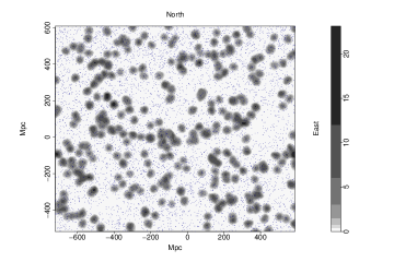
Figure 1: The tangent-plane distribution of Mg II absorbers centred in the redshift interval $z=0.802\pm 0.060$. The grey contours, increasing by a factor of two, represent the density distribution of the absorbers which have been smoothed using a Gaussian kernel of $\sigma=11$ Mpc, and flat-fielded with respect to the distribution of background probes. The dark blue dots represent the background probes (quasars). The axes are labelled in Mpc, scaled to the present epoch. East is towards the right and north is towards the top. The GA runs west-east in the centre of the figure, spanning $\sim 1$ Gpc.

2.2 Observational properties of the Giant Arc

We investigate the observational properties of the GA, in a visual manner, including: equivalent width (EW) distribution ($W_{r,2796}$); signal-to-noise ratio (S/N) of the $\lambda 2796$ Mg II line; S/N of the continuum of the spectra; the $i$ magnitude ($i$) of the probes (background quasars); and the redshift distribution ($z_{2796}$). Previously, we noted that EW distribution could be related to the galaxy properties (morphology, luminosity, impact parameter, galaxy inclination etc.), but these aspects are still not fully understood. While it may not yet be clear what the EW distribution within the GA indicates, future studies of EW in Mg II data should ultimately lead to more understanding of the origins of the GA and its environment.

The values of the EW are often classed as ‘strong’ or ‘weak’, although there seems to be no agreement on what defines ‘strong’ and ‘weak’. For example, in the literature one might find strong EW variously defined as $W_{r,2796}\geq 0.3$ Å, $W_{r,2796}\geq 0.6$ Å, and $W_{r,2796}\geq 1.0$ Å — see for example Churchill et al. (2005), Dutta et al. (2017), Evans et al. (2013) and Williger et al. (2002). We shall follow Zhu & Ménard (2013) and use the definitions of strong and weak EWs as $W_{r,2796}\geq 0.6$ Å and $W_{r,2796}<0.6$ Å respectively.

We divide the $W_{r,2796}$ EWs into four bins with boundaries at $0.0,0.3,0.6,1.0,10.0$ Å. (The boundaries were chosen to reflect the above diversity of what corresponds to ‘strong’ in the literature.) The on-sky spatial coordinates of the absorbers in the GA and its immediate field are then plotted, with colour-coding according to the four EW bins — see Fig. 2(a). The shade of the blue dots in the figure represents the EW bin, with the lightest shade representing the first bin $0.0<W_{r,2796}\leq 0.3$ Å, and the darkest shade representing the last bin $1.0<W_{r,2796}\leq 10.0$ Å.

Similarly, with the same set of four blue shades, we show the S/N of the $\lambda 2796$ Mg II line, the S/N of the continuum, and the $i$ magnitude of the probes — see Figs 2(c), 2(d), and 2(b). The boundaries of the bins are as follows: (i) S/N of the $\lambda 2796$ Mg II line — $0,3,6,12,37$; (ii) S/N of the continuum — $0,8,16,24,47$; and (iii) $i$ magnitude of the background quasars — $16.0,17.8,18.7,19.6,21.0$. The colour-coding again represents the smallest values by the lightest shade of blue, and the largest values by the darkest shade. Note, that for $i$, the lightest shade thus represents the brightest probes.

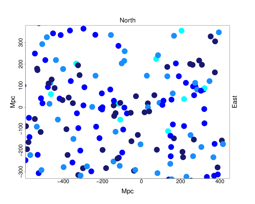
(a) The on-sky spatial coordinates of the absorbers in the GA and its immediate field, with colour-coding according to the four equivalent width (EW) bins of the $\lambda 2796$ Mg II line ($W_{r,2796}$). The four EW bins are divided: $0.0,0.3,0.6,1.0,10.0$ Å, with the lightest shades of blue representing the smallest values. There are more strong Mg II absorbers on the LHS (lower RA) of the GA than the RHS. Also there appears to be a tendency for the strong Mg II absorbers in the GA to clump into groups of a few.

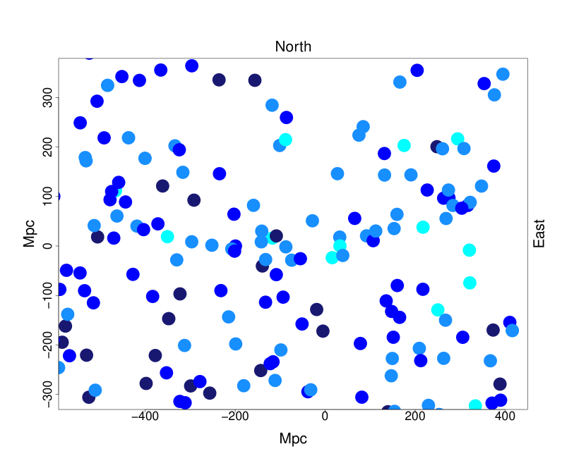
(b) The on-sky spatial coordinates of the absorbers in the GA and its immediate field, with colour-coding according to the four $i$ magnitude bins of the background quasars (probes). The $i$ bins are divided: $16.0,17.8,18.7,19.6,21.0$, with the lightest shades of blue representing the smallest values (this means that the lightest shade thus represents the brightest quasars). There appear to be more bright quasars on the RHS (higher RA) of the GA than the LHS.

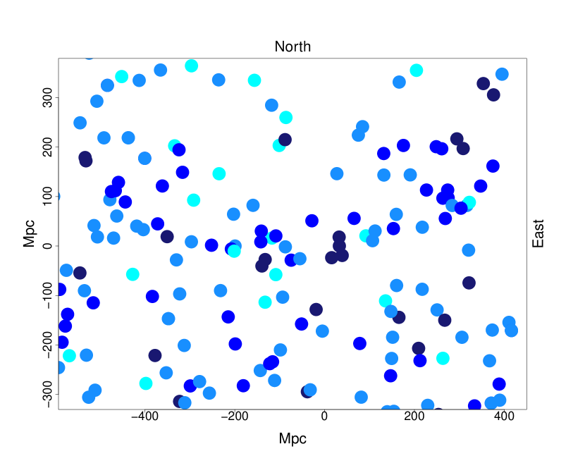
(c) The on-sky spatial coordinates of the absorbers in the GA and its immediate field, with colour-coding according to the four signal-to-noise (S/N) bins of the $\lambda 2796$ Mg II line. The four S/N bins are divided: $0,3,6,12,37$, with the lightest shades of blue representing the smallest values. By comparing Fig. 2(a) with the figure here, one will notice that the two properties are correlated.

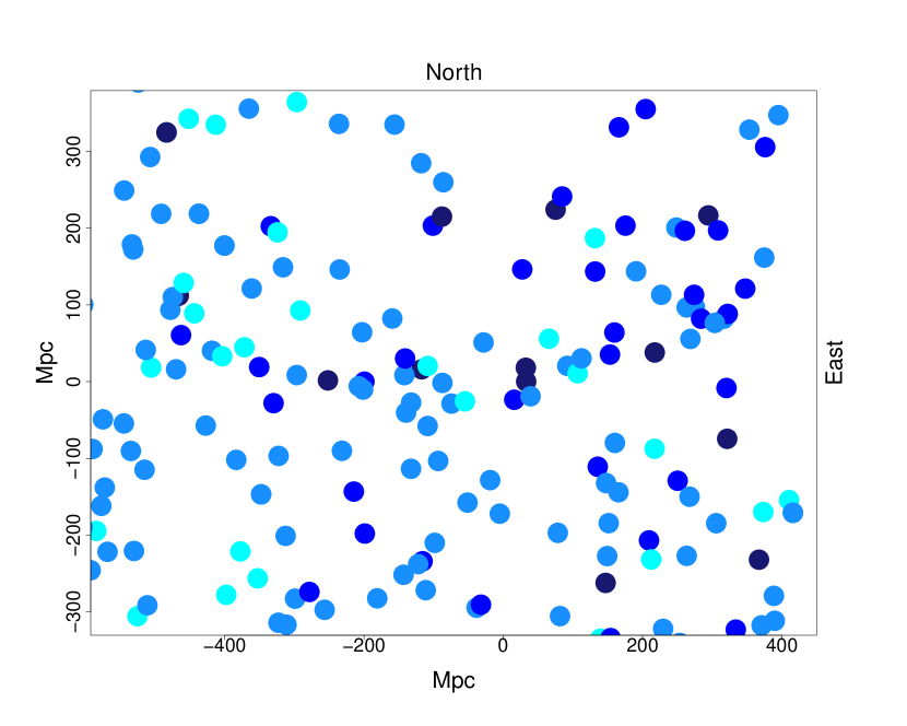
(d) The on-sky spatial coordinates of the absorbers in the GA and its immediate field, with colour-coding according to the four signal-to-noise (S/N) bins of the quasar continuum. The four S/N bins are divided: $0,8,16,24,47$, with the lightest shades of blue representing the smallest values. By comparing Fig. 2(b) with the figure here, one will notice that the two properties are correlated.

Figure 2: The on-sky spatial coordinates of the absorbers in the GA and its immediate field, with colour-coding according to the distribution of: equivalent width (EW) of the Mg II $\lambda 2796$ line ($W_{r,2796}$); quasar brightness ($i$); signal-to-noise (S/N) of the $\lambda 2796$ Mg II line; S/N of the quasar continuum. The lightest shades of blue represent the smallest values (for $i$, this means that the lightest shades represent the brightest quasars).

The EW of the $\lambda 2796$ Mg II line should correlate with the S/N of the $\lambda 2796$ Mg II line; Figs 2(a) and 2(c) show that this is indeed the case. The brightness ($i$) of the background quasar should correlate with the S/N of the quasar continuum; Figs 2(b) and 2(d) show that this is indeed the case. Note that brighter quasars, having a higher continuum S/N, can detect absorbers to a lower threshold EW.

An asymmetry is apparent in the distribution of Mg II EWs within the GA: the EWs tend to be stronger on the LHS (lower RA), and in the centre of the GA, than on the RHS (higher RA). Conversely, there is a tendency for the RHS to have brighter probes and higher continuum S/N, so, on the RHS, the threshold EW for detection should tend to be lower and certainly able to detect stronger absorbers, should they be present. Thus, the collected observations are consistent with the reality of the observed asymmetry of stronger absorbers on the LHS.

As discussed earlier, in Section 1.2, there have been many attempts to understand the relationship between EW and galaxy properties (morphology, luminosity, impact parameter, galaxy inclination etc.), but so far without a clear understanding of the connections between them. Conceivably, the asymmetry in the EW distribution could arise from the details of the geometry of the GA and the orientations of the galaxies within it. Future sky surveys and targeted observations seem likely to be necessary for progress on these details.

We note that there appears to be a preference for the strongest ($W_{r,2796}$) Mg II absorbers in the GA to clump together into groups of a few. See the dark blue points in Fig. 2(a), and note in particular those on the LHS of the GA (lower RA), the centre of the GA, and the group just above the tip of the RHS (higher RA) of the GA. As the GA is denser than the rest of the field, we can speculate that the occurrence of the strongest EWs in proximity is not accidental but is connected with the origin and environment of the GA.

Recall that the SZ cluster B18, $z=0.763$ (Burenin et al., 2018), is at the centre of the GA. (It is what led to the discovery of the GA.) At the centre of the GA is a small, circular ‘hole’, and surrounding this hole is a group of the stronger absorbers. SZ clusters create a highly-ionised environment, but Mg II absorption occurs in low-ionised regions. Possibly, a region of high ionisation can account for the hole, but an origin, in environment, of the enveloping group of stronger absorbers is not then obvious.

The investigation of small ($\Delta z=0.030$), overlapping (by 50 per cent) redshift slices reveals a noticeable difference between the left and right hand sides of the GA. For example, the LHS (lower RA) of the GA appears concentrated in the small redshift slice located farthest away ($z=0.832\pm 0.030$), whereas the RHS (higher RA) of the GA appears spread diffusely through the larger redshift slice. Interestingly, the LHS of the GA has both a narrower redshift distribution and a preference for stronger Mg II EWs.

Finally, the investigation of the redshift distribution suggests that, if the GA is represented as a segment of a cylindrical shell, then the LHS would be tilted away along the line of sight. That is, if the GA can indeed be represented as a segment of a cylindrical shell, then it is not precisely orthogonal to the line-of-sight but is rotated with respect to a north-south axis.

2.3 Connectivity and statistical properties

The GA was discovered visually, from a Mg II density image (e.g. Fig. 1). Albeit after the event, we now discuss its connectivity and statistical properties. The Mg II absorbers can, of course, be found only where there are background quasars to act as probes, and those probes may themselves be subject to spatial variations arising from large-scale structure and, in particular, from artefacts in the surveys.

We apply three different statistical methods for assessing the GA, as follows.

(i) SLHC / CHMS — see Clowes et al. (2012). This method depends first on constructing the 3D minimal spanning tree (MST), and then separating it at some specified linkage scale. At this stage it is equivalent to single-linkage hierarchical clustering (SLHC). The statistical significance of a candidate structure is then assessed using its volume obtained as the volume of the ‘convex hull of member spheres’ (CHMS). Note the important feature that this method assesses the significance of individual candidate structures.

(ii) The Cuzick-Edwards (CE) test — see Cuzick & Edwards (1990). It is a 2D ‘case-control’ method that is designed to correct the incidence of cases for spatial variations in the controls (the underlying population). It depends on the number of cases that occur within the $k$ nearest neighbours. The CE test can detect the presence of clustering in the field, while correcting for variations in the background, and can assess its statistical significance. It cannot, however, assess the physical scale of the clustering.

(iii) 2D Power Spectrum Analysis (2D PSA) — see Webster (1976a). It is a powerful Fourier method for detecting clustering in the field. It can be effective even for detecting weak clustering. The 2D PSA can detect the scale of clustering and assess the statistical significance of the clustering at that scale.

Each of these tests has distinctive attributes, and the reader should judge the evidence provided by the ensemble. Only the SLHC / CHMS method assesses the significance of individual candidate structures, whereas the CE test and the 2D PSA address clustering in the field. We shall describe below the ‘polygon approach’, in which we assess the contribution that the GA makes to the results from the CE test and the 2D PSA for the field. Only the CE test can correct for spatial variations in the underlying population. However, we shall describe below, again using the polygon approach, that the 2D PSA has more power to discriminate than the CE test.

Finally, we emphasise again, that given the nature of the discovery the statistical analysis is necessarily performed post-hoc. The reader will find that we have used techniques to compare the field containing the GA with other, unrelated fields (within the same Mg II dataset). This of course has its limitations due to the non-uniformity of the background quasars (probes) and potential survey artefacts. We have also compared with randomised simulations, in which we attempt to preserve these subtleties of the Mg II data.

2.3.1 SLHC / CHMS (Minimal Spanning Tree)

The minimal spanning tree (MST) is a widely-used algorithm for assessing large-scale structure in astronomy and cosmology. When the MST is separated at some specified linkage scale it is equivalent to the algorithm for single-linkage hierarchical clustering (SLHC). An approach to assessing the statistical significance of the agglomerations found in this way was introduced by Clowes et al. (2012): the Convex Hull of Member Spheres (CHMS) method. It was further used by Clowes et al. (2013) in the analysis of the Huge-LQG, the Huge Large Quasar Group that they discovered.

Here, we apply the sequence of SLHC and CHMS to the Mg II absorbers in the GA field. By specifying a linkage scale and a minimum membership, the SLHC identifies the 3D agglomerations or groups within the coordinates of the absorbers. Within each identified group the CHMS constructs a sphere around each member point with a radius of half the mean linkage separation for that group. A volume for the group is then computed as the volume of the convex hull of its member spheres (and note that the convex hull is a unique construction). An expected density of absorbers is determined from a control field and the observed redshift interval of a group. (Here, the control field is specified as the same field that is being assessed.) The observed number of member points within a group are then scattered randomly within a cube at the expected density, and their CHMS volume is calculated; this is done 1000 times. The significance of the group is calculated by the rate of occurrence of randomly-generated CHMS volumes that are smaller than the observed volume. See Clowes et al. (2012) for full details of the CHMS method.

In principle, this SLHC / MST approach should be applied only to surveys that have no intrinsic spatial variations. The background quasars — the probes of the Mg II absorbers — are drawn from a merger of the SDSS DR7QSO and DR12Q databases. While a reasonably spatially-uniform subset can be extracted from DR7QSO, DR12Q is much more strongly affected by spatial artefacts arising from deeper areas. Thus the distribution of the background quasars can conceivably affect the distribution of the Mg II absorbers in some, possibly complicated, way. However, if the distribution of the background quasars appears to be reasonably homogeneous in the area of interest, then we can assume that the distribution of Mg II absorbers is predominantly a product of the LSS and not the availability of background quasars. Of course, the distribution of background quasars can still have some effects — such as occasional gaps in connectivity — on the Mg II absorbers even in such reasonably homogeneous regions.

Fig. 3 shows the kernel-smoothed distribution ($\sigma=11$ Mpc, present epoch) of the background probes (quasars) in the area of the GA for $z>0.862$. It is clear that there are denser areas, less dense areas, and even empty patches, across the whole image, indicating the spatial non-uniformity of the background probes. There is a particularly dense band in approximately the northern third, which arises from a deeper area of the DR12Q survey. However, there are evidently no artefacts that correspond to the dimensions and orientation of the GA.

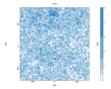
Figure 3: The tangent-plane distribution of background probes (quasars) in the GA field with redshifts $z>0.862$, represented by the dark blue points. The blue contours, increasing by a factor of two, represent the density distribution of the quasars using a Gaussian kernel with a smoothing scale of $\sigma=11$ Mpc. The axes are labelled in Mpc, scaled to the present epoch. East is towards the right and north is towards the top. It is clear that there are denser areas, less dense areas, and even empty patches, across the whole image, indicating the spatial non-uniformity of the background probes. There is a particularly dense band in approximately the northern third. However, there are evidently no artefacts that correspond to the dimensions and orientation of the GA.

We are now taking the GA to be predominantly concentrated in the redshift interval $0.802\pm 0.060$, so $0.742\rightarrow 0.862$. Its (present-epoch) depth is then $\sim 340$ Mpc.

This redshift interval appears to be the optimum, following a heuristic process of stepping through a range of redshift intervals and determining the membership and significance of the GA through the SLHC / CHMS method. Redshift intervals of thickness $\Delta z=\pm 0.050$ between $0.760<z<0.810$ were tested, using various linkage scales, and a clear peak signal for the GA was seen around the redshift $z=0.810$ using a linkage scale of $95$ Mpc. (See Section 2.3.2 for the details of choosing the optimum linkage scale.) Further, finer-scale, testing revealed the greatest number of connected GA members to be more precisely located at $z=0.802$, again for the linkage scale of $95$ Mpc. The significance for $z=0.802\pm 0.050$ is $4.15\sigma$. Widening the redshift interval to $z=0.802\pm 0.060$ gives a slightly higher significance of $4.30\sigma$, and the number of member Mg II absorbers is then increased from 42 to 44.

A second, smaller, agglomeration made up of 10 and 11 absorber members at both $z=0.802\pm 0.050$ and $z=0.802\pm 0.060$ respectively, although not formally significant ($1.75\sigma$ and $2.04\sigma$ respectively), is clearly also part of what we identified visually as the Giant Arc. Conceivably, just one further background probe would be sufficient to yield one further absorber that would then connect both agglomerations as one significant unit. We have emphasised the limitations of the SLHC / CHMS method for this dataset, and we might here be seeing their consequences.

As noted above, the estimation of the CHMS significance requires a control field from which the expected average density is calculated. For the CHMS significances given above, we used the same field as that containing the GA. This was a deliberate choice, given the spatial variations of the wider survey. Clearly, the GA must then represent a small fraction of the total area and number of absorbers ($\sim$ 7 per cent of the absorbers are from the GA).

Even so, the distribution of background probes (quasars) in the field of the GA is not uniform — notably the denser band in the northern third. This non-uniformity could affect the CHMS calculations of significance, either by overestimating or underestimating, depending on whether the probes are generally under-populated or over-populated in the control field. A second estimate of the significance can be calculated from the CHMS method by increasing the field-of-view (FOV) containing the GA, and using it as a new control field. Fig. 4 shows the background probes in the field containing the GA with the western and southern boundaries extended. Note that the eastern and northern boundaries were not extended because of proximity to the edge of the survey area.

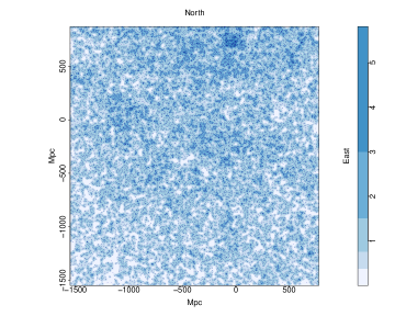
Figure 4: The tangent-plane distribution of background probes (quasars), in the same region of sky as the GA for redshifts $z>0.862$, represented by the dark blue points. The field-of-view has here been increased by extending the western and southern boundaries. The blue contours, increasing by a factor of two, represent the density distribution of the quasars using a Gaussian kernel with a smoothing scale of $\sigma=11$ Mpc. The axes are labelled in Mpc, scaled to the present epoch. East is towards the right and north is towards the top.

Using the larger FOV in the redshift interval $z=0.802\pm 0.060$, the CHMS method calculates a significance of $4.53\sigma$ for the principal agglomeration of the GA. As noted previously, the GA is split into two agglomerations by the SLHC algorithm, shown in Fig. 5. For this entire, larger, FOV, there are 35 agglomerations in total, with the principal agglomeration of the GA being the largest and most significant, and the only agglomeration with a significance $>3.5\sigma$. Fig. 5 shows the GA as located by the SLHC / CHMS method, with the principal agglomeration represented by the black points; the red points indicate the smaller, separate agglomeration of much lower significance, but visually it can clearly be seen as part of the GA.

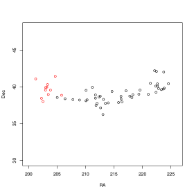
Figure 5: The GA connected via the SLHC algorithm. There are 44 black points which indicate the principal agglomeration of the Giant Arc — the largest, and most significant agglomeration in the field —, which comprises the majority of the GA. There are 11 red points which indicate the secondary agglomeration of the GA, which, although by itself not statistically significant, is clearly part of the GA. The axes are labelled RA and Dec where east is towards the right and north is towards the top.

The SLHC / CHMS algorithm is next applied to three lower redshift slices — $z=0.682\pm 0.060$, $z=0.562\pm 0.060$, and $z=0.442\pm 0.060$ — in the same (larger) FOV as the GA (see Fig. 4). Using lower redshift slices and the same FOV means that we can conveniently compare the Mg II absorbers arising from the same probes as those in the GA field by restricting the probes to $z>0.862$. We can also apply the SLHC / CHMS method to the same three lower redshift slices without this redshift restriction on the probes. Recall, however, that the probes may show density artefacts with a large FOV. As mentioned previously, the SLHC / CHMS method can be problematic for the Mg II analysis because of these artefacts. Therefore, superficially significant structures that correspond to particularly dense patches of probes are likely to be discarded. The results are summarised in Table LABEL:tab:zslices_list.

As can be seen in Table LABEL:tab:zslices_list there are significant ($\sim 3\sigma$) structures. At a more cautious limit of $4\sigma$, however, there were only two candidate structures which did not reside in an artefact (in redshift slices $z=0.682$ and $z=0.562$). We shall in due course investigate them further, starting with optimisation of the redshift intervals.

Finally, we introduce a random-simulation aspect to the SLHC / CHMS analysis. We have carried out 1000 random simulations as follows. (i) We consider the large, extended area that corresponds to (Fig. 4). (ii) We consider only the probes at higher redshift than the redshift slice of the GA — that is, we continue (as with the slices of redshift lower than that of the GA) to use only the probes appropriate to the GA, so that density artefacts in the probes remain identical. (iii) We reassign at random MgII absorbers of any redshift to the probes, while not splitting occurrences of multiple absorbers per line of sight. (Note that splitting absorbers would have the undesirable effect of changing the total number of probes with absorbers.) (iv) We then analyse the random-simulated data as for the actual GA slice, selecting absorber redshifts for the redshift slice.

Within the simulations, we looked for “structures” that had properties comparable to, or more extreme than, the observed properties of the GA (precisely, of GA-main — see below). The properties considered were the set of: number of members; SLHC / CHMS significance; and overdensity. In all cases (roughly one occurrence per two simulations), we found that these “comparable structures” were in the regions of the visually-obvious density artefacts, and never in the region occupied by the real GA. The occurrence of the “comparable structures” in the density artefacts is as expected: for those artefacts, the linkage scale and the control density would clearly not be appropriate. We can infer that the probability of the real GA (precisely, GA-main) occurring as a random event is $<0.001$.

The SLHC algorithm easily identifies the GA, with 44 connected Mg II absorbers, and the CHMS method estimates a significance of $\sim 4.5\sigma$ using the central redshift $z=0.802$. In every redshift interval investigated, the GA appears in two parts: (i) the principal agglomeration, which is large in both physical size and membership, and statistically very significant; and (ii) the secondary agglomeration, small in size and membership, and by itself statistically not significant. As mentioned earlier, the Mg II absorbers depend on the availability of background probes (quasars), and without those, Mg II would not be detected. Thus an artefact in the distribution of probes — i.e. a gap, perhaps of just one missing probe — could lead to an artefact of apparent splitting into two agglomerations.

We have seen previously, in Section 2.2, that there is a noticeable difference between the LHS and RHS of the GA with regards to redshift distribution. Investigating small ($\Delta z=0.030$), overlapping (by 50 per cent) redshift slices has highlighted the sub-structure of the GA along the redshift axis. We find that the larger agglomeration of the GA is distributed more evenly and widely along the redshift axis, while the smaller agglomeration is concentrated in a narrower redshift slice. It becomes clear from the central redshift slice and below ($z<0.802$) that there are no Mg II absorbers available that can connect the small agglomeration to the large agglomeration.

More data, such as the new SDSS DR16Q quasar database (Lyke et al., 2020), could provide additional information to investigate the GA further. This includes, conceivably, the possibility of connecting the small agglomeration to the large agglomeration of the GA. However, this would require construction of a new Mg II catalogue corresponding to the DR16Q quasars. In the future, we plan to create our own Mg II catalogues from previous and future quasar data releases.

2.3.2 Selecting a Linkage Scale

The linkage scale that is set in the SLHC / CHMS method determines both the number of agglomerations and their memberships. It was set at $95$ Mpc for the GA. This setting was partly guided by the linkage scale that was known to be effective for the CCLQG, and which, when used subsequently, led to the discovery of the Huge-LQG and many other LQGs (see Clowes et al. (2012) and Clowes et al. (2013)). Clearly, the linkage scale must be adjusted for field density; in this case, starting from the linkage scale that was effective for LQGs (i.e. for LSS in quasars) we calculate a linkage scale of $85$ Mpc for Mg II absorbers in the GA field. From here we followed the heuristic process described in Section 2.3.1 to identify an optimum linkage scale of $95$ Mpc for the Mg II absorbers.

One must remember that Mg II absorbers are distinctly different from quasars and therefore cannot be treated in quite the same way. For example, the linkage scale that works for quasars will not necessarily work for the Mg II absorbers since the latter is a case of inhomogeneities (the absorbers) superimposed on inhomogeneities (the quasars and survey artefacts). Future work will address the development of a clustering analysis that is specifically addressed to the requirements of Mg II absorbers.

It is in the nature of discoveries that there will be a post-hoc aspect to the analysis. What turned out to be effective for the CCLQG led to the discovery of the Huge-LQG: an initial discovery, followed by a heuristic process, followed by an entirely objective a-priori new discovery. It is in this spirit that we present the discovery of the GA: one for which the techniques and parameters used to assess and characterise it can subsquently be applied to the whole Mg II database.

For completeness, we can briefly mention what results from instead setting the linkage scale to $85$ Mpc, $90$ Mpc, $100$ Mpc, and $105$ Mpc for the adopted redshift slice. In five runs, using linkage scales of $85$ Mpc, $90$ Mpc, $95$ Mpc, $100$ Mpc, and $105$ Mpc, there are totals of $4$, $25$, $35$, $43$, and $3$ agglomerations found respectively, with the GA always being the most significant in all except the $105$ Mpc run. The middle three runs split the GA into two parts — one large and significant, and one smaller and less significant. For the following comments, we concentrate only on the large, significant part of the GA located in the middle three runs ($90$, $95$ and $100$ Mpc), which makes up the majority of what we visually identified as the GA. (1) It has a significance greater than $3.8\sigma$ in all of the three runs. (2) It is the only agglomeration that has a significance greater than $3.5\sigma$, with only two or three agglomerations above $3\sigma$ (all others being below a $3\sigma$ threshold). (3) In both the $90$ Mpc and $95$ Mpc runs, it is the largest agglomeration by membership, and is the second largest by membership in the $100$ Mpc run. Lastly, we mention what arises from setting the linkage scale to $85$ Mpc and $105$ Mpc. Using these linkage scales one can see that the SLHC / MST method has reached its maximum and minimum limit with the linkage scales, as there are only $4$ and $3$ structures found, respectively. The corresponding memberships are $20$ and $133$ with significances of $3.6\sigma$ and $0.8\sigma$, respectively. As is demonstrated, going any lower or higher with the linkage scale would yield nothing of consequence: either no structures, or one large structure containing almost everything. It is worth noting that, although the $85$ Mpc linkage scale is the minimum at which structures can be found in the Mg II data at this redshift / density, the GA is still mostly detected, still the largest agglomeration in the field, and the only structure detected with a significance over $3\sigma$ — see Fig. 6

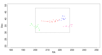
Figure 6: The four structures found via the SLHC / CHMS method using a reduced linkage scale of $85$ Mpc. The black dashed rectangle corresponds to Fig. 5 for comparison. The GA is still mostly detected in what appears to be two parts. The largest agglomeration, containing $20$ Mg II absorber members represented by the red points in the figure, makes up the majority of what we visually identify as the GA. The second largest agglomeration, containing $14$ Mg II absorber members represented by the blue points in the figure, is also part of what we visually identified as the GA and can be seen as an extension of the red points. The axes are labelled RA and Dec where east is towards the right and north is towards the top.

Note that for future work, involving the remainder of the Mg II database, we can adopt this scale of $95$ Mpc as a standard, with scaling according to the density of absorbers (i.e., $s=(\rho_{0}/\rho)^{1/3}s_{0}$) in the volumes of interest.

2.3.3 Cuzick-Edwards test

We mentioned above that, strictly, the SLHC / MST approach should be applied only to surveys that have no intrinsic spatial variations. However, a statistical test for (two-dimensional) clustering exists that is designed to manage spatial variations in the source data: the Cuzick-Edwards test (Cuzick & Edwards, 1990). We apply it here.

The Cuzick-Edwards test (hereafter CE test) has been used mainly in medical research, such as the clustering patterns of diseases within unevenly populated geographical regions. (The essential character of our problem is the same.) It adopts a ‘case-control’ approach to a $k$ nearest-neighbour (NN) analysis. Several papers have compared the properties of the CE test amongst various spatial clustering analyses and assert that the CE test is powerful and sensitive in estimating clustering significance within a point dataset — see, for example, Song & Kulldorff (2003), Meliker et al. (2009) and Hinrichsen et al. (2009). In Song & Kulldorff (2003) the authors note that the CE test is used more appropriately if the level of clustering is known beforehand.

Inevitably, for our problem, the statistical properties of the GA are tested after the event of discovery (i.e. the level of clustering is known).

We used the CE test that is coded in the application qnn.test in the R package smacpod (French, 2020) — Statistical Methods for the Analysis of Case-Control Point Data. The probes (i.e. the background quasars) are labelled as ‘controls’ and the Mg II absorbers in the redshift interval are labelled as ‘cases’. The qnn.test then uses a NN algorithm to find the $q$ (or $k$) NNs of any case to another case.

The test statistic is then calculated as

$$T_{k}=\sum_{i=1}^{n}\delta_{i}d_{i}^{k}$$

where
$\delta_{i}=1$ if the data point is a case or $0$ if it is a control;
$d_{i}^{k}=1$ if the NN is a case and $0$ if it is a control.

The $p$-value from qnn.test is calculated from simulations under the random-labelling hypothesis (French, 2020) for $\mathrm{nsim}=2000$ simulations.

The choice of maximum $q$ ($k$) value that is adopted for the test will depend on the control-case ratio, as can be seen from the test statistic calculation. There are $\sim 20$ times as many probes (controls) as Mg II absorbers (cases) in the redshift interval of the GA. Cuzick & Edwards (1990) examine the power of the CE test with varying control-case ratios and find that a control-case ratio of between $4$ and $6$ is optimum (see their Fig. 5).

Therefore, we choose to use a control-case ratio of $\sim$ 5:1. To achieve this we randomly select 25 per cent of the probes, for each of 100 runs of qnn.test. (Randomly-selected controls that duplicate the coordinates of the cases in a given run are removed.) The 100 runs also allow us to assess how robust are the estimates of significance for the Mg II absorbers.

We use a set of $q$ ($k$) values: 1, 2, 4, 8, 12, 16, 20, 24, 28, 32, 36, 40, 44, 48, 52, 56, 60, and 64. We start by applying the qnn.test to the basic GA field.

Then, to assess the (presumed) dominance of the GA itself we apply the test to a succession of smaller fields (smaller in the north-south direction), all centred on the GA. In Figs 7 to 9, the median $p$-value over 100 runs of 2000 random simulations is shown plotted against the chosen $q$ values, with the corresponding flat-fielded Mg II image shown alongside.

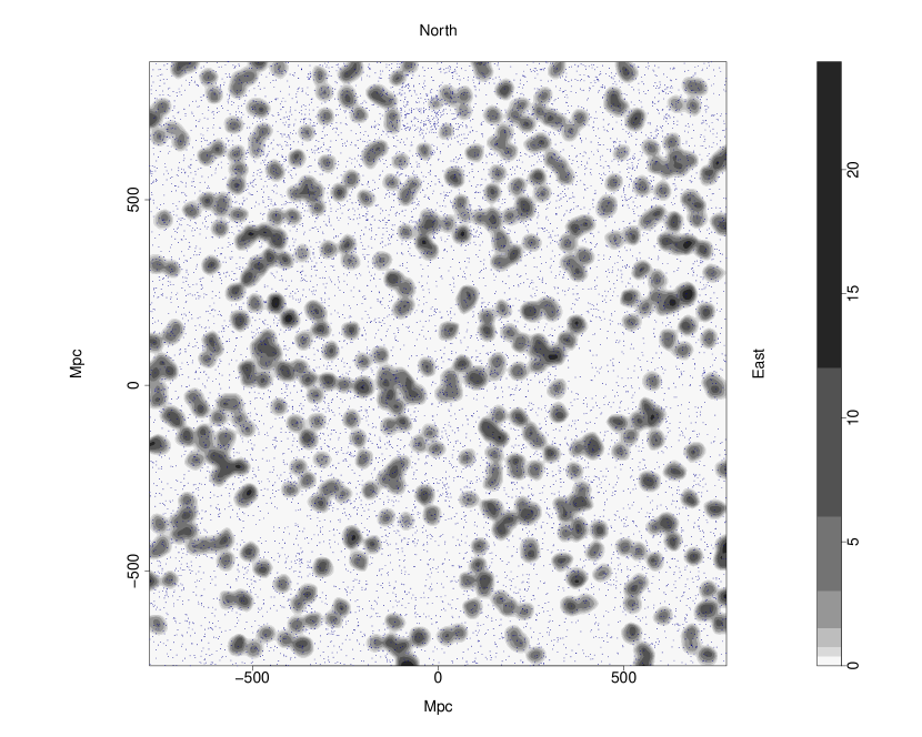
(a) Density distribution of the flat-fielded Mg II absorbers represented by the grey contours which have been smoothed using a Gaussian kernel of $\sigma=11$ Mpc and increase by a factor of two. Blue dots represent the background probes (quasars).

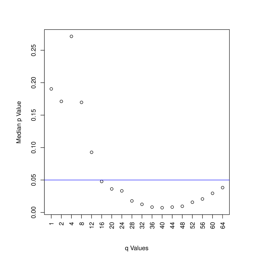
(b) The median $p$-value over 100 runs of 2000 simulations as a function of chosen $q$ ($k$) value in the GA field; see the adjacent image. The blue, horizontal line is set to $p=0.05$. The $p$-value is at a minimum of $0.0072$ when $q$ is $40$.

Figure 7:

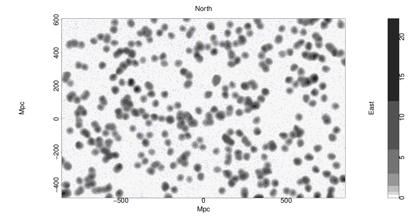
(a) Density distribution of the flat-fielded Mg II absorbers represented by the grey contours which have been smoothed using a Gaussian kernel of $\sigma=11$ Mpc and increase by a factor of two. Blue dots represent the background probes (quasars). This is the first ‘zoom’ of the GA, where the GA field has been reduced in the north and south boundaries.

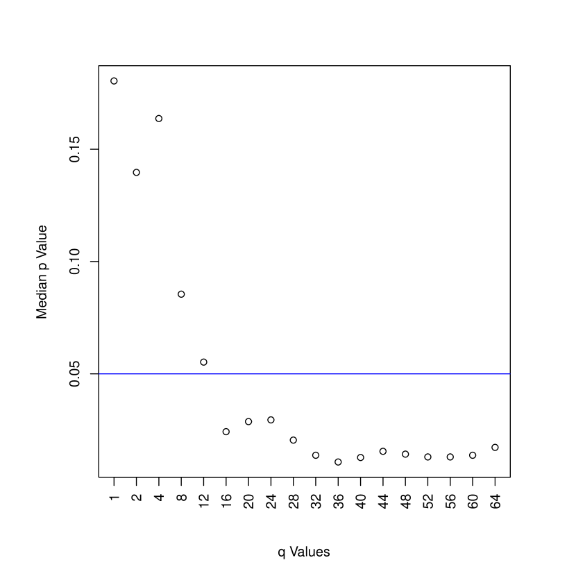
(b) The median $p$-value over 100 runs of 2000 simulations as a function of chosen $q$ ($k$) value in the first ‘zoomed’ field containing the GA; see the adjacent image. The blue, horizontal line is set to $p=0.05$. The $p$-value is at a minimum of $0.0107$ when $q$ is $36$.

Figure 8:

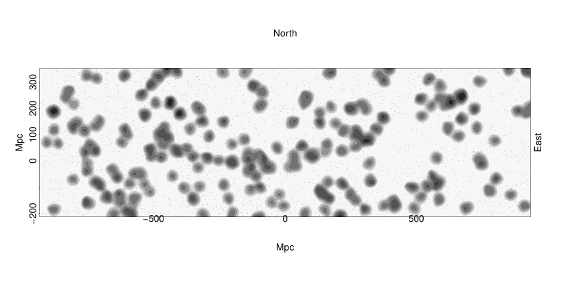
(a) Density distribution of the flat-fielded Mg II absorbers represented by the grey contours which have been smoothed using a Gaussian kernel of $\sigma=11$ Mpc and increase by a factor of two. Blue dots represent the background probes (quasars). This is the second ‘zoom’ of the GA, where the GA field has been further reduced in the north and south boundaries.

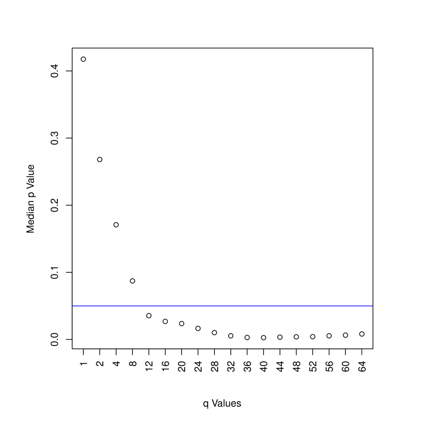
(b) The median $p$-value over 100 runs of 2000 simulations as a function of chosen $q$ ($k$) value in the second ‘zoomed’ field containing the GA; see the adjacent image. The blue, horizontal line is set to $p=0.05$. The $p$-value is at a minimum of $0.0027$ when $q$ is $40$.

Figure 9:

The process of zooming into the GA allows the GA to become the dominating feature in the field, which, as a result, increases the significance of clustering (i.e. smaller $p$-value). In the first Mg II field, Fig. 7(a), the minimum $p$-value is $0.0072$ at a $q$-value of $40$, which (assuming a normal distribution) is equivalent to a significance of $\sim 2.68\sigma$, Fig. 7(b). Whereas in the third Mg II field, Fig. 9(a), the minimum $p$-value drops to $0.0027$ at a $q$-value of 40, which is equivalent to a significance of $3.00\sigma$, Fig. 9(b). In this way we can judge that the GA is the dominant, contributing factor to the significant level of clustering in the field.

The heuristic process of ‘zooming’ into the GA was next applied to three other fields at lower redshift slices ($z$: $0.682$, $0.562$, $0.442$) centred on the sky coordinates of the GA. The background probes are kept the same in the three new fields as those in the GA field, allowing a direct comparison of clustering in just the Mg II absorbers (as in Section 2.3.1). Figs 10 to 12 show the results of the CE test for the three lower redshift fields using the smallest field size (i.e. the second ‘zoom’). The $p$-value profiles as a function of $q$-value in each of the lower redshift fields appear more scattered and varied compared with the GA results.

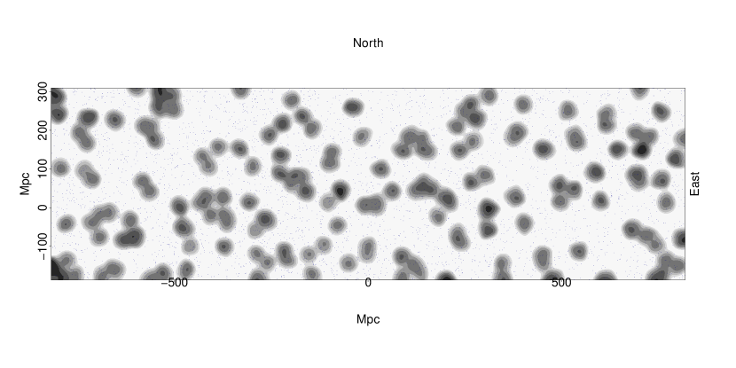
(a) Density distribution of the flat-fielded Mg II absorbers in the redshift interval $z=0.682\pm 0.060$, on the same sky coordinates of the ‘zoomed’ GA field, represented by the grey contours which have been smoothed using a Gaussian kernel of $\sigma=11$ Mpc and increase by a factor of two. Blue dots represent the background probes (quasars).

(b) The median $p$-value over 100 runs of 2000 simulations as a function of chosen $q$ ($k$) value in the $z=0.682\pm 0.060$ redshift interval on the same sky coordinates as the ‘zoomed’ GA field; see the adjacent image.

Figure 10:

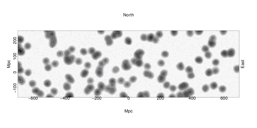
(a) Density distribution of the flat-fielded Mg II absorbers in the redshift interval $z=0.562\pm 0.060$, on the same sky coordinates of the ‘zoomed’ GA field, represented by the grey contours which have been smoothed using a Gaussian kernel of $\sigma=11$ Mpc and increase by a factor of two. Blue dots represent the background probes (quasars).

(b) The median $p$-value over 100 runs of 2000 simulations as a function of chosen $q$ ($k$) value in the $z=0.562\pm 0.060$ redshift interval on the same sky coordinates as the ‘zoomed’ GA field; see the adjacent image.

Figure 11:

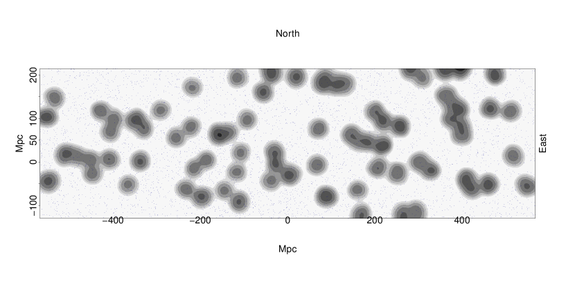
(a) Density distribution of the flat-fielded Mg II absorbers in the redshift interval $z=0.446\pm 0.060$, on the same sky coordinates of the ‘zoomed’ GA field, represented by the grey contours which have been smoothed using a Gaussian kernel of $\sigma=11$ Mpc and increase by a factor of two. Blue dots represent the background probes (quasars).

(b) The median $p$-value over 100 runs of 2000 simulations as a function of chosen $q$ ($k$) value in the $z=0.446\pm 0.060$ redshift interval on the same sky coordinates as the ‘zoomed’ GA field; see the adjacent image.

Figure 12:

The major difference between the $p$-value profiles for the GA field and the $p$-value profiles for three lower redshift fields is that there is no sign of any significant results ($p$-value $<0.05$) in any of the three lower redshift fields for any of the chosen $q$-values. The background probes were the same in all four fields (GA field and the three lower redshift fields) indicating that the Mg II absorbers are responsible for the different $p$-value profiles. From this we can assert that the GA field is markedly distinct, with significant clustering attributable to the GA.

As a further test of the dominance of the GA in the CE statistics we have applied our ‘polygon-approach’. Visually, we draw a polygon around what we identify visually as the member absorbers of the GA. We leave the absorbers in the polygon untouched but reassign (i.e. shuffle) at random the $y$-coordinates of absorbers outside the polygon, while avoiding the area within the polygon. We apply this process to the data of Fig. 9(a). In this way we can compare the CE statistics arising from the original data with those in which the GA points inside the polygon are unchanged but those outside the GA polygon are randomised. We find that the range of $p$-values for the original data ($p$-values $\sim$ 0.002–0.003) is very similar to that of the GA $+$ randomised data ($p$-values $\sim$ 0.001–0.003), suggesting that the GA is indeed the dominant source of the clustering signal.

2.3.4 Power Spectrum Analysis

Power Spectrum Analysis (PSA) — see mainly Webster (1976a), but also Webster (1976b) and Webster (1982) — is a powerful Fourier method for assessing the presence and significance of clustering in rectangular (2D PSA) or cuboidal fields (3D PSA). PSA was designed to be effective for the detection of clustering that may be weak and escape detection by other methods; it is, however, not a case-control method. A brief summary of the theory of PSA may be found in section 5 of Clowes (1986).

We apply 2D PSA to the same rectangular field, illustrated in Fig. 9(a), that was used for the CE analysis above. Fig. 13 shows the plot of the intermediate PSA statistic $Q^{\prime}$ against $1/\lambda$. The (six) high points towards the left of the plot allow a clustering scale of $\lambda_{c}\sim 270\,\mathrm{Mpc}$ to be identified. The final PSA statistic $Q$ for this scale $\lambda_{c}$ corresponds to a detection of clustering at a significance of $4.8\sigma$.

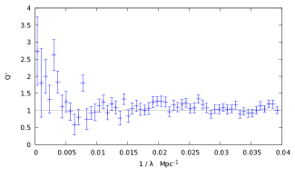
Figure 13: The plot shows the PSA statistic $Q^{\prime}$ plotted against $1/\lambda$, with $\lambda$ in Mpc, for the 2D PSA. The bin size is $6.7\times 10^{-4}\,\mathrm{Mpc^{-1}}$ and the error bars are $\pm\sigma$. The horizontal line $Q^{\prime}=1$ indicates the expectation value in the case of no clustering. The (six) high points towards the left of the plot allow a clustering scale of $\lambda_{c}\sim 270\,\mathrm{Mpc}$ to be identified. The final PSA statistic $Q$ for this scale $\lambda_{c}$ corresponds to a detection of clustering at a significance of $4.8\sigma$.

We have applied the polygon-approach here also. As in the discussion above for the CE method, we leave the GA absorbers in the polygon untouched but reassign (i.e. shuffle) at random the $y$-coordinates of absorbers outside the polygon, while avoiding the area within the polygon. In this way we can establish that the significance from the 2D PSA of the GA absorbers alone — i.e. with other absorbers randomised — has a mean value $\sim 3.5\sigma$ (with a range 3.0–4.4$\sigma$) for the original scale $\lambda_{c}\sim 270\,\mathrm{Mpc}$. In fact, the value of $\lambda_{c}$ for the polygon-approach varies too, with the mean significance at the actual values of $\lambda_{c}$ being $\sim 3.8\sigma$.

From this polygon-approach, it appears likely that, while the GA is the dominant contributor to the PSA result, a smaller contribution from other absorbers in the field is detected too. This outcome might be expected, given the power of the PSA method. The failure to detect a contribution from the other absorbers with the CE method could be because the CE method is intrinsically less sensitive, or because its case-control correction has successfully eliminated artefacts from the background probes (the controls).

The polygon-approach can also be used to assess the relative power of the 2D PSA and the CE test. For example, we reduced the number of GA absorbers in the polygon from 52 to 42 by random selection (with the points outside the polygon being randomised as usual but unchanged in total number). In that case, the GA is generally not detected by the CE test, at a significance level of 0.01 ($2.3\sigma$), but is generally still detected by the PSA, at $>2.7\sigma$. The power of a statistical test to discriminate is an important factor, and an uninteresting $p$-value does not necessarily mean nothing interesting in the data. Webster (1976a) demonstrates that the PSA has more power to detect clustering than a simple nearest-neighbour test. The CE test uses multiple neighbours, and so can be expected to have more power than a nearest-neighbour test, but, as our tests with the polygon-approach suggest, still has less power than the PSA. Of course, the CE test has the useful feature of case-control comparisons, whereas the PSA does not.

2.4 Overdensity

As seen previously, the SLHC / CHMS method splits the GA into two agglomerations - one large, statistically significant portion which makes up the majority of what we visually identified as the GA, and one smaller, statistically not significant portion which makes up the remainder of what we visually identified as part of the GA. We will refer to these agglomerations as GA-main and GA-sub, respectively, for simplicity. The overdensity of the GA can be calculated using the CHMS approach as described earlier in the paper (section 2.3.1). However, in the case of a strongly curved structure such as the GA (and GA-main), the MST-based method of Pilipenko (2007) can have some advantages. We shall refer to these two methods as CHMS-overdensity and MST-overdensity, respectively. The MST-overdensity does not consider the physical volume of the structure being assessed. Instead, it calculates the overdensity based on the MST edge-lengths: $\delta=\langle l_{0}^{3}\rangle/\langle l^{3}\rangle-1$ where $l$ is MST edge-length for the structure and $l_{0}$ is that for a control field. Given the curvature of GA-main, the CHMS volume and CHMS-overdensity refer to a volume that encloses both GA-main and some space above it (where there are rather fewer absorbers, and those are not related to the GA). Therefore, the CHMS method is likely to overestimate the volume and underestimate the overdensity. In contrast, the MST-overdensity, which is an internal measure that considers only the points belonging to the group, and no additional space arising from curvature, is likely to be a better estimate of the overdensity. Conversely, GA-sub is a globular shape, so it is possible to construct a unique volume enclosing only the absorbers attached to GA-sub and not additional ones at lower density. Therefore, the CHMS-overdensity calculation for GA-sub is likely to be a fair estimate.

GA-main, as mentioned earlier, has a significance of $4.5\sigma$, while GA-sub has a much smaller significance of $2.3\sigma$. By splitting the usual control field (using the larger field-of-view, see Fig. 4) into eight portions — four quarter segments and four half segments — we repeatedly calculate the significance and the overdensities of GA-main and GA-sub using different control fields. An uncertainty can then be estimated for the significance and overdensities for both portions of the GA. Our results are as follows: (1) GA-main, containing 44 Mg II absorbers, has a significance of $(4.5\pm 0.6)\sigma$; a CHMS-overdensity of $\delta\rho_{CHMS}/\rho_{CHMS}=0.9\pm 0.6$; and an MST-overdensity of $\delta\rho_{MST}/\rho_{MST}=1.3\pm 0.3$; (2) GA-sub, containing 11 Mg II absorbers, has a significance of $(2.1\pm 0.9)\sigma$; a CHMS-overdensity of $\delta\rho_{CHMS}/\rho_{CHMS}=1.5\pm 0.3$; and an MST-overdensity of $\delta\rho/\rho=1.3\pm 0.3$. As expected, the CHMS-overdensity is lower than the MST-overdensity for GA-main, indicating that the CHMS unique volume encapsulating GA-main is likely to be an overestimate because of the curvature of the arc. In contrast, for GA-sub, which has a globular-shape, the CHMS-overdensity and the MST-overdensity have similar values, as expected when there is no marked curvature. In addition, the CHMS-overdensity has a much larger error than the MST-overdensity which suggests giving preference to the latter. Notice here that both GA-main and GA-sub have the same MST-overdensity, which supports their belonging to the same structure.

A final method of calculating the number overdensity is to simply draw a rectangle around the visually-selected Mg II absorbers in the GA and compare the number of absorbers per unit area in the rectangle to the number of absorbers in the whole field. The method will underestimate the GA overdensity for three reasons: (i) the GA contributes to the density of the whole field, although only by a small fraction; (ii) the rectangular shape around the GA overestimates the area encompassing the GA as the GA is curved, therefore having a large portion of ‘empty’ space (with non-GA absorber members); (iii) this method encompasses the whole GA from visual inspection, rather than separating it into two agglomerations like the CHMS method, thus reducing the overall density in the GA rectangle. Using this method we calculate an overdensity of $\delta\rho/\rho\sim 0.93$.

In addition to the number overdensity, we can estimate the mass excess by assuming $\delta_{n}=\delta_{m}$, where $\delta_{n}$ is the MST-overdensity and $\delta_{m}$ is the mass overdensity. We use here the MST-overdensity, rather than the CHMS-overdensity. We are here taking the critical density of the universe to be $9.2\times 10^{-27}\,\mathrm{kg\,m^{-3}}$, as calculated using the cosmological parameters used throughout this paper, and the matter-energy density parameter to be $\Omega_{M0}=0.27$. The mass excesses for GA-main and GA-sub are then $1.8\times 10^{18}M_{\odot}$ and $3.4\times 10^{17}M_{\odot}$ respectively. Note that the mass excess of GA-main $+$ GA-sub is comparable to that of the Huge-LQG (Clowes et al., 2013).

2.5 Comparisons with other data

Independent corroboration of a very large LSS by an independent tracer can provide compelling support. In the case of the Huge-LQG (Clowes et al., 2013), a $\sim$ Gpc structure of quasars, independent corroboration was provided by Mg II absorbers. Here, we can invert this approach and look for corroboration of the GA, a $\sim$ Gpc structure of Mg II absorbers, in quasars. We use the SDSS DR16Q database (Lyke et al., 2020). In addition, we look at the databases of DESI galaxy clusters from Zou et al. (2021).

We are concerned at this stage with simple visual inspection, and will leave the subtleties of correcting for possible artefacts in the DR16Q quasars and the DESI clusters to future work. Our approach here will be simply to superimpose contours for the spatial distribution of the quasars (in blue) and the clusters (in green) onto the Mg II density images (grey, as previously).

We begin with the quasars, selected for the same redshift interval as the GA — Fig. 14. We show two cases, one for quasars with $i\leq 20.0$ (Fig. 14(a)) and one for $i\leq 19.5$ (Fig. 14(b)). We anticipate that we should then be restricting to ‘traditional’ high-luminosity quasars. In both cases, it is immediately clear that the quasars follow the same general trajectory as the GA. The quasars are entirely unrelated to the probes of the GA, and so we have in these plots quite striking independent corroboration of the GA. Furthermore, the tendency of the Mg II absorbers in general and the quasars to share common paths and voids is apparent, especially so in Fig. 14(b).

Note that there is a density boundary in the distribution of the DR16Q quasars: in roughly the lower third of the plots the density of the quasars is lower than above. This artefact, however, is well separated from the GA and does not affect our visual assessment.

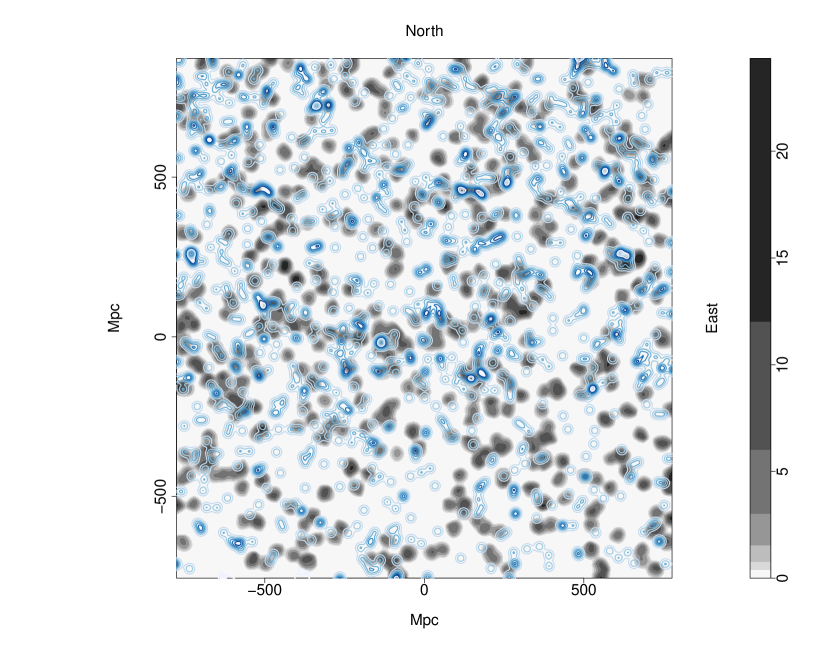
(a) Density distribution of the flat-fielded Mg II absorbers in the redshift slice $z=0.802\pm 0.060$ represented by the grey contours which have been smoothed using a Gaussian kernel of $\sigma=11$ Mpc and increase by a factor of two. Blue contours represent the DR16Q quasars with $i\leq 20.0$, in the same redshift slice as the Mg II absorbers, smoothed using a Gaussian kernel of $\sigma=11$ Mpc and increasing by a factor of two. The GA can be seen stretching across $\sim 1$ Gpc in the centre of the figure (at tangent-plane $y$-coordinate $\sim 0$ Mpc). Visually, the blue contours can be seen to follow the same general trajectory as the grey contours, indicating an association between the Mg II absorbers and the DR16Q quasars.

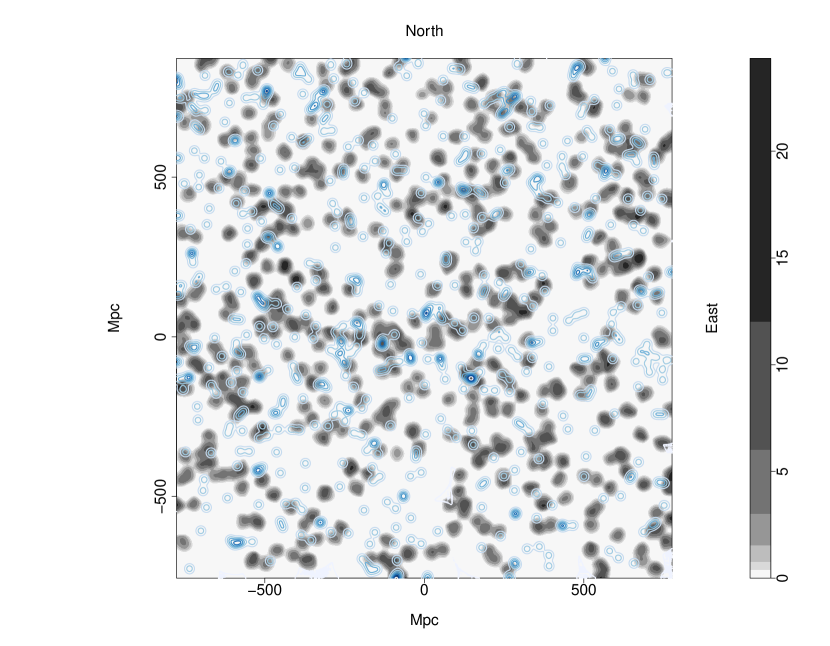
(b) Density distribution of the flat-fielded Mg II absorbers in the redshift slice $z=0.802\pm 0.060$ represented by the grey contours which have been smoothed using a Gaussian kernel of $\sigma=11$ Mpc and increase by a factor of two. Blue contours represent the DR16Q quasars, with $i\leq 19.5$, in the same redshift slice as the Mg II absorbers, smoothed using a Gaussian kernel of $\sigma=11$ Mpc and increasing by a factor of two. The GA can be seen stretching across $\sim 1$ Gpc in the centre of the figure (at tangent-plane $y$-coordinate $\sim 0$ Mpc). Visually, the blue contours can be seen to follow the same general trajectory as the grey contours, indicating an association between the Mg II absorbers and the DR16Q quasars.

Figure 14:

We continue with the DESI clusters, again selected for the same redshift interval as the GA — Fig. 15. Note that the redshifts for the DESI clusters are photometric, with redshift errors $\sim 0.024$ at $z\sim 0.9$ (Zou et al., 2021). (In contrast, we might expect the redshift errors for the quasars to be $\sim 0.003$.)

There is no compelling association of the DESI clusters and the GA, although there is perhaps a hint on the RHS. Possibly the substantial errors in the photometric redshifts are a factor in diluting any correspondence that might exist. An interesting feature in Fig. 15 is, however, the ‘cluster of clusters’ in the centre of the GA, largely coinciding with the central small gap in the Mg II absorbers of the GA. It could be a large supercluster, with the SZ cluster B18, mentioned previously, as one of its member clusters. We previously mentioned, in Section 2.2, that there appears to be a set of strong Mg II absorbers enveloping a circular hole in the centre of the GA. It seems likely that these enveloping strong absorbers and the central hole are related to this putative supercluster.

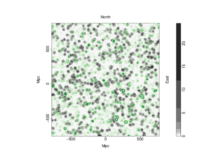
Figure 15: Density distribution of the flat-fielded Mg II absorbers in the redshift slice $z=0.802\pm 0.060$ represented by the grey contours which have been smoothed using a Gaussian kernel of $\sigma=11$ Mpc and increase by a factor of two. Green contours represent the DESI clusters, of all richnesses, in the same redshift slice as the Mg II absorbers, smoothed using a Gaussian kernel of $\sigma=11$ Mpc and increasing by a factor of two. The GA can be seen stretching across $\sim 1$ Gpc in the centre of the figure (at tangent-plane $y$-coordinate $\sim 0$ Mpc). There are no compelling connections between the DESI clusters and the Mg II absorbers.

The mean richness limit for the DESI clusters is $22.5$ (Zou et al., 2021). Fig. 16 shows the relationship between the Mg II absorbers and DESI clusters with richness $R\leq 22.5$. It suggests that there could be some association of the low-richness clusters with the Mg II absorbers, both for the GA and in general.

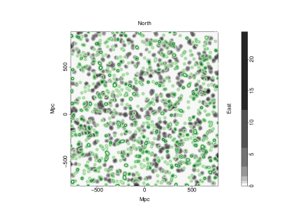
Figure 16: Density distribution of the flat-fielded Mg II absorbers in the redshift slice $z=0.802\pm 0.060$ represented by the grey contours which have been smoothed using a Gaussian kernel of $\sigma=11$ Mpc and increase by a factor of two. Green contours represent the DESI clusters, with the richness limit $R\leq 22.5$, in the same redshift slice as the Mg II absorbers, smoothed using a Gaussian kernel of $\sigma=11$ Mpc and increasing by a factor of two. The GA can be seen stretching across $\sim 1$ Gpc in the centre of the figure (at tangent-plane $y$-coordinate $\sim 0$ Mpc). There are a few occurrences of the green contours following the grey contours, indicating that there might be some association of low richness clusters with Mg II absorbers.

Finally, we compare the the DESI clusters with the DR16Q quasars — Fig. 17. As with the Mg II absorbers and DESI clusters, there appears to be no compelling association. However, again, the lowest-richness clusters suggest some association — Fig. 18.

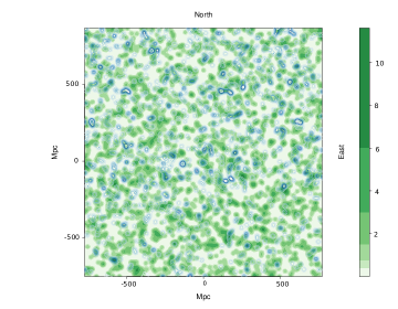
Figure 17: Density distribution of the DESI clusters in the redshift slice $z=0.802\pm 0.060$ represented by the green contours which have been smoothed using a Gaussian kernel of $\sigma=11$ Mpc and increase by a factor of two. Blue contours represent the DR16Q quasars, with the magnitude limit $i\leq 20.0$, in the same redshift slice as the DESI clusters, smoothed using a Gaussian kernel of $\sigma=11$ Mpc and increasing by a factor of two. There are no compelling connections between the DR16Q quasars and the DESI clusters.

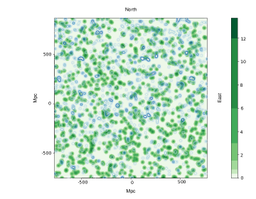
Figure 18: Density distribution of the DESI clusters in the redshift slice $z=0.802\pm 0.060$ represented by the green contours, increasing by a factor of two, which have been smoothed using a Gaussian kernel of $\sigma=11$ Mpc and limited to show only those clusters with a richness $R\leq 22.5$. Blue contours represent the DR16Q quasars, with the magnitude limit $i\leq 20$, in the same redshift slice as the DESI clusters, smoothed using a Gaussian kernel of $\sigma=11$ Mpc and increasing by a factor of two. There are a few occurrences of the blue contours following the green contours, indicating that there might be some association of DR16Q quasars with low richness clusters.

From the independent corroboration above, we suggest that the GA, and the Mg II absorbers in general, are associated with luminous quasars but not strongly with DESI clusters. However, there is potentially an association of the Mg II absorbers and the quasars with the low richness clusters. More statistical details of the relationship between Mg II absorbers, quasars and clusters will be investigated in our future work.

3 Discussions and Conclusions

In this paper we have presented the discovery of the Giant Arc (GA): a $\sim$ Gpc LSS at $z\sim 0.8$, mapped by Mg II absorption systems in the spectra of background quasars. The GA forms a large crescent shape on the sky that appears almost symmetrical. However, deeper analysis reveals some asymmetries in the GA, in the redshift and equivalent width (EW) distributions. The GA spans $\sim 1$ Gpc on the sky and has a redshift depth of $\sim 340$ Mpc (both proper sizes, present epoch) . Visually, we determine the GA as a single unit, but using a Minimal Spanning Tree (MST) type algorithm (see Section 2.3.1) it splits into two portions: a large portion (GA-main) and a small portion (GA-sub). We proposed in Section 2.3.1 that the two portions of the GA could in fact be connected in reality, since potentially one more background probe could lead to one more Mg II absorber that would connect the two portions. On its own, GA-main is a statistically-significant clustering of Mg II absorbers, with a membership of 44 Mg II absorbers, an MST-overdensity of $1.3\pm 0.3$, and a mass excess of $1.8\times 10^{18}M_{\odot}$. In these respects, the GA is comparable to the Huge-LQG (Clowes et al., 2013).

Three different statistical tests were applied to the GA to assess the significance of connectivity and clustering. The results of each are summarised here. (i) The SLHC / CHMS method calculates the significance of clustering between points of close proximity by comparing the volumes of the CHMS for each structure to the CHMS of structures in randomly distributed points in a cube. GA-main, containing 44 Mg II absorbers, has a significance of $(4.5\pm 0.6)\sigma$. GA-sub, containing 11 Mg II absorbers, has a significance of $(2.1\pm 0.9)\sigma$. Both GA-main and GA-sub have the same MST-overdensity of $\delta\rho/\rho=1.3\pm 0.3$. This fact could indicate, as we suspect, that both agglomerations are connected in reality. (ii) The CE test is a case-control $k$ nearest-neighbour algorithm that assesses the $p$-value of clustering in the field within an unevenly distributed population. A process of zooming into the GA field allows the GA to become increasingly dominant. In this way, we detect a $p$-value of $0.0027$ from the field seen in Fig. 9(a), equivalent to a significance of $3.0\sigma$. Applying this process of zooming to lower redshift fields at the same sky coordinates of the GA we do not detect any significant clustering. We then use our polygon approach that randomises points outside the GA while keeping the visually selected absorbers contained within the GA the same. The CE test detects similar $p$-value of clustering with the polygon approach, indicating that the GA is the true, dominating feature causing significant clustering. (iii) The PSA is a Fourier method of detecting clustering in the field on a physical scale. We apply the 2D PSA to the ‘zoomed’ GA field, Fig. 9(a), and find significant clustering at $\lambda_{c}\sim 270\,\mathrm{Mpc}$ with a significance of $4.8\sigma$. As with the CE test, we use our polygon approach and detect similar significant clustering scales. However, a small contribution from other absorbers in the field is also detected. We do expect this given the power of the PSA test, and it is clear that the GA is still the dominant contributor to the PSA result.

Clearly, the analysis of the GA is after the event of its discovery, as is unavoidable with unexpected discoveries in astrophysics and cosmology. We have applied several different approaches to mitigating any post-hoc aspects of analysing the statistical significance of the GA after discovery. We have performed techniques that aim to assess the GA unbiassedly, such as the polygon approach, varying redshift slices, zooming into the GA field, and randomised simulations. In the future we can apply the same techniques used for the GA field to the whole of the Mg II dataset. In addition, the Mg II dataset is quite complex, with features that need careful attention: for example, the inhomogeneities of the Mg II absorbers are superimposed on the inhomogeneities of the quasars (background probes) and of the survey. Finally, there are different Mg II databases available from different authors, each using different detection processes. We intend eventually to produce our own databases of Mg II detections that can be used consistently with past and future quasar-survey data releases.

The GA is now amongst several other very large LSS discoveries with sizes that exceed the theoretical upper-limit scale of homogeneity of (Yadav et al.2010). Potentially, there are other such significant structures in the rest of the Mg II database. We discuss that there are challenges in fairly characterising the population of structures due to the inhomogeneities in the background probes (quasars). However, the challenges can be managed with suitable care, allowing for the Mg II method of studying LSS to be fully exploited.

In Table LABEL:tab:lss_list, we listed some of the very large LSSs, and also some of the reported CMB anomalies. In standard cosmology we expect to find evidence for a homogeneous and isotropic universe. However, the accumulated set of LSS and CMB anomalies now seems sufficient to constitute a prima facie challenge to the assumption of the Cosmological Principle (CP). A single anomaly, such as the GA on its own, could be expected in the standard cosmological model. For example, Marinello et al. (2016) find that the Huge-LQG (Clowes et al., 2013), a structure comparable in size to the GA, is, by itself (there are others), compatible with the standard cosmological model. However, Marinello et al. (2016) state that this is on the condition that only one structure as large as the Huge-LQG is found in a field $\sim 5$ times the sample survey, in this case, the DR7QSO quasar database for $1.2\leq z\leq 1.6$. Note that the GA is found in the combined footprint from DR7QSO and DR12Q (the combined footprint being almost the same area as the individual footprints), in a narrow redshift interval, so its challenge to the CP seems likely to be exacerbated. Of course, the GA is now the fourth largest LSS, so there are, at minimum, four LSSs comparable to the size of the Huge-LQG, plus several other LSSs exceeding the scale of homogeneity. We suggest that there is a need to explore other avenues within cosmology that could explain multiple, very large LSSs.

We bring attention to the Sloan Great Wall (SGW) (Gott et al., 2005), which is a large, wall-like filament in the relatively local universe. The SGW is $\sim 450$ Mpc in its longest dimension, which is $\sim 0.5$ times the length of the GA. One can note some of the similarities between the SGW and the GA, such as the general shape and comoving size — they are both long, filamentary and curved walls made up of galaxies and galaxy clusters —, and so perhaps also envision a LSS such as the GA as a precursor to the SGW. The GA is at a redshift of $\sim 0.8$ which means we are seeing it when the universe was only half its present age. Perhaps the SGW, at an earlier epoch, initially looked more like the GA. At this point, these ideas are speculative only, but experimenting with simulations (possibly even with alternative cosmological models) could conceivably elucidate such hypothetical connections between structures like the GA and the SGW.

Data availability statement

The datasets were derived from sources in the public domain: https://www.guangtunbenzhu.com/jhu-sdss-metal-absorber-catalog.

References

- Bagchi et al. (2017) Bagchi J., Sankhyayan S., Sarkar P., Raychaudhury S., Jacob J., Dabhade P., 2017, ApJ, 844:25
- Balázs et al. (2015) Balázs L.G., Bagoly Z., Hakkila J.E., Horváth I., Kóbori J., Rácz I.I., Tóth L.V., 2015, MNRAS, 452, 2236
- Bordoloi et al. (2011) Bordoloi R., Lilly S.J., Kacprzak G.G., Churchill C.W., 2011, ApJ, 784, 108
- Burenin et al. (2018) Burenin R.A. et al., 2018, Astron. Letters, 44, 297
- Chen et al. (2010) Chen H.-W., Wild V., Tinker J.L., Gauthier J.-R., Helsby J.E., Shectman S.A., Thompson I.B., 2010, ApJL, 724, L176
- Christian (2020) Christian S., 2020, MNRAS, 495, 4291
- Churchill et al. (2005) Churchill C.W., Kacprzak G.G., Steidel C.C., 2005, Proc. IAU Colloq., 199
- Churchill et al. (2000) Churchill C.W. et al., 2000, ApJ, 130, 91
- Clowes (1986) Clowes R.G., 1986, MNRAS, 218, 139
- Clowes & Campusano (1991) Clowes R.G., Campusano L.E., 1991, MNRAS, 249, 218
- Clowes et al. (2012) Clowes R.G., Campusano L.E., Graham M.J., Söchting I.K., 2012, MNRAS, 419, 556
- Clowes et al. (2013) Clowes R.G., Harris K.A., Raghunathan S., Campusano L.E., Söchting I.K., Graham M.J., 2013, MNRAS, 429, 2910
- Colin et al. (2019) Colin J., Mohayaee R., Rameez M., Sarkar S., 2019, A&A, 631, L13
- Cuzick & Edwards (1990) Cuzick J., Edwards R., 1990, J. R. Statist. Soc. B, 52, 73
- Dutta et al. (2017) Dutta R., Srianand R., Gupta N., Joshi R., 2017, MNRAS, 468, 1029
- Evans et al. (2013) Evans J.L., Churchill C.W., Murphy M.T., Nielsen N.M., Klimek E.S., 2013, ApJ, 768
- French (2020) French J., 2020, https://cran.r-project.org/web/packages/smacpod
- (18) Friday T., Clowes R.G., Williger G.M., 2022, MNRAS, 511, 4159
- Geller & Huchra (1989) Geller M.J., Huchra J.P., 1989, Sci, 246, 897
- Gott et al. (2005) Gott J.R., III, Jurić M., Schlegel D., Hoyle F., Vogeley M., Tegmark M., Bahcall N., Brinkmann J., 2005, ApJ, 624, 463
- Hinrichsen et al. (2009) Hinrichsen V.L., Klassen A.C., Song C., Kulldorff M., 2009, Int. J. Health Geogr., 8:41
- (22) Horváth I., Hakkila J., Bagoly Z., 2014, A&A, 561, L12
- Horvath et al. (2020) Horvath I., Szécsi D., Hakkila J., Szabó Á., Racz I.I., Tóth L.V., Pinter S., Bagoly Z., 2020, MNRAS, 498, 2544
- Hutsemékers (1998) Hutsemékers D., 1998, A&A, 332, 410
- Hutsemékers & Lamy (2001) Hutsemékers D., Lamy H., 2001, A&A, 367, 381
- Hutsemékers et al. (2005) Hutsemékers D., Cabanac R., Lamy H., Sluse D., 2005, A&A, 441, 915
- Hutsemékers et al. (2014) Hutsemékers D., Braibant L., Pelgrims V., Sluse D., 2014, A&A, 572, A18
- Kacprzak et al. (2008) Kacprzak G.G., Churchill C.W., Steidel C.C., Murphy M.T., 2008, ApJ, 135, 922
- (29) Keenan R.C., Barger A.J., Cowie L.L., 2013, ApJ, 775:62
- Lanzetta & Bowen (1990) Lanzetta K.M., Bowen D., 1990, ApJ, 357, 321
- (31) Lee J.C., Hwang H.S., Song H., 2021, MNRAS, 503, 4309
- Lietzen et al. (2016) Lietzen H. et al., 2016, A&A, 588, L4
- Lopez (2019) Lopez A.M., 2019, MSc thesis, Univ. of Central Lancashire
- Lyke et al. (2020) Lyke B.W. et al., 2020, ApJS, 250:8
- Marchã & Browne (2021) Marchã M.J.M., Browne I.W.A., 2021, MNRAS, 507, 1361
- Marinello et al. (2016) Marinello G.E., Clowes R.G., Campusano L.E., Williger G.M., Söchting I.K., Graham M.J., 2016, MNRAS, 461, 2267
- Meliker et al. (2009) Meliker J.R., Jacquez G.M., Goovaerts P., Copeland G., Yassine M., 2009, Cancer Causes Control, 20, 1061
- Migkas et al. (2020) Migkas K., Schellenberger G., Reiprich T.H., Pacaud F., Ramos-Ceja M.E., Lovisari L., 2020, A&A, 636, A15
- Nadathur (2013) Nadathur S., 2013, MNRAS, 434, 398
- Pâris et al. (2017) Pâris I. et al., 2017, A&A, 597, A79
- Pilipenko (2007) Pilipenko S. V., 2007, Astron. Rep., 51, 820:829
- Pomarède et al. (2020) Pomarède D., Tully R.B., Graziani R., Courtois H.M., Hoffman Y., Lezmy J., 2020, ApJ, 897:133
- Schneider et al. (2010) Schneider D.P. et al., 2010, AJ, 139, 2360
- Schwarz et al. (2016) Schwarz D.J., Copi C.J., Huterer D., Starkman G.D., 2016, Class. Quantum Grav., 33, 184001
- Secrest et al. (2021) Secrest N.J., von Hausegger S., Rameez M., Mohayaee R., Sarkar S., Colin J., 2021, ApJL, 908:L51
- Song & Kulldorff (2003) Song C., Kulldorff M., Int. J. Health Geogr., 2003, 2:9
- Steidel (1995) Steidel C. C., 1995, in G. Meylan ed., ESO Workshop on Quasar Absorption Lines, Springer-Verlag, 139
- Steidel et al. (2002) Steidel C.C. et al., 2002, ApJ, 570, 526
- (49) Thomas S.A., Abdalla F.B., Lahav O., 2011, PRL, 106, 241301
- Webster (1976a) Webster A.S., 1976a, MNRAS, 175, 61
- Webster (1976b) Webster A.S., 1976b, MNRAS, 175, 71
- Webster (1982) Webster A.S., 1982, MNRAS, 199, 683
- Whitbourn & Shanks (2016) Whitbourn J.R., Shanks T., 2016, MNRAS, 459, 496
- Williger et al. (2002) Williger G.M., Campusano L.E., Clowes R.G., Graham M.J., 2002, ApJ, 578, 708
- (55) Yadav J.K., Bagla J.S., Khandai N., 2010, MNRAS, 405, 2009
- Zhu & Ménard (2013) Zhu G., Ménard B., 2013, ApJ, 770:130
- Zou et al. (2021) Zou H. et al., 2021, ApJS, 253:56