January 2022

Target space entanglement in a matrix model for the bubbling geometry

Asato Tsuchiya and Kazushi Yamashiro

Department of Physics, Shizuoka University
836 Ohya, Suruga-ku, Shizuoka 422-8529, Japan
Graduate School of Science and Technology, Shizuoka University
836 Ohya, Suruga-ku, Shizuoka 422-8529, Japan

We study the target space entanglement entropy in a complex matrix model that describes the chiral primary sector in $\mathcal{N}=4$ super Yang-Mills theory, which is associated with the bubbling AdS geometry. The target space for the matrix model is a two-dimensional plane where the eigenvalues of the complex matrix distribute. The eigenvalues are viewed as the position coordinates of fermions, and the eigenvalue distribution corresponds to a droplet formed by the fermions. The droplet is identified with one that specifies a boundary condition in the bubbling geometry. We consider states in the matrix model that correspond to $AdS_{5}\times S^{5}$, an AdS giant graviton and a giant graviton in the bubbling geometry. We calculate the target space entanglement entropy of a subregion for each of the states in the matrix model as well as the area of the boundary of the subregion in the bubbling geometry, and find a qualitative agreement between them.

1 Introduction

It has been recognized that quantum entanglement plays a crucial role in constructing a quantum theory of gravity. As seen typically in the Ryu-Takayanagi formula[1], quantum entanglement has information on geometry of space-time. The formula tells that when the space where a field theory is defined is divided into a subregion and its complement, the entanglement entropy of the subregion is proportional to the area of minimal surface in the bulk whose boundary agrees with that of the subregion. The entanglement entropy in the formula is here called the base space entanglement entropy.

Recently, a new type of quantum entanglement entropy in field theories which is called the target space entanglement entropy has been investigated in the context of the gauge/gravity correspondence[2, 5, 3, 4, 6, 7]. It is defined by dividing the configuration space of fields into a subregion and its complement. In particular, the target space entanglement entropy can be defined in $(0+1)$-dimensional field theory, namely quantum mechanics, although the base space entanglement entropy cannot be defined there. For instance, in matrix quantum mechanics, the target space is identified with a space where the eigenvalues of the matrix distribute. It is nontrivial to define entanglement entropy in gravitational theories because of division of dynamical spaces. It has been conjectured in [3] that in the gauge/gravity correspondence, the entanglement entropy in the bulk on the gravity side can be defined by the target space entanglement entropy on the gauge theory side. In particular, the target space entanglement entropy of a subregion in the D0-brane quantum mechanics[8] is expected to be proportional with factor of proportionality $1/4G_{N}$ to the area of boundary of the corresponding subregion in the bulk on the gravity side.

In this paper, we study this issue in the D3-brane holography, namely a conjectured correspondence between $\mathcal{N}=4$ super Yang-Mills theory (SYM) and type IIB superstring theory on $AdS_{5}\times S^{5}$[9, 10, 11]. Here we focus on a correspondence between the chiral primary sector and the bubbling AdS geometry[12, 13, 14]. The chiral primary sector can be described by a complex matrix model[15] whose target space is a two-dimensional plane where the eigenvalues of the complex matrix distribute (see also [16]). The eigenvalues can be viewed as the position coordinates of fermions in the harmonic oscillator potential in the two-dimensional plane, and the eigenvalue distribution corresponds to a droplet formed by the fermions. The target space can be identified with a two-dimensional plane in the bubbling geometry where a boundary condition for a function that determines a half-BPS solution with $R\times SO(4)\times SO(4)$ symmetry in type IIB supergravity is specified by giving a droplet. We calculate the target space entanglement entropy of a subregion in the two-dimensional plane for each of states that are specified by droplets corresponding to $AdS\times S^{5}$, an AdS giant graviton and a giant graviton as well as the area (length) of boundary of the corresponding subregion in the bubbling geometry. We find a qualitative agreement between the target space entanglement entropy and the area.

This paper is organized as follows. In section 2, we review some materials that we will need in this paper: a complex matrix model that describes the chiral primary sector in $\mathcal{N}=4$ SYM on $R\times S^{3}$, the bubbling AdS geometry, and the target space entanglement entropy. In section 3, we calculate the entanglement entropy in the complex matrix model. In section 4, we calculate the area of boundary in the bubbling geometry and compare it with the target space entanglement entropy. Section 5 is devoted to conclusion and discussion. In appendices, some details are gathered.

2 Review

2.1 Complex matrix model and fermions in two-dimensional plane

In this subsection, we review a complex matrix model that describes the chiral primary sector of $\mathcal{N}=4$ SYM on $R\times S^{3}$. The chiral primary operators take the form

$$\mathcal{O}^{J_{1},J_{2},\cdots,J_{K}}(t)=\prod^{K}_{a=1}\mbox{Tr}(Z^{J_{a}})\ ,$$ (2.1)

where $Z=\frac{1}{\sqrt{2}}(\phi_{1}+i\phi_{2})$ with $\phi_{1}$ and $\phi_{2}$ being two of six scalars in $\mathcal{N}=4$ SYM. These operators are half-BPS holomorphic operators. Kaluza-Klein gravitons, AdS giant gravitons and giant gravitons on the gravity side are represented in terms of a linear combination of the operators (2.1). It was shown in [15] that the dynamics of the operators is described by a complex matrix model which is obtained by dimensionally reducing the free part of the action for $Z$ on $R\times S^{3}$ to $R$. The complex matrix model is a matrix quantum mechanics defined by

$$\mathcal{Z} =\int[dZ(t)dZ^{\dagger}(t)]e^{iS}\ ,$$

$$S =\int dt\mbox{Tr}(\dot{Z}(t)\dot{Z^{\dagger}}(t)-Z(t)Z^{\dagger}(t))=\int dt\sum_{i,j}(\dot{Z}(t)_{ij}\dot{Z^{*}}(t)_{ij}-Z(t)_{ij}Z^{*}(t)_{ij})\ ,$$ (2.2)

where $Z(t)$ is an $N\times N$ complex matrix depending on the time, and the path integral measure is defined by a norm in matrix configuration space,

$$||dZ(t)||^{2}=2\mbox{Tr}(dZ(t)dZ^{\dagger}(t))=2\sum_{i,j}dZ(t)_{ij}dZ^{*}(t)_{ij}\ .$$ (2.3)

The potential term in the action comes from the coupling of the conformal matter to the curvature of $S^{3}$. We have rescaled the field and the time appropriately.

The hamiltonian is given by

$$\hat{H}=\sum_{i,j}\left(-\frac{\partial}{\partial Z_{ij}\partial Z^{*}_{ij}}+Z_{ij}Z^{*}_{ij}\right)\ .$$ (2.4)

The normalized wave function of the ground state is given by

$$\chi_{0}=\frac{1}{\pi^{\frac{N^{2}}{2}}}e^{-\mbox{Tr}(ZZ^{\dagger})}=\frac{1}{\pi^{\frac{N^{2}}{2}}}e^{\Sigma_{i,j}Z_{ij}Z^{*}_{ij}}\ ,$$ (2.5)

and the wave functions of excited states that correspond to the chiral primary states are given by

$$\chi^{(J_{1},\cdots,J_{K})}=\left(\prod^{K}_{a=1}\mbox{Tr}(Z^{J_{a}})\right)\chi_{0}\ .$$ (2.6)

The energy eigenvalues of these states are $N^{2}+\Sigma^{K}_{a=1}J_{a}$.

The complex matrix $Z$ is decomposed as $Z=UTU^{\dagger}$ in terms of a unitary matrix $U$ and an upper triangular matrix $T$. The eigenvalues of $Z$ are given by $z_{i}=T_{ii}\;(i=1,\cdots,N)$. The wave functions (2.6) are rewritten in terms of $z_{i}$ and $T_{ij}\;(i<j)$ as

$$\chi^{(J_{1},\cdots,J_{K})} =\left(\prod^{K}_{a=1}\sum_{i_{a}}z^{J_{a}}_{i_{a}}\right)\chi_{0}\ ,$$

$$\chi_{0} =\frac{1}{\pi^{\frac{N^{2}}{2}}}e^{-\Sigma_{i}z_{i}z^{*}_{i}-\Sigma_{j<k}T_{jk}T^{*}_{jk}}\ ,$$ (2.7)

while the path integral measure as

$$\int\prod_{i,j}dZ_{ij}dZ^{*}_{ij}=\int\prod_{i>j}dH_{ij}dH^{*}_{ij}\prod_{k<l}dT_{kl}dT^{*}_{kl}\prod_{m}dz_{m}dz^{*}_{m}|\Delta(z)|^{2}\ ,$$ (2.8)

where $\Delta(z)=\prod_{i<j}(z_{i}-z_{j})$ and $dH=-iU^{\dagger}dU$. We can absorb $\Delta(z)$ into the wave function and define a new wave function $\chi_{F}$ by $\chi_{F}\equiv\Delta(z)\chi$. Then, $\chi_{F}$ is represented as a certain linear combination of

$$\frac{1}{\sqrt{N!}}\det(\Phi_{l_{i}}(z_{j},z^{*}_{j}))\times\prod_{j<k}\Phi_{0}(T_{jk},T^{*}_{jk})\ ,$$

$$\mbox{with}\;\;\sum_{i}l_{i}=\frac{N(N-1)}{2}+\sum_{a=1}^{K}J_{a}\ ,$$ (2.9)

where $\Phi_{l}(z,z^{*})$ are the wave function of the lowest Landau level which takes the form

$$\Phi_{l}(z,z^{*})=\sqrt{\frac{2^{l}}{l!\pi}}z^{l}e^{-zz^{*}}\ .$$ (2.10)

As reviewed in appendix A, the wave function $\Phi(z,z^{*})$ can be viewed as a wave function of the holomorphic sector for a particle in the harmonic oscillator potential in two-dimensional plane. (2.9) is a wave function for $N$ fermions and $\frac{1}{2}N(N-1)$ bosons in the harmonic oscillator potential. The eigenvalues $z_{i}$ of $Z$ can be viewed as the coordinates of $N$ fermions and the total energy of these fermions is $\frac{1}{2}N(N+1)+\Sigma^{K}_{a=1}J_{a}$, where $\frac{1}{2}N(N+1)$ is the energy of the ground state of the fermions. On the other hand, the bosons whose coordinates are $(T_{ij},T_{ij}^{*})$ are always in the ground state. Hence, we can integrate out $T_{ij}$ and concentrate on $\frac{1}{\sqrt{N!}}\det(\Phi_{l_{i}}(z_{j},z^{*}_{j}))$ in (2.9). In this way, the holomorphic sector of the complex matrix model, which describes the dynamics of the operators (2.1), reduces to a system of $N$ fermions in the two-dimensional harmonic oscillator potential. For large $N$, we can view the eigenvalue distribution corresponding to a state as a droplet in the complex plane, which is formed by $N$ fermions.

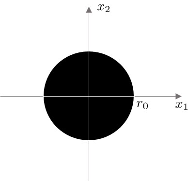
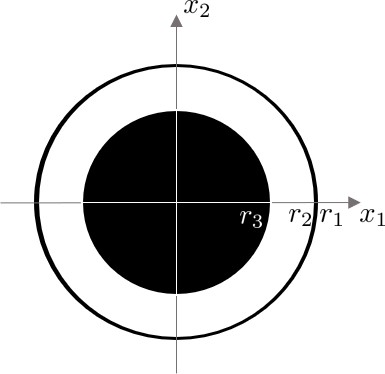
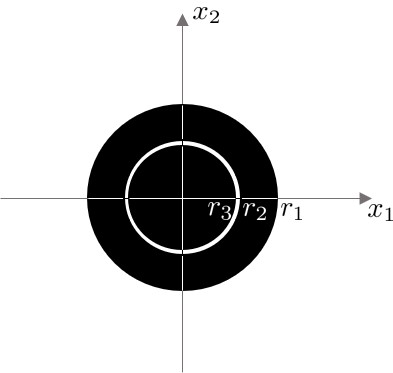
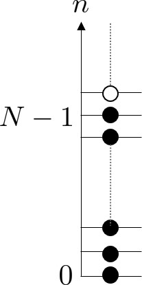
(a) $AdS_{5}\times S^{5}$	(b) AdS giant graviton	(c) giant graviton
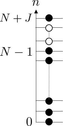
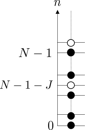
(d) $AdS_{5}\times S^{5}$	(e) AdS giant graviton	(f) giant graviton

Figure 1: (1), (1) and (1) are droplets of the states that correspond to $AdS_{5}\times S^{5}$, an AdS giant graviton and a giant graviton, respectively. (1), (1) and (1) are the occupied energy levels of the states that correspond to $AdS_{5}\times S^{5}$, an AdS giant graviton and a giant graviton, respectively.

In what follows, we consider three particular states whose wave functions are given by

$$\frac{1}{\sqrt{N!}}\det(\Phi_{l_{i}}(z_{j},z^{*}_{j}))$$ (2.11)

in (2.9). The first one is the ground state where $l_{1}=0,\ l_{2}=1,\ \cdots,\ l_{N}=N-1$. We show the corresponding droplet in Fig. 1 and the occupied energy levels in Fig. 1. This corresponds to $AdS_{5}\times S^{5}$ in the bubbling geometry. The second one is an excited state where $l_{1}=0,\ l_{2}=1,\ \cdots,\ l_{N}=N-1,\ l_{N+1}=N+J$. Note that the total number of fermions is $N+1$. We show the corresponding droplet in Fig. 1 and the occupied energy levels in Fig. 1. This corresponds to a bubbling geometry where there exists an AdS giant graviton, which is a D3-brane wrapped on $S^{3}$ in $AdS_{5}$. The third one is an excited state where $l_{1}=0,\ l_{2}=1,\ \cdots,\ l_{N-1-J}=N-2-J,\ l_{N-J}=N-J,\ \cdots,\ l_{N-1}=N-1$. Note that the total number of fermions is $N-1$. We show the corresponding droplet in Fig .1 and the occupied energy levels in Fig. 1. This corresponds to a bubbling geometry where there exists a giant graviton, which is a D3-brane wrapped on $S^{3}$ in $S^{5}$. The wave function $\Phi_{l}(z,z^{*})$ is localized on a circle centered at the origin with the radius $\sqrt{l}$. Hence, $r_{0}$ in Fig. 1 is equal to $\sqrt{N}$ for large $N$.

2.2 Bubbling geometry

In this subsection, we review the bubbling geometry developed by Lin, Lunin and Maldacena. They gave the general form of half-BPS solutions with $R\times SO(4)\times SO(4)$ symmetry in type IIB supergravity [14]. The metric takes the form

$$ds^{2}=-h^{-2}\left[dt+\sum_{i=1}^{2}V_{i}dx^{i}\right]^{2}+h^{2}\left[dy^{2}+\sum_{i=1}^{2}dx^{i}dx^{i}\right]+ye^{G}d\Omega_{3}^{2}+ye^{-G}d\tilde{\Omega}^{2}_{3}\ ,$$ (2.12)

where

$$h^{-2}=2y\cosh G,\ \ z=\frac{1}{2}\tanh G,\ \ y\partial_{y}V_{i}=\epsilon_{ij}\partial_{j}z,\ \ y(\partial_{i}V_{j}-\partial_{j}V_{i})=\epsilon_{ij}\partial_{y}z\ .$$ (2.13)

The function $z(x_{1},x_{2},y)$ completely determines the solutions and obeys a differential equation

$$\partial_{i}\partial_{i}z+y\partial_{y}\left(\frac{\partial_{y}z}{y}\right)=0\ .$$ (2.14)

The function $z$ is fixed by specifying a boundary condition at $y=0$. It turns out that $z$ must take $1/2$ or $-1/2$ at $y=0$. It is convenient to assign ‘black’ to the region with $z=-1/2$ and ‘white’ to the region with $z=1/2$. In this way, there is a correspondence between divisions of the $x_{1}-x_{2}$ plane into black and white regions and half-BPS solutions with $R\times SO(4)\times SO(4)$ symmetry. One can identify a two-dimensional plane specified by $y=0$ in the bubbling geometry with the target space in the complex matrix model such that black regions correspond to droplets in the target space. Figs 1, 1 and 1 correspond to $AdS_{5}\times S^{5}$, an AdS giant graviton and a giant graviton, respectively, as mentioned before. Here $r_{0}$ in Fig.1 is related to the radius of $AdS_{5}$ as $r_{0}=R_{AdS}^{2}=\sqrt{N}$.

2.3 Target Space Entanglement Entropy

In this subsection, we briefly review the target space entanglement entropy[2]. For concreteness, we consider a quantum mechanics of $N$ identical particles in $d$ dimensions. In this case, the target space is the $d$-dimensional space where $N$ particle reside. We divide the target space into a subregion $A$ and its complement $\bar{A}$. Then, the total Hilbert space $\mathcal{H}$ is decomposed as

$$\mathcal{H}=\bigoplus_{n}\mathcal{H}_{A,n}\otimes\mathcal{H}_{\bar{A},n}\ ,$$ (2.15)

where $n$ labels a sector where $n$ particles exist in $A$ and $N-n$ particles exist in $\bar{A}$. The target space entanglement entropy of the subregion $A$ is given by

$$S_{A}=-\sum_{n}p_{n}\log p_{n}+\sum_{n}p_{n}S_{A,n}\ .$$ (2.16)

The first and second terms in the RHS is classical and quantum parts, respectively. Here $p_{n}$ is the probability of realization of the sector $n$, which is given by

$$p_{n} =\begin{pmatrix}N\\ n\\ \end{pmatrix}\int_{A}\prod_{a=1}^{n}d^{d}x_{a}\int_{\bar{A}}\prod_{b=n+1}^{N}d^{d}y_{b}|\psi(\vec{x}_{1},\cdots,\vec{x}_{n},\vec{y}_{n+1},\cdots,\vec{y}_{N})|^{2}\ .$$ (2.17)

$S_{A,n}$ is interpreted as the entanglement entropy of the subregion $A$ in the sector $n$, which is given by

$$S_{A,n}=-\mbox{tr}_{A,n}\rho_{A,n}\log\rho_{A,n}\ ,$$ (2.18)

where $\rho_{A,n}$ is the reduced density matrix of the sector $n$ and its matrix elements in the coordinate basis are given by

$$\bra{\vec{x}}\rho_{A,n}\ket{\vec{x}^{\prime}}=\frac{1}{p_{n}}\begin{pmatrix}N\\ n\\ \end{pmatrix}\int_{\bar{A}}\prod_{b=n+1}^{N}d^{d}y_{b}\psi(\vec{x},\vec{y})\psi^{*}(\vec{x^{\prime}},\vec{y})\ .$$ (2.19)

As a particular example[6], we consider $N$ identical fermions which are not interacting each other and the wave function of which is given by a Slater determinant

$$\psi(\vec{x}_{1},\cdots\vec{x}_{N})=\frac{1}{\sqrt{N!}}\det(\chi_{i}(\vec{x}_{j}))\ ,$$ (2.20)

where $\chi_{i}(\vec{x})$ are orthonormal single-body wave functions:

$$\int d^{d}x\chi_{i}^{*}(\vec{x})\chi_{j}(\vec{x})=\delta_{ij}\ .$$ (2.21)

We introduce an $N\times N$ overlap matrix $X_{ij}$

$$X_{ij}\equiv\int_{A}d^{d}x\ \chi_{i}(\vec{x})\chi^{*}_{j}(\vec{x})\ ,$$ (2.22)

$X_{ij}$ is a hermitian matrix so that it is diagonalized by a unitary matrix $U_{ij}$. The eigenvalues of $X_{ij}$ denoted by $\lambda_{i}$ are given by

$$\lambda_{i}=\int_{A}|\tilde{\chi}_{i}(\vec{x})^{2}|\ ,$$ (2.23)

where $\tilde{\chi}_{i}(\vec{x})=U_{ij}\chi_{j}(\vec{x})$. $\lambda_{i}$ is the probability of existence in the region $A$ when the wave function for a particle is given by $\tilde{\chi}_{i}(\vec{x})$.

$p_{n}$ in (2.17) is given by

$$p_{n}=\sum_{I\in F_{n}}\prod_{i\in I}\lambda_{i}\prod_{j\in\bar{I}}(1-\lambda_{j})\ .$$ (2.24)

Here $F_{n}$ is a set of all subsets of $\{1,\ldots,N\}$ that consist of $n$ elements. We see that $p_{n}$ is indeed the probability that $n$ particles exist in the region $A$ when the probability that each of $N$ particles exists in $A$ is given by $\lambda_{i}$.

The matrix elements of $\rho_{A,n}$ in (2.19) are

$$\bra{\vec{x}}\rho_{A,n}\ket{\vec{x}^{\prime}}=\frac{1}{p_{n}}\sum_{I\in F_{n}}\lambda_{I}\bar{\lambda}_{I}\psi_{I}(\vec{x})\psi_{I}^{*}(\vec{x^{\prime}})\ ,$$ (2.25)

where we put $\lambda_{I}\equiv\prod_{i\in I}\lambda_{i},\;\;\bar{\lambda}_{I}\equiv\prod_{i\in I}(1-\lambda_{i})$ for an element $I$ of $F_{n}$ and introduce a wave function for $n$ particles

$$\psi_{I}=\frac{1}{\sqrt{\lambda_{I}}}\sum_{\sigma\in S_{n}}\frac{(-1)^{\sigma}}{\sqrt{n!}}\tilde{\chi}_{n_{\sigma(1)}}(\vec{x}_{1})\cdots\tilde{\chi}_{n_{\sigma(n)}}(\vec{x}_{n})\ .$$ (2.26)

The quantum part is calculated as

$$\sum^{N}_{n=0}p_{n}S_{A,n}=\sum^{N}_{n=0}p_{n}\log p_{n}-\sum^{N}_{n=0}\sum_{I\in F_{n}}\lambda_{I}\bar{\lambda}_{I}\log(\lambda_{I}\bar{\lambda}_{I})\ .$$ (2.27)

Thus, we see from (2.25) and (2.27) that the total target space entanglement entropy (2.16) is given by

$$S_{A}=-\sum^{N}_{n=0}\sum_{I\in F_{n}}\lambda_{I}\bar{\lambda}_{I}\log(\lambda_{I}\bar{\lambda}_{I}).$$ (2.28)

By introducing $H(\lambda)\equiv-\lambda\log\lambda-(1-\lambda)\log(1-\lambda)$, we represent (2.28) as

$$S_{A}=\sum_{i=1}^{N}H(\lambda_{i})\ .$$ (2.29)

Here $H(\lambda)$ is the Shannon entropy for the Bernoulli distribution $(\lambda,1-\lambda)$.

3 Target Space Entanglement Entropy in the complex matrix model

In this section, we calculate the target space entanglement entropy for the three states in the complex matrix model introduced in section 2.1. We consider a circle centered at the origin with the radius $r$ as a subregion $A$. Then, the overlap matrix (2.22) is given by

$$X_{ll^{\prime}}(A) =2\int_{A}dzdz^{*}\Phi_{l}(z,z^{*})\Phi_{l^{\prime}}(z,z^{*})$$

$$=\delta_{ll^{\prime}}a_{l}(r)\ .$$ (3.1)

Note that this matrix is diagonal and its eigenvalues $\lambda_{l}$ are

$$\lambda_{l}=a_{l}(r)=\frac{\gamma[l+1,r^{2}]}{\Gamma[l+1]}\ .$$ (3.2)

$\lambda_{l}$ is the provability of existence in $A$ of a single particle. Here $\Gamma[x]$ is the gamma function and $\gamma[a,x]$ is the incomplete gamma function:

$$\gamma[a,x]=\int_{0}^{x}t^{a-1}e^{-t}dt\ .$$ (3.3)

By using (2.28), we obtain the target space entanglement entropy of the subregion $A$:

$$S(r,N)=\sum^{N}_{i=1}H(a_{l_{(i)}}(r)),\ \ \ H(a_{l_{(i)}}(r))=-a_{l_{(i)}}(r)\log a_{l_{(i)}}(r)-(1-a_{l_{(i)}}(r))\log(1-a_{l_{(i)}}(r))\ .$$ (3.4)

First, let us consider the target space entanglement entropy for the ground state indicated in Figs. 1 and 1, which correspond to $AdS_{5}\times S^{5}$ in the bubbling geometry. In this case, the single-body states with $l=0,\cdots,N-1$ are occupied. Thus, (3.4) is

$$S_{0}(r,N)=\sum^{N-1}_{l=0}H(a_{l}(r)),\ H(a_{l}(r))=-a_{l}(r)\log a_{l}(r)-(1-a_{l}(r))\log(1-a_{l}(r))\ .$$ (3.5)

In Fig. 2, we plot the target space entanglement entropy $S_{0}$ for $N=40,\ 60,\ 80,\ 100$ against $r$. We see that $S_{0}$ is proportional to $r$ as $S_{0}=1.81r$ when the subregion $A$ is included in the droplet, namely $r<\sqrt{N}$. This behavior shows that the entanglement entropy is proportional to the area of boundary of the subregion $A$. The fact that $S_{0}=0$ when the droplet is included in the subregion $A$, namely $r>\sqrt{N}$, shows that there is no entanglement between inside and outside of $A$ because all particles are confined in $A$. This is a finite $N$ effect .

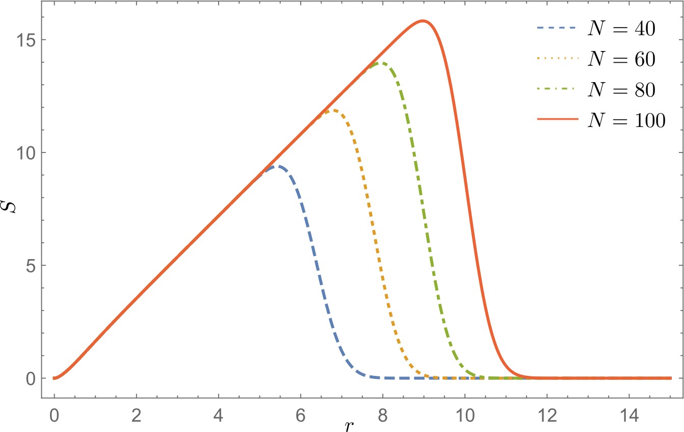
Figure 2: The target space entanglement entropy for the ground state $S_{0}$ with $N=40,\ 60,\ 80,\ 100$ are plotted against the radius $r$ of the subregion $A$.

Second, we calculate the target space entanglement entropy for an excited state corresponding to an AdS giant graviton indicated in Figs. 1 and 1. (3.4) in this case is

$$S_{AdS}(r,N,J)=\sum^{N-1}_{i=0}H(a_{i}(r))+H(a_{N+J}(r))\ .$$ (3.6)

In Fig. 3, we plot $S_{AdS}$ for $N=50$ and $J=50$ against $r$. In order to see only the contribution of the AdS giant graviton to the target space entanglement entropy, we subtract $S_{0}$ from $S_{AdS}$. In Fig. 4, we plot $S_{AdS}^{\prime}=S_{AdS}(r,50,50)-S_{0}(r,50)$ against $r$. Note here that $N$ for $S_{AdS}$ is different from that for $S_{0}$. We see that there is a peak at $r=\sqrt{N+1+J}$, which is considered as the position of the AdS giant graviton.

Third, (3.4) for the excited state corresponding to a giant graviton indicated in Figs. 1 and 1 is

$$S_{g}(r,N,J)=\sum^{N-2-J}_{i=0}H(a_{i}(r))+\sum^{N}_{j=N-J}H(a_{j}(r))\ .$$ (3.7)

In Fig. 5, we plot $S_{g}$ for $N=100$ and $J=49$ and $S_{0}$ for $N=100$ against $r$. In order to see only the contribution of the giant graviton to the target space entanglement entropy, we plot $S_{g}^{\prime}=S_{g}(r,100,49)-S_{0}(r,100)$ against $r$ in Fig. 6. We see that there is a peak at $r=\sqrt{N-J}$, which is considered as the position of the giant graviton.

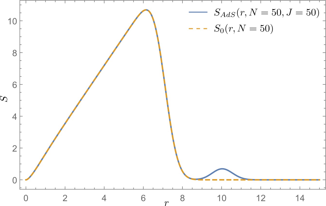
Figure 3: The solid line represents the target space entanglement entropy for the state corresponding to the AdS giant graviton $S_{AdS}(r)$ with $N=50$ and $J=50$, while the dashed line represents the target space entanglement entropy for the ground state $S_{0}(r)$ with $N=50$.

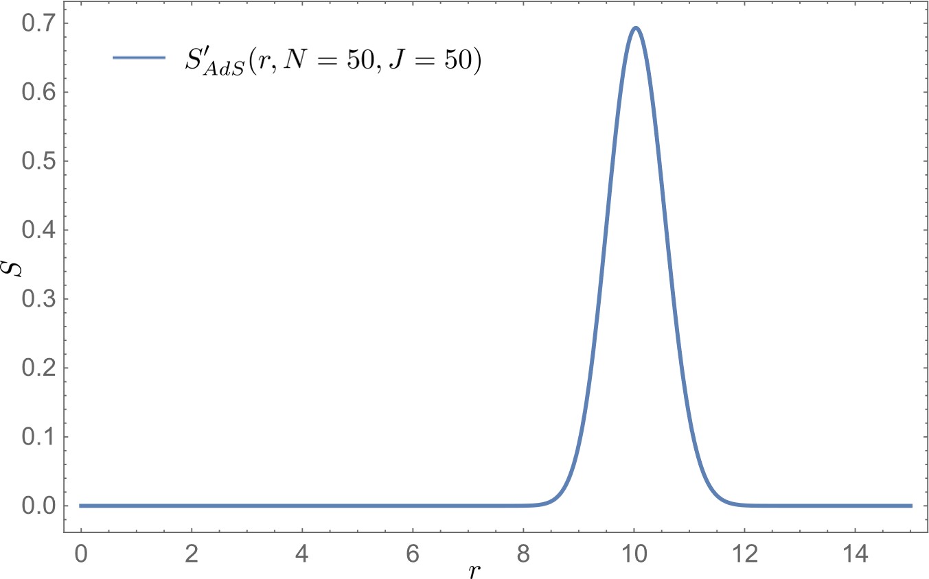
Figure 4: $S_{AdS}^{\prime}=S_{AdS}(r,50,50)-S_{0}(r,50)$ is plotted against $r$.

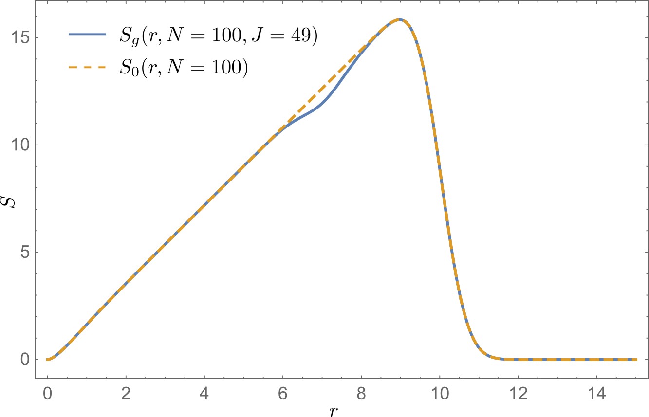
Figure 5: The solid line represents the target space entanglement entropy for the state corresponding to the giant graviton $S_{g}(r)$ with $N=100$ and $J=49$, while the dashed line represents the target space entanglement entropy for the ground state $S_{0}$ with $N=100$.

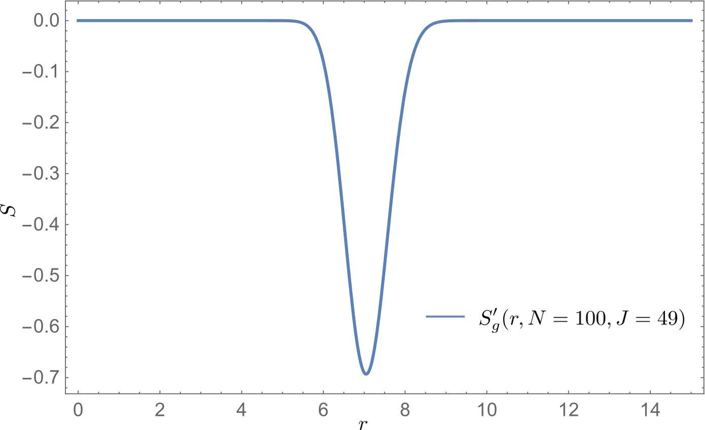
Figure 6: $S_{g}^{\prime}=S_{g}(r,100,49)-S_{0}(r,100)$ is plotted against $r$.

4 Area of boundary in the bubbling AdS geometry

In this section, we calculate the area (length) of boundary of the subregion $A$ in the bubbling geometry for the three cases, $AdS_{5}\times S^{5}$, an AdS giant graviton and a giant graviton.

We introduce the polar coordinates $(\tilde{r},\phi)$ in the $x_{1}-x_{2}$ plane. The solution determined by a droplet in Fig. 1 corresponding to $AdS_{5}\times S^{5}$ is given by [14]

$$\tilde{z}(\tilde{r},y;r_{0}) \equiv z-\frac{1}{2}=\frac{\tilde{r}^{2}-r_{0}^{2}+y^{2}}{2\sqrt{(\tilde{r}^{2}+r_{0}^{2}+y^{2})^{2}-4\tilde{r}^{2}r_{0}^{2}}}-\frac{1}{2}\ ,$$

$$V_{\phi} =-\frac{1}{2}\left(\frac{\tilde{r}^{2}+r_{0}^{2}+y^{2}}{\sqrt{(\tilde{r}^{2}+r_{0}^{2}+y^{2})^{2}-4\tilde{r}^{2}r_{0}^{2}}}-1\right)\ ,$$ (4.1)

where $r_{0}$ is related to the radius of $AdS_{5}$ as $r_{0}=R^{2}_{AdS}=\sqrt{N}$.

Based on (4.1), one can construct a solution for a general circular symmetric droplet as [14]

$$\tilde{z}=\sum_{i}(-1)^{i+1}\tilde{z}(\tilde{r},y;r_{i}),\ V_{\Phi}=\sum_{i}(-1)^{i+1}V_{\phi}(\tilde{r},y;r_{i})\ ,$$ (4.2)

where $r_{1}$ is the radius of the most outer circle and $r_{2}$ is the radius of the second outer circle and so on. We can construct $z$ corresponding to the droplets in Fig. 1 and Fig. 1 using (4.2).

We identify the target space of the complex matrix model with the $x_{1}-x_{2}$ plane at $y=0$ and consider the subregion $A$ in the $x_{1}-x_{2}$ plane. We calculate the area (length) of boundary of $A$ using the metric (2.12).

The induced metric in the $x_{1}-x_{2}$ plane at $y=0$ denoted by $\gamma_{ij}$ is

$$\gamma_{\tilde{r}\tilde{r}}=h^{2},\ \gamma_{\phi\phi}=-h^{-2}V_{\phi}^{2}+h^{2}\tilde{r}^{2},\ \gamma_{\tilde{r}\phi}=\gamma_{\phi\tilde{r}}=0\ .$$ (4.3)

Then , the area (length) of the boundary of $A$ in the $x_{1}-x_{2}$ plane, which we denote by $L$, is given by

$$L(r)=\int_{0}^{2\pi}d\phi\sqrt{\gamma_{\phi\phi}}=2\pi\sqrt{-h^{-2}V_{\phi}^{2}+h^{2}r^{2}}\ ,$$ (4.4)

where $h$ and $V_{\phi}$ are defined in (2.13).

First, we calculate the area of boundary of $A$ for $AdS_{5}\times S^{5}$. We see from (4.1) that $\gamma_{\phi\phi}$ is in the $y\rightarrow 0$ limit given by

$$\gamma_{\phi\phi} =\lim_{y\rightarrow 0}(-h^{-2}V_{\phi}^{2}+h^{2}\tilde{r}^{2})=\frac{\tilde{r}^{2}+r_{0}^{2}-|\tilde{r}^{2}-r_{0}^{2}|}{2r_{0}}\ .$$ (4.5)

Thus, the length of the boundary of $A$ is

$$L(r)=\int_{0}^{2\pi}\sqrt{\gamma_{\phi\phi}}=\sqrt{2}\pi\sqrt{\frac{r^{2}+r_{0}^{2}-|r^{2}-r_{0}^{2}|}{r_{0}}}\ .$$ (4.6)

$L$ is proportional to $r$ for $r<r_{0}$: $L(r)=\sqrt{\frac{2}{r_{0}}}\pi r$. This behavior qualitatively agrees with that of the target space entanglement entropy in Fig. 2. $L$ is constant for $r>r_{0}$,: $L(r)=\sqrt{2r_{0}}\pi$.

Next, we calculate the area of the boundary of $A$ for the (AdS) giant gravitons. We see from (4.1) and (4.2) that

$$z =\tilde{z}+\frac{1}{2}=\sum_{i=1}^{3}(-1)^{i+1}\tilde{z}(r,y;r_{i})+\frac{1}{2}\ ,$$

$$V_{\phi} =\sum_{i=1}^{3}(-1)^{i+1}V_{\phi}(r,y;r_{i})\ ,$$ (4.7)

where $r_{1}>r_{2}>r_{3}$. By using (4.3), we can calculate $\gamma_{\phi\phi}$ in the $y\rightarrow 0$ limit. The results are summarized in appendix B. We denote the area of boundary of $A$ for $AdS_{5}\times S^{5}$, an AdS giant graviton and a giant graviton by $L_{0}(r)$. $L_{AdS}(r)$ and $L_{g}(r)$, respectively.

In Fig. 7, we plot $L_{AdS}(r)$ for $r_{1}=\sqrt{101},r_{2}=10,r_{3}=\sqrt{50}$ and $L_{0}(r)$ for $r_{0}=r_{3}$ against $r$. As in the target space entanglement entropy, we subtract $L_{0}$ from $L_{AdS}$. In Fig .8, we plot $L_{AdS}^{\prime}=L_{AdS}(r)-L_{0}(r)$ against $r$. We see that $L_{AdS}^{\prime}$ has a peak around $r=r_{1}=\sqrt{N}$. This behavior of $L_{AdS}^{\prime}$ qualitatively agrees with $S_{AdS}^{\prime}$ in Fig. 4.

In Fig. 9, we plot $L_{g}(r)$ for $r_{1}=\sqrt{101},r_{2}=\sqrt{51},r_{3}=\sqrt{50}$ and $L_{0}$ for $r_{0}=r_{1}$ against $r$. In Fig. 10, we plot $L_{g}^{\prime}=L_{g}(r)-L_{0}(r)$ against $r$. We see that $L_{g}^{\prime}$ has a peak around $r=r_{2}=\sqrt{N}$. The sign of the peak is different from that of the peak in Fig. 6.: the area of boundary of $A$ has a positive peak, while the target space entanglement entropy a negative peak. The peak of the target space entanglement for the giant graviton comes from disappearance of a fermion. If we reinterpret this as a particle corresponding to a hole, the sign of the peak should flip.

In this way, we find that the contribution of the (AdS) giant gravitons to the area (length) of boundary of $A$ qualitatively agrees with that to the target space entanglement entropy.

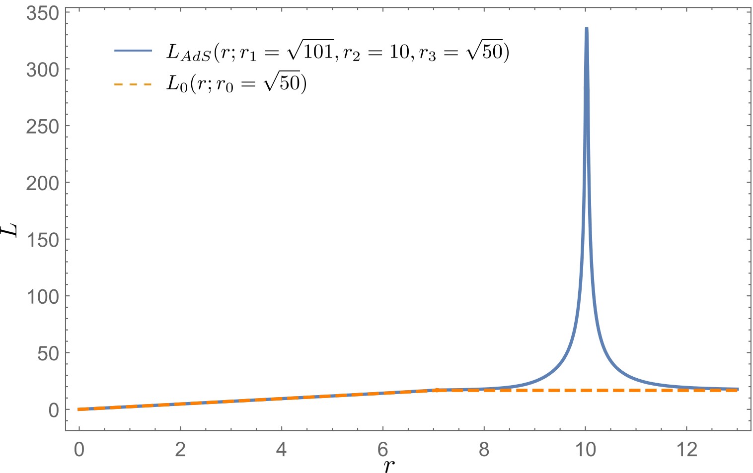
Figure 7: The solid line represents the area of the boundary of the subregion $A$ for an AdS giant graviton $L_{AdS}$ with $r_{1}=\sqrt{101},r_{2}=10$ and $r_{3}=\sqrt{50}$, while the dashed line represents that for the ground state $L_{0}$ with $r_{0}=\sqrt{50}$.

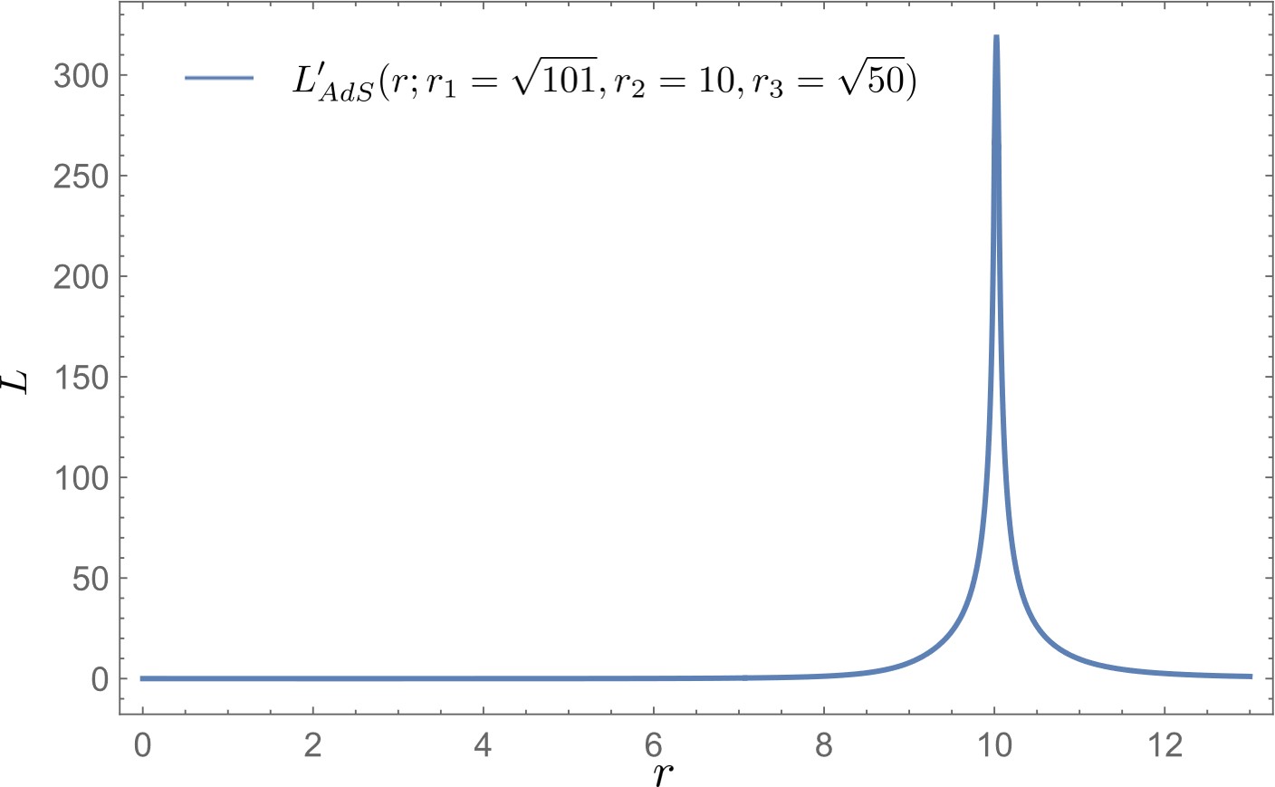
Figure 8: $L_{AdS}^{\prime}=L_{AdS}(r)-L_{0}(r)$ is plotted against $r$.

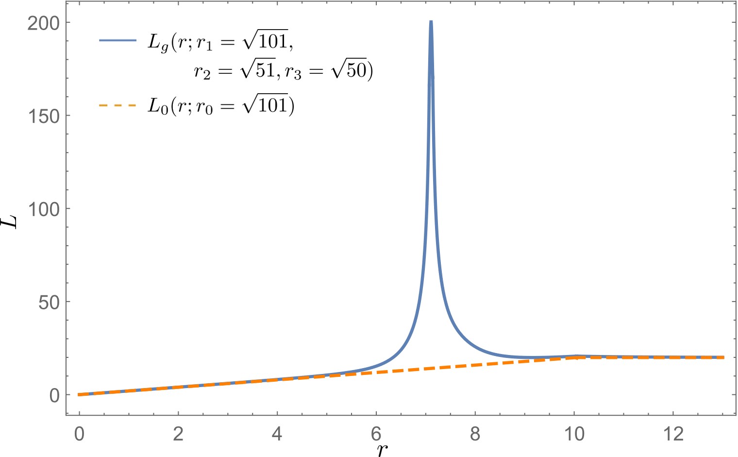
Figure 9: The solid line represents the area of boundary of subregion $A$ for a giant graviton $L_{AdS}$ with $r_{1}=\sqrt{101},r_{2}=\sqrt{51}$ and $r_{3}=\sqrt{50}$, while tha dashed line represents that for the ground state $L_{0}$ with $r_{0}=\sqrt{101}$.

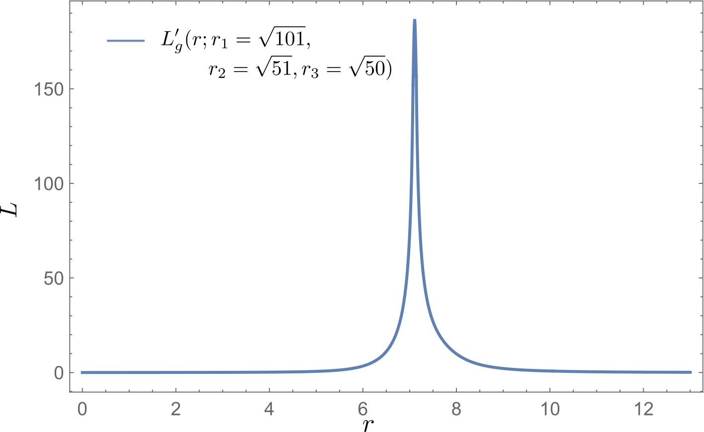
Figure 10: $L_{g}^{\prime}=L_{g}(r)-L_{0}(r)$ is plotted against $r$.

5 Conclusion and discussion

In this paper, we studied the target space entanglement entropy in the complex matrix model that describes the chiral primary sector in $\mathcal{N}=4$ SYM on $R\times S^{3}$. The eigenvalues of the complex matrix model are identified with the position coordinates of fermions in two-dimensional plane, and the eigenvalue distribution gives a droplet formed by the fermions, which is identified with that in the bubbling geometry specifying a boundary condition for a half-BPS solution with $R\times SO(4)\times SO(4)$ in type IIB supergravity. We calculated the target space entanglement entropy of a subregion in two-dimensional plane with droplets corresponding to $AdS_{5}\times S^{5}$, an AdS giant graviton and a giant graviton in the bubbling geometry. We also calculated the area of boundary of the subregion in the bubbling geometry, and found a qualitative agreement between the target space entanglement entropy and the area of boundary. For the following reason, it is considered as reasonable that we subtracted the contribution of the ground state ($AdS_{5}\times S^{5}$) when we compared the target space entanglement entropy and the area of boundary for the (AdS) giant gravitons. The fermions forming the droplet corresponding to the ground state originate from D3-branes in flat space-time. These D3-branes disappear, and their presence is trade for a deformation of flat space-time to $AdS_{5}\times S^{5}$. The target space entanglement entropy for the ground state measures the entanglement among the fermions corresponding to the disappearing D3-branes.

In order to see whether a quantitative agreement exists, we need to identify the effective Newton constant in (2+1)-dimensional space-time consisting the two-dimensional plane and the time and fix the factor of proportionality $1/4G_{N}$ between the target space entanglement entropy and the area. Possibly, we also need more elaborated correspondence between chiral primary states and droplets. Finally, we make comments on the scaling with respect to $N$. The maximum of the target space entanglement entropy of a subregion in two-dimensional plane with a droplet corresponding to $AdS_{5}\times S^{5}$ scales almost as $N^{1/2}$ as seen in Fig. 2, while the maximum of the magnitude of the subtracted one corresponding to an AdS giant graviton or a giant graviton scales as $N^{0}$. On the other hand, we see from (4.6) that the maximum of the area of boundary for $AdS_{5}\times S^{5}$ scales as $\sqrt{r_{0}}\sim N^{1/4}$, and we have verified that the maximum of the subtracted one for an AdS giant graviton or a giant graviton behaves almost as $N^{3/4}$ when the ratio between $r_{2}$ and $r_{3}$ for an AdS giant graviton in Fig. 1 and $r_{1}$ and $r_{2}$ for a giant graviton in Fig. 1 is fixed. This difference of the relative ratios between the maxima for $AdS_{5}\times S^{5}$ and (AdS) giant gravitons does not matter if only subtracted quantities make physical sense as discussed above. The fact that the entanglement entropy and the area scales as $N^{0}$ and $N^{3/4}$, respectively, commonly for an AdS giant gravion and a giant graviton suggests that the difference between the scalings of the subtracted entropy and area can be compensated by the scaling of the effective Newton constant. While it is conjectured in [3, 4] that the target space entanglement entropy in 9+1 dimensions scales as $N^{2}$, the target space entanglement entropy calculated in this paper is defined in a (2+1)-dimensional subspace so that it possibly scales in a different manner. We hope to report progress in these issues in the near future.

Appendix A Harmonic oscillator in two-dimensional plane

In this appendix, we review that the wave function of the lowest Landau level arises as a wave function of holomorphic sector of a particle under harmonic oscillator potential in two-dimensional plane.. The hamiltonian is represented in the complex coordinate $(z,z^{*})$ basis as

$$\hat{h}=-\frac{\partial}{\partial z}\frac{\partial}{\partial z^{*}}+zz^{*}=\hat{c}^{\dagger}_{1}\hat{c}_{1}+\hat{c}^{\dagger}_{2}\hat{c}_{2}+1\ ,$$ (A.1)

where

$$\hat{c}_{1}\equiv\frac{1}{\sqrt{2}}\left(z+\frac{\partial}{\partial z^{*}}\right),\;\;\hat{c}_{2}=\frac{1}{\sqrt{2}}\left(z^{*}+\frac{\partial}{\partial z}\right)$$

$$\hat{c}^{\dagger}_{1}\equiv\frac{1}{\sqrt{2}}\left(z^{*}-\frac{\partial}{\partial z}\right),\;\;\hat{c}^{\dagger}_{2}=\frac{1}{\sqrt{2}}\left(z-\frac{\partial}{\partial z^{*}}\right)$$ (A.2)

The commutation relations of $\hat{c}_{i}$ and $\hat{c}_{i}^{\dagger}$ are given by

$$[\hat{c}_{i},\hat{c}^{\dagger}_{j}]=\delta_{ij},\;\;[\hat{c}_{i},\hat{c}_{j}]=[\hat{c}^{\dagger}_{i},\;\;\hat{c}^{\dagger}_{j}]=0$$ (A.3)

The wave function of the ground state, $\Phi_{0,0}(z,z^{*})$, satisfies $\hat{c}\Phi_{0,0}=0$, which gives

$$\Phi_{0,0}=\frac{1}{\sqrt{\pi}}e^{-zz^{*}}\ .$$ (A.4)

The wave functions of excited states are given by

$$\Phi_{k,l}(z,z^{*})=\frac{1}{\sqrt{k!l!}}(\hat{c}^{\dagger}_{1})^{k}(\hat{c}^{\dagger}_{2})^{l}\Phi_{0,0}\ .$$ (A.5)

The energy eigenvalue of the above states are $k+l+1$. In particular, the wave functions of the $(0,l)$ excited states, $\Phi_{l}(z,z^{*})\equiv\Phi_{0,l}(z,z^{*})$, take a holomorphic form

$$\Phi_{l}(z,z^{*})=\sqrt{\frac{2^{l}}{l!\pi}}z^{l}e^{-zz^{*}}\ .$$ (A.6)

$\Phi_{l}(z,z^{*})$ are the wave functions of the lowest Landau level in the context of quantum Hall effect.

Appendix B $\gamma_{\phi\phi}$ for (AdS) giant gravitons

$\gamma_{\phi\phi}$ is given in the $y\rightarrow 0$ limit as follows:

(i) $r>r_{1}$

$$\lim_{y\rightarrow 0}\gamma_{\phi\phi}=\frac{r_{1}^{2}(r^{6}+r_{2}^{2}(r^{4}+3r_{3}\tilde{r}^{2})-r_{3}^{2}(4r^{4}+r_{2}^{4}))-r^{4}(\tilde{r}^{2}+r_{2}^{2})(r_{2}^{2}-r_{3}^{2})}{(\tilde{r}^{2}-r_{1}^{2})(\tilde{r}^{2}-r_{2}^{2})^{2}(\tilde{r}^{2}-r_{3}^{2})\sqrt{\frac{r_{1}^{2}}{(\tilde{r}^{2}-r_{1}^{2})^{2}}-\frac{r_{2}^{2}}{(\tilde{r}^{2}-r_{2}^{2})^{2}}+\frac{r_{3}^{2}}{(\tilde{r}^{2}-r_{3}^{2})^{2}}}}\ .$$ (B.1)

(ii) $r_{1}>r>r_{2}$

$$\lim_{y\rightarrow 0}\gamma_{\phi\phi}=\frac{-\tilde{r}^{2}(\tilde{r}^{2}+r_{3}^{2})(\tilde{r}^{2}(\tilde{r}^{2}-4r_{3}^{2})+r_{1}^{2}(r_{2}^{2}-r_{3}^{2})-r_{2}^{2}r_{3}^{2})}{(\tilde{r}^{2}-r_{1}^{2})(\tilde{r}^{2}-r_{2}^{2})(\tilde{r}^{2}-r_{3}^{2})^{2}\sqrt{{\frac{r_{1}^{2}}{(\tilde{r}^{2}-r_{1}^{2})^{2}}+\frac{r_{2}^{2}}{(\tilde{r}^{2}-r_{2}^{2})^{2}}-\frac{r_{3}^{2}}{(\tilde{r}^{2}-r_{3}^{2})^{2}}}}}\ .$$ (B.2)

(iii) $r_{2}>r>r_{3}$

$$\lim_{y\rightarrow 0}\gamma_{\phi\phi}=\frac{\tilde{r}^{2}r_{1}^{2}(r^{4}-\tilde{r}^{2}(r_{2}^{2}+r_{3}^{2})-3r_{2}^{2}r_{3}^{2})-r^{6}(r_{2}^{2}+r_{3}^{2})+4r^{4}r_{2}^{2}r_{3}^{2}-r_{1}^{4}(r_{2}^{2}r_{3}^{2}+r^{4})}{(\tilde{r}^{2}-r_{1}^{2})^{2}(\tilde{r}^{2}-r_{2}^{2})(\tilde{r}^{2}-r_{3}^{2})\sqrt{-\frac{r_{1}^{2}}{(\tilde{r}^{2}-r_{1}^{2})^{2}}+\frac{r_{2}^{2}}{(\tilde{r}^{2}-r_{2}^{2})^{2}}+\frac{r_{3}^{2}}{(\tilde{r}^{2}-r_{3}^{2})^{2}}}}\ .$$ (B.3)

(iv) $r_{3}>r$

$$\lim_{y\rightarrow 0}\gamma_{\phi\phi}=\frac{\tilde{r}^{2}(-r^{6}+\tilde{r}^{2}r_{2}^{2}(3\tilde{r}^{2}+r_{3}^{2})+(r_{2}^{2}-r_{3}^{2})(\tilde{r}^{2}+r_{2}^{2})-r_{2}^{4}(4\tilde{r}^{2}-r_{3}^{2}))}{(\tilde{r}^{2}-r_{1}^{2})(\tilde{r}^{2}-r_{2}^{2})^{2}(\tilde{r}^{2}-r_{3}^{2})\sqrt{\frac{r_{1}^{2}}{(\tilde{r}^{2}-r_{1}^{2})^{2}}-\frac{r_{2}^{2}}{(\tilde{r}^{2}-r_{2}^{2})^{2}}+\frac{r_{3}^{2}}{(\tilde{r}^{2}-r_{3}^{2})^{2}}}}\ .$$ (B.4)

References

- [1] S. Ryu and T. Takayanagi, Phys. Rev. Lett. 96, 181602 (2006) [arXiv:hep-th/0603001 [hep-th]].
- [2] E. A. Mazenc and D. Ranard, [arXiv:1910.07449 [hep-th]].
- [3] S. R. Das, A. Kaushal, G. Mandal and S. P. Trivedi, J. Phys. A 53, no.44, 444002 (2020) [arXiv:2004.00613 [hep-th]].
- [4] S. R. Das, A. Kaushal, S. Liu, G. Mandal and S. P. Trivedi, JHEP 04, 225 (2021) [arXiv:2011.13857 [hep-th]].
- [5] H. R. Hampapura, J. Harper and A. Lawrence, JHEP 10, 231 (2021) [arXiv:2012.15683 [hep-th]].
- [6] S. Sugishita, JHEP 08, 046 (2021) [arXiv:2105.13726 [hep-th]].
- [7] A. Frenkel and S. A. Hartnoll, [arXiv:2111.05967 [hep-th]].
- [8] T. Banks, W. Fischler, S. H. Shenker and L. Susskind, Phys. Rev. D 55, 5112-5128 (1997) [arXiv:hep-th/9610043 [hep-th]].
- [9] J. M. Maldacena, Adv. Theor. Math. Phys. 2, 231-252 (1998) [arXiv:hep-th/9711200 [hep-th]].
- [10] S. S. Gubser, I. R. Klebanov and A. M. Polyakov, Phys. Lett. B 428, 105 (1998) [hep-th/9802109].
- [11] E. Witten, Adv. Theor. Math. Phys. 2, 253 (1998) [hep-th/9802150].
- [12] S. Corley, A. Jevicki and S. Ramgoolam, Adv. Theor. Math. Phys. 5, 809-839 (2002) [arXiv:hep-th/0111222 [hep-th]].
- [13] D. Berenstein, JHEP 07, 018 (2004) [arXiv:hep-th/0403110 [hep-th]].
- [14] H. Lin, O. Lunin and J. M. Maldacena, JHEP 10, 025 (2004) [arXiv:hep-th/0409174 [hep-th]].
- [15] Y. Takayama and A. Tsuchiya, JHEP 10, 004 (2005) [arXiv:hep-th/0507070 [hep-th]].
- [16] A. Ghodsi, A. E. Mosaffa, O. Saremi and M. M. Sheikh-Jabbari, Nucl. Phys. B 729, 467-491 (2005) [arXiv:hep-th/0505129 [hep-th]].
- [17] I. Klich, J. Phys. A 39, L85-L92 (2006) [arXiv:quant-ph/0406068 [quant-ph]].
- [18] I. D. Rodriguez and G. Sierra, Phys. Rev. B 80, 153303 (2009) [arXiv:0811.2188 [cond-mat.mes-hall]].
- [19] P. Calabrese, M. Mintchev and E. Vicari, Phys. Rev. Lett. 107, 020601 (2011) [arXiv:1105.4756 [cond-mat.stat-mech]].