Surrogate-assisted distributed swarm optimisation for computationally expensive geoscientific models
Abstract
Evolutionary algorithms provide gradient-free optimisation which is beneficial for models that have difficulty in obtaining gradients; for instance, geoscientific landscape evolution models. However, such models are at times computationally expensive and even distributed swarm-based optimisation with parallel computing struggles. We can incorporate efficient strategies such as surrogate-assisted optimisation to address the challenges; however, implementing inter-process communication for surrogate-based model training is difficult. In this paper, we implement surrogate-based estimation of fitness evaluation in distributed swarm optimisation over a parallel computing architecture. We first test the framework on a set of benchmark optimisation problems and then apply it to a geoscientific model that features a landscape evolution model. Our results demonstrate very promising results for benchmark functions and the Badlands landscape evolution model. We obtain a reduction in computational time while retaining optimisation solution accuracy through the use of surrogates in a parallel computing environment. The major contribution of the paper is in the application of surrogate-based optimisation for geoscientific models which can in the future help in a better understanding of paleoclimate and geomorphology.
keywords:
Distributed evolutionary algorithms, Surrogate-assisted optimization, Bayesian optimisation, parallel computing, neuroevolution1 Introduction
Evolutionary algorithms are loosely motivated by the theory of evolution where species are represented by individuals in a population that compete and collaborate with each other, producing offspring over generations that to improve quality given by fitness measure [24, 45]. Particle swarm optimisation (PSO), on the other hand, is motivated by the flocking behaviour of birds or swarms represented by a population of particles (individuals) that compete and collaborate over time [1, 26, 27, 35]. Evolutionary and swarm optimisation methods have been prominent in a number of areas such as real-parameter global optimization, combinatorial optimization and scheduling, and machine learning [47, 53, 49, 1]. Research in evolutionary and swarm optimisation has focused on different ways to create new solutions with mechanisms that are heuristic in nature; hence, different variants are available [42, 26]. A major challenge has been in applying them in large-scale or computationally expensive optimisation problems that require thousands of function evaluations where a single function evaluation can take minutes to hours, or even days [33]. An example of an expensive function is a geoscientific model for landscape evolution problem [12], and deep learning models for big data problems [79]. Computationally expensive optimisation can be addressed with distributed/parallel computing and swarm optimisation [6, 62, 3]; however, we need efficient strategies for representing the problem.
Surrogate-assisted optimisation [31, 40, 52, 81, 30] provides a remedy for expensive models with the use of statistical and machine learning models to provide a low computational replicate of the actual model. The surrogate model is developed by training from available data generated during optimisation that features a set of inputs (new solutions) and corresponding output (fitness) given by the actual model. The method is also known as Bayesian optimisation where the surrogate model (acquisition function) is typically a Gaussian process model [10]; however, neural networks and other machine learning models have also been used [60]. Evolutionary and swarm optimization methods have been used in surrogate-assisted and Bayesian optimization, and have been prominent in fields of engine and aerospace design [51, 37, 58, 31], robotics [10], experimental design [29], and machine learning [63, 60].
Although limited studies exist, surrogate-assisted optimisation has been applied to geoscience problems. Wang et al. [71] presented reliability-enhanced surrogate-assisted PSO in landslide displacement prediction where the method was used for feature selection and hyperparameter optimization. The PSO-based surrogate model was used to search the hyperparameters and feature sets in the long short-term memory (LSTM) deep learning model for predicting landslide displacement. Gong et al. [28] presented an ensemble-based surrogate-assisted cooperative PSO for water contamination source identification. Zhou et al. [80] used a surrogate-assisted evolutionary algorithm that incorporated multi-objective optimization for oil and gas reservoirs focusing on good placement and hydraulic fracture parameters. The method employed global–local hybridization searching strategy via PSO with low-fidelity surrogate model that used a multilayer perception. Furthermore, Zhand et al. [78] used surrogate-assisted PSO for gas hydrate reservoir development. Wang et al. [72] presented a surrogate-assisted model for the optimization of hyperspectral remote sensing images. Chen et al. [22] utilised a surrogate-assisted evolutionary algorithm for heat extraction optimization of enhanced geothermal systems.
Evolutionary algorithms provide gradient-free optimisation which is beneficial for models that do not have gradient information, for instance, landscape evolution models [18, 12]. Some instances of such models are so expensive that even distributed evolutionary algorithms with the power of parallel computing would struggle. Hence, we need to incorporate efficient strategies such as surrogate-assisted optimisation that further improves their performance, but this becomes a challenge given parallel processing and inter-process communication for implementing surrogate estimation.
Landscape evolution models are geoscientific models that can be used to reconstruct the evolution of the Earth’s landscape over tens of thousands millions of years [23, 20, 8, 48, 7]. These models guide geologists and climate scientists in better understanding Earth’s geologic and climate history that can further also help in foreseeing the distant future of the planet [8, 64]. These models use data from geological observations such as bore-hole data and estimated landscape topography millions of years ago and require climate conditions and geological parameters that are not easily known. Hence, it becomes an optimisation problem to estimate these parameters which has been tackled mostly with Bayesian inference via Markov Chain Monte Carlo (MCMC) sampling in previous studies that used parallel computing [18], and surrogate assisted Bayesian inference [13]. Motivated by these studies, we bring the problem of the landscape evolution model to the evolutionary and swarm optimisation community; rather than viewing it as an inference problem, we view it as an optimisation problem.
In this paper, we implement a surrogate-based optimisation framework via swarm optimisation over a parallel computing architecture. We apply the framework for benchmark optimisation functions and a selected landscape evolution model. We investigate performance measures such as the accuracy of surrogate prediction given different types of problems that differ in terms of dimension and fitness landscape. The contribution of the paper is in the application of surrogate-based optimisation for geoscientific models using parallel computing. The estimation of parameters through surrogate-assisted estimation can in the future help in better understanding paleoclimate and geomorphology which can enhance knowledge about climate change.
The rest of the paper is organised as follows. Section 2 provides background and related work, while Section 3 presents the proposed methodology. Section 4 presents experiments and results and Section 5 concludes the paper with a discussion for future research.
2 Related work
2.1 Surrogate-assisted optimization
PSO has been continuously becoming prominent in surrogate-assisted optimisation. Yu et al. [76] compared surrogate-assisted hierarchical PSO, standard PSO, and a social learning PSO for selected benchmark functions under a limited computational budget. Li et al. [44] presented a surrogate-assisted PSO for computationally expensive problems where two criteria were applied in tandem to select candidates for exact evaluations. These included a performance-based criterion and a distance-based criterion used to enhance exploration that does not consider the fitness landscape of different problems. The results demonstrated better performance over several state-of-the-art algorithms for selected benchmark functions and a propeller design problem. Chen et al. [21] presented a hierarchical surrogate-assisted differential evolution algorithm for high-dimensional expensive optimization problems with RBF network for selected benchmark functions and an oil reservoir production optimization problem. Yi et al. [75] presented an online variable-fidelity surrogate-assisted harmony search algorithm with a multi-level screening strategy that showed promising performance for expensive engineering design optimization problems.
Furthermore, Li et al. [43] presented an ensemble of surrogates assisted PSO of medium-scale expensive problems which used multiple trial positions for each particle and selected the promising positions by using the superiority and uncertainty of the ensemble simultaneously. In order to feature faster convergence and to avoid wrong global attraction of models, the optima of two surrogates that featured polynomial regression and RBF models were evaluated in the convergence state of particles. Liao et al. [46] presented multi-surrogate multi-tasking optimization of expensive problems to accelerate the convergence by regarding the two surrogates as two related tasks. Therefore, two optimal solutions found by the multi-tasking algorithm were evaluated using the real expensive objective function, and both the global and local models were updated until the computational budget was exhausted. The results indicated competitive performance with faster convergence that scaled well with an increase in problem dimension for solving computationally expensive single-objective optimization problems. Dong et al. [25] presented surrogate-assisted black wolf optimization for high-dimensional and computationally expensive black-box problems that featured RBF-assisted meta-heuristic exploration. The RBF featured knowledge mining that includes a global search carried out using the black wolf optimization and a local search strategy combining global and multi-start local exploration. The method obtained superior computation efficiency and robustness demonstrated by comparison tests with benchmark functions. Chen et al. [21] presented efficient hierarchical surrogate-assisted differential evolution for high-dimensional expensive optimization using global and local surrogate models featuring RBF network with an application to an oil reservoir production optimization problem. The results show that the method was effective for most benchmark functions and gave a promising performance for a reservoir production optimization problem. Ji et al. [38] presented a dual-surrogate-assisted cooperative PSO for expensive multimodal problems which reported highly competitive optimal solutions at a low computational cost for benchmark problems and a building energy conservation problem. Ji et al. [39] further extended their previous approach using multi-surrogate-assisted multitasking PSO for expensive multimodal problems.
2.2 Landscape evolution models and Bayeslands
Landscape evolution models (LEMs) use different climate and geophysical aspects such as tectonics or climate variability [73, 65, 55, 11, 2] and combine empirical data and conceptual methods into a set of mathematical equations that form the basis for driving model simulation. Badlands (basin and landscape dynamics) [55, 56] is a LEM that simulates landscape evolution and sediment transport/deposition [34, 32] with an initial topography exposed to climate and geological factors over time with given conditions (parameters) such as the precipitation rate and rock erodibility coefficient. The major challenge is in estimating the climate and geological parameters and those that are linked with the initial topography since they can range millions of years in geological timescale depending on the problem. A way is to develop an optimisation framework that utilizes limited data. Since gradient information is not available, Badlands can be seen as a black-box optimisation model where the unknown parameters need to be found via optimisation or Bayesian inference. So far, the problem has been approached with Bayesian inference that employs MCMC sampling for the estimation of these parameters in a framework known as Bayeslands [14].
The Bayeslands framework had limitations due to the computational complexity of the Badlands model; hence, in our earlier works, we extended it using parallel tempering MCMC [19] that featured parallel computing to enhance computational efficiency. Although we used parallel computing with a small-scale synthetic Badlands model, the procedure remained computationally challenging since thousands of samples were drawn and evaluated. Running a single large-scale real-world Badlands model can take several minutes to hours, and even several days depending on the area covered by the landscape evolution model considered, and the span of geological time considered in terms of millions of years. Therefore, parallel tempering Bayeslands was further enhanced through surrogate-assisted estimation. We used developed surrogate-assisted parallel tempering MCMC for landscape evolution models where a global-local surrogate framework utilised surrogate training in the main process that managed MCMC replicas running in parallel [13]. We obtained promising results, where the prediction performance was maintained while lowering the overall computational time.
3 Surrogate-assisted distributed swarm optimisation
3.1 PSO
PSO is a population-based metaheuristic that improves the population over iterations with a given measure of accuracy known as fitness [41]. The population of the candidate solution is known as a swarm while the candidate solutions are known as particles that get updated according to the particle’s position and velocity. In the swarm, each particle’s movement is typically influenced by its local best-known position which gets updated when better positions are discovered by other particles. Equations 1 and 2 show the velocity and position update of the particle in a swarm, respectively.
| (1) |
| (2) |
where represent the velocity and position of a particle at time step , respectively. and are the user-defined cognitive and social acceleration coefficients, respectively. and are random numbers drawn from uniform distribution, and is a user-defined inertia weight. There are several variants in the way the particles get updated which have their strengths and limitations for different types of problems [41, 61, 68, 77, 74, 35].
3.2 Surrogate assisted Distributed framework
We update the swarm using the canonical particle update method [41] and execute the swarms in a distributed swarm framework that employs parallel computing.
3.2.1 Inter-process Communication
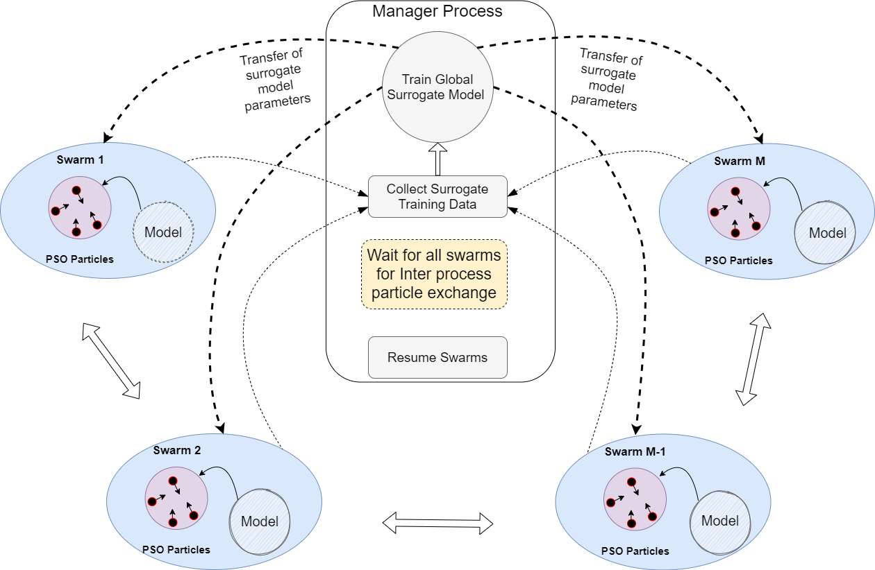
In our framework, we exchange selected swarm particles after a certain number of generations with inter-process communication. During the exchange, we replace 20 percent of the weaker particles with stronger ones from other swarms. This enhances the exploration and exploitation properties of our framework for the optimization problem. Afterwards, the process continues where local swarms create particles with new positions and velocities as shown in Figure 1. Hence, we feature distributed swarms and parallel processing for better diversity and computational complexity. We execute distinct parallel processes for respective swarms with central processing units (CPUs). Each process features the optimisation function which is either a synthetic problem made to be computationally expensive using time delay, or an application problem.
3.2.2 Surrogate Model
Suppose that the true function (model) is represented as ; where is the function and is a solution or particle from a given swarm. Our surrogate model outputs pseudo-fitness that would give an approximation of the true function via ; where, represents the difference between the surrogate and true function. The surrogate model gives an estimate using the pseudo-fitness for replacing the true function when required by the framework.
is an important hyperparameter that controls the use of a surrogate in the prediction. We do not want it to be too high in case we are not very confident, i.e. when enough data is not present for our surrogate model. We do not want it to be too low since the entire optimisation process will become time-consuming; hence, we need to tune this parameter. The surrogate model is trained by accumulating the data from all the swarms, i.e. the input and associated true-fitness pairs; where represents the particle and represents the swarm. In order to benefit from the surrogate model in the optimization process, it’s very crucial to manage the surrogate training and surrogate usage. We cannot use a surrogate from the very beginning of the optimization as its predictions will be random, and we also cannot wait too long as the computational efficiency will be affected. Hence, to manage the surrogate training and its use, an important hyperparameter is used which refers to the surrogate interval measured in terms of the number of generations. is the interval from which the collected data is used to train the model. The updated surrogate model is used until the next interval is reached, and knowledge in the surrogate model is refined in the next stage (defined by ) – this can be seen as a form of transfer learning. The collected input features () combined with the true fitness , create for the surrogate model.
| (3) |
where represents the given particle from the swarm, , is the output from the true fitness, and is the number of swarms. Therefore, the surrogate training dataset () is made up of input features () and response () for the particles that get collected in each surrogate interval (). The pseudo-fitness is given by .
3.2.3 Surrogate-assisted Framework
In Algorithm 1, we present further details about our framework that features surrogate-assisted optimisation using distributed swarms.
We implement the algorithm using distributed computation over CPU cores, as shown in Algorithm 1. The manager process is shown in black where inter-process communication among swarms takes place which exchange parameters at regular intervals (given by ). Furthermore, the surrogate model is also trained at regular intervals (). The parallel swarms of the distributed framework have been highlighted in pink in Algorithm 1. Stage 0 features the initialization of particles in the swarm. We begin the optimisation process by initialising all the swarms (Stage 0.1) in the ensemble with random real numbers in a range as required by the optimisation function (model).
Once the swarms are initialised, we begin the evolution (optimisation) by first evaluating the particles in the swarms using the fitness (objective) function. Hence, we iterate over surrogate interval () and evolve each swarm for generations, both user-defined parameters. We update the best particle and best fitness for each of the respective swarms in the ensemble afterwards. Once these basic operations are done, we begin the evolution where we create a new set of swarms for the next generation by velocity and position update (Stage 1.1).
The crux of the framework is when we consider whether to evaluate the fitness function (true fitness) or to use the surrogate model of the fitness function (pseudo-fitness) when computing fitness values. Stage 1.2 shows how to update the fitness using either surrogate or true fitness of the particle depending on the interval and . Initially, this is not done until the very first surrogate interval is not reached, where all the fitness evaluations are from the true function. In Stage 1.3, we calculate the moving average of the past three fitness values for a particular particle by = mean() to combine with the surrogate model prediction (Stage 1.4). This is done so that we incorporate the recent history of the true model fitness, with the surrogate-based estimated fitness, which is motivated by the autoregressive moving average (ARMA) model. Note that if present, the surrogate estimation fitness will be also considered as part of the past three fitness values. In the case when surrogate fitness is included, we note that additional errors will be added; however, this will be further averaged with true values as there cannot be two surrogate fitness values. In Stages 1.5 and 1.6, we calculate actual fitness and save the values for future surrogate training. Our swarm particle update depends on and , and due to poor surrogate performance, some of the weaker particles can get higher fitness scores. In order to avoid this issue, we ensure that and are from true fitness evaluation. In Stage 2.1, given a regular interval ( generations), we prepare an exchange of selected particles with neighbouring swarms via elitism, where we replace a given percentage of weak particles (given by fitness values). is a user-defined parameter that determines how much of the swarm particles need to be exchanged. We have given recommendations for value in the design of experiments. We select only 20% of elitist values as we do not want the majority of the swarms to be similar and maintain diversity.
We note that before we consider the use of pseudo-fitness, we need to train the surrogate model with the same training data which is created from the true fitness. Hence, we need to collect the training data for the surrogate model from all the swarms in the ensemble. In Stage 3.0, the algorithm uses surrogate training data collected from Stage 1.6 ( as shown in Equation 3). In Stage 4, the algorithm trains the surrogate model in the manager process with data from Stage 3. The knowledge from the trained surrogate model is then used in the fitness estimation as shown in Stage 1.4. Stage 5.0 implements the termination condition where the algorithm signals the manager process to decrement the number of swarms alive (active) in order to terminate the swarm process. This is done when the maximum number of fitness evaluations has been reached () for the particular swarm. We use a neural network-based surrogate model with Adam optimisation [2]. In order to validate the performance of the algorithm, we measure the quality of the surrogate estimate using the root mean squared error (RMSE):
| (4) |
where and are the true and pseudo-fitness values, respectively. denotes the number of times the surrogate model is used for estimation. Figure 1 provides a visual description of the proposed algorithm where multiple swarms are executed using the manager process that also controls the particle exchange and surrogate model update.
![[Uncaptioned image]](/html/2201.06843/assets/alg.png)
4 Application: Landscape evolution models

Similar to optimizing mathematical functions, in certain problems, we are required to evaluate a score using some simulation or computationally expensive process, such as geoscientific models [48, 67, 20]. Landscape evolution models (LEMs) are a class of geoscientific models that evolve a given topography over a given time with given geological and climate conditions such as rock erodibility and precipitation [55]. LEMs are used to model and understand the landscape and basin evolution back in time over millions of years showing surface processes such as the formation of river systems and erosion/deposition, where there is movement of sediments from source (mountains) to sink (basins) [20]. LEMs help geologists and paleoclimate scientists understand the evolution of the planet and climate history over millions to billions of years; however, there are major challenges when it comes to data. LEMs generally require data regarding paleoclimate processes which is typically unavailable; and hence, we need to estimate them with methods such as MCMC sampling [17, 15]. There is limited work in the literature where optimisation methods have been used to estimate the unknown parameters for LEMs, which is the focus of this study. We note that typically, LEMs are computationally very expensive which is dependent on the resolution of the study area (points/kilometer) and the duration of evolution (simulation) back in time (millions of years). Hence, large scale study areas can take from hours to days to run a single LEM even with parallel computing [55]. There is no gradient information in the case of Badlands LEM used for this study, and hence estimating the model parameters is a challenge.
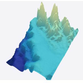
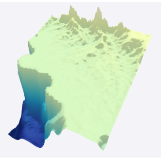
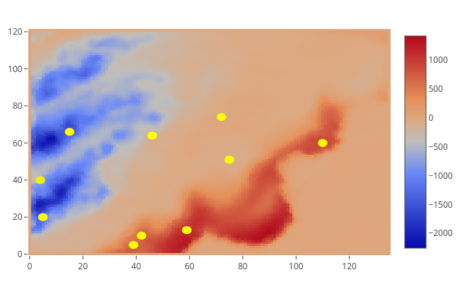
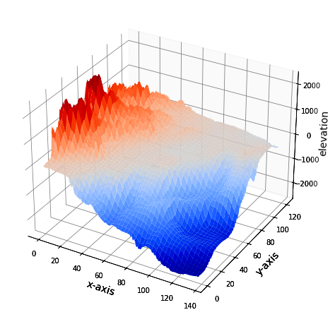
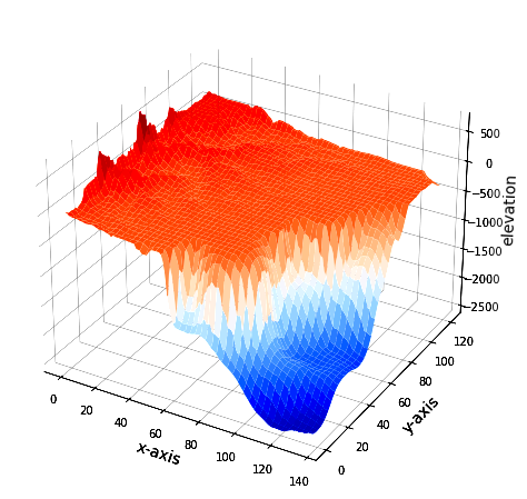
In order to demonstrate the optimisation procedure, we select problems where synthetic initial topography has been created using present day topography and used in our previous work [17, 15]. The selected LEM features a continental margin (CM) problem that is selected taking into account computational time of a single model run as it takes less than three seconds on a single central processing unit (CPU). The CM problem initial topography is selected from the present-day South Island of New Zealand as shown in Figure 2 which covers 136 by 123 kilometres. We provide a visualization of the initial and final topographies along with an erosion/deposition map for CM problem in Figure 3. The CM features six free parameters (Table 1). The notable feature of all three problems is that they model both elevation and erosion/deposition topography. We use the initial topography (Figure 3) and the true values given in Table 1, and run the Badlands LEM by simulating 1 million years to synthetically generate the ground-truth topography. We then create a fitness function with the ground-truth topography and set experiments so that the proposed optimisation methods can get back the true values. The details about the fitness function are given in the following section.
| Issue | Rainfall (m/a) | Erod. | n-value | m-value | c-marine | c-surface | Uplift (mm/a) |
|---|---|---|---|---|---|---|---|
| True-values | 1.5 | 5.0-e06 | 1.0 | 0.5 | 0.5 | 0.8 | - |
| Limits | [0,3.0 ] | [3.0-e06, 7.0-e06] | [0, 2.0] | [0, 2.0] | [0.3, 0.7] | [0.6, 1.0] | - |
4.1 Fitness function
The Badlands LEM produces a simulation of successive time-dependent topographies; however, only the final topography is used for topography fitness since no successive ground-truth data is available. The sedimentation (erosion/deposition) data is typically used to ground-truth the time-dependent evolution of surface process models that include sediment transportation and deposition [55, 14].
We adapt the fitness function from the likelihood function used in our previous work that used Bayesian inference via MCMC sampling for parameter estimation in Badlands LEM [17]. represents the vector of free parameters, such as precipitation rate and erodibility which are independent and optimised by our proposed algorithms based on PSO. The initial topography is given as a two-dimensional matrix , where corresponds to the location which is given by the latitude and longitude (Figure 2). Hence, our topography fitness function for the topography is given by computing that represents the final topology (at final time ) by Badlands LEM.
| (5) |
where, is the number of observations.
Badlands LEM produces a sediment erosion/deposition topography at each time frame. We use a selected vector of locations (Figure 3 - Panel c) at time () simulated (predicted) by the Badlands LEM for given . The sediment fitness is given below
| (6) |
The total fitness is the combination of the topography and sediment fitness. Note that the initial topography should not be confused with the initial state of the swarms of the PSO. The initial topography is simulated using pre-day topography of the region and hence not generated via any distribution.
5 Experiments and Results
In this section, we present the results of our framework on synthetic benchmark functions and Badlands LEM. The experiments consider a wide range of performance measures which includes optimization performance in terms of fitness score, computational time, and accuracy of the surrogate model.
5.1 Experiment design
We provide the experimental design and parameter setting for our experiment as follows. We implement distributed swarm optimization using parallel computing and inter-process communication where the swarms can have separate processes and exchange solutions (particles) with Python multi-processing library 111https://github.com/sydney-machine-learning/surrogate-assisted-distributed-swarms.
The synthetic benchmark optimisation functions are given in Equation 6 (Spherical), Equation 7 (Ackley), Equation 8 (Rastrigin), and Equation 9 (Rosenbrock). In Equation 7, we use the user-defined parameters, and . Similarly in Equation 8, and and are user-defined parameters. Note that these functions are chosen due to different levels of difficulty in optimisation and the nature of their fitness landscape. The Spherical function is considered to be a relatively easier optimisation problem since it does not have interacting variables. Ackley and Rastrigin are known to have many local minimums, while Rosenbrock is known as the valley-shaped function.
| (7) |
| (8) |
| (9) |
We use () swarms which run as parallel processes (swarms) that inter-communicate with each other at regular interval (). We use the same values for certain hyper-parameters ( and ) to simplify the algorithm. We exchange of a subset of particles (best 20% from the population) with the neighbouring island (worst 20% of the population). This is implemented by setting in Algorithm 1. We use the population size of 20 particles per swarm, the inertia weight with social and cognitive coefficients( and ). We determined these values for parameters in the trial experiments by taking into account the performance on different problems with a fixed number of evaluations. We use minimum and maximum bounds on the parameters as described in Table 1, respectively. We run experiments for 30 and 50 dimension (30D and 50D) instances of the respective benchmark problems. The dimension of our problem for synthetic functions (eg. Rosenbrock) is much larger than LEM since in the literature, 30D optimization functions are more common. We set the total number of function evaluations to 100,000 and 200,000, respectively. In the case of the Badlands model, we use 10,000 function (model) evaluations for the CM problem.
We used the PyTorch machine learning library 222PyTorch: https://pytorch.org/ for implementing the surrogate model that uses a neural network model with Adam learning. The surrogate neural network model architecture is given in Table 2, where the input dimensions are defined, i.e. 30D and 50D instances of the benchmark functions. In a similar way, we extend our approach for optimization in the Badlands model with the CM problem, featuring a 6-dimensional (6D) search space. The first and second hidden layers of the neural network-based surrogate model are shown in Table 2. We note that the output layer in the model for all the problems contains only one unit which provides the estimated fitness score.
| Problem | Hidden() | Hidden() | |
|---|---|---|---|
| Rosenbrock 30D | 30 | 15 | |
| Rastrigin 30D | 30 | 15 | |
| Ackley 30D | 30 | 15 | |
| Spherical 30D | 30 | 15 | |
| Rosenbrock 50D | 50 | 25 | |
| Rastrigin 50D | 50 | 25 | |
| Ackley 50D | 50 | 25 | |
| Spherical 50D | 50 | 25 | |
| Badlands | 20 | 10 |
5.2 Results for synthetic benchmark functions
We first present the results (fitness score) for different problems using serial (canonical) PSO, distributed PSO (D-PSO) and surrogate-assisted distributed swarm optimisation (SD-PSO) as shown in Table 3. We use a fixed surrogate probability () and present results featuring mean, standard deviation (std), and best and worst performance for over 30 independent experimental runs with different random initialisation in swarms as shown in Table 3. Note that lower fitness scores provide better performance.
We find a significant reduction in elapsed time for all the problems in Table 3. Note that we added a 0.05 seconds time delay to the respective problems in order to make them slightly computationally expensive to depict real-world application problems (models). When we consider serial PSO with D-PSO and SD-PSO in terms of optimisation performance given by the fitness score, we find that D-PSO improves the PSO significantly for 30D and 50D cases of Rosenbrock, Spherical and Rastrigin problems. We also see improvement in Ackley’s problem, but it’s not as large as in previous problems. We find the variation in the results given by the standard deviation is lowered highly with D-PSO which shows it is more robust to initialization and has the ability to provide a more definitive solution.
Moreover, in comparison of SD-PSO with D-PSO, we mostly get better fitness with SD-PSO, with a reduction of computation time due to the use of surrogates. Despite the use of surrogate-based fitness estimation, we observe that the fitness score has not greatly depreciated. It is interesting to note in Ackley 30 and 50D case, addition of surrogates improved the fitness score. We find a 30% reduction in computational time, it is expected this to increase if we had more time delay (rather than 0.05 seconds), which will be shown in the Badlands LEM experiments to follow.
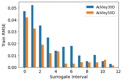
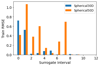
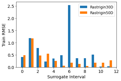
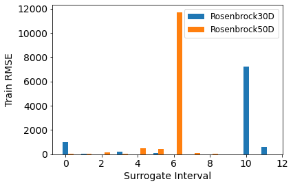
The RMSE of prediction of fitness by the surrogate model is shown in Table 4. We notice large RMSE values for the Rosenbrock problem when compared to the rest. In surrogate prediction accuracy (RMSE) given in Figure 5, we observe a constant reduction in RMSE with intervals (along the x-axis) in Ackley (30D and 50D), and Spherical (30D) model functions. In other problems, the RMSE is lower towards the end, but the trend is not that smooth. We note that in the Rosenbrock function, there exists an interval where our surrogate performs poorly causing a major decrease in accuracy.
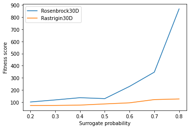
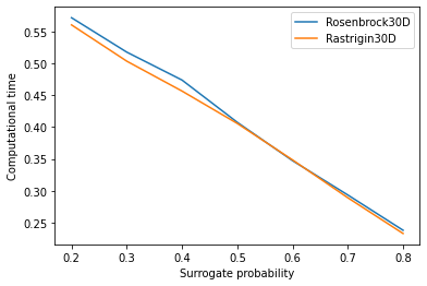
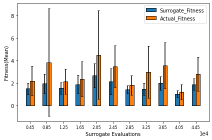
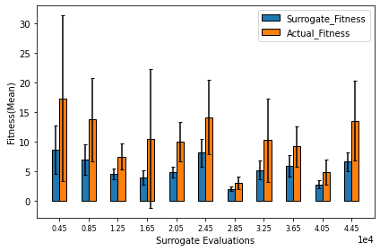
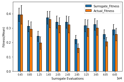
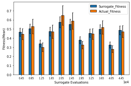
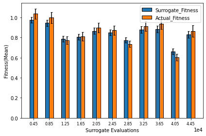
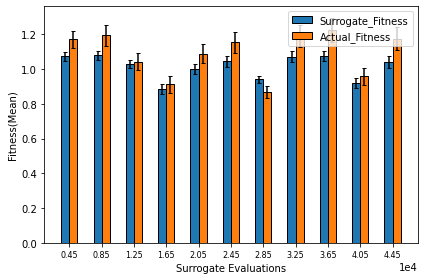
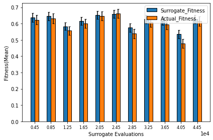
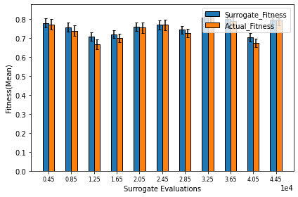
Figure 6 and 7 provide a visual description of surrogates prediction quality in the evolution process. We show the bar plots for mean values with a 95% confidence interval (shown by error bars) of the actual fitness and pseudo-fitness at regular intervals for different benchmark problems. We notice that the Rastrigin and Ackley problems have a better surrogate prediction with better confidence intervals when compared to the Spherical problem. Finally, we evaluate the effect of the surrogate probability for Rosenbrock and Rastrigin 30D problems. Figure 4 (Panel a) provides a graphical analysis of the effect of the fitness score and computational time (Panel b) given different surrogate probabilities. We observe that the computational time decreases linearly with an increase in the surrogate probability. On the other hand, the fitness score degrades with an increase of surrogate probability (Rosenbrock 30D); however, with an elbow-shaped curve – a trade-off can exist between time and optimization performance (surrogate probability of 0.6). In the case of the Rastrigin 30D, there is not a large difference in loss of fitness (surrogate probability 0.5) when compared to the Rosenbrock 30D; we note that these problems have distinctly different fitness landscapes which could explain about the difference in the performance.
| Problem | Method | Fitness Score | Elapsed Time |
|---|---|---|---|
| [mean std best worst] | (minutes) | ||
| Rosenbrock 30D | PSO | 183.95 109.94 60.88 455.01 | 84.39 |
| D-PSO | 108.78 38.0 55.0 178.0 | 11.22 | |
| SD-PSO (0.5) | 149.7 50.91 67.92 270.18 | 7.113 | |
| Rosenbrock 50D | PSO | 1285.41 559.54 432.89 2519.02 | 84.37 |
| D-PSO | 1269.03 390.0 78.0 2084.0 | 11.24 | |
| SD-PSO(0.50) | 2449.32 1093.8 685.48 5298.79 | 7.114 | |
| Spherical 30D | PSO | 9.06 9.22 1.43 37.85 | 84.35 |
| D-PSO | 4.79 3.0 1.0 12.0 | 11.31 | |
| SD-PSO | 1.82 0.74 0.9 3.33 | 7.112 | |
| Spherical 50D | PSO | 252.96 102.69 67.75 426.74 | 84.38 |
| D-PSO | 175.2 45.0 118.0 256.0 | 11.23 | |
| SD-PSO(0.50) | 111.85 48.36 34.05 239.828 | 7.113 | |
| Rastrigin 30D | PSO | 72.33 19.72 27.05 112.21 | 84.38 |
| D-PSO | 62.61 12.0 41.0 90.0 | 11.20 | |
| SD-PSO(0.50) | 77.23 12.57 52.96 107.26 | 7.113 | |
| Rastrigin 50D | PSO | 188.34 33.83 130.96 257.53 | 84.39 |
| D-PSO | 180.7 24.0 122.0 215.0 | 11.1 | |
| SD-PSO(0.50) | 243.73 25.1 192.2 307.82 | 7.114 | |
| Ackley 30D | PSO | 2.32 0.39 1.66 3.03 | 84.37 |
| D-PSO | 1.83 0.0 1.0 2.0 | 11.21 | |
| SD-PSO(0.50) | 1.66 0.33 0.99 2.24 | 7.112 | |
| Ackley 50D | PSO | 3.8 0.38 3.24 4.58 | 84.38 |
| D-PSO | 3.42 0.0 3.0 4.0 | 11.21 | |
| SD-PSO(0.50) | 3.34 0.23 2.76 3.73 | 7.113 |
| Problem | Surrogate Prediction RMSE | Surrogate Training RMSE |
|---|---|---|
| [mean std] | ||
| Rosenbrock 30D | 368.33 | 7.68e+02 1.97e+03 |
| Rosenbrock 50D | 284.73 | 1.09e+03 3.45e+03 |
| Spherical 30D | 0.44 | 1.20e-01 2e-01 |
| Spherical 50D | 0.61 | 7.10e-01 8.75e-01 |
| Rastrigin 30D | 0.46 | 2.88e-01 2.54e-01 |
| Rastrigin 50D | 0.54 | 7.33e-01 1.35e+00 |
| Ackley 30D | 0.08 | 1.15e-02 4.53e-03 |
| Ackley 50D | 0.08 | 1.25e-02 4.17e-03 |
| Badlands (CM) | 0.0218 | 2.59e-3 1.95e-3 |
5.3 Results for the Badlands model
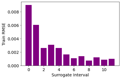
Finally, we present results for the case of the Badlands CM problem which is a 6D problem. The results for CM problem highlighting our methods (PSO, D-PSO and S-DPSO) when compared to previous approaches (PT-Bayeslands and SAPT-Bayeslands) are shown in Table 5. The results show the computational time and prediction performance of the Badlands model in terms of elevation and erosion/deposition RMSE (using Equations 4 and 5, respectively) given the optimised parameters. The results show the mean and standard deviation from 30 experimental runs from independent initial positions. We see a major reduction in computational time using D-PSO when compared to PSO and find consistent performance in terms of elevation and erosion RMSE. The experiments used a surrogate model at an interval of 10 generations with a probability of 0.5. We observe that the SD-PSO further improved the performance by reducing computational time using surrogates. The RMSE of the estimation of fitness function by the surrogate model when compared to the actual Badlands model is shown in Table 4. We note that the RMSE in this case cannot be compared to the synthetic fitness functions (eg. Rosenbrock) since the fitness function is completely different. In synthetic fitness functions, there is no data whereas in Badlands LEM, we use Badlands prediction and ground-truth topography data to compute the fitness. Figure 5 (Panel e) shows surrogate training accuracy (RMSE) for different surrogate intervals where we observe a constant improvement of performance by the surrogate model over time (surrogate intervals). This implies that the surrogate model is improving as it gathers more data over time.
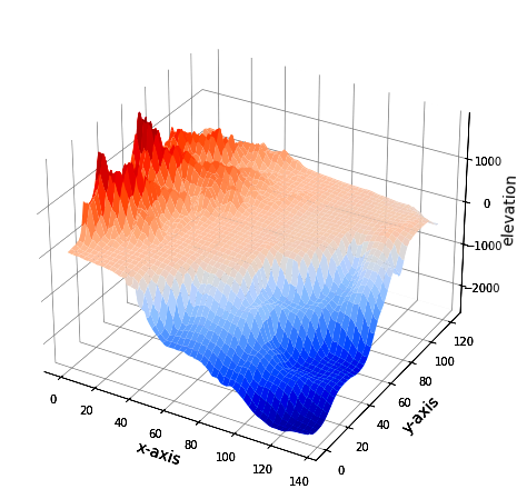
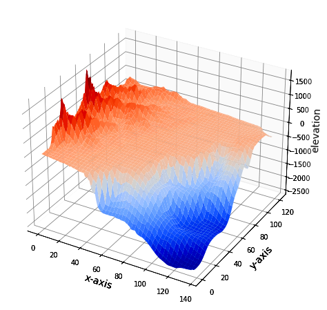
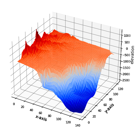
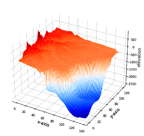
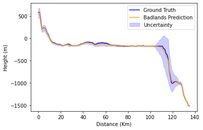
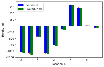
In Figure 8, we show the change in CM topology over selected time-slices simulated by Badlands according to the parameters optimized by S-DPSO. The elevation RMSE in Table 5 considers the difference between ground-truth topography given in Figure 3. We notice that visually the final topography (present-day) in Figure 8 (Panel f) resembles Figure 3 (Panel b). Furthermore, we show in Figure 9 a cross-section (Panel a) for Badlands predicted elevation vs the ground-truth elevation for final or present-day topography. We also show the bar plot (Panel b) of predicted vs ground-truth sediment erosion/deposition at 10 selected locations taken from Figure 3 (Panel c). The cross-section and bar plots show that the Badlands prediction well resembled the ground-truth data, respectively. We obverse that the cross-section (Panel a) uncertainty is higher for certain locations as highlighted. The high uncertainty is in an area of a high slope below sea level which is reasonable given the effect of sediment flow due to precipitation.
/
/
/
| Method | Elevation RMSE | Elevation RMSE | Erosion RMSE | Erosion RMSE | Time |
| (mean) | (std) | (mean) | (std) | (seconds) | |
| PT-Bayeslands [14], | 70.80 | 10.03 | 35.91 | 11.36 | 3243 |
| SAPT-Bayeslands [19] | 82.0 | 8.23 | 44.33 | 13.37 | 1859 |
| PSO | 60.93 | 3.56 | 18.47 | 4.12 | 18480 |
| D-PSO | 61.61 | 4.46 | 26.97 | 5.39 | 4020 |
| S-DPSO | 61.17 | 4.57 | 23.63 | 5.11 | 3462 |
6 Discussion
We note that the surrogate-assisted method (SD-PSO) estimates the fitness and the velocity update in the next generation as done in a standard PSO (Equations 1 and 2). The surrogate fitness does not change the structure of the PSO, it is only used as a way to estimate the fitness and hence reduce the computational time. We note that the performance of an optimisation method depends on the nature of the optimisation benchmark problems [36] due to their fitness landscape modality, i.e., unimodal (Rosenbrock, Sphere) and multimodal (Rastrigin, Ackley), and separability (Rosenbrock is considered non-separable and Sphere separable). It is easier to construct optimisation methods for separable functions using a divide and conquer approach, which faces challenges in separable problems [57, 16]. In terms of the results, we find that SD-PSO has done better than PSO and D-PSO (Table 3 and Table 5) for most problems. This could be done to the fitness estimation by the surrogate model, i.e. surrogate -based fitness estimations could have helped the algorithm in escaping local optima and hence it achieved better fitness. In general, the results show that distributed surrogate-assisted swarm optimisation framework can improve performance by decreasing computation time while retaining optimisation accuracy (fitness).
We highlight that the Badlands model does not provide gradient information regarding the parameters; and hence, only gradient-free optimisation and inference methods can be used. In our previous work, MCMC sampling (PT-Bayeslands and SAPT-Bayeslands [14, 19]) has been used, where the parameter inference was implemented via random-walk proposal distribution with MCMC replicas running in parallel. In this paper, the results show that the use of meta-heuristic (evolutionary) search operators from particle swarm optimisation provides better search features. The results motivate the use of the proposed methodology for expansive optimisation models, which can feature other geoscientific models. Further use of surrogates in larger instances of the Badlands LEM can provide a significant reduction in computational time.
A major contribution of the framework is in the implementation using parallel computing, which takes into account inter-process communication when exchanging particles (solutions) during the optimisation process. In our proposed framework, the surrogate training was implemented in the manager process and the trained parameters were transferred to the parallel swarm processes, where the local surrogate model was used to estimate the fitness of the particle when required (Figure 1). This implementation seamlessly updated the local surrogate model at regular intervals set by the user. We note that although less than eight parallel swarm processes were used, in large-scale problems, the same implementation can be extended and amended. We note that in the case when the number of parameters in the actual model significantly increases, different ways of training the surrogate model can be explored. We also note that the number of particles per swarm is strongly dependent upon the problem in hand [41, 35].
Another major contribution from the optimisation process for the case of the landscape evolution model is the estimation of the parameters, such as precipitation values in the Badlands model. We note that MCMC sampling methods provide inference whereas, optimisation methods provide an estimation of parameters. The major difference is that we represent the parameters using probability distribution in the case of inference, whereas optimisation methods provide single-point estimates. Through optimisation, we can estimate what precipitation values gave rise to the evolution of landscape which resulted in the present-day landscape. The landscape evolution model hence provides a temporal topography map of the geological history of the region under study. These topographical maps, along with the optimised values for geological and climate parameters (such as precipitation and erodibility) can be very useful to geologists and paleoclimate scientists.
Although PSO has been selected as the designated evolutionary optimisation algorithm, the framework has the flexibility to enable the implementation of other evolutionary algorithms depending on the application problem. A wide range of PSO variants exist in the literature with strengths and limitations [66, 70, 9]. In the case when the application involves combinatorial optimisation or a scheduling problem, then an appropriate evolutionary algorithm would be needed.
Our experiments considered a simulation where the present-day topography of a selected region was used as the initial topography. The Badlands model ran depicting a million years in time, to simulate successive topographies. However, in the area of LEMs, the focus is generally to understand the environmental and climate history back in time that led to present-day topography. In such cases, we need to estimate the initial topography (eg. a million years back in time), which can be based on present-day topography. The estimation of initial topography is an optimisation problem of its own and joint optimisation of parameters such as precipitation can make the process very complex. However, this can be addressed in future research.
7 Conclusions and Future Work
We presented a surrogate framework that features parallel swarm optimisation processes and seamlessly integrates surrogate training from the manager process to enable surrogate fitness estimation. Our results indicate that the proposed surrogate-assisted optimisation method significantly reduces the computational time while retaining solution accuracy. In certain cases, it also helps in improving the solution accuracy by escaping from the local minimum via the surrogates. Although we used PSO as the designated algorithm, other optimisation algorithms, such as genetic algorithms, evolution strategies, and differential evolution can also be used.
In future work, the parallel optimisation process could be improved by a combination of different optimisation algorithms which can provide different capabilities in terms of exploration and exploitation of the search space. The proposed framework can also incorporate other benchmark function models, particularly those that feature constraints and also be applied to discrete parameter optimisation problems which are expensive computationally.
8 Further Information
8.1 Ethical approval
The data used in the manuscript is openly available and does not need any ethical approvals.
8.2 Funding details
There are no external funding sources to report.
8.3 Conflict of interest
The authors do not have any conflict of interest with the manuscript and publication process.
8.4 Availability of data and materials
We provide an open-source implementation of the proposed algorithm in Python along with data and sample results 333Surrogate-assisted distributed evolutionary algo: https://github.com/sydney-machine-learning/surrogate-assisted-distributed-evo-alg.
8.5 Authorship Contribution
R. Chandra contributed by writing, coding, experiments and analysis of results. Y. Sharma contributed by coding, experiments, writing and analysis.
Acknowledgement
The authors would like to thank Ratneel Deo from the University of Sydney for his support during the initial phase of this research.
References
- Ab Wahab et al. [2015] Ab Wahab, M. N., Nefti-Meziani, S., Atyabi, A., 2015. A comprehensive review of swarm optimization algorithms. PloS one 10 (5), e0122827.
- Adams et al. [2017] Adams, J. M., Gasparini, N. M., Hobley, D. E. J., Tucker, G. E., Hutton, E. W. H., Nudurupati, S. S., Istanbulluoglu, E., 2017. The landlab v1.0 overlandflow component: a python tool for computing shallow-water flow across watersheds. Geoscientific Model Development 10 (4), 1645–1663.
- Alba and Tomassini [2002] Alba, E., Tomassini, M., 2002. Parallelism and evolutionary algorithms. IEEE transactions on evolutionary computation 6 (5), 443–462.
- Ampomah et al. [2017] Ampomah, W., Balch, R., Will, R., Cather, M., Gunda, D., Dai, Z., 2017. Co-optimization of co2-eor and storage processes under geological uncertainty. Energy Procedia 114, 6928–6941.
- Asher et al. [2015] Asher, M. J., Croke, B. F., Jakeman, A. J., Peeters, L. J., 2015. A review of surrogate models and their application to groundwater modeling. Water Resources Research 51 (8), 5957–5973.
- Bakwad et al. [2011] Bakwad, K. M., Pattnaik, S. S., Sohi, B., Devi, S., Gollapudi, S. V., Sagar, C. V., Patra, P., 2011. Fast motion estimation using small population-based modified parallel particle swarm optimisation. International Journal of Parallel, Emergent and Distributed Systems 26 (6), 457–476.
- Barnhart et al. [2020] Barnhart, K. R., Tucker, G. E., Doty, S. G., Glade, R. C., Shobe, C. M., Rossi, M. W., Hill, M. C., 2020. Projections of landscape evolution on a 10,000 year timescale with assessment and partitioning of uncertainty sources. Journal of Geophysical Research: Earth Surface 125 (12), e2020JF005795.
- Bishop [2007] Bishop, P., 2007. Long-term landscape evolution: linking tectonics and surface processes. Earth Surface Processes and Landforms: the Journal of the British Geomorphological Research Group 32 (3), 329–365.
- Bonyadi and Michalewicz [2017] Bonyadi, M. R., Michalewicz, Z., 2017. Particle swarm optimization for single objective continuous space problems: a review. Evolutionary computation 25 (1), 1–54.
- Calandra et al. [2016] Calandra, R., Seyfarth, A., Peters, J., Deisenroth, M. P., 2016. Bayesian optimization for learning gaits under uncertainty. Annals of Mathematics and Artificial Intelligence 76 (1), 5–23.
- Campforts et al. [2017] Campforts, B., Schwanghart, W., Govers, G., 2017. Accurate simulation of transient landscape evolution by eliminating numerical diffusion: the ttlem 1.0 model. Earth Surface Dynamics 5 (1), 47–66.
- Chandra et al. [2020a] Chandra, R., Azam, D., Kapoor, A., Müller, R. D., 2020a. Surrogate-assisted Bayesian inversion for landscape and basin evolution models. Geoscientific Model Development 13 (7), 2959–2979.
- Chandra et al. [2020b] Chandra, R., Azam, D., Kapoor, A., Müller, R. D., 2020b. Surrogate-assisted bayesian inversion for landscape and basin evolution models. Geoscientific Model Development 13 (7), 2959–2979.
- Chandra et al. [2019a] Chandra, R., Azam, D., Müller, R. D., Salles, T., Cripps, S., 2019a. Bayeslands: A Bayesian inference approach for parameter uncertainty quantification in badlands. Computers & Geosciences 131, 89–101.
- Chandra et al. [2019b] Chandra, R., Azam, D., Müller, R. D., Salles, T., Cripps, S., 2019b. Bayeslands: A bayesian inference approach for parameter uncertainty quantification in badlands. Computers & Geosciences 131, 89–101.
- Chandra et al. [2016] Chandra, R., Deo, R., Bali, K., Sharma, A., 2016. On the relationship of degree of separability with depth of evolution in decomposition for cooperative coevolution. In: 2016 IEEE Congress on Evolutionary Computation (CEC). IEEE, pp. 4823–4830.
- Chandra et al. [2019c] Chandra, R., Müller, R. D., Azam, D., Deo, R., Butterworth, N., Salles, T., Cripps, S., 2019c. Multi-core parallel tempering bayeslands for basin and landscape evolution. Geochemistry, Geophysics, Geosystems 20 (11), 5082–5104.
- Chandra et al. [2019d] Chandra, R., Müller, R. D., Azam, D., Deo, R., Butterworth, N., Salles, T., Cripps, S., 2019d. Multicore parallel tempering Bayeslands for basin and landscape evolution. Geochemistry, Geophysics, Geosystems 20 (11), 5082–5104.
- Chandra et al. [2019e] Chandra, R., Müller, R. D., Azam, D., Deo, R., Butterworth, N., Salles, T., Cripps, S., 2019e. Multicore parallel tempering Bayeslands for basin and landscape evolution. Geochemistry, Geophysics, Geosystems 20 (11), 5082–5104.
- Chen et al. [2014] Chen, A., Darbon, J., Morel, J.-M., 2014. Landscape evolution models: A review of their fundamental equations. Geomorphology 219, 68–86.
- Chen et al. [2021] Chen, G., Li, Y., Zhang, K., Xue, X., Wang, J., Luo, Q., Yao, C., Yao, J., 2021. Efficient hierarchical surrogate-assisted differential evolution for high-dimensional expensive optimization. Information Sciences 542, 228 – 246.
- Chen et al. [2022] Chen, G., Luo, X., Jiang, C., Jiao, J. J., 2022. Surrogate-assisted level-based learning evolutionary search for heat extraction optimization of enhanced geothermal system. arXiv preprint arXiv:2212.07666.
- Coulthard [2001] Coulthard, T., 2001. Landscape evolution models: a software review. Hydrological processes 15 (1), 165–173.
- Davis [1991] Davis, L., 1991. Handbook of genetic algorithms.
- Dong and Dong [2020] Dong, H., Dong, Z., 2020. Surrogate-assisted grey wolf optimization for high-dimensional, computationally expensive black-box problems. Swarm and Evolutionary Computation 57, 100713.
- Fang et al. [2010] Fang, W., Sun, J., Ding, Y., Wu, X., Xu, W., 2010. A review of quantum-behaved particle swarm optimization. IETE Technical Review 27 (4), 336–348.
- Freitas et al. [2020] Freitas, D., Lopes, L. G., Morgado-Dias, F., 2020. Particle swarm optimisation: A historical review up to the current developments. Entropy 22 (3), 362.
- Gong et al. [2022] Gong, J., Yan, X., Hu, C., 2022. An ensemble-surrogate assisted cooperative particle swarm optimisation algorithm for water contamination source identification. International Journal of Bio-Inspired Computation 19 (3), 169–177.
- Greenhill et al. [2020] Greenhill, S., Rana, S., Gupta, S., Vellanki, P., Venkatesh, S., 2020. Bayesian optimization for adaptive experimental design: A review. IEEE access 8, 13937–13948.
- He et al. [2023] He, C., Zhang, Y., Gong, D., Ji, X., 2023. A review of surrogate-assisted evolutionary algorithms for expensive optimization problems. Expert Systems with Applications, 119495.
- Hicks and Henne [1978] Hicks, R. M., Henne, P. A., 1978. Wing design by numerical optimization. Journal of Aircraft 15 (7), 407–412.
- Hobley et al. [2011] Hobley, D. E. J., Sinclair, H. D., Mudd, S. M., Cowie, P. A., 2011. Field calibration of sediment flux dependent river incision. Journal of Geophysical Research: Earth Surface 116 (F4).
- Holden et al. [2018] Holden, P. B., Edwards, N. R., Hensman, J., Wilkinson, R. D., 2018. Abc for climate: dealing with expensive simulators. Handbook of approximate Bayesian computation, 569–95.
- Howard et al. [1994] Howard, A. D., Dietrich, W. E., Seidl, M. A., 1994. Modeling fluvial erosion on regional to continental scales. Journal of Geophysical Research: Solid Earth 99 (B7), 13971–13986.
- Jain et al. [2022] Jain, M., Saihjpal, V., Singh, N., Singh, S. B., 2022. An overview of variants and advancements of PSO algorithm. Applied Sciences 12 (17), 8392.
- Jamil and Yang [2013] Jamil, M., Yang, X.-S., 2013. A literature survey of benchmark functions for global optimisation problems. International Journal of Mathematical Modelling and Numerical Optimisation 4 (2), 150–194.
- Jeong et al. [2005] Jeong, S., Murayama, M., Yamamoto, K., 2005. Efficient optimization design method using kriging model. Journal of aircraft 42 (2), 413–420.
- Ji et al. [2021a] Ji, X., Zhang, Y., Gong, D., Sun, X., 2021a. Dual-surrogate-assisted cooperative particle swarm optimization for expensive multimodal problems. IEEE Transactions on Evolutionary Computation 25 (4), 794–808.
- Ji et al. [2021b] Ji, X., Zhang, Y., Gong, D., Sun, X., Guo, Y., 2021b. Multisurrogate-assisted multitasking particle swarm optimization for expensive multimodal problems. IEEE Transactions on Cybernetics.
- Jin [2011] Jin, Y., 2011. Surrogate-assisted evolutionary computation: Recent advances and future challenges. Swarm and Evolutionary Computation 1 (2), 61–70.
- Kennedy and Eberhart [1995] Kennedy, J., Eberhart, R., 1995. Particle swarm optimization. In: Proceedings of ICNN’95-International Conference on Neural Networks. Vol. 4. IEEE, pp. 1942–1948.
- Larranaga et al. [1999] Larranaga, P., Kuijpers, C. M. H., Murga, R. H., Inza, I., Dizdarevic, S., 1999. Genetic algorithms for the travelling salesman problem: A review of representations and operators. Artificial Intelligence Review 13 (2), 129–170.
- Li et al. [2019] Li, F., Cai, X., Gao, L., 2019. Ensemble of surrogates assisted particle swarm optimization of medium scale expensive problems. Applied Soft Computing 74, 291 – 305.
- Li et al. [2020a] Li, F., Shen, W., Cai, X., Gao, L., Gary Wang, G., 2020a. A fast surrogate-assisted particle swarm optimization algorithm for computationally expensive problems. Applied Soft Computing 92, 106303.
- Li et al. [2020b] Li, Z., Lin, X., Zhang, Q., Liu, H., 2020b. Evolution strategies for continuous optimization: A survey of the state-of-the-art. Swarm and Evolutionary Computation 56, 100694.
- Liao et al. [2020] Liao, P., Sun, C., Zhang, G., Jin, Y., 2020. Multi-surrogate multi-tasking optimization of expensive problems. Knowledge-Based Systems 205, 106262.
- Man et al. [1996] Man, K.-F., Tang, K.-S., Kwong, S., 1996. Genetic algorithms: concepts and applications [in engineering design]. IEEE transactions on Industrial Electronics 43 (5), 519–534.
- Martin and Church [2004] Martin, Y., Church, M., 2004. Numerical modelling of landscape evolution: geomorphological perspectives. Progress in Physical Geography 28 (3), 317–339.
- Moriarty et al. [1999] Moriarty, D. E., Schultz, A. C., Grefenstette, J. J., 1999. Evolutionary algorithms for reinforcement learning. Journal of Artificial Intelligence Research 11, 241–276.
- Navarro et al. [2018] Navarro, M., Le Maître, O. P., Hoteit, I., George, D. L., Mandli, K. T., Knio, O. M., 2018. Surrogate-based parameter inference in debris flow model. Computational Geosciences, 1–17.
- Ong et al. [2005] Ong, Y. S., Nair, P., Keane, A., Wong, K., 2005. Surrogate-assisted evolutionary optimization frameworks for high-fidelity engineering design problems. In: Knowledge Incorporation in Evolutionary Computation. Springer, pp. 307–331.
- Ong et al. [2003] Ong, Y. S., Nair, P. B., Keane, A. J., 2003. Evolutionary optimization of computationally expensive problems via surrogate modeling. AIAA journal 41 (4), 687–696.
- Ponsich et al. [2012] Ponsich, A., Jaimes, A. L., Coello, C. A. C., 2012. A survey on multiobjective evolutionary algorithms for the solution of the portfolio optimization problem and other finance and economics applications. IEEE Transactions on Evolutionary Computation 17 (3), 321–344.
- Razavi et al. [2012] Razavi, S., Tolson, B. A., Burn, D. H., 2012. Review of surrogate modeling in water resources. Water Resources Research 48 (7).
- Salles et al. [2018] Salles, T., Ding, X., Brocard, G., 2018. pybadlands: A framework to simulate sediment transport, landscape dynamics and basin stratigraphic evolution through space and time. PloS one 13 (4), e0195557.
- Salles and Hardiman [2016] Salles, T., Hardiman, L., 2016. Badlands: An open-source, flexible and parallel framework to study landscape dynamics. Computers & Geosciences 91, 77–89.
- Salomon [1996] Salomon, R., 1996. Re-evaluating genetic algorithm performance under coordinate rotation of benchmark functions. a survey of some theoretical and practical aspects of genetic algorithms. BioSystems 39 (3), 263–278.
- Samad et al. [2008] Samad, A., Kim, K.-Y., Goel, T., Haftka, R. T., Shyy, W., 2008. Multiple surrogate modeling for axial compressor blade shape optimization. Journal of Propulsion and Power 24 (2), 301–310.
-
Scher [2018]
Scher, S., 2018. Toward data-driven weather and climate forecasting:
Approximating a simple general circulation model with deep learning.
Geophysical Research Letters 45 (0), 1–7.
URL https://agupubs.onlinelibrary.wiley.com/doi/abs/10.1029/2018GL080704 - Shahriari et al. [2015] Shahriari, B., Swersky, K., Wang, Z., Adams, R. P., De Freitas, N., 2015. Taking the human out of the loop: A review of bayesian optimization. Proceedings of the IEEE 104 (1), 148–175.
- Shi et al. [2001] Shi, Y., et al., 2001. Particle swarm optimization: developments, applications and resources. In: Proceedings of the 2001 congress on evolutionary computation (IEEE Cat. No. 01TH8546). Vol. 1. IEEE, pp. 81–86.
- Sivanandam and Visalakshi [2009] Sivanandam, S., Visalakshi, P., 2009. Dynamic task scheduling with load balancing using parallel orthogonal particle swarm optimisation. International Journal of Bio-Inspired Computation 1 (4), 276–286.
- Snoek et al. [2012] Snoek, J., Larochelle, H., Adams, R. P., 2012. Practical bayesian optimization of machine learning algorithms. In: Advances in neural information processing systems. pp. 2951–2959.
- Temme et al. [2009] Temme, A., Baartman, J., Schoorl, J., 2009. Can uncertain landscape evolution models discriminate between landscape responses to stable and changing future climate? a millennial-scale test. Global and Planetary Change 69 (1-2), 48–58.
- Tucker and Hancock [2010] Tucker, G. E., Hancock, G. R., 2010. Modelling landscape evolution. Earth Surface Processes and Landforms 35 (1), 28–50.
- Ullmann et al. [2017] Ullmann, M. R., Pimentel, K. F., de Melo, L. A., da Cruz, G., Vinhal, C., 2017. Comparison of PSO variants applied to large scale optimization problems. In: 2017 IEEE Latin American Conference on Computational Intelligence (LA-CCI). IEEE, pp. 1–6.
- Unger et al. [2012] Unger, A., Schulte, S., Klemann, V., Dransch, D., 2012. A visual analysis concept for the validation of geoscientific simulation models. IEEE Transactions on Visualization and Computer Graphics 18 (12), 2216–2225.
- Van den Bergh and Engelbrecht [2004] Van den Bergh, F., Engelbrecht, A. P., 2004. A cooperative approach to particle swarm optimization. IEEE transactions on evolutionary computation 8 (3), 225–239.
- van der Merwe et al. [2007] van der Merwe, R., Leen, T. K., Lu, Z., Frolov, S., Baptista, A. M., 2007. Fast neural network surrogates for very high dimensional physics-based models in computational oceanography. Neural Networks 20 (4), 462–478.
- Wang et al. [2018] Wang, D., Tan, D., Liu, L., 2018. Particle swarm optimization algorithm: an overview. Soft computing 22, 387–408.
- Wang et al. [2023] Wang, Y., Wang, K., Zhang, M., Gu, T., Zhang, H., 2023. Reliability-enhanced surrogate-assisted particle swarm optimization for feature selection and hyperparameter optimization in landslide displacement prediction. Complex & Intelligent Systems, 1–31.
- Wang et al. [2022] Wang, Z., Li, J., Liu, Y., Xie, F., Li, P., 2022. An adaptive surrogate-assisted endmember extraction framework based on intelligent optimization algorithms for hyperspectral remote sensing images. Remote Sensing 14 (4), 892.
- Whipple and Tucker [2002] Whipple, K. X., Tucker, G. E., 2002. Implications of sediment-flux-dependent river incision models for landscape evolution. Journal of Geophysical Research: Solid Earth 107 (B2), 1–20.
- Yang et al. [2004] Yang, S., Wang, M., et al., 2004. A quantum particle swarm optimization. In: Proceedings of the 2004 Congress on Evolutionary Computation (IEEE Cat. No. 04TH8753). Vol. 1. IEEE, pp. 320–324.
- Yi et al. [2019] Yi, J., Gao, L., Li, X., Shoemaker, C. A., Lu, C., 2019. An on-line variable-fidelity surrogate-assisted harmony search algorithm with multi-level screening strategy for expensive engineering design optimization. Knowledge-Based Systems 170, 1 – 19.
- Yu et al. [2018] Yu, H., Tan, Y., Zeng, J., Sun, C., Jin, Y., 2018. Surrogate-assisted hierarchical particle swarm optimization. Information Sciences 454, 59–72.
- Zhan et al. [2009] Zhan, Z.-H., Zhang, J., Li, Y., Chung, H. S.-H., 2009. Adaptive particle swarm optimization. IEEE Transactions on Systems, Man, and Cybernetics, Part B (Cybernetics) 39 (6), 1362–1381.
- Zhang et al. [2022] Zhang, L., Huang, X., He, J., Cen, X., Liu, Y., 2022. Parameter optimization study of gas hydrate reservoir development based on a surrogate model assisted particle swarm algorithm. Geofluids 2022, 1–12.
- Zhang et al. [2018] Zhang, Q., Yang, L. T., Chen, Z., Li, P., 2018. A survey on deep learning for big data. Information Fusion 42, 146–157.
- Zhou et al. [2023] Zhou, J., Wang, H., Xiao, C., Zhang, S., 2023. Hierarchical surrogate-assisted evolutionary algorithm for integrated multi-objective optimization of well placement and hydraulic fracture parameters in unconventional shale gas reservoir. Energies 16 (1), 303.
- Zhou et al. [2007] Zhou, Z., Ong, Y. S., Nair, P. B., Keane, A. J., Lum, K. Y., 2007. Combining global and local surrogate models to accelerate evolutionary optimization. IEEE Transactions on Systems, Man, and Cybernetics, Part C (Applications and Reviews) 37 (1), 66–76.