Hyper-Tune: Towards Efficient Hyper-parameter Tuning at Scale

Abstract.

The ever-growing demand and complexity of machine learning are putting pressure on hyper-parameter tuning systems: while the evaluation cost of models continues to increase, the scalability of state-of-the-arts starts to become a crucial bottleneck. In this paper, inspired by our experience when deploying hyper-parameter tuning in a real-world application in production and the limitations of existing systems, we propose Hyper-Tune, an efficient and robust distributed hyper-parameter tuning framework. Compared with existing systems, Hyper-Tune highlights multiple system optimizations, including (1) automatic resource allocation, (2) asynchronous scheduling, and (3) multi-fidelity optimizer. We conduct extensive evaluations on benchmark datasets and a large-scale real-world dataset in production. Empirically, with the aid of these optimizations, Hyper-Tune outperforms competitive hyper-parameter tuning systems on a wide range of scenarios, including XGBoost, CNN, RNN, and some architectural hyper-parameters for neural networks. Compared with the state-of-the-art BOHB and A-BOHB, Hyper-Tune achieves up to $11.2\times$ and $5.1\times$ speedups, respectively.

PVLDB Reference Format:
Yang Li, Yu Shen, Huaijun Jiang, Wentao Zhang, Jixiang Li, Ji Liu, Ce Zhang, and Bin Cui. Hyper-Tune: Towards Efficient Hyper-parameter Tuning at Scale. PVLDB, 14(1): XXX-XXX, 2020.
doi:XX.XX/XXX.XX

PVLDB Availability Tag:
The source code of this research paper has been made publicly available at https://github.com/PKU-DAIR/HyperTune.

1. Introduction

Recently, researchers in the database community have been working on integrating machine learning functionality into data management systems, e.g., SystemML (Ghoting et al., 2011), SystemDS (Boehm et al., 2020), Snorkel (Ratner et al., 2020), ZeroER (Wu et al., 2020a), TFX (Baylor et al., 2017; Breck et al., 2019), “Query 2.0” (Wu et al., 2020b), Krypton (Nakandala et al., 2019), Cerebro (Nakandala et al., 2020), ModelDB (Vartak et al., 2016), MLFlow (Zaharia et al., 2018), HoloClean (Rekatsinas et al., 2017), and NorthStar (Kraska, 2018). AutoML systems (Yao et al., 2018; Hutter et al., 2018; Olson and Moore, 2019), an emerging type of data system, significantly raise the level of abstractions of building ML applications. While hyper-parameters drive both the efficiency and quality of machine learning applications, automatic hyper-parameter tuning attracts intensive interests from both practitioners and researchers (Li et al., 2019; Zhang et al., 2021; Falkner et al., 2018; Li et al., 2018b; Jaderberg et al., 2017; Liu et al., 2018; Real et al., 2019), and becomes an indispensable component in many data systems (Li et al., 2021c; Wang et al., 2018; Shang et al., 2019).

An efficient tuning system, which usually involves sampling and evaluating configurations iteratively, needs to support a diverse range of hyper-parameters, from learning rate, regularization, to those closely related to neural network architectures such as operation types, # hidden units, etc. Automatic tuning methods (e.g., Hyperband (Li et al., 2018a) and BOHB (Falkner et al., 2018)) have been studied to tune a wide range of models, including XGBoost (Chen and Guestrin, 2016), recurrent neural networks (Hochreiter and Schmidhuber, 1997), convolutional neural networks (He et al., 2016), etc. In this paper, we focus on building efficient and scalable tuning systems.

Current Landscape. Existing automatic hyper-parameter tuning methods include: Bayesian optimization (Hutter et al., 2011; Bergstra et al., 2011; Snoek et al., 2012), rule-based search, genetic algorithm (Jaderberg et al., 2017; Olson and Moore, 2019), random search (Bergstra and Bengio, 2012; Dong and Yang, 2019), etc. Many of them have two flavors – complete evaluation based search and partial evaluation based search. To obtain the performance for each configuration, the complete evaluation based approaches (Bergstra et al., 2011; Hutter et al., 2011; Bergstra and Bengio, 2012) require complete evaluations that are usually computationally expensive. Instead, partial evaluation based methods (Klein et al., 2017c, a; Li et al., 2018a; Li et al., 2021a; Falkner et al., 2018) assign each configuration with incomplete training resources to obtain the evaluation result, thus saving the evaluation resources.

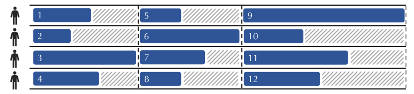
Figure 1. Synchronous mechanism in hyper-parameter tuning, where each row represents a worker. The deep-blue areas correspond to the evaluation process of configurations; the striped areas refer to idle time.

An Emerging Challenge in Scalability. This paper is inspired by our efforts applying these latest methods to applications running at a large Internet company. One critical challenge arises from the gap between the scalability of existing automatic tuning methods and the ever-growing complexity of industrial-scale models. In recent years, we have witnessed that evaluating ML models are getting increasingly expensive as the size of datasets and models grows larger. For example, it takes days to train NASNet (Zoph et al., 2018) to convergence on ImageNet, not to mention models like GPT-3 (Brown et al., 2020) with hundreds of billions of parameters. Unfortunately, it is difficult for existing tuning methods to scale well to such tasks with ever-increasing evaluation costs, thus leading to a sub-optimal configuration for deployment. When deploying existing approaches in large-scale applications, we realize some limitations in the following three aspects:

(1) Design of Partial Evaluations. Since the complete evaluation of a configuration is usually expensive (e.g., training deep learning models or training ML models on large-scale datasets), recent studies propose to evaluate configurations using partial resources (e.g., training models using a few epochs or a subset of the training set) (Jamieson and Talwalkar, 2016; Li et al., 2018a; Poloczek et al., 2017). However, how many training resources should be allocated to each partial evaluation? This question is non-trivial: (1) evaluations with small training resources could decrease evaluation cost, however, may be inaccurate to guide the search process; whereas (2) over-allocating resources could have the risk of high evaluation costs but diminishing returns from precision improvements. How can we automatically decide on the right level of resource allocation to balance the “precision vs. cost” trade-off in partial evaluations? This question remains open in state-of-the-arts (Falkner et al., 2018; Tiao et al., 2020; Li et al., 2021a).

(2) Utilization of Parallel Resources. Along with the rapid increase of evaluation cost, it comes with the rise of computation resources made available by industrial-scale clusters. However, state-of-the-arts, such as BOHB (Falkner et al., 2018) and MFES-HB (Li et al., 2021a), often use a synchronous architecture, which often cannot fully utilize all computation resources due to the synchronization barrier and are often sensitive to stragglers (See Figure 1). ASHA (Li et al., 2018b) is able to remove these issues associated with synchronous promotions by incurring a number of inaccurate promotions, while this asynchronous promotion could hamper the sample efficiency when utilizing the parallel and distributed resources. Thus, we need to explore an efficient asynchronous mechanism which pursues both sample efficiency and high utilization of parallel resources simultaneously.

(3) Support of Advanced Multi-fidelity Optimizers. While there are recent advancements in the design of Bayesian optimization methods, most, if not all, distributed tuning systems (Golovin et al., 2017; Falkner et al., 2018; Li et al., 2020a) have not fully utilized these advanced algorithms. For example, while there are algorithms that can more effectively exploit the low-fidelity measurements generated by partial evaluations (Li et al., 2021a), many existing systems (Feurer et al., 2015; Falkner et al., 2018) still depend on vanilla Bayesian optimization methods that only use the high-fidelity measurements from the complete evaluations. Can we design a flexible system architecture to conveniently support drop-in replacement of different optimizers under the async/synchronous parallel settings? This question is especially important from a system perspective.

Contributions. Inspired by our experience and observations deploying these state-of-the-art methods in our scenarios, in this paper, (C.1) we propose Hyper-Tune, an efficient distributed automatic hyper-parameter tuning framework. Hyper-Tune has three core components: resource allocator, evaluation scheduler, and generic optimizer, each of which corresponds to one aforementioned question: (1) To accommodate the first issue, we design a simple yet novel resource allocation method that could search for a good allocation via trial-and-error, and this method can automatically balance the trade-off between the precision and cost of evaluations. (2) To mitigate the second issue, we propose an efficient asynchronous mechanism – D-ASHA, a novel variant of ASHA (Li et al., 2020a). D-ASHA pursues the following two aspects simultaneously: (i) synchronization efficiency: the overhead of synchronization in wall-clock time, and (ii) sample efficiency: the number of runs that the algorithm needs to converge. (3) To tackle the third issue, we provide a modular design that allows us to plug in different hyper-parameter tuning optimizers. This flexible design allows us to plug in MFES-HB (Li et al., 2021a), a recently proposed multi-fidelity optimizer. In addition, we also adopt an algorithm-agnostic sampling framework, which enables each optimizer algorithm to adapt to the sync/asynchronous parallel scenarios easily. (C.2) We conduct extensive empirical evaluations on both publicly available benchmark datasets and a large-scale real-world dataset in production. Hyper-Tune achieves strong anytime and converged performance and outperforms state-of-the-art methods/systems on a wide range of hyper-parameter tuning scenarios: (1) XGBoost with nine hyper-parameters, (2) ResNet with six hyper-parameters, (3) LSTM with nine hyper-parameters, and (4) neural architectures with six hyper-parameters. Compared with the state-of-the-art BOHB (Falkner et al., 2018) and A-BOHB (Tiao et al., 2020), Hyper-Tune achieves up to $11.2\times$ and $5.1\times$ speedups, respectively. In addition, it improves the AUC by 0.87% in an industrial recommendation application with a billion instances.

Overview. This paper is organized as follows. We discuss the related work in Section 2. In Section 3, we review Bayesian optimization, synchronous Hyperband, as well as asynchronous ASHA. The proposed framework is presented in Section 4. We provide empirical evaluations for hyper-parameter tuning problems in Section 5 and end this with the conclusion and future work in Section 6.

2. Related Work

Bayesian optimization (BO) has been successfully applied to hyper-parameter tuning (Snoek et al., 2012; Bergstra et al., 2011; Hutter et al., 2011, 2019; Yao et al., 2018). Instead of using complete evaluations, Hyperband (Li et al., 2018a) (HB) dynamically allocates resources to a set of random configurations, and uses the successive halving algorithm (Jamieson and Talwalkar, 2016) to stop badly-performing configurations in advance. BOHB (Falkner et al., 2018) improves HB by replacing random sampling with BO. Two methods (Domhan et al., 2015; Klein et al., 2017c) propose to guide early-stopping via learning curve extrapolation. Vizier (Golovin et al., 2017), Ray Tune (Liaw et al., 2018) and OpenBox (Li et al., 2021b) also include a median stopping rule to stop the evaluations early. In addition, multi-fidelity methods (Klein et al., 2017a; Baker et al., 2017; Hu et al., 2019; Dai et al., 2019; Li et al., 2021a; Tiao et al., 2020) also exploit the low-fidelity measurements from partial evaluations to guide the search for the optimum of objective function $f$. MFES-HB (Li et al., 2021a) combines HB with multi-fidelity surrogate based BO.

Many methods (González et al., 2016; Azimi et al., 2010; Kandasamy et al., 2017b) can evaluate several configurations in parallel instead of sequentially. However, most of them (González et al., 2016), including BOHB (Falkner et al., 2018), focus on designing batches of configurations to evaluate at once, and few support asynchronous scheduling. ASHA (Li et al., 2018b) introduces an asynchronous evaluation paradigm based on successive halving algorithm (Jamieson and Talwalkar, 2016). In addition, Many approaches (Kandasamy et al., 2018a; Alvi et al., 2019) with asynchronous parallelization cannot exploit multiple fidelities of the objective; A-BOHB (Tiao et al., 2020) supports asynchronous multi-fidelity hyper-parameter tuning. Searching architecture hyper-parameters for neural networks is a popular tuning application. Recent empirical studies (Dong and Yang, 2019; Siems et al., 2020) show that sequential Bayesian optimization methods (Ma et al., 2019; White et al., 2019; Kandasamy et al., 2018b; Ru et al., 2020) achieve competitive performance among a number of NAS methods (Real et al., 2019; Liu et al., 2018; Awad et al., 2020; Xu et al., 2019; Zoph et al., 2018), which highlights the essence of parallelizing these BO related methods.

A-BOHB (Tiao et al., 2020) is the most related method compared with Hyper-Tune, while it suffers from the first issue. BOHB (Falkner et al., 2018) lacks design to tackle the aforementioned three problems, and MFES-HB (Li et al., 2021a) also faces these first and second issues. Instead, Hyper-Tune is designed to accommodate the three issues simultaneously.

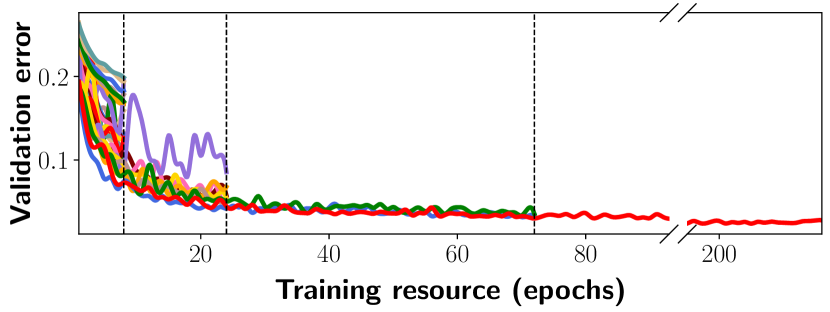
Figure 2. One iteration of successive halving algorithm (SHA) when tuning a CNN on MNIST, where $n_{1}=27$, $r_{1}=1$, $R=27$, $\eta=3$, and one unit of resource corresponds to 8 epochs. First, 27 configurations are evaluated with 1 unit of resource, i.e., 8 epochs ($n_{1}=27$ and $r_{1}=1$). Then the top $\eta^{-1}$ configurations continue their evaluations with $\eta$ times units of resources (i.e., $n_{2}=27*\eta^{-1}=9$ and $r_{2}=r_{1}*\eta=3$). Finally, only one configuration is evaluated with the maximum resource $R$.

3. Preliminary

We define the hyper-parameter tuning as a black-box optimization problem, where the objective value $f(\bm{x})$ (e.g., validation error) reflects the performance of an ML algorithm with given hyper-parameter configuration $\bm{x}\in\mathcal{X}$. The goal is to find the optimal configuration that minimizes the objective function $\bm{x}^{\ast}=\arg\min_{\bm{x}\in\mathcal{X}}f(\bm{x})$, and the only mode of interaction with $f$ is to evaluate the given configuration $\bm{x}$. In the following, we introduce existing methods for solving this black-box optimization problem, and these methods are the basic ingredients in Hyper-Tune.

3.1. Bayesian Optimization

The main idea of Bayesian optimization (BO) is as follows. Since evaluating the objective function $f$ for configuration $\bm{x}$ is very expensive, it approximates $f$ using a probabilistic surrogate model $M:p(f|D)$ that is much cheaper to evaluate. In the $n^{th}$ iteration, BO methods iterate the following three steps: (1) use the surrogate model $M$ to select a configuration that maximizes the acquisition function $\bm{x}_{n}=\arg\max_{\bm{x}\in\mathcal{X}}a(\bm{x};M)$, where the acquisition function is used to balance the exploration and exploitation; (2) evaluate the configuration $\bm{x}_{n}$ to get its performance $y_{n}$; (3) add this measurement $(\bm{x}_{n},y_{n})$ to the observed measurements $D=\{(\bm{x}_{1},y_{1}),...,(\bm{x}_{n-1},y_{n-1})\}$, and refit the surrogate $M$ on the augmented $D$. Popular acquisition functions include EI (Jones et al., 1998), PI (Snoek et al., 2012), UCB (Srinivas et al., 2010), etc. Due to the ever-increasing evaluation cost, several researches (Wang et al., 2013; Falkner et al., 2018) reveal that vanilla BO methods with complete evaluations fail to converge to the optimal configuration quickly.

3.2. Hyperband

To address the issue in vanilla BO methods, Hyperband (HB) (Li et al., 2018a) proposes to speed up configuration evaluations by early stopping the badly-performing configurations. It has the following two loops:

(1) Inner loop: successive halving. HB extends the original successive halving algorithm (SHA) (Jamieson and Talwalkar, 2016), which serves as a subroutine in HB, and here we also refer to it as SHA. SHA is designed to identify and terminate poor-performing hyper-parameter configurations early, instead of evaluating each configuration with complete training resources, thus accelerating configuration evaluation. Given a kind of training resource (e.g., the number of iterations, the size of training subset, etc.), SHA first evaluates $n_{1}$ hyper-parameter configurations with the initial $r_{1}$ units of resources each, and ranks them by the evaluation performance. Then it promotes the top $1/\eta$ configurations to continue its training with $\eta$ times larger resources (usually $\eta=3$), that’s, $n_{2}=n_{1}*\eta^{-1}$ and $r_{2}=r_{1}*\eta$, and stops the evaluations of the other configurations in advance. This process repeats until the maximum training resource $R$ is reached. Figure 2 gives a concrete example of SHA.

(2) Outer loop: the choice of $r_{1}$ and $n_{1}$. Given some finite budget $B$ for each bracket, the values of $r_{1}$ and $n_{1}=\frac{B}{r_{1}}$ should be carefully chosen because a small initial training resource $r_{1}$ with a large $n_{1}$ may lead to the elimination of good configurations in SHA iterations by mistake. There is no prior whether we should use a smaller initial training resource $r_{1}$ with a larger $n_{1}$, or a larger $r_{1}$ with a smaller $n_{1}$. HB addresses this problem by enumerating several feasible values of $r_{1}$ in the outer loop, where the inner loop corresponds to the execution of SHA. Table 1 shows a concrete example about the number of evaluations and their corresponding training resources in an iteration of HB, where each column corresponds to the results of inner loop (i.e., one iteration of SHA with different $r_{1}$s). For example, the first column “Bracket-1” of Table 1 corresponds to the execution process of SHA in Figure 2. Note that, the HB iteration will be called multiple times until the tuning budget exhausts.

Table 1. The values of $n_{i}$ and $r_{i}$ in the HB evaluations, where $R=27$ and $\eta=3$. Each column displays an inner loop (SHA process). The pair ($n_{i}$, $r_{i}$) in each cell means there are $n_{i}$ configuration evaluations with $r_{i}$ units of training resources. Taking the first column “Bracket-1” as an example, the evaluation process corresponds to the iteration of SHA in Figure 2. It starts with $n_{1}=27$ config evaluations with $r_{1}=1$ unit of resources; then the top $n_{2}=9$ evaluations continue with $r_{2}=3$; then $n_{3}=3$ and $r_{3}=9$; finally, only $n_{4}=1$ config gets the maximum resource $r_{4}=27$.

	Bracket-1			Bracket-2			Bracket-3			Bracket-4
$i$	$n_{i}$		$r_{i}$	$n_{i}$		$r_{i}$	$n_{i}$		$r_{i}$	$n_{i}$		$r_{i}$
$1$	$27$		$1$	$12$		$3$	$6$		$9$	$\bm{4}$		$27$
$2$	$9$		$3$	$4$		$9$	$\bm{2}$		$27$
$3$	$3$		$9$	$\bm{1}$		$27$
$4$	$\bm{1}$		$27$

Definitions. We refer to SHA with different initial training resources – $r_{1}$s as brackets (See Table 1), and the evaluations with certain units of training resources as resource level.

Partial Evaluation Design Issue in HB. Since HB-style methods (Li et al., 2018a; Falkner et al., 2018; Li et al., 2021a) own excellent features, such as flexibility, scalability, and ease of parallelization, we build our framework based on HB. HB consists of multiple brackets (i.e., SHA procedures), and each of them requires an $r_{1}$ as input. HB enumerates several feasible values of $r_{1}$, and executes each corresponding bracket sequentially and repeatedly. Bracket-$i$ is equipped with $r_{1}=\eta^{i-1}$ units of initial training resources, so each bracket corresponds to a kind of partial evaluation design. When digging deeper into the HB framework, we observe the “precision vs. cost” tradeoff caused by the selection of bracket (i.e., each kind of partial evaluation design) as follows: (1) The partial evaluation with a small $r_{1}$ implies that few training resources are allocated, and this may incur a larger number of inaccurate promotions in SHA, i.e., poor configurations are promoted to the next resource level, and good configurations are terminated by mistake due to the low fidelity. (2) As $r_{1}$ becomes large, the partial evaluation design has the risk of high evaluation cost but diminishing returns from precision improvements. While HB tries each bracket sequentially and repeatedly, it is inevitable that it wastes evaluation cost when applying a large number of inappropriate brackets during optimization. To develop an efficient tuning system, we need to revisit the HB pipeline and answer the following question: Can we automatically learn the right level of resource allocation (i.e., proper partial evaluation design) that balances the “precision vs. cost” tradeoff well? In Section 4.1 we describe our bracket selection based solution to this problem.

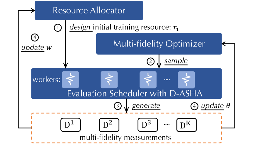
Figure 3. The framework of Hyper-Tune.

4. Proposed Framework

In this section, we first give the overview of the proposed framework, and then describe three core components that are designed to accommodate the aforementioned three issues in Section 1.

Framework Overview. The proposed framework – Hyper-Tune takes the tuning task and time budget as inputs, and outputs the best configuration found in the search process. Hyper-Tune has three components: resource allocator (Section 4.1), evaluation scheduler (Section 4.2), and multi-fidelity optimizer (Section 4.3). It is an iterative framework that will repeat until the given budget exhausts. Figure 3 illustrates an iteration of Hyper-Tune, with four concrete steps. The resource allocator selects the initial training resources $r_{1}$ when evaluating configurations (Step 1), which directly determines partial evaluation design. Then the multi-fidelity optimizer will sample a configuration from the search space for each idle worker (Step 2). The evaluation scheduler then evaluates these configurations with the corresponding training resources in parallel (Step 3). Finally, based on the multi-fidelity results from parallel evaluations, Hyper-Tune updates the parameters in resource allocator and multi-fidelity optimizer (Step 4), respectively.

Basic Setting: Measurements and Base Surrogates. Due to the flexibility and scalability of HyperBand (HB) (Li et al., 2018a, b; Falkner et al., 2018; Tiao et al., 2020), we build our framework on HB. Then we collect the results from evaluations with different resource levels, and we refer to them as “measurements”. According to the number of training resources used by the evaluations, we can categorize the measurements into $K$ groups: $D_{1},...,D_{K}$, where $K=\lfloor\log_{\eta}(R)\rfloor+1$, $\eta$ is the discard proportion in HB, $R$ is the maximum training resources for evaluation, and typically $K$ is less than $7$. The measurement ($\bm{x}$, $y$) in each group $D_{i}$ with $i\in[1:K]$ is obtained by evaluating configuration $\bm{x}$ with $r_{i}=\eta^{i-1}$ units of training resources. Thus $D_{K}$ denotes the high-fidelity measurements from the complete evaluations with the maximum training resources $r_{K}=R$, and $D_{1:K-1}$ denote the low-fidelity measurements from the partial evaluations. In Hyper-Tune, we build $K$ base surrogates: $M_{1:K}$, where surrogate $M_{i}$ is trained on the group of measurements $D_{i}$. In the following sections, we introduce the design of each component.

4.1. Resource Allocation with Bracket Selection

Challenge. The resource allocator aims to design the proper partial evaluations automatically. As stated in Section 3.2, the optimal bracket (i.e., the optimal initial training resources that balance the “precision vs. cost” trade-off well) minimizes the evaluation cost while keeping a high precision of partial evaluations. We need to automatically deal with this trade-off. The resource allocator needs to identify the optimal bracket in HB, where each bracket corresponds to a type of initial resource design for partial evaluation.

Solution Overview. We adopt the “trial-and-error” paradigm to identify the optimal bracket in an iterative manner. In each iteration, it iterates the following three steps: (1) we first select a bracket (i.e., partial evaluation design involving $n_{1}$ configurations with $r_{1}$ initial training resources) based on parameters $\bm{w}$; (2) once the $i^{th}$ bracket is chosen, we execute this bracket; (3) based on the measurements from these evaluations, we could update the parameters $\bm{w}$. For Step 1, in the beginning, we select brackets by round-robin with three times (as initialization); then we sample a bracket using parameters $\bm{w}$, where each $w_{i}$ with $i\in[1:K]$ indicates the probability of this bracket being the optimal one. For Step 3, we propose a two-stage technique to calculate $\bm{w}$ that balances the above trade-off. In the first stage, we learn a parameter $\theta_{i}$ for each bracket, where $\theta_{i}$ is proportional to the precision of evaluations with the training resources $r_{i}$. In the second stage, we multiply each $\theta_{i}$ with a coefficient $c_{i}$ to obtain the final $w_{i}$. This coefficient is inversely proportional to the training resources in the partial evaluation; in this way, the strategy tends to choose the bracket with small training resources. By the multiplication between $c_{i}$ and $\theta_{i}$ ($w_{i}=c_{i}\cdot\theta_{i}$), we could balance the “precision vs. cost” trade-off in partial evaluations.

To measure precision, we focus on the partial orderings of measurements among different resource levels. If configuration $\bm{x}_{1}$ performs better than $\bm{x}_{2}$ when the training resource is $r$, given the complete training resource $\bm{x}_{1}$ still outperforms $\bm{x}_{2}$, indicating that the partial evaluations with $r$ units of training resources are accurate, so we can utilize this to measure the precision of evaluations. To implement this, we utilize the predictions of base surrogate $M_{i}$ built on $D_{i}$, and compare the predictive rankings of configurations with the rankings in $D_{K}$. For base surrogates $M_{1:K-1}$, we define the ranking loss as the number of miss-ranked pairs as follows:

(1) $$\scriptsize\mathbb{L}(M_{i})=\sum_{j=1}^{N_{K}}\sum_{k=1}^{N_{K}}\mathds{1}((M_{i}(\bm{x}_{j})<M_{i}(\bm{x}_{k})\otimes(y_{j}<y_{k})),$$

where $\otimes$ is the exclusive-or operator, $N_{K}=|D_{K}|$, and $(\bm{x_{i}},y_{i})$ is the measurement in $D_{K}$. For the base surrogate $M_{K}$ trained on $D_{K}$ directly, we adopt 5-fold cross-validation to calculate its $\mathbb{L}(M_{K})$. Further we define each $\theta_{i}$ as the probability that base surrogate $M_{i}$ has the least ranking loss. Concretely, we use Markov chain Monte Carlo (MCMC) to learn $\bm{\theta}$ by drawing $S$ samples: $l_{i,s}\sim\mathbb{L}(M_{i})$ for $s=1,...,S$ and each surrogate $i=1,...,K$, and calculating

(2) $$\scriptsize\theta_{i}=\frac{1}{S}\sum_{s=1}^{S}\mathds{1}\left(i=\mathop{\arg\min}_{i^{\prime}}l_{i^{\prime},s}\right).$$

To obtain $\bm{c}$, in Hyper-Tune we simply apply the inverse of the corresponding training resources, i.e., $c_{i}=1/r_{i}$. Finally, we normalize the raw $\bm{w}=\bm{c}\circ\bm{\theta}$ to obtain the final $\bm{w}$, where $\sum_{i}{w_{i}}=1$.

4.2. Asynchronous Evaluation Scheduling

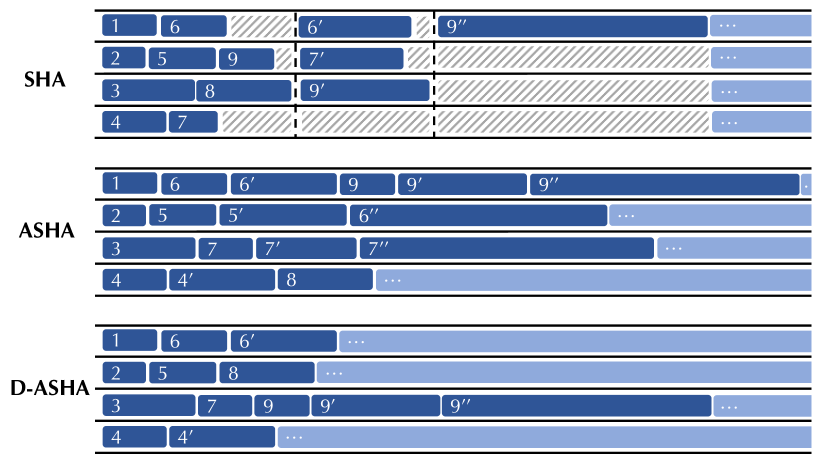
Figure 4. Three scheduling mechanisms on a real-world case, where each row corresponds to a worker, and the ranking of configurations are $\bm{x}_{3}$, $\bm{x}_{8}$, $\bm{x}_{2}$, $\bm{x}_{1}$, $\bm{x}_{4}$, $\bm{x}_{5}$, $\bm{x}_{6}$, $\bm{x}_{7}$, $\bm{x}_{9}$ (latter is the better). $i$’ refers to promoted evaluation of configuration $\bm{x}_{i}$. Each deep-blue block with $i$ corresponds to the evaluation process of $\bm{x}_{i}$; the light-blue blocks represent the evaluations for other iterations of SHA procedures; the striped areas in SHA refer to no evaluations for workers.

Challenge. In this section, we introduce the distributed scheduling mechanism in the evaluation scheduler. SHA (Jamieson and Talwalkar, 2016) promotes the top $1/\eta$ configurations to the next resource level until all configurations in the current level have been evaluated (synchronization barrier). Due to the synchronous design, which often leads to the straggler issue, the ineffective use of computing resources in SHA is inevitable. ASHA (Li et al., 2020a) is able to remove these issues associated with synchronous promotions by incurring a number of inaccurate promotions (See Figure 4), i.e., configurations that fall into the top $1/\eta$ early but are not in the actual top $1/\eta$ of all configurations. However, this frequent and inaccurate promotion could hamper the sample efficiency when utilizing the parallel and distributed resources, i.e., ASHA may spend lots of training resources on evaluating the less promising configurations. Therefore, we need an efficient scheduling method which pursues high sample efficiency while keeping the advantage of asynchronous mechanism.

Input: initial training resource $r_{1}$, maximum resource $R$, discard proportion $\eta$.

1

2Function $\operatorname{D-ASHA()}$:

3   $\bm{x},r_{x}=\operatorname{get\_job()}$;

4   Assign a job with configuration $\bm{x}$ and resource $r_{x}$ to a free worker.

5Function $\operatorname{get\_job()}$:

6   // Check if we need to promote configurations.

7  for $k=\lfloor log_{\eta}(R)\rfloor,...,2,1$, do

8     // $D_{k}$ refers to measurements of resource level $k$.

9     Configuration candidates $\mathit{C}=\{{\bm{x}}\ \text{for}\ {\bm{x}}\in$ top $1/\eta$ configurations in $D_{k}$ if $\bm{x}$ has not been promoted}

10    if $|D_{k}|/(|D_{k+1}|+1)\geq\eta$ and $|\mathit{C}|>0$, then

11      return $\mathit{C}[0],\eta^{k}$

12    end if

13  end for

14  Sample a configuration $\bm{x}$ based on the multi-fidelity optimizer.

  return $\bm{x},r_{1}$

Algorithm 1 Pseudo Code for D-ASHA.

Delayed ASHA. To alleviate this issue, we propose a variant of ASHA — delayed ASHA (abbr. D-ASHA), which uses a delay strategy to decrease inaccurate promotions and still preserves the asynchronous scheduling mechanism. Instead of promoting each configuration that is in the top $1/\eta$ of all previously-evaluated configurations, D-ASHA promotes configurations to the next level if (1) the configuration is in the top $1/\eta$ of configurations, and (2) the number of collected measurements $|D_{k}|$ with current resource level should be $\eta$ times larger than the number of the next level’s $|D_{k+1}|$ if promoted (Lines 9-10 in Algorithm 1). The inaccurate promotions (in Cond.1) arise from a small number of observed measurements in $D_{k}$ with current resource level. The condition 2 ensures that $|D_{k}|$ should be larger than a threshold $\eta|D_{k+1}|$, i.e., $|D_{k}|/(|D_{k+1}|+1)\geq\eta$. In this way, the delay strategy could prevent the frequent promotion issue in ASHA, and further improve the sample efficiency. Figure 4 gives a concrete real-world example to explain this design. Algorithm 1 provides the formulated description about D-ASHA. Additionally, if no promotions are possible, D-ASHA requests a new configuration from the multi-fidelity optimizer (provided in Algorithm 2) and adds it to the base level (Lines 13-14), so that more configurations can be promoted to the upper levels.

4.3. Multi-fidelity Configuration Sampling

Challenge. There are various advancements in the design of Bayesian optimization (BO) methods. While those algorithms differ in the execution process, a flexible tuning system should contain an optimizer module that allows us to plug in different hyper-parameter tuning optimizers easily. In addition, since most BO based methods are intrinsically sequential, it is impractical to modify each possible algorithm to support parallel scenarios case by case. Thus, we need an algorithm-agnostic framework to extend different sequential optimizers to support parallel evaluations in both sync/asynchronous settings.

Optimizer Design. To tackle the first challenge, we provide a generic optimizer abstraction for configuration sampling in Hyper-Tune. It includes 1) the data structure to store multi-fidelity measurements: $D_{1}$, …, $D_{K}$, and 2) the fit and predict APIs for surrogate model. This abstraction enables convenient support/implementation of different configuration sampling algorithms (e.g., random search, Bayesian optimization, multi-fidelity optimization, etc.). For the second challenge, we further propose an algorithm-agnostic sampling framework to support asynchronous and synchronous parallel evaluations conveniently without any ad-hoc modifications.

(Multi-fidelity Optimizer.) Multi-fidelity methods (Klein et al., 2017b; Kandasamy et al., 2017a; Poloczek et al., 2017; Hu et al., 2019; Sen et al., 2018; Wu et al., 2019; Li et al., 2020b) have achieved success in hyper-parameter tuning. Meanwhile, it produces multi-fidelity measurements which can help determine the optimal bracket for evaluation. In Hyper-Tune, we implement a multi-fidelity optimizer by default based on MFES-HB (Li et al., 2020b) to utilize multi-fidelity measurements, and build a multi-fidelity ensemble surrogate by combining all base surrogates:

$$M_{\text{MF}}=\texttt{agg}(\{M_{1},...,M_{K}\};{\bm{\theta}});$$

The surrogate $M_{\text{MF}}$ is used to guide the configuration search, instead of the high-fidelity surrogate $M_{K}$ only, in the framework of BO. Concretely, we combine the base surrogates with weighted bagging, and the weights $\bm{\theta}$ are exactly the parameters obtained in Section 4.1. Each $\theta_{i}$ also reflects the reliability when applying the corresponding low-fidelity information from partial evaluations with $r_{i}$ units of training resources to the target problem. Finally, the predictive mean and variance of $M_{MF}$ at configuration $\bm{x}$ are given by:

(3) $$\mu_{MF}(\bm{x})=\sum_{i}\theta_{i}\mu_{i}(\bm{x}),\quad\sigma_{MF}^{2}(\bm{x})=\sum_{i}\theta_{i}^{2}\sigma_{i}^{2}(\bm{x}),$$

where $\mu_{i}(\bm{x})$ and $\sigma_{i}^{2}(\bm{x})$ are the mean and variance predicted by the base surrogate $M_{i}$ at configuration $\bm{x}$. Based on the multi-fidelity measurements, this multi-fidelity surrogate could learn the objective function well, and can be used to speed up the search process.

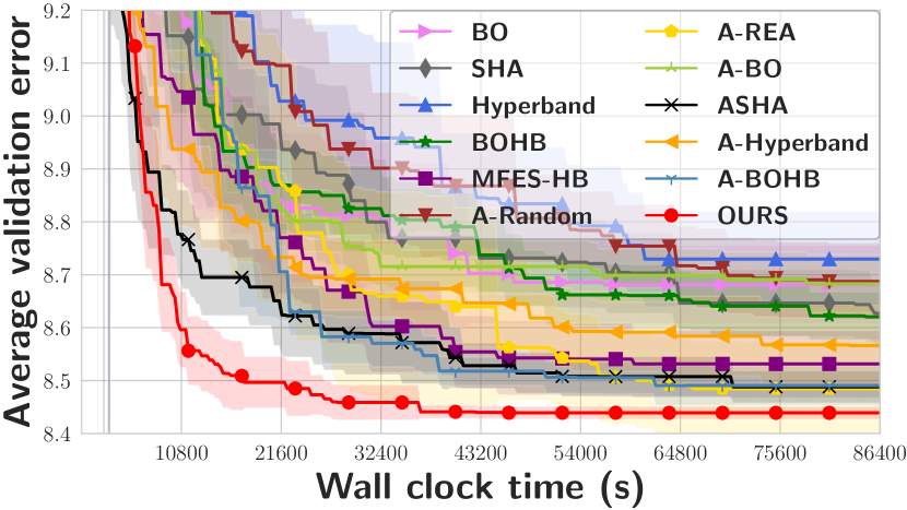
(a) CIFAR-10-valid

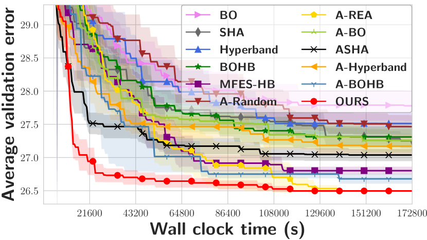
(b) CIFAR-100

(c) ImageNet16-120

Figure 5. Validation error (%) of tuning architectures on three datasets based on NAS-Bench-201.

(Algorithm-agnostic Sampling.) Since traditional BO methods are intrinsically sequential, we need an algorithm-agnostic framework to extend the sequential method to the sync/asynchronous parallel settings seamlessly, and meanwhile ensure convergence. In parallel evaluations, each worker pulls a new configuration to evaluate after the previous evaluation is completed; there are pending evaluations that are not finished when sampling new configurations. We need to sample new configurations that are promising and far enough from the configurations being evaluated by other workers to avoid repeated or similar evaluations. To this end, we adopt an algorithm-agnostic sampling framework, which leverages the local penalization-based strategy (González et al., 2016; Li et al., 2021b) to deal with the above issue, where each pending evaluation is imputed with the median of performance in $D_{K}$. This framework enables that each algorithm could adapt to the parallel scenarios easily. Algorithm 2 gives the algorithm-agnostic sampling procedure of optimizers.

Input: the hyper-parameter space $\mathcal{X}$, measurements $D_{1}$, $D_{2}$, …, $D_{K}$, pending configurations $C_{\text{pending}}$ being evaluated on workers, the multi-fidelity surrogate $M_{MF}$, and acquisition function $\alpha(\cdot)$.

1 calculate $\hat{y}$, the median of $\{y_{i}\}_{i=1}^{n}$ in $D_{K}$;

2 impute new measurements $D_{\text{new}}=\{(\bm{x}_{\text{pending}},\hat{y}):\bm{x}_{\text{pending}}\in C_{\text{pending}}\}$;

3 refit the surrogate $M_{K}$ in $M_{MF}$ on $D_{\text{aug}}$, where $D_{\text{aug}}=D_{K}\cup D_{\text{new}}$, and build the acquisition function $\alpha(\bm{x},M)$ using $M_{MF}$;

return the configuration $\bm{x}^{\ast}=\operatorname{argmax}_{\bm{x}\in\mathcal{X}}\alpha(\bm{x},M_{MF})$.

Algorithm 2 Sampling procedure.

5. Experiments and Results

We now present empirical evaluations of Hyper-Tune. We first focus on the end-to-end efficiency between Hyper-Tune and other state-of-the-art systems. We then study two more specific aspects, with the following two hypotheses: Hyper-Tune is more robust to the low-fidelity measurements with different scales of noises (Robustness); Hyper-Tune can scale well to the scenarios with different evaluation cost and number of evaluation workers (Scalability).

5.1. Experimental Settings

Compared Methods.   We compare Hyper-Tune with the manual setting given by our enterprise partner and the following ten baselines. (1) A-Random: Asynchronous Random Search (Bergstra and Bengio, 2012) that selects random configurations to evaluate asynchronously, (2) BO: Batch-BO (González et al., 2016) that samples a batch of configurations to evaluate synchronously, (3) A-BO: Async Batch-BO (Li et al., 2021b) that samples a batch of configurations to evaluate asynchronously, (4) SHA: Successive Halving Algorithm (Jamieson and Talwalkar, 2016) that adaptively allocates training resources to configurations with multi-stage early-stopping, (5) ASHA (Li et al., 2020a) that improves SHA asynchronously via configuration promotion, (6) Hyperband (Li et al., 2018a) that applies a bandit strategy to allocate resources dynamically based on SHA, (7) A-Hyperband (Li et al., 2020a) that extends Hyperband to asynchronous settings via ASHA, (8) BOHB (Falkner et al., 2018) that combines the benefits of both Hyperband and Bayesian optimization, (9) A-BOHB (Tiao et al., 2020) that improves BOHB with asynchronous multi-fidelity optimizations, (10) MFES-HB (Li et al., 2021a) that combines Hyperband and multi-fidelity Bayesian optimization. Note that Batch-BO, SHA, Hyperband, BOHB, and MFES-HB are synchronous methods, and the others are asynchronous ones.

Tasks.   We run experiments on the following tuning tasks:

(1) Neural Architecture Search. We use the NAS-Bench-201 (Dong and Yang, 2019) which includes offline evaluations of neural network architectures. The search space consists of 6 hyper-parameters. The minimum and maximum number of epochs in NAS-Bench-201 are 1 and 200. HB-based methods use 4 brackets, and the default number of workers is 8. We evaluate Hyper-Tune on three built-in datasets – CIFAR-10-Valid, CIFAR-100, and ImageNet16-120, where the total budgets are 24, 48, and 120 hours, respectively. We finish each method once the simulated training time reaches the given budget.

(2) Tabular Classification. We tune XGBoost (Chen and Guestrin, 2016) on four large datasets from OpenML (Vanschoren et al., 2014) – Pokerhand, Covertype, Hepmass, and Higgs. The hyper-parameter space of XGBoost includes $9$ hyperparameters. For partial evaluations, we use the subset of the training set instead of using the entire set. The minimum and maximum size of subset are $1/27$ and $1$. HB-based methods use $4$ brackets, and the default number of workers is $8$. The time budgets for the above four datasets are $2$, $3$, $6$, and $6$ hours, respectively. Each worker is equipped with $8$ CPU cores during evaluation.

(3) Image Classification. We tune ResNet (He et al., 2016) on the image classification dataset – CIFAR-10. The search space includes batch size, SGD learning rate, SGD momentum, learning rate decay, and weight decay. Cropping and horizontal flips are used as default augmentation operations. The minimum and maximum number of epochs are 1 and 200. HB-based methods use 4 brackets, and the default number of workers is 4. The time budget is 48 hours. Each worker has 8 CPU cores and 1 GPU during evaluation.

(a) Pokerhand

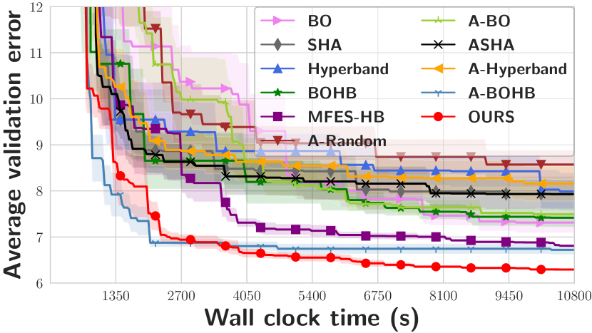
(b) Covertype

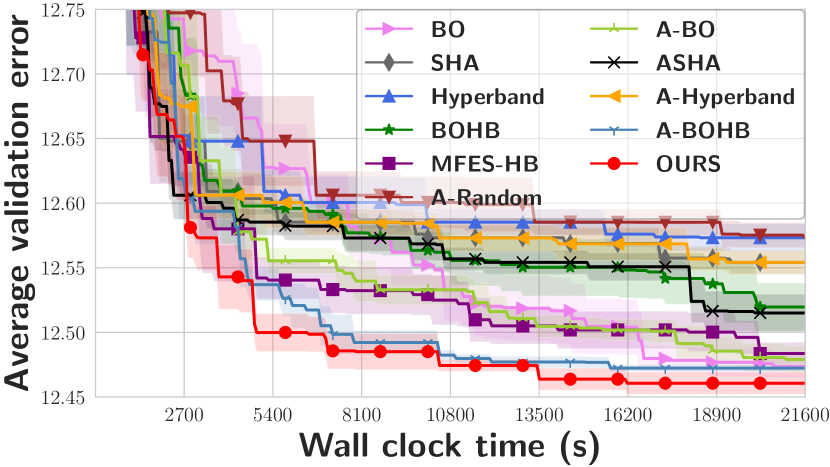
(c) Hepmass

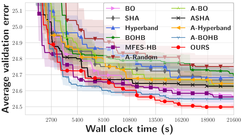
(d) Higgs

Figure 6. Validation error (%) of tuning XGBoost on four large datasets.

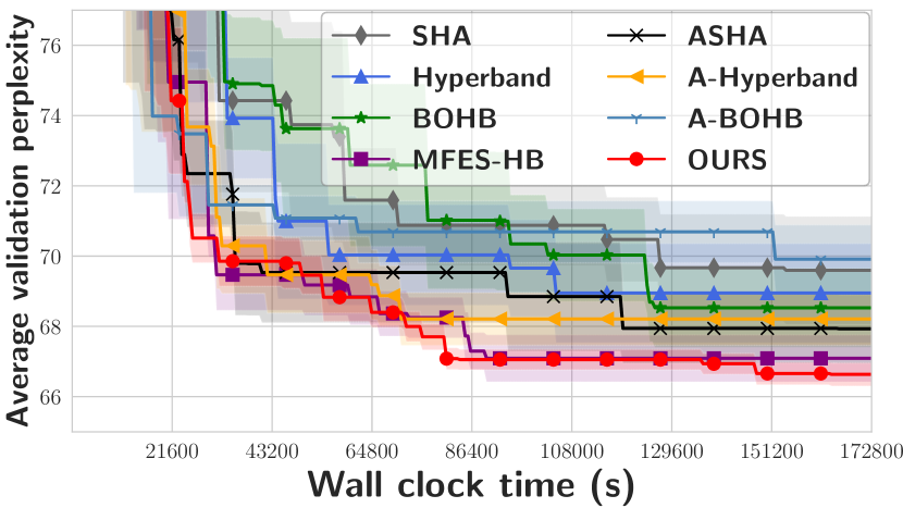
(a) LSTM on Penn Treebank

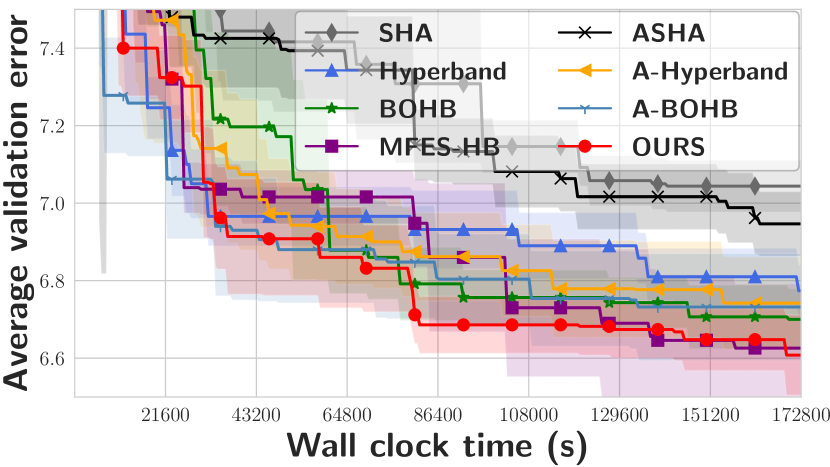
(b) ResNet on CIFAR-10

Figure 7. Results of tuning LSTM and ResNet.

(4) Language Modelling. We tune a 3-layer LSTM (Hochreiter and Schmidhuber, 1997) on the dataset Penn Treebank. The search space includes batch size, hidden size, learning rate, weight decay and five hyper-parameters related to dropout. The embedding size is 400. The minimum and maximum number of epochs are 1 and 200. HB-based methods use 4 brackets, and the time budget is 48 hours; the default number of workers is 4, and each worker uses 8 CPU cores and 1 GPU during evaluation.

Implementation Details.   Two metrics are used in our experiments, including (1) the classification error for XGBoost tuning, ResNet tuning, and neural architecture search, and (2) the perplexity when tuning LSTM. We use the validation and test performance stored in NAS-Bench-201 directly for neural architecture search. In the XGBoost tuning experiment, we randomly divide 60% of the total dataset as the training set, 20% as the validation set, and the left as the test set. In the other experiments, we split 20% of the training dataset as the validation set. Then, we track the wall clock time (including optimization overhead and evaluation cost), and store the lowest validation performance after each evaluation. The best configurations are then applied to the test dataset to report the test performance. All methods are repeated ten times with different random seeds, and the mean validation performance across runs is plotted. We include more experimental setups and reproduction details about Hyper-Tune in the supplementary material.

5.2. Architecture Search on NAS-Bench-201

Figure 5 shows the results on NAS-Bench-201 datasets. Due to the utilization of parallel resources issue in Hyperband, asynchronous random search (A-Random) outperforms synchronous Hyperband. Hyper-Tune obtains the best anytime and converged performance among all methods. Concretely, it achieves 8.2$\times$, 11.2$\times$ and 6.3$\times$ speedups against BOHB, and obtains 3.3$\times$, 2.9$\times$, and 2.0$\times$ speedups compared with A-BOHB on CIFAR-10-valid, CIFAR-100, and ImageNet16-120 respectively, which indicates its superior efficiency over the state-of-the-art methods. In addition, Hyper-Tune also gets the best test accuracy (See the results in Appendix A.5).

As reported in NAS-Bench-201 (Dong and Yang, 2019), the best method is regularized evolutionary algorithm (REA) (Real et al., 2019). For fair comparison, we also extend REA to an asynchronous version – A-REA. From Figure 5, we have that Hyper-Tune shows consistent superiority over A-REA. Remarkably, Hyper-Tune reaches the global optimum on CIFAR-100 and ImageNet-16-120 across all the ten runs, which also indicates the efficiency of Hyper-Tune.

Table 2. Test performance on three benchmarks. (accuracy (%) for XGBoost and ResNet, and perplexity for LSTM)

Method	XGBoost				ResNet	LSTM
	Covertype	Pokerhand	Hepmass	Higgs	CIFAR-10	Penn Treebank
Manual	86.91 $\pm$ 0.00	99.36 $\pm$ 0.00	87.06 $\pm$ 0.00	74.24 $\pm$ 0.00	91.88 $\pm$ 0.00	107.02 $\pm$ 0.00
BO	93.08 $\pm$ 0.19	99.32 $\pm$ 0.13	87.48 $\pm$ 0.01	75.40 $\pm$ 0.06	/	/
SHA	92.39 $\pm$ 0.40	98.43 $\pm$ 0.41	87.41 $\pm$ 0.02	75.30 $\pm$ 0.04	92.19 $\pm$ 0.30	66.05 $\pm$ 2.43
Hyperband	92.45 $\pm$ 0.37	98.30 $\pm$ 0.51	87.39 $\pm$ 0.02	75.29 $\pm$ 0.06	92.17 $\pm$ 0.31	65.93 $\pm$ 2.61
BOHB	92.97 $\pm$ 0.20	99.46 $\pm$ 0.07	87.44 $\pm$ 0.02	75.29 $\pm$ 0.05	92.37 $\pm$ 0.29	65.90 $\pm$ 2.15
MFES-HB	93.42 $\pm$ 0.08	99.61 $\pm$ 0.13	87.48 $\pm$ 0.01	75.44 $\pm$ 0.02	92.41 $\pm$ 0.24	64.21 $\pm$ 1.09
A-Random	91.99 $\pm$ 0.31	97.62 $\pm$ 0.53	87.38 $\pm$ 0.02	75.24 $\pm$ 0.07	/	/
A-BO	92.96 $\pm$ 0.09	99.47 $\pm$ 0.15	87.48 $\pm$ 0.01	75.35 $\pm$ 0.04	/	/
ASHA	92.61 $\pm$ 0.35	98.80 $\pm$ 0.24	87.46 $\pm$ 0.02	75.33 $\pm$ 0.05	92.23 $\pm$ 0.42	64.18 $\pm$ 0.58
A-Hyperband	92.39 $\pm$ 0.42	98.24 $\pm$ 0.46	87.41 $\pm$ 0.02	75.30 $\pm$ 0.04	92.16 $\pm$ 0.19	65.16 $\pm$ 1.22
A-BOHB	93.72 $\pm$ 0.10	99.83 $\pm$ 0.07	87.49 $\pm$ 0.01	75.49 $\pm$ 0.02	92.31 $\pm$ 0.25	66.02 $\pm$ 1.32
Hyper-Tune	93.97 $\pm$ 0.06	99.93 $\pm$ 0.03	87.52 $\pm$ 0.02	75.53 $\pm$ 0.03	92.48 $\pm$ 0.17	63.54 $\pm$ 0.38

5.3. Tuning XGBoost on Large Datasets

In Figure 6 and Table 2, we compare Hyper-Tune with the manual setting and ten competitive baselines by tuning XGBoost on four large datasets. The configurations from tuning algorithms outperform the manual settings on test results, which shows the necessity of tuning hyper-parameters for machine learning models. Different from the other experiments, the resource type here is the subset of dataset, i.e., we use different sizes of datasets subset to perform partial evaluation if necessary. As BO and A-BO evaluate each configuration completely, it takes them a long time to converge to a satisfactory performance due to expensive evaluation cost (15 minutes per trial on Covertype). In addition, Hyper-Tune and MFES-HB perform better than HyperBand, BOHB and most asynchronous methods, which indicates the advantage of leveraging low-fidelity measurements. Among the considered methods, Hyper-Tune achieves very competitive anytime performance, and obtains the best converged performance on all of the four datasets.

5.4. Tuning LSTM and ResNet

Figure 7(a) and Table 2 show the results of tuning LSTM on Penn Treebank. A-BOHB shows the worst converged performance among baselines, which we attribute to its failure of exploiting multi-fidelity measurements. A-Hyperband, MFES-HB, and Hyper-Tune show similar results in the early stage (19 hours), but after that, the perplexity of A-Hyperband stops decreasing as random sampling fails to exploit history observations efficiently. After 150k secs (about 41 hours), Hyper-Tune outperforms all baselines.

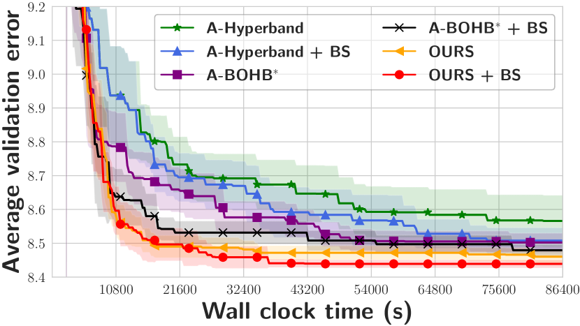
(a) NAS-Bench-201 on CIFAR-10-valid

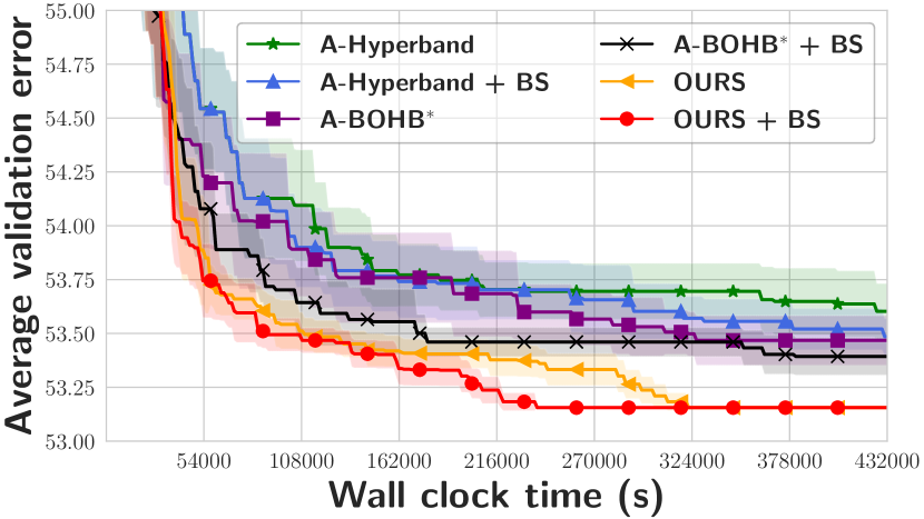
(b) NAS-Bench-201 on ImageNet16-120

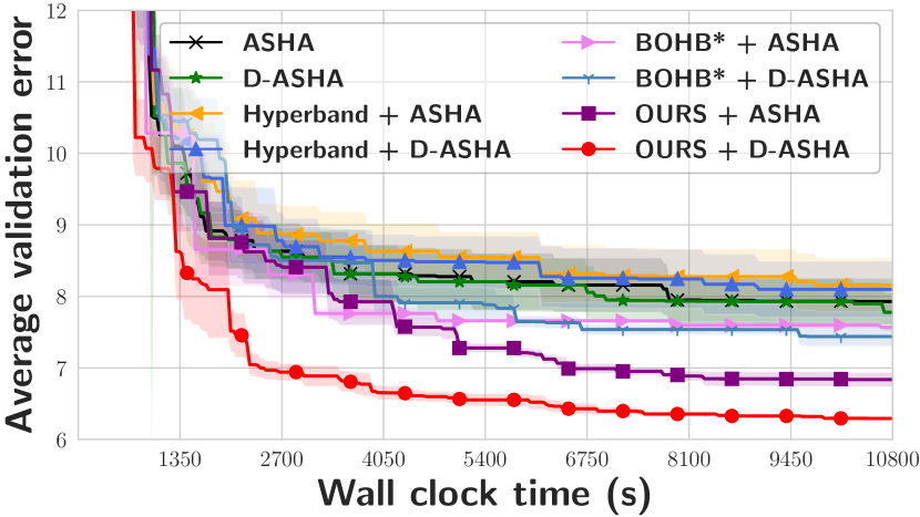
(c) XGBoost on Covertype

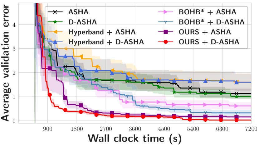
(d) XGBoost on Pokerhand

Figure 8. Ablation studies for different components in Hyper-Tune.

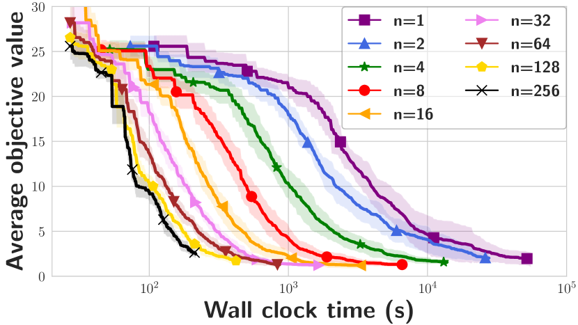
(a) Counting-ones Benchmark

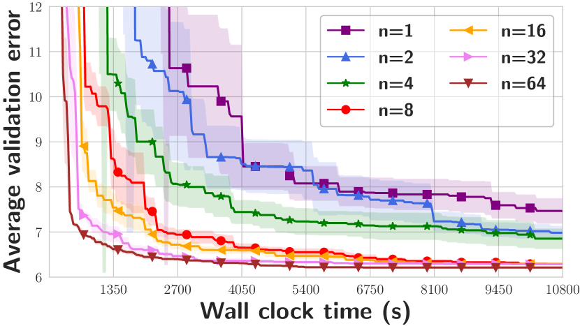
(b) XGBoost on Covertype

Figure 9. Scalability on the number of workers.

In Figure 7(b), we display the average error of tuning ResNet on CIFAR-10. As SHA and ASHA always start evaluating each configuration from the least resources, they cannot distinguish noisy low-fidelity results, which may explain their overall worst performance. Though Hyper-Tune and MFES-HB obtain a similar result (93.4%), Hyper-Tune shows a better anytime performance due to its asynchronous scheduling. Table 2 shows the test result.

5.5. Scalability Analysis

Figure 9 demonstrates the optimization curve with different number of parallel workers on two tuning tasks. We evaluate Hyper-Tune by tuning the counting-ones function  (Falkner et al., 2018) and XGBoost on Covertype. The details about the counting-ones function are provided in Appendix A.4. To demonstrate the scalablility of Hyper-Tune, we set the maximum number of workers to 256 and 64. On both tasks, the anytime performance is better when Hyper-Tune uses more workers, which indicates that Hyper-Tune scales to the number of workers well. Notably, Hyper-Tune with the maximum number of workers achieves 145.7x and 18.0x speedups compared with sequential Hyper-Tune on Counting-ones Benchmark and Covertype.

5.6. Industrial-Scale Tuning Application

In addition, we also evaluate Hyper-Tune on an industrial-scale tuning task for recommendation, which aims at identifying active users. The dataset provided by our enterprise partner includes more than one billion instances, and we train the model using the data of seven days and evaluate it using the data of the following day. The number of workers is 10 and the time budget is 48 hours. We evaluate ASHA, BOHB, A-BOHB and Hyper-Tune, and they improve the manual setting by -0.05%, 0.19%, 0.35% and 0.87%, respectively. Moreover, we conduct an ablation study on Hyper-Tune by keeping out one of the component in Table 3. We observe performance gain by introducing each component into Hyper-Tune while Bracket Selection leads to the largest gain. While at least one component is absent in competitive baselines, Hyper-Tune improves the AUC of the second-best baseline A-BOHB by 0.54%, which is a wide margin considering the potential commercial values.

5.7. Ablation Study

Effectiveness of Bracket Selection. Figure 8(a) and  8(b) illustrate the effectiveness of the proposed bracket selection method. We also add bracket selection (BS) to the asynchronous variant of Hyperband and BOHB. Note that the asynchronous BOHB here is parallelized via ASHA, but not A-BOHB mentioned in the experimental setups. We have that adding bracket selection helps asynchronous Hyperband, BOHB, and Hyper-Tune converge better. In addition, in Figure 8(b), though the converged performance of Hyper-Tune remains almost the same when bracket selection is employed, the anytime performance improves before 324k secs (90 hours). We owe this gain to the resource allocation strategy learned during optimization rather than attempting all the choices via round robin. In this way, as few as possible training resources are automatically allocated to evaluate the configurations, and this could effectively avoid evaluating poor configurations with too many resources.

Table 3. Ablation study on Hyper-Tune. The improvement indicates the performance gain upon manual settings.

Methods	Improvement (%)	$\Delta$ (%)
w/o BS	0.54	-0.33
w/o D-ASHA	0.75	-0.12
w/o MFES	0.56	-0.31
Hyper-Tune	0.87	-

Effectiveness of D-ASHA. Figure 8(c) and  8(d) show the results of applying D-ASHA to different methods. For ASHA, Hyperband and BOHB, we observe a slight improvement on both anytime and converged performance when applying D-ASHA. For Hyper-Tune, the validation error decreases by a large margin (0.5%) on Covertype with the aid of D-ASHA. The delay strategy could prevent the frequent promotion issue in ASHA, and further improve the sample efficiency. Therefore, D-ASHA could achieve a higher sample efficiency while keeping the advantage of asynchronous mechanism.

Effectiveness of Multi-fidelity Optimizer. We compare different optimizer for configuration sampling, including random sampling (A-Hyperband + BS), high-fidelity optimizer (A-BOHB + BS), and multi-fidelity optimizer (OURS + BS). As shown in Figure 8(a) and  8(b), we have that surrogate-based methods outperform random sampling, while multi-fidelity optimizer outperforms high-fidelity optimizer. The reason is that it takes the low-fidelity measurements into consideration when selecting the next configuration to evaluate. It also indicates that when performing hyper-parameter tuning, the low-fidelity measurements could provide useful information about the objective function, and can be used to speed up the search process.

6. Conclusion

In this paper, we presented Hyper-Tune, an efficient and robust distributed hyper-parameter tuning framework at scale. Hyper-Tune introduces three core components targeting at addressing the challenge in the large-scale hyper-parameter tuning tasks, including (1) automatic resource allocation, (2) asynchronous scheduling, and (3) multi-fidelity optimizer. The empirical results demonstrate that Hyper-Tune shows strong robustness and scalability, and outperforms state-of-the-art methods, e.g., BOHB and A-BOHB, on a wide range of tuning tasks.

References

- (1)
- Alvi et al. (2019) Ahsan Alvi, Binxin Ru, Jan-Peter Calliess, Stephen Roberts, and Michael A Osborne. 2019. Asynchronous Batch Bayesian Optimisation with Improved Local Penalisation. In International Conference on Machine Learning. PMLR, 253–262.
- Awad et al. (2020) Noor Awad, Neeratyoy Mallik, and Frank Hutter. 2020. Differential Evolution for Neural Architecture Search. arXiv preprint arXiv:2012.06400 (2020).
- Azimi et al. (2010) Javad Azimi, Alan Fern, and Xiaoli Z Fern. 2010. Batch bayesian optimization via simulation matching. In Advances in Neural Information Processing Systems. 109–117.
- Baker et al. (2017) Bowen Baker, Otkrist Gupta, Ramesh Raskar, and Nikhil Naik. 2017. Practical neural network performance prediction for early stopping. arXiv preprint arXiv:1705.10823 2, 3 (2017), 6.
- Baylor et al. (2017) Denis Baylor, Eric Breck, Heng-Tze Cheng, Noah Fiedel, Chuan Yu Foo, Zakaria Haque, Salem Haykal, Mustafa Ispir, Vihan Jain, Levent Koc, et al. 2017. Tfx: A tensorflow-based production-scale machine learning platform. In Proceedings of the 23rd ACM SIGKDD International Conference on Knowledge Discovery and Data Mining. 1387–1395.
- Bergstra and Bengio (2012) James Bergstra and Yoshua Bengio. 2012. Random search for hyper-parameter optimization. Journal of Machine Learning Research 13, Feb (2012), 281–305.
- Bergstra et al. (2011) James S Bergstra, Rémi Bardenet, Yoshua Bengio, and Balázs Kégl. 2011. Algorithms for hyper-parameter optimization. In Advances in neural information processing systems. 2546–2554.
- Boehm et al. (2020) Matthias Boehm, Iulian Antonov, Sebastian Baunsgaard, Mark Dokter, Robert Erich Ginthoer, Kevin Innerebner, Florijan Klezin, Stefanie Lindstaedt, Arnab Phani, Benjamin Rath, et al. 2020. SystemDS: A Declarative Machine Learning System for the End-to-End Data Science Lifecycle. In Conference on Innovative Data Systems Research.
- Breck et al. (2019) Eric Breck, Neoklis Polyzotis, Sudip Roy, Steven Euijong Whang, and Martin Zinkevich. 2019. Data Validation for Machine Learning. In 3rd Conference on Machine Learning and Systems (MLSys).
- Brown et al. (2020) Tom B Brown, Benjamin Mann, Nick Ryder, Melanie Subbiah, Jared Kaplan, Prafulla Dhariwal, Arvind Neelakantan, Pranav Shyam, Girish Sastry, Amanda Askell, et al. 2020. Language models are few-shot learners. arXiv preprint arXiv:2005.14165 (2020).
- Chen and Guestrin (2016) Tianqi Chen and Carlos Guestrin. 2016. Xgboost: A scalable tree boosting system. In Proceedings of the 22nd ACM SIGKDD International Conference on Knowledge Discovery and Data Mining. ACM, 785–794.
- Dai et al. (2019) Zhongxiang Dai, Haibin Yu, Bryan Kian Hsiang Low, and Patrick Jaillet. 2019. Bayesian Optimization Meets Bayesian Optimal Stopping. (2019), 1496–1506.
- Domhan et al. (2015) Tobias Domhan, Jost Tobias Springenberg, and Frank Hutter. 2015. Speeding Up Automatic Hyperparameter Optimization of Deep Neural Networks by Extrapolation of Learning Curves.. In IJCAI, Vol. 15. 3460–8.
- Dong and Yang (2019) Xuanyi Dong and Yi Yang. 2019. NAS-Bench-201: Extending the Scope of Reproducible Neural Architecture Search. In International Conference on Learning Representations.
- Falkner et al. (2018) Stefan Falkner, Aaron Klein, and Frank Hutter. 2018. BOHB: Robust and efficient hyperparameter optimization at scale. In International Conference on Machine Learning. PMLR, 1437–1446.
- Feurer et al. (2015) Matthias Feurer, Aaron Klein, Katharina Eggensperger, Jost Springenberg, Manuel Blum, and Frank Hutter. 2015. Efficient and robust automated machine learning. In Advances in neural information processing systems. 2962–2970.
- Ghoting et al. (2011) Amol Ghoting, Rajasekar Krishnamurthy, Edwin Pednault, Berthold Reinwald, Vikas Sindhwani, Shirish Tatikonda, Yuanyuan Tian, and Shivakumar Vaithyanathan. 2011. SystemML: Declarative machine learning on MapReduce. In 2011 IEEE 27th International Conference on Data Engineering. IEEE, 231–242.
- Golovin et al. (2017) Daniel Golovin, Benjamin Solnik, Subhodeep Moitra, Greg Kochanski, John Karro, and D Sculley. 2017. Google vizier: A service for black-box optimization. In Proceedings of the 23rd ACM SIGKDD International Conference on Knowledge Discovery and Data Mining. ACM, 1487–1495.
- González et al. (2016) Javier González, Zhenwen Dai, Philipp Hennig, and Neil Lawrence. 2016. Batch bayesian optimization via local penalization. In Artificial Intelligence and Statistics. 648–657.
- He et al. (2016) Kaiming He, Xiangyu Zhang, Shaoqing Ren, and Jian Sun. 2016. Deep residual learning for image recognition. In Proceedings of the IEEE conference on computer vision and pattern recognition. 770–778.
- Hochreiter and Schmidhuber (1997) Sepp Hochreiter and Jürgen Schmidhuber. 1997. Long short-term memory. Neural computation 9, 8 (1997), 1735–1780.
- Hu et al. (2019) Yi-Qi Hu, Yang Yu, Wei-Wei Tu, Qiang Yang, Yuqiang Chen, and Wenyuan Dai. 2019. Multi-fidelity automatic hyper-parameter tuning via transfer series expansion. In Proceedings of the AAAI Conference on Artificial Intelligence, Vol. 33. 3846–3853.
- Hutter et al. (2011) Frank Hutter, Holger H Hoos, and Kevin Leyton-Brown. 2011. Sequential model-based optimization for general algorithm configuration. In International Conference on Learning and Intelligent Optimization. Springer, 507–523.
- Hutter et al. (2018) Frank Hutter, Lars Kotthoff, and Joaquin Vanschoren (Eds.). 2018. Automated Machine Learning: Methods, Systems, Challenges. Springer. In press, available at http://automl.org/book.
- Hutter et al. (2019) Frank Hutter, Lars Kotthoff, and Joaquin Vanschoren. 2019. Automated machine learning: methods, systems, challenges. Springer Nature.
- Jaderberg et al. (2017) Max Jaderberg, Valentin Dalibard, Simon Osindero, Wojciech M Czarnecki, Jeff Donahue, Ali Razavi, Oriol Vinyals, Tim Green, Iain Dunning, Karen Simonyan, et al. 2017. Population based training of neural networks. arXiv preprint arXiv:1711.09846 (2017).
- Jamieson and Talwalkar (2016) Kevin Jamieson and Ameet Talwalkar. 2016. Non-stochastic best arm identification and hyperparameter optimization. In Artificial Intelligence and Statistics. 240–248.
- Jones et al. (1998) Donald R Jones, Matthias Schonlau, and William J Welch. 1998. Efficient global optimization of expensive black-box functions. Journal of Global optimization 13, 4 (1998), 455–492.
- Kandasamy et al. (2017a) Kirthevasan Kandasamy, Gautam Dasarathy, Jeff Schneider, and Barnabas Poczos. 2017a. Multi-fidelity bayesian optimisation with continuous approximations. arXiv preprint arXiv:1703.06240 (2017).
- Kandasamy et al. (2017b) Kirthevasan Kandasamy, Akshay Krishnamurthy, Jeff Schneider, and Barnabás Póczos. 2017b. Asynchronous Parallel Bayesian Optimisation via Thompson Sampling. stat 1050 (2017), 25.
- Kandasamy et al. (2018a) Kirthevasan Kandasamy, Akshay Krishnamurthy, Jeff Schneider, and Barnabás Póczos. 2018a. Parallelised Bayesian Optimisation via Thompson Sampling. In International Conference on Artificial Intelligence and Statistics. 133–142.
- Kandasamy et al. (2018b) Kirthevasan Kandasamy, Willie Neiswanger, Jeff Schneider, Barnabas Poczos, and Eric P Xing. 2018b. Neural Architecture Search with Bayesian Optimisation and Optimal Transport. Advances in Neural Information Processing Systems 31 (2018).
- Klein et al. (2017a) Aaron Klein, Stefan Falkner, Simon Bartels, Philipp Hennig, and Frank Hutter. 2017a. Fast bayesian optimization of machine learning hyperparameters on large datasets. In Artificial Intelligence and Statistics. PMLR, 528–536.
- Klein et al. (2017b) Aaron Klein, Stefan Falkner, Simon Bartels, Philipp Hennig, and Frank Hutter. 2017b. Fast Bayesian Optimization of Machine Learning Hyperparameters on Large Datasets. In Proceedings of the 20th International Conference on Artificial Intelligence and Statistics. 528–536.
- Klein et al. (2017c) Aaron Klein, Stefan Falkner, Jost Tobias Springenberg, and Frank Hutter. 2017c. Learning curve prediction with Bayesian neural networks. Proceedings of the International Conference on Learning Representations (2017).
- Kraska (2018) Tim Kraska. 2018. Northstar: An Interactive Data Science System. Proceedings of the VLDB Endowment 11, 12 (2018).
- Li et al. (2019) Guoliang Li, Xuanhe Zhou, Shifu Li, and Bo Gao. 2019. Qtune: A query-aware database tuning system with deep reinforcement learning. Proceedings of the VLDB Endowment 12, 12 (2019), 2118–2130.
- Li et al. (2018a) Lisha Li, Kevin Jamieson, Giulia DeSalvo, Afshin Rostamizadeh, and Ameet Talwalkar. 2018a. Hyperband: A novel bandit-based approach to hyperparameter optimization. Proceedings of the International Conference on Learning Representations (2018), 1–48.
- Li et al. (2020a) Liam Li, Kevin Jamieson, Afshin Rostamizadeh, Ekaterina Gonina, Jonathan Ben-tzur, Moritz Hardt, Benjamin Recht, and Ameet Talwalkar. 2020a. A System for Massively Parallel Hyperparameter Tuning. Proceedings of Machine Learning and Systems 2 (2020), 230–246.
- Li et al. (2018b) Liam Li, Kevin Jamieson, Afshin Rostamizadeh, Ekaterina Gonina, Moritz Hardt, Benjamin Recht, and Ameet Talwalkar. 2018b. Massively Parallel Hyperparameter Tuning. arXiv preprint arXiv:1810.05934 (2018).
- Li et al. (2020b) Yang Li, Jiawei Jiang, Jinyang Gao, Yingxia Shao, Ce Zhang, and Bin Cui. 2020b. Efficient Automatic CASH via Rising Bandits. In Proceedings of the AAAI Conference on Artificial Intelligence, Vol. 34. 4763–4771.
- Li et al. (2021a) Yang Li, Yu Shen, Jiawei Jiang, Jinyang Gao, Ce Zhang, and Bin Cui. 2021a. MFES-HB: Efficient Hyperband with Multi-Fidelity Quality Measurements. In Proceedings of the AAAI Conference on Artificial Intelligence, Vol. 35. 8491–8500.
- Li et al. (2021b) Yang Li, Yu Shen, Wentao Zhang, Yuanwei Chen, Huaijun Jiang, Mingchao Liu, Jiawei Jiang, Jinyang Gao, Wentao Wu, Zhi Yang, Ce Zhang, and Bin Cui. 2021b. OpenBox: A Generalized Black-box Optimization Service. Proceedings of the 27th ACM SIGKDD Conference on Knowledge Discovery & Data Mining (2021).
- Li et al. (2021c) Yang Li, Yu Shen, Wentao Zhang, Jiawei Jiang, Bolin Ding, Yaliang Li, Jingren Zhou, Zhi Yang, Wentao Wu, Ce Zhang, and Bin Cui. 2021c. VolcanoML: Speeding up End-to-End AutoML via Scalable Search Space Decomposition. Proceedings of VLDB Endowment 14 (2021), 2167–2176.
- Liaw et al. (2018) Richard Liaw, Eric Liang, Robert Nishihara, Philipp Moritz, Joseph E Gonzalez, and Ion Stoica. 2018. Tune: A Research Platform for Distributed Model Selection and Training. arXiv preprint arXiv:1807.05118 (2018).
- Liu et al. (2018) Hanxiao Liu, Karen Simonyan, and Yiming Yang. 2018. DARTS: Differentiable Architecture Search. In International Conference on Learning Representations.
- Ma et al. (2019) Lizheng Ma, Jiaxu Cui, and Bo Yang. 2019. Deep neural architecture search with deep graph bayesian optimization. In 2019 IEEE/WIC/ACM International Conference on Web Intelligence (WI). IEEE, 500–507.
- Nakandala et al. (2019) Supun Nakandala, Arun Kumar, and Yannis Papakonstantinou. 2019. Incremental and approximate inference for faster occlusion-based deep cnn explanations. In Proceedings of the 2019 International Conference on Management of Data. 1589–1606.
- Nakandala et al. (2020) Supun Nakandala, Yuhao Zhang, and Arun Kumar. 2020. Cerebro: A data system for optimized deep learning model selection. Proceedings of the VLDB Endowment 13, 12 (2020), 2159–2173.
- Olson and Moore (2019) Randal S Olson and Jason H Moore. 2019. TPOT: A tree-based pipeline optimization tool for automating machine learning. In Automated Machine Learning. Springer, 151–160.
- Poloczek et al. (2017) Matthias Poloczek, Jialei Wang, and Peter Frazier. 2017. Multi-information source optimization. In Advances in Neural Information Processing Systems. 4288–4298.
- Ratner et al. (2020) Alexander Ratner, Stephen H Bach, Henry Ehrenberg, Jason Fries, Sen Wu, and Christopher Ré. 2020. Snorkel: Rapid training data creation with weak supervision. The VLDB Journal 29, 2 (2020), 709–730.
- Real et al. (2019) Esteban Real, Alok Aggarwal, Yanping Huang, and Quoc V Le. 2019. Regularized evolution for image classifier architecture search. In Proceedings of the AAAI conference on artificial intelligence, Vol. 33. 4780–4789.
- Rekatsinas et al. (2017) Theodoros Rekatsinas, Xu Chu, Ihab F Ilyas, and Christopher Ré. 2017. HoloClean: Holistic Data Repairs with Probabilistic Inference. Proceedings of the VLDB Endowment 10, 11 (2017).
- Ru et al. (2020) Binxin Ru, Xingchen Wan, Xiaowen Dong, and Michael Osborne. 2020. Neural architecture search using bayesian optimisation with weisfeiler-lehman kernel. arXiv preprint arXiv:2006.07556 3 (2020).
- Sen et al. (2018) Rajat Sen, Kirthevasan Kandasamy, and Sanjay Shakkottai. 2018. Noisy Blackbox Optimization with Multi-Fidelity Queries: A Tree Search Approach. arXiv: Machine Learning (2018).
- Shang et al. (2019) Zeyuan Shang, Emanuel Zgraggen, Benedetto Buratti, Ferdinand Kossmann, Philipp Eichmann, Yeounoh Chung, Carsten Binnig, Eli Upfal, and Tim Kraska. 2019. Democratizing data science through interactive curation of ml pipelines. In Proceedings of the 2019 International Conference on Management of Data. 1171–1188.
- Siems et al. (2020) Julien Siems, Lucas Zimmer, Arber Zela, Jovita Lukasik, Margret Keuper, and Frank Hutter. 2020. NAS-Bench-301 and the case for surrogate benchmarks for neural architecture search. arXiv preprint arXiv:2008.09777 (2020).
- Snoek et al. (2012) Jasper Snoek, Hugo Larochelle, and Ryan P Adams. 2012. Practical bayesian optimization of machine learning algorithms. In Advances in neural information processing systems.
- Srinivas et al. (2010) Niranjan Srinivas, Andreas Krause, Sham Kakade, and Matthias Seeger. 2010. Gaussian Process Optimization in the Bandit Setting: No Regret and Experimental Design. In Proceedings of the 27th International Conference on Machine Learning. Omnipress.
- Tiao et al. (2020) Louis C. Tiao, Aaron Klein, Cédric Archambeau, and Matthias W. Seeger. 2020. Model-based Asynchronous Hyperparameter Optimization. CoRR abs/2003.10865 (2020). arXiv:2003.10865 https://arxiv.org/abs/2003.10865
- Vanschoren et al. (2014) Joaquin Vanschoren, Jan N Van Rijn, Bernd Bischl, and Luis Torgo. 2014. OpenML: networked science in machine learning. ACM SIGKDD Explorations Newsletter 15, 2 (2014), 49–60.
- Vartak et al. (2016) Manasi Vartak, Harihar Subramanyam, Wei-En Lee, Srinidhi Viswanathan, Saadiyah Husnoo, Samuel Madden, and Matei Zaharia. 2016. ModelDB: a system for machine learning model management. In Proceedings of the Workshop on Human-In-the-Loop Data Analytics. 1–3.
- Wang et al. (2018) Wei Wang, Jinyang Gao, Meihui Zhang, Sheng Wang, Gang Chen, Teck Khim Ng, Beng Chin Ooi, Jie Shao, and Moaz Reyad. 2018. Rafiki: machine learning as an analytics service system. Proceedings of the VLDB Endowment 12, 2 (2018), 128–140.
- Wang et al. (2013) Ziyu Wang, Masrour Zoghi, Frank Hutter, David Matheson, and Nando De Freitas. 2013. Bayesian optimization in high dimensions via random embeddings. In Twenty-Third International Joint Conference on Artificial Intelligence.
- White et al. (2019) Colin White, Willie Neiswanger, and Yash Savani. 2019. Bananas: Bayesian optimization with neural architectures for neural architecture search. arXiv preprint arXiv:1910.11858 (2019).
- Wu et al. (2019) Jian Wu, Saul Toscanopalmerin, Peter I Frazier, and Andrew Gordon Wilson. 2019. Practical multi-fidelity Bayesian optimization for hyperparameter tuning. (2019), 284.
- Wu et al. (2020a) Renzhi Wu, Sanya Chaba, Saurabh Sawlani, Xu Chu, and Saravanan Thirumuruganathan. 2020a. Zeroer: Entity resolution using zero labeled examples. In Proceedings of the 2020 ACM SIGMOD International Conference on Management of Data. 1149–1164.
- Wu et al. (2020b) Weiyuan Wu, Lampros Flokas, Eugene Wu, and Jiannan Wang. 2020b. Complaint-driven training data debugging for query 2.0. In Proceedings of the 2020 ACM SIGMOD International Conference on Management of Data. 1317–1334.
- Xu et al. (2019) Yuhui Xu, Lingxi Xie, Xiaopeng Zhang, Xin Chen, Guo-Jun Qi, Qi Tian, and Hongkai Xiong. 2019. PC-DARTS: Partial Channel Connections for Memory-Efficient Architecture Search. In International Conference on Learning Representations.
- Yao et al. (2018) Quanming Yao, Mengshuo Wang, Yuqiang Chen, Wenyuan Dai, Yu-Feng Li, Wei-Wei Tu, Qiang Yang, and Yang Yu. 2018. Taking human out of learning applications: A survey on automated machine learning. arXiv preprint arXiv:1810.13306 (2018).
- Zaharia et al. (2018) Matei Zaharia, Andrew Chen, Aaron Davidson, Ali Ghodsi, Sue Ann Hong, Andy Konwinski, Siddharth Murching, Tomas Nykodym, Paul Ogilvie, Mani Parkhe, et al. 2018. Accelerating the machine learning lifecycle with MLflow. IEEE Data Eng. Bull. 41, 4 (2018), 39–45.
- Zhang et al. (2021) Xinyi Zhang, Hong Wu, Zhuo Chang, Shuowei Jin, Jian Tan, Feifei Li, Tieying Zhang, and Bin Cui. 2021. ResTune: Resource Oriented Tuning Boosted by Meta-Learning for Cloud Databases. In Proceedings of the 2021 International Conference on Management of Data. 2102–2114.
- Zoph et al. (2018) Barret Zoph, Vijay Vasudevan, Jonathon Shlens, and Quoc V Le. 2018. Learning transferable architectures for scalable image recognition. In Proceedings of the IEEE conference on Computer Vision and Pattern Recognition. 8697–8710.