Least squares estimators based on the Adams method for stochastic differential equations with small Lévy noise

Abstract

We consider stochastic differential equations (SDEs) driven by small Lévy noise with some unknown parameters, and propose a new type of least squares estimators based on discrete samples from the SDEs. To approximate the increments of a process from the SDEs, we shall use not the usual Euler method, but the Adams method, that is, a well-known numerical approximation of the solution to the ordinary differential equation appearing in the limit of the SDE. We show the consistency of the proposed estimators as well as the asymptotic distribution in a suitable observation scheme. We also show that our estimators can be better than the usual LSE based on the Euler method in the finite sample performance.

MSC(2010): Primary 62M05; secondary 62F12, 60J75

Keywords: SDE driven by Lévy noise; the Adams method; small noise asymptotics; asymptotic distribution; discrete observations.

1 Introduction

This paper is concerned with the following $\mathbb{R}^{d}$-valued stochastic differential equation

$$dX_{t}^{\varepsilon,\theta}=b(X_{t}^{\varepsilon,\theta},\theta)\,dt+\varepsilon\,dL_{t},\quad X_{0}^{\varepsilon,\theta}=x_{0}\in\mathbb{R}^{d},$$ (1.1)

where $\Theta_{0}$ is a smooth bounded open convex set in $\mathbb{R}^{p}$ with $p\in\mathbb{N}$, $\Theta$ denotes the closure of $\Theta_{0}$, $\theta\in\Theta$, $\varepsilon>0$, $b$ is a function from $\mathbb{R}^{d}\times\Theta$ to $\mathbb{R}^{d}$, and $L=(L_{t})_{t\leq 0}$ is a $d$-dimensional Lévy process given by

$$L_{t}=at+\sigma B_{t}+\int_{0}^{t}\int_{|z|\leq 1}z\,\tilde{N}(ds,dz)+\int_{0}^{t}\int_{|z|>1}z\,N(ds,dz)$$

with $a\in\mathbb{R}^{d}$, a $d\times r$ real-valued matrix $\sigma$, an $r$-dimensional standard Brownian motion $B_{t}$, an independent Poisson random measure $N(ds,dz)$ with characteristic measure $dt\,\nu(dz)$, and a martingale measure $\tilde{N}(ds,dz)=N(ds,dz)-\nu(dz)ds$. Here, we assume that $\nu(dz)$ is a Lévy measure on $\mathbb{R}^{d}\setminus\{0\}$ and $\int_{|z|>0}|z|\,\nu(dz)<\infty$. Suppose that we have discrete data $X_{t_{0}}^{\varepsilon},\dots,X_{t_{n}}^{\varepsilon}$ from (1.1) under $\theta=\theta_{0}\in\Theta_{0}$ with $X_{t}^{\varepsilon}:=X_{t}^{\varepsilon,\theta_{0}}$, and that $0=t_{0}<\dots<t_{n}=1$ and $t_{i}-t_{i-1}=1/n$. We consider the problem of estimating the true $\theta_{0}\in\Theta_{0}$ under $n\to\infty$ and $\varepsilon\to 0$ at the same time. We also define $x_{t}$ as the solution of the corresponding deterministic differential equation

$$\frac{dx_{t}}{dt}=b(x_{t},\theta_{0})$$ (1.2)

with the initial condition $x_{0}$.

Problems of parametric estimation for discretely observed stochastic processes with small diffusion have been studied by various authors (e.g., Genon-Catalot [5], Laredo [9], Sørensen and Uchida [15] and so on) and problems of ones with small Lévy noise have been studied by Long et al. [10], Long et al. [11] and references therein, while the performance of such estimators become better when ‘large shocks’ due to noise are truncated (see Shimizu [14]).

Before constructing our LSEs, let us introduce the well-known Adams method in numerical analysis for ODEs (see, e.g., Butcher [2], Hairer et al. [6], Hairer and Wanner [7] and Iserles [8]), which is the combinations of two methods as preditor-corrector pair, says, the Adams-Bashforth and the Adams-Moulton formulae. For instance, to compute an approximate value $\hat{x}_{t_{k}}$ of the solution of (1.2) at $t=t_{k}$, we firstly prepare a predictor $x^{*}_{t_{k}}$ given by Adams-Bashforth method with $\ell=1,2,\dots$ as

$$x_{t_{k}}^{*}=\hat{x}_{t_{k-1}}+\frac{1}{n}\sum_{\nu=1}^{\ell}\gamma_{\ell\nu}b(\hat{x}_{t_{k-\nu}},\theta_{0}),\quad\gamma_{\ell\nu}:=\frac{(-1)^{\nu-1}}{(\nu-1)!(\ell-\nu)!}\int_{0}^{1}\prod_{\begin{subarray}{c}j=1\\ j\neq\nu\end{subarray}}^{\ell}(u+j-1)\,du,$$ (1.3)

by using the past approximate values $\hat{x}_{t_{k-1}},\dots,\hat{x}_{t_{k-\ell}}$ with $\hat{x}_{t_{0}}=x_{0}$, and we secondly modify the value $x^{*}_{t_{k}}$ to a corrector $\hat{x}_{t_{k}}$ given by Adams-Moulton method as

$$\hat{x}_{t_{k}}=\hat{x}_{t_{k-1}}+\frac{1}{n}\beta_{\ell 0}b(x_{t_{k}}^{*},\theta_{0})+\frac{1}{n}\sum_{\nu=1}^{\ell}\beta_{\ell\nu}b(\hat{x}_{t_{\nu}},\theta_{0}),\quad\beta_{\ell\nu}:=\frac{(-1)^{\nu}}{\nu!(\ell-\nu)!}\int_{0}^{1}\prod_{\begin{subarray}{c}j=0\\ j\neq\nu\end{subarray}}^{\ell}(u+j-1)\,du.$$ (1.4)

Both formulae follows by the same argument as in Section 2.1 in Iserles [8], and the predictor-corrector scheme is written in Hairer and Wanner [7]. Some of the values of the coefficients $\gamma_{\ell\nu}$, $\beta_{\ell\nu}$ can be seen in Table 244 in Butcher [2]. Here, we remark that for any $g:\mathbb{R}\to\mathbb{R}$, the coefficients $\gamma_{\ell\nu}$ and $\beta_{\ell\nu}$ satisfy

$$\int_{t_{k-1}}^{t_{k}}P(s;g,t_{k-1},\dots,t_{k-\ell})\,ds=\frac{1}{n}\sum_{\nu=1}^{\ell}\gamma_{\ell\nu}g(x_{t_{k-\nu}},\theta),$$ (1.5)

$$\int_{t_{k-1}}^{t_{k}}P(s;g,t_{k},\dots,t_{k-\ell})\,ds=\frac{1}{n}\sum_{\nu=0}^{\ell}\beta_{\ell\nu}g(x_{t_{k-\nu}},\theta),$$ (1.6)

where $s\mapsto P(s;g,t_{k},\dots,t_{k-\ell})$ is the Lagrange interpolating polynomial through the points $(s,g(s))$, $s=t_{k},\dots,t_{k-\ell}$ (see, e.g., Section III.1 in Hairer et al. [6]). In particular, substituting $g\equiv 1$, we have

$$\sum_{\nu=1}^{\ell}\gamma_{\ell\nu}=\sum_{\nu=0}^{\ell}\beta_{\ell\nu}=1.$$ (1.7)

The Euler method sometimes fails to approximate the solution of ODEs (e.g., $b(x,\theta)=-\theta x$ for $x,\theta>0$ and $\theta/n\notin(0,2)$, in Section 4.2 in Iserles [8]), and is less accurate than the Runge-Kutta method, the Adams method, etc. For linearity and simplicity, we employ the Adams method and define the Adams-Moulton type contrast function $\Psi_{n,\varepsilon,\ell}(\theta)$ as

$$\Psi_{n,\varepsilon,\ell}(\theta):=\sum_{k=\ell\vee 1}^{n}\frac{\left|X_{t_{k}}^{\varepsilon}-X_{t_{k-1}}^{\varepsilon}-\frac{1}{n}A_{\ell}b(\boldsymbol{X}_{t_{k}:t_{k-\ell}}^{\varepsilon},\theta)\right|^{2}}{\varepsilon^{2}/n},$$ (1.8)

where $\boldsymbol{X}_{t_{k}:t_{k-\ell}}^{\varepsilon}:=(X_{t_{k}}^{\varepsilon},\dots,X_{t_{k-\ell}}^{\varepsilon})$ and $A_{\ell}$ is the operator from $C^{\ell+1}(\mathbb{R}^{d};\mathbb{R}^{d})$ to $C^{\ell+1}(\mathbb{R}^{d\times\ell};\mathbb{R}^{d})$ of the form

$$A_{\ell}f(\boldsymbol{x}):=\sum_{\nu=0}^{\ell}{\beta_{\ell\nu}}f(x_{\nu})\qquad\text{for}~{}\boldsymbol{x}=(x_{0},\dots,x_{\ell})\in\mathbb{R}^{d\times\ell},~{}\theta\in\Theta,$$ (1.9)

in particular,

$$A_{\ell}b(\boldsymbol{X}_{t_{k}:t_{k-\ell}}^{\varepsilon},\theta)=\sum_{\nu=0}^{\ell}{\beta_{\ell\nu}}b(X_{t_{k-\nu}},\theta).$$ (1.10)

For simplicity of discussion, it is useful to use the following form for the contrast function

$$\Phi_{n,\varepsilon,\ell}(\theta):=\varepsilon^{2}(\Psi_{n,\varepsilon,\ell}(\theta)-\Psi_{n,\varepsilon,\ell}(\theta_{0})).$$ (1.11)

Then the LSE is given by

$$\hat{\theta}_{n,\varepsilon,\ell}:=\operatorname*{argmin}_{\theta\in\Theta}\Psi_{n,\varepsilon,\ell}(\theta)=\operatorname*{argmin}_{\theta\in\Theta}\Phi_{n,\varepsilon,\ell}(\theta).$$ (1.12)

Similarly, we denote by $\tilde{\Psi}_{n,\varepsilon,\ell}$ the Adams-Bashforth type contrast function

$$\tilde{\Psi}_{n,\varepsilon,\ell}(\theta):=\sum_{k=\ell}^{n}\frac{\left|X_{t_{k}}^{\varepsilon}-X_{t_{k-1}}^{\varepsilon}-\frac{1}{n}\tilde{A}_{\ell}b(\boldsymbol{X}_{t_{k-1}:t_{k-\ell}}^{\varepsilon},\theta)\right|^{2}}{\varepsilon^{2}/n},$$ (1.13)

where

$$\tilde{A}_{\ell}b(\boldsymbol{X}_{t_{k-1}:t_{k-\ell}}^{\varepsilon},\theta)=\sum_{\nu=1}^{\ell}{\gamma_{\ell\nu}}b(X_{t_{k-\nu}},\theta).$$ (1.14)

Then the LSE $\tilde{\theta}_{n,\varepsilon,\ell}$ is given by

$$\tilde{\theta}_{n,\varepsilon,\ell}:=\operatorname*{argmin}_{\theta\in\Theta}\tilde{\Psi}_{n,\varepsilon,\ell}(\theta).$$ (1.15)

We call $\hat{\theta}_{n,\varepsilon,\ell}$ and $\tilde{\theta}_{n,\varepsilon,\ell}$ the Adams-Moulton type LSE and the Adams-Bashforth type LSE, respectively.

Notation.

The following notations will be needed throughout the paper:

$$\bullet~{}\mathbb{N}_{0}:=\mathbb{N}\cup\{0\},~{}B_{M}\subset\mathbb{R}^{d}~{}\text{is a closed ball centered at the origin with radius $M>0$}.$$ (1.16)

$$\bullet~{}C^{\infty,0}(\mathbb{R}^{d}\times\Theta;\mathbb{R}^{d}):=\left\{f:\mathbb{R}^{d}\times\Theta\to\mathbb{R}^{d}\,\middle|\,\begin{aligned} &\text{$f$ is smooth with respet to $x\in\mathbb{R}^{d}$, and for}\\ &\text{all $k\in\mathbb{N}$, the $k$-th derivatives of $f$ with}\\ &\text{respect to $x\in\mathbb{R}^{d}$ are continuous on $\mathbb{R}^{d}\times\Theta$}\end{aligned}\right\}.$$ (1.17)

$$\bullet~{}\partial_{\theta_{j}}:={\textstyle\frac{\partial}{\partial\theta_{j}}}~{}\text{with $j=1,\dots,p,$}~{}D_{x}^{\alpha}:={\textstyle\frac{\partial^{|\alpha|}}{\partial x_{1}^{\alpha_{1}}\dots\partial x_{d}^{\alpha_{d}}}}~{}\text{with $\alpha\in\mathbb{N}_{0}^{d}$, $|\alpha|=\alpha_{1}+\cdots+\alpha_{d}$.}$$ (1.18)

$$\begin{aligned} \>\bullet~{}&\left\|f\right\|_{C^{\infty,0}(B_{M}\times\Theta)}:=\sup_{\alpha\in\mathbb{N}_{0}^{d}}\left\|D_{x}^{\alpha}f\right\|_{C(B_{M}\times\Theta)}=\sup_{\alpha\in\mathbb{N}_{0}^{d}}\sup_{(x,\theta)\in B_{M}\times\Theta}\left|D_{x}^{\alpha}f(x,\theta)\right|,\\ &\left\|f(\theta_{0})\right\|_{C^{\infty}(B_{M})}:=\sup_{\alpha\in\mathbb{N}_{0}^{d}}\left\|D_{x}^{\alpha}f(\cdot,\theta_{0})\right\|_{C(B_{M})}=\sup_{\alpha\in\mathbb{N}_{0}^{d}}\sup_{x\in B_{M}}\left|D_{x}^{\alpha}f(x,\theta_{0})\right|,\\ &\text{where}~{}f\in C^{\infty,0}(\mathbb{R}^{d}\times\Theta;\mathbb{R}^{d}),~{}M>0.\end{aligned}$$ (1.19)

$$\textstyle\bullet~{}\mathchoice{{\vbox{\hbox{$\textstyle-$}}\kern-4.86108pt}}{{\vbox{\hbox{$\scriptstyle-$}}\kern-3.25pt}}{{\vbox{\hbox{$\scriptscriptstyle-$}}\kern-2.29166pt}}{{\vbox{\hbox{$\scriptscriptstyle-$}}\kern-1.875pt}}\!\int_{t_{k-1}}^{t_{k}}f(t)\,dt~{}\text{denotes the average integral}~{}\frac{1}{|t_{k}-t_{k-1}|}\int_{t_{k-1}}^{t_{k}}f(t)\,dt.$$ (1.20)

$$\bullet~{}Y^{n,\varepsilon}_{t}:=X^{\varepsilon}_{\lceil nt\rceil/n}~{}\text{for $t\in(-1/n,1]$, where $\lceil\cdot\rceil$ is the ceiling function}.$$ (1.21)

$$\bullet~{}\|\sigma\|_{F}^{2}:=\operatorname{tr}(\sigma^{T}\sigma)=\sum_{ij}\sigma_{ij}^{2},~{}\text{where $\sigma=(\sigma_{ij})$ is a $d\times r$ matrix}.$$ (1.22)

Assumption.

We will make the following assumptions:

1. The family $\{b(\cdot,\theta)\}_{\theta\in\Theta}$ is equi-Lipschitz continuous, i.e., there is a postive constant $C$ called a common Lipschitz constant such that

   $$\left|b(x,\theta)-b(y,\theta)\right|\leq C\left|x-y\right|\quad(x,y\in\mathbb{R}^{d},~{}\theta\in\Theta).$$ (1.23)

2. The function $b$ belongs to $C^{\infty,0}(\mathbb{R}^{d}\times\Theta;\mathbb{R}^{d})$, and $\left\|b\right\|_{C^{\infty,0}(B_{M}\times\Theta)}<\infty$ for all $M>0$.

3. The function $b$ is differentiable with respect to $\theta\in\Theta_{0}$, and the families $\left\{\partial_{\theta_{j}}b(\cdot,\theta)\right\}_{\theta\in\Theta_{0}}$ $(j=1,\dots,p)$ are equi-Lipschitz continuous.

4. If $\theta\neq\theta_{0}$, then $b(x_{t},\theta)\neq b(x_{t},\theta_{0})$ for some $t\in[0,1]$.

2 Convergence

Proposition 2.1.

Suppose the assumption (A1).

1. It holds that

   $$\sup_{\begin{subarray}{c}\nu=0,\dots,\ell\\ t\in(t_{(\ell-1)\vee 0},1]\end{subarray}}\left|Y_{t-t_{\nu}}^{n,\varepsilon}-x_{t}\right|\leq C\left(\varepsilon\sup_{s\in[0,1]}\left|L_{s}\right|+\frac{\ell+1}{n}\right),$$ (2.1)

   where $C$ is a positive constant, and $Y^{n,\varepsilon}_{t}:=X^{\varepsilon}_{\lceil nt\rceil/n}$ with the ceiling function $\lceil\cdot\rceil$.

2. Let $\ell=\ell_{n}$ depend on $n$. If $\ell/n=O(1)$ as $n,\ell\to\infty$, then

   $$\sup_{\begin{subarray}{c}0<\varepsilon<1\\ n\in\mathbb{N}\end{subarray}}\sup_{\begin{subarray}{c}\nu=0,\dots,\ell\\ t\in(t_{(\ell-1)\vee 0},1]\end{subarray}}\left|Y_{t-t_{\nu}}^{n,\varepsilon}\right|<\infty\quad\text{a.s.},$$ (2.2)

   and

   $$\tau_{m}^{n,\varepsilon,\ell}:=\inf\left\{t>0\,\Big{|}\,\left|x_{t}\right|\geq m,\min_{\nu=0,\dots,\ell}\left|Y_{t-t_{\nu}}^{n,\varepsilon}\right|\geq m\right\}\overset{a.s.}{\longrightarrow}\infty$$ (2.3)

   as $m\to\infty$, uniformly in $n$, $0<\varepsilon<1$ and $\ell\in\mathbb{N}_{0}$.

Proof.

It follows by Gronwall’s inequality that

$$\sup_{t\in[0,1]}\left|X_{t}^{\varepsilon}-x_{t}\right|\leq e^{C}\varepsilon\sup_{t\in[0,1]}\left|L_{t}\right|,$$ (2.4)

where $C$ is the common Lipschitz constant from (A1). Since $\left|\lceil n(t-t_{\nu})\rceil/n-t\right|\leq\frac{\ell+1}{n}$ for all $t\in(t_{(\ell-1)\vee 0},1]$, we have

$$\left|Y_{t-t_{\nu}}^{n,\varepsilon}-x_{t}\right|\leq e^{C}\varepsilon\sup_{s\in[0,1]}\left|L_{s}\right|+\sup_{\begin{subarray}{c}\left|s-u\right|\leq(\ell+1)/n\\ s,u\in[0,1]\end{subarray}}\left|x_{s}-x_{u}\right|$$ (2.5)

for all $t\in\left(t_{(\ell-1)\vee 0},1\right]$. This implies (i). Moreover, (ii) is immediate from the inequality

$$\left|Y_{t-t_{\nu}}^{n,\varepsilon}\right|\leq\sup_{s\in[0,1]}\left|x_{s}\right|+e^{C}\varepsilon\sup_{s\in[0,1]}\left|L_{s}\right|+\sup_{\begin{subarray}{c}\left|s-u\right|\leq(\ell+1)/n\\ s,u\in[0,1]\end{subarray}}\left|x_{s}-x_{u}\right|$$ (2.6)

for all $t\in\left(t_{(\ell-1)\vee 0},1\right]$. ∎

2.1 Inequalities for deterministic convergence

In this section, we prepare some inequalities for the solution of (1.2).

Lemma 2.2.

Let $f$ be a function in $C^{\infty,0}(\mathbb{R}^{d}\times\Theta;\mathbb{R}^{d})$ such that $\left\|f\right\|_{C^{\infty,0}(B_{M}\times\Theta)}<\infty$ for all $M>0$, and suppose the assumption (A2). Then,

$$\sup_{t\in[0,1]}\left|\frac{d^{\ell}}{dt^{\ell}}\left(f(x_{t},\theta)\right)\right|\leq\ell!d^{\ell}\left\|b(\theta_{0})\right\|_{C^{\infty}(B_{M})}^{\ell}\left\|f\right\|_{C^{\infty,0}(B_{M}\times\Theta)}$$ (2.7)

for all $\ell\in\mathbb{N}$.

Proof.

It is shown by induction that

$$\frac{d^{\ell}}{dt^{\ell}}\left(f(x_{t},\theta)\right)=\sum_{j_{1}=1}^{d}\dots\sum_{j_{\ell}=1}^{d}\sum_{|\alpha|+|\nu|=\ell}c_{\alpha,\nu}\left(D_{x}^{\alpha_{1}}b_{j_{1}}\cdots D_{x}^{\alpha_{\ell}}b_{j_{\ell}}D_{x}^{\nu}f_{\theta}\right)_{x=x_{t}},\quad\sum_{|\alpha|+|\nu|=\ell}c_{\alpha,\nu}=\ell!,$$ (2.8)

where $\alpha=(\alpha_{1},\dots,\alpha_{\ell})$ for $\alpha_{j}\in\mathbb{N}_{0}^{d}$, $\nu\in\mathbb{N}_{0}^{d}$, $c_{\alpha,\nu}\in\mathbb{N}_{0}$. We write $b_{i}(x,\theta_{0})$ and $f(x,\theta)$ simply as $b_{i}$ and $f_{\theta}$, respectively. Indeed, the derivative of each term with respect to $t$ is

$$c_{\alpha,\nu}\sum_{j_{\ell+1}=1}^{d}\left(b_{j_{\ell+1}}D_{x}^{e_{j_{\ell+1}}}\left(D_{x}^{\alpha_{1}}b_{j_{1}}\cdots D_{x}^{\alpha_{\ell}}b_{j_{\ell}}D_{x}^{\nu}f_{\theta}\right)\right)_{x=x_{t}},$$ (2.9)

where $e_{j}$ denotes $d$-dimensional multi-index with entry 1 at the $j$th coordinate, and entry zero elsewhere. ∎

Lemma 2.3.

Let $f$ be a function as in Lemma 2.2. Under the assumption (A2), it follows that

$$\left|A_{\ell}f(\boldsymbol{x}_{t_{k}:t_{k-\ell}},\theta)-\mathchoice{{\vbox{\hbox{$\textstyle-$}}\kern-4.86108pt}}{{\vbox{\hbox{$\scriptstyle-$}}\kern-3.25pt}}{{\vbox{\hbox{$\scriptscriptstyle-$}}\kern-2.29166pt}}{{\vbox{\hbox{$\scriptscriptstyle-$}}\kern-1.875pt}}\!\int_{t_{k-1}}^{t_{k}}f(x_{s},\theta)\,ds\right|\leq\ell!n^{-(\ell+1)}d^{\ell+1}\left\|b(\theta_{0})\right\|_{C^{\infty}(B_{M})}^{\ell+1}\left\|f\right\|_{C^{\infty,0}(B_{M}\times\Theta)},$$ (2.10)

where $k=\ell\vee 1,\dots,n$, and $M=\sup_{t\in[0,1]}|x_{t}|$.

Remark.

When we employ $\tilde{A}_{\ell}f(\boldsymbol{x}_{t_{k-1}:t_{k-\ell}},\theta)$ given by (1.14) with (1.3) as the version of the Adams-Bashforth method instead of $A_{\ell}f(\boldsymbol{x}_{t_{k}:t_{k-\ell}},\theta)$, we obtain the following inequality:

$$\left|\tilde{A}_{\ell}f(\boldsymbol{x}_{t_{k-1}:t_{k-\ell}},\theta)-\mathchoice{{\vbox{\hbox{$\textstyle-$}}\kern-4.86108pt}}{{\vbox{\hbox{$\scriptstyle-$}}\kern-3.25pt}}{{\vbox{\hbox{$\scriptscriptstyle-$}}\kern-2.29166pt}}{{\vbox{\hbox{$\scriptscriptstyle-$}}\kern-1.875pt}}\!\int_{t_{k-1}}^{t_{k}}f(x_{s},\theta)\,ds\right|\leq\ell!n^{-\ell}d^{\ell}\left\|b(\theta_{0})\right\|_{C^{\infty}(B_{M})}^{\ell}\left\|f\right\|_{C^{\infty,0}(B_{M}\times\Theta)}.$$ (2.11)

Proof.

It follows from (1.6) and (1.10) that

$$\left|A_{\ell}f(\boldsymbol{x}_{t_{k}:t_{k-\ell}},\theta)-\mathchoice{{\vbox{\hbox{$\textstyle-$}}\kern-4.86108pt}}{{\vbox{\hbox{$\scriptstyle-$}}\kern-3.25pt}}{{\vbox{\hbox{$\scriptscriptstyle-$}}\kern-2.29166pt}}{{\vbox{\hbox{$\scriptscriptstyle-$}}\kern-1.875pt}}\!\int_{t_{k-1}}^{t_{k}}f(x_{s},\theta)\,ds\right|=\left|\mathchoice{{\vbox{\hbox{$\textstyle-$}}\kern-4.86108pt}}{{\vbox{\hbox{$\scriptstyle-$}}\kern-3.25pt}}{{\vbox{\hbox{$\scriptscriptstyle-$}}\kern-2.29166pt}}{{\vbox{\hbox{$\scriptscriptstyle-$}}\kern-1.875pt}}\!\int_{t_{k-1}}^{t_{k}}\left(P(s;f(x_{\cdot},\theta),t_{k},\dots,t_{k-\ell})-f(x_{s},\theta)\right)\,ds\right|,$$ (2.12)

where $k=\ell\vee 1,\dots,n$, and $s\mapsto P(s;f(x_{\cdot},\theta),t_{k},\dots,t_{k-\ell})$ is the Lagrange interpolating polynomial through the points $(s,f(x_{s},\theta))$, $s=t_{k},\dots,t_{k-\ell}$. It holds from Theorem 3.1.1 in Davis [3] that for each $s\in[t_{k-1},t_{k}]$ there exists $\xi_{s}\in(t_{k-\ell},t_{k})$ such that

$$P(s;f(x_{\cdot},\theta),t_{k},\dots,t_{k-\ell})-f(x_{s},\theta)=\frac{1}{(\ell+1)!}\left(\frac{d^{\ell+1}}{dt^{\ell+1}}\left(f(x_{t},\theta)\right)\right)_{t=\xi_{s}}\prod_{\nu=0}^{\ell}(s-t_{k-\nu}),$$ (2.13)

and that

$$\mathchoice{{\vbox{\hbox{$\textstyle-$}}\kern-4.86108pt}}{{\vbox{\hbox{$\scriptstyle-$}}\kern-3.25pt}}{{\vbox{\hbox{$\scriptscriptstyle-$}}\kern-2.29166pt}}{{\vbox{\hbox{$\scriptscriptstyle-$}}\kern-1.875pt}}\!\int_{t_{k-1}}^{t_{k}}\left|\left(\frac{d^{\ell+1}}{dt^{\ell+1}}\left(f(x_{t},\theta)\right)\right)_{t=\xi_{s}}\prod_{\nu=0}^{\ell}(s-t_{k-\nu})\right|\,ds \leq\sup_{t\in[t_{k-\ell},t_{k}]}\left|\frac{d^{\ell+1}}{dt^{\ell+1}}\left(f(x_{t},\theta)\right)\right|\mathchoice{{\vbox{\hbox{$\textstyle-$}}\kern-4.86108pt}}{{\vbox{\hbox{$\scriptstyle-$}}\kern-3.25pt}}{{\vbox{\hbox{$\scriptscriptstyle-$}}\kern-2.29166pt}}{{\vbox{\hbox{$\scriptscriptstyle-$}}\kern-1.875pt}}\!\int_{t_{k-1}}^{t_{k}}\prod_{\nu=0}^{\ell}\left|s-t_{k-\nu}\right|\,ds$$ (2.14)

$$\leq\frac{\ell!}{n^{(}\ell+1)}\sup_{t\in[0,1]}\left|\frac{d^{\ell+1}}{dt^{\ell+1}}\left(f(x_{t},\theta)\right)\right|.$$

This yields the consequence. ∎

2.2 Convergence theorems

Proposition 2.4.

Let $f$ be a function as in Lemma 2.2. Suppose the assumptions (A1) and (A2), and that the family $\{f(\cdot,\theta)\}_{\theta\in\Theta}$ is equi-Lipschitz continuous. If $\ell/n\to 0$ and $2^{\ell}\varepsilon\to 0$ as $n\to\infty$ and $\varepsilon\to 0$, then for all $q\geq 1$

$$\frac{1}{n}\sum_{k=\ell\vee 1}^{n}\left|A_{\ell}f(\boldsymbol{X}_{t_{k}:t_{k-\ell}}^{\varepsilon},\theta)\right|^{q}\overset{a.s.}{\longrightarrow}\int_{0}^{1}\left|f(x_{t},\theta)\right|^{q}\,dt$$ (2.15)

as $n\to\infty$ and $\varepsilon\to 0$, uniformly in $\theta\in\Theta$.

Proof.

We use the triangle inequality to obtain that

$$\left|\left(\frac{1}{n}\sum_{k=\ell\vee 1}^{n}\left|A_{\ell}f(\boldsymbol{X}_{t_{k}:t_{k-\ell}}^{\varepsilon},\theta)\right|^{q}\right)^{1/q}-\left(\int_{0}^{1}\left|f(x_{t},\theta)\right|^{q}\,dt\right)^{1/q}\right|\\ \leq\left(\frac{1}{n}\sum_{k=\ell\vee 1}^{n}\left|A_{\ell}f(\boldsymbol{X}_{t_{k}:t_{k-\ell}}^{\varepsilon},\theta)-A_{\ell}f(\boldsymbol{x}_{t_{k}:t_{k-\ell}},\theta)\right|^{q}\right)^{1/q}\\ +\left(\frac{1}{n}\sum_{k=\ell\vee 1}^{n}\left|A_{\ell}f(\boldsymbol{x}_{t_{k}:t_{k-\ell}},\theta)-\mathchoice{{\vbox{\hbox{$\textstyle-$}}\kern-4.86108pt}}{{\vbox{\hbox{$\scriptstyle-$}}\kern-3.25pt}}{{\vbox{\hbox{$\scriptscriptstyle-$}}\kern-2.29166pt}}{{\vbox{\hbox{$\scriptscriptstyle-$}}\kern-1.875pt}}\!\int_{t_{k-1}}^{t_{k}}f(x_{t},\theta)\,dt\right|^{q}\right)^{1/q}\\ +\left|\left(\frac{1}{n}\sum_{k=\ell\vee 1}^{n}\left|\mathchoice{{\vbox{\hbox{$\textstyle-$}}\kern-4.86108pt}}{{\vbox{\hbox{$\scriptstyle-$}}\kern-3.25pt}}{{\vbox{\hbox{$\scriptscriptstyle-$}}\kern-2.29166pt}}{{\vbox{\hbox{$\scriptscriptstyle-$}}\kern-1.875pt}}\!\int_{t_{k-1}}^{t_{k}}f(x_{t},\theta)\,dt\right|^{q}\right)^{1/q}-\left(\int_{0}^{1}\left|f(x_{t},\theta)\right|^{q}\,dt\right)^{1/q}\right|.$$ (2.16)

The second and the third term in the right-hand side converge to zero as $n\to\infty$ and $\ell/n\to 0$, uniformly in $\theta\in\Theta$, by Lemma 2.3 and Lemma A.2. From Lemma A.1, the first term is estimated from above by

$$\left(\sum_{\nu=0}^{\ell}\left|\beta_{\ell\nu}\right|\right)\sup_{s\in[0,1]}\left|f(X_{s}^{\varepsilon},\theta)-f(x_{s},\theta)\right|\leq C2^{\ell}\sup_{s\in[0,1]}\left|X_{s}^{\varepsilon}-x_{s}\right|,$$ (2.17)

where $C$ is the common Lipschitz constant for $f$. This converges almost surely to zero as $2^{\ell}\varepsilon\to 0$, uniformly in $\theta\in\Theta$, as we saw in the proof of Proposition 2.1. ∎

Remark.

If we employ $\tilde{A}_{\ell}f(\boldsymbol{X}_{t_{k-1}:t_{k-\ell}}^{\varepsilon},\theta)$ instead of $A_{\ell}f(\boldsymbol{x}_{t_{k}:t_{k-\ell}}^{\varepsilon},\theta)$, the convergence in Proposition 2.4 holds under $\ell 2^{\ell}\varepsilon\to 0$.

Remark.

It is easy to check that, for $f$ and $g$ satisfying the same assumptions as in Proposition 2.4,

$$\frac{1}{n}\sum_{k=\ell\vee 1}^{n}A_{\ell}f(\boldsymbol{X}_{t_{k}:t_{k-\ell}}^{\varepsilon},\theta)\cdot A_{\ell}g(\boldsymbol{X}_{t_{k}:t_{k-\ell}}^{\varepsilon},\theta)\overset{a.s.}{\longrightarrow}\int_{0}^{1}f(x_{t},\theta)\cdot g(x_{t},\theta)\,dt.$$ (2.18)

This convergence will appear in the proof of Proposition 3.3 (ii). We can also say that

$$\frac{1}{n}\sum_{k=\ell\vee 1}^{n}A_{\ell}f(\boldsymbol{X}_{t_{k}:t_{k-\ell}}^{\varepsilon},\theta)\overset{a.s.}{\longrightarrow}\int_{0}^{1}f(x_{t},\theta)\,dt,$$ (2.19)

though we will not need this in the paper.

Lemma 2.5.

Let $f$ be a function as in Proposition 2.4. Suppose the assumptions (A1) and (A2), and that $f$ is differentiable with respect to $\theta\in\Theta_{0}$, and the families $\left\{\partial_{\theta_{j}}f(\cdot,\theta)\right\}_{\theta\in\Theta_{0}}$ $(j=1,\dots,p)$ are equi-Lipschitz continuous. If $\ell 2^{\ell}/n\to 0$ and $2^{\ell}\varepsilon\to 0$ as $n\to\infty$ and $\varepsilon\to 0$, then it holds that

$$\sum_{k=\ell\vee 1}^{n}A_{\ell}f(\boldsymbol{X}_{t_{k}:t_{k-\ell}}^{\varepsilon},\theta)\cdot\left(L_{t_{k}}-L_{t_{k-1}}\right)\overset{P_{\theta_{0}}}{\longrightarrow}\int_{0}^{1}f(x_{t},\theta)\cdot dL_{t}$$ (2.20)

as $n\to\infty$ and $\varepsilon\to 0$, uniformly in $\theta\in\Theta$.

Proof.

Since

$$\sum_{k=\ell\vee 1}^{n}A_{\ell}f(\boldsymbol{X}_{t_{k}:t_{k-\ell}}^{\varepsilon},\theta)\cdot\left(L_{t_{k}}-L_{t_{k-1}}\right)=\sum_{\nu=0}^{\ell}\beta_{\ell\nu}\int_{t_{(\ell-1)\vee 0}}^{1}f(Y_{t-t_{\nu}}^{n,\varepsilon},\theta)\cdot dL_{t}$$ (2.21)

and $\sum_{\nu=0}^{\ell}\beta_{\ell\nu}=1$, we have

$$\sum_{k=\ell\vee 1}^{n}A_{\ell}f(\boldsymbol{X}_{t_{k}:t_{k-\ell}}^{\varepsilon},\theta)\cdot\left(L_{t_{k}}-L_{t_{k-1}}\right)-\int_{0}^{1}f(x_{t},\theta)\cdot dL_{t}\\ =\sum_{\nu=0}^{\ell}\beta_{\ell\nu}\int_{t_{(\ell-1)\vee 0}}^{1}\left(f(Y_{t-t_{\nu}}^{n,\varepsilon},\theta)-f(x_{t},\theta)\right)\cdot dL_{t}-\int_{0}^{t_{(\ell-1)\vee 0}}f(x_{t},\theta)\cdot dL_{t}.$$ (2.22)

The last term converges almost surely to zero as $n\to\infty$ and $\ell/n\to 0$, uniformly in $\theta\in\Theta$. Let us denote

$$\tilde{L}_{t}=\sigma B_{t}+\int_{0}^{t}\int_{|z|\leq 1}z\,\tilde{N}(ds,dz),$$ (2.23)

then $L_{t}=at+\tilde{L}_{t}+\int_{0}^{t}\int_{|z|>1}z\,N(ds,dz)$. We have

$$\left|\sum_{\nu=0}^{\ell}\beta_{\ell\nu}\int_{t_{(\ell-1)\vee 0}}^{1}\int_{|z|>1}\left(f(Y_{t-t_{\nu}}^{n,\varepsilon},\theta)-f(x_{t},\theta)\right)\cdot z\,N(dt,dz)\right|\\ \leq\left(\sum_{\nu=0}^{\ell}\left|\beta_{\ell\nu}\right|\right)\sup_{\nu=0,\dots,\ell}\int_{t_{(\ell-1)\vee 0}}^{1}\int_{|z|>1}\left|f(Y_{t-t_{\nu}}^{n,\varepsilon},\theta)-f(x_{t},\theta)\right||z|\,N(dt,dz)\\ \leq C2^{\ell}\sup_{\begin{subarray}{c}\nu=0,\dots,\ell\\ t\in[t_{(\ell-1)\vee 0},1]\end{subarray}}\left|Y_{t-t_{\nu}}^{n,\varepsilon}-x_{t}\right|\int_{0}^{1}\int_{|z|>1}|z|\,N(dt,dz),$$ (2.24)

which converges almost surely to zero as $n\to\infty$, $\varepsilon\to 0$, $\ell 2^{\ell}/n\to 0$ and $2^{\ell}\varepsilon\to 0$, uniformly in $\theta\in\Theta$, by Proposition 2.1. Analogously, we obtain

$$\left|\sum_{\nu=0}^{\ell}\beta_{\ell\nu}\int_{t_{(\ell-1)\vee 0}}^{1}\left(f(Y_{t-t_{\nu}}^{n,\varepsilon},\theta)-f(x_{t},\theta)\right)\cdot a\,dt\right|\overset{a.s.}{\longrightarrow}0$$ (2.25)

as $n\to\infty$, $\varepsilon\to 0$, $\ell 2^{\ell}/n\to 0$ and $2^{\ell}\varepsilon\to 0$, uniformly in $\theta\in\Theta$.

Analogous to the proof of Lemma 4 in Ogihara and Yoshida [13], it follows from Markov’s inequality and Morrey’s inequality (see, e.g., Theorem 5 in Evans [4, Section 5.6]) that for any $q\in(p,\infty]$ and $\eta>0$

$$P\left(\sup_{\theta\in\Theta}\left|\sum_{\nu=0}^{\ell}\beta_{\ell\nu}\int_{t_{(\ell-1)\vee 0}}^{1}\boldsymbol{1}_{\{t\leq\tau_{m}^{n,\varepsilon,\ell}\}}\left(f(Y_{t-t_{\nu}}^{n,\varepsilon},\theta)-f(x_{t},\theta)\right)\cdot d\tilde{L}_{t}\right|>\eta\right)\\ \leq\frac{1}{\eta}E\left[\sup_{\theta\in\Theta}\left|\int_{t_{(\ell-1)\vee 0}}^{1}\boldsymbol{1}_{\{t\leq\tau_{m}^{n,\varepsilon,\ell}\}}\sum_{\nu=0}^{\ell}\beta_{\ell\nu}\left(f(Y_{t-t_{\nu}}^{n,\varepsilon},\theta)-f(x_{t},\theta)\right)\cdot d\tilde{L}_{t}\right|\right]\\ \leq\frac{C}{\eta}E\left[\left\|\int_{t_{(\ell-1)\vee 0}}^{1}\boldsymbol{1}_{\{t\leq\tau_{m}^{n,\varepsilon,\ell}\}}\sum_{\nu=0}^{\ell}\beta_{\ell\nu}\left(f(Y_{t-t_{\nu}}^{n,\varepsilon},\cdot\,)-f(x_{t},\cdot\,)\right)\cdot d\tilde{L}_{t}\right\|_{W^{1,q}(\Theta)}\right],$$ (2.26)

where $C$ is a constant depending only on $p,q$ and $\Theta$. It follows from Hölder’s inequality and Fubini’s theorem that

$$P\left(\sup_{\theta\in\Theta}\left|\sum_{\nu=0}^{\ell}\beta_{\ell\nu}\int_{t_{(\ell-1)\vee 0}}^{1}\boldsymbol{1}_{\{t\leq\tau_{m}^{n,\varepsilon,\ell}\}}\left(f(Y_{t-t_{\nu}}^{n,\varepsilon},\theta)-f(x_{t},\theta)\right)\cdot d\tilde{L}_{t}\right|>\eta\right)\\ \leq\frac{C}{\eta}\left(\int_{\Theta}E\left[\left|\int_{t_{(\ell-1)\vee 0}}^{1}\boldsymbol{1}_{\{t\leq\tau_{m}^{n,\varepsilon,\ell}\}}\sum_{\nu=0}^{\ell}\beta_{\ell\nu}\left(f(Y_{t-t_{\nu}}^{n,\varepsilon},\theta)-f(x_{t},\theta)\right)\cdot d\tilde{L}_{t}\right|^{q}\right]d\theta\right)^{1/q}\\ +\frac{C}{\eta}\left(\int_{\Theta}E\left[\left|\int_{t_{(\ell-1)\vee 0}}^{1}\boldsymbol{1}_{\{t\leq\tau_{m}^{n,\varepsilon,\ell}\}}\sum_{\nu=0}^{\ell}\beta_{\ell\nu}\left(\partial_{\theta_{j}}f(Y_{t-t_{\nu}}^{n,\varepsilon},\theta)-\partial_{\theta_{j}}f(x_{t},\theta)\right)\cdot d\tilde{L}_{t}\right|^{q}\right]d\theta\right)^{1/q}$$ (2.27)

for $j=1,\dots,p$. By the moment inequality for stochastic integrals (see, e.g., Theorem 7.1 in Chapter 1 in Mao [12]), for $q\geq 2$ we obtain

$$\int_{\Theta}E\left[\left|\int_{t_{(\ell-1)\vee 0}}^{1}\boldsymbol{1}_{\{t\leq\tau_{m}^{n,\varepsilon,\ell}\}}\sum_{\nu=0}^{\ell}\beta_{\ell\nu}\left(f(Y_{t-t_{\nu}}^{n,\varepsilon},\theta)-f(x_{t},\theta)\right)\cdot dB_{t}\right|^{q}\right]d\theta\\ \leq\left(\frac{q(q-1)}{2}\right)^{q/2}\int_{\Theta}E\left[\int_{t_{(\ell-1)\vee 0}}^{1}\boldsymbol{1}_{\{t\leq\tau_{m}^{n,\varepsilon,\ell}\}}\left|\sum_{\nu=0}^{\ell}\beta_{\ell\nu}\left(f(Y_{t-t_{\nu}}^{n,\varepsilon},\theta)-f(x_{t},\theta)\right)\right|^{q}dt\right]d\theta\\ \leq\left(\frac{q(q-1)}{2}\right)^{q/2}C^{q}\int_{\Theta}E\left[\int_{t_{(\ell-1)\vee 0}}^{1}\boldsymbol{1}_{\{t\leq\tau_{m}^{n,\varepsilon,\ell}\}}2^{q\ell}\sup_{\nu=0,\dots,\ell}\left|Y_{t-t_{\nu}}^{n,\varepsilon}-x_{t}\right|^{q}dt\right]d\theta,$$ (2.28)

and by Kunita’s inequality (see, e.g., Theorem 4.4.23 in Applebaum [1]), for $q\geq 2$, there exists $D(q)>0$ such that

$$\int_{\Theta}E\left[\left|\int_{t_{(\ell-1)\vee 0}}^{1}\int_{0<|z|\leq 1}\boldsymbol{1}_{\{t\leq\tau_{m}^{n,\varepsilon,\ell}\}}\sum_{\nu=0}^{\ell}\beta_{\ell\nu}\left(f(Y_{t-t_{\nu}}^{n,\varepsilon},\theta)-f(x_{t},\theta)\right)\cdot z\,\tilde{N}(ds,dz)\right|^{q}\right]d\theta$$ (2.29)

$$\leq \ D(q)\int_{\Theta}\left\{E\left[\left(\int_{t_{(\ell-1)\vee 0}}^{1}\int_{0<|z|\leq 1}\boldsymbol{1}_{\{t\leq\tau_{m}^{n,\varepsilon,\ell}\}}\left|\sum_{\nu=0}^{\ell}\beta_{\ell\nu}\left(f(Y_{t-t_{\nu}}^{n,\varepsilon},\theta)-f(x_{t},\theta)\right)\cdot z\right|^{2}\nu(dz)\,dt\right)^{q/2}\right]\right.$$ (2.30)

$$+\left.E\left[\int_{t_{(\ell-1)\vee 0}}^{1}\int_{0<|z|\leq 1}\boldsymbol{1}_{\{t\leq\tau_{m}^{n,\varepsilon,\ell}\}}\left|\sum_{\nu=0}^{\ell}\beta_{\ell\nu}\left(f(Y_{t-t_{\nu}}^{n,\varepsilon},\theta)-f(x_{t},\theta)\right)\cdot z\right|^{q}\nu(dz)\,dt\right]\right\}$$ (2.31)

$$\leq \ D(q)C^{q}\left\{\left(\int_{0<|z|\leq 1}|z|^{2}\,\nu(dz)\right)^{q/2}E\left[\left(\int_{t_{(\ell-1)\vee 0}}^{1}\boldsymbol{1}_{\{t\leq\tau_{m}^{n,\varepsilon,\ell}\}}\sup_{\nu=0,\dots,\ell}2^{2\ell}\left|Y_{t-t_{\nu}}^{n,\varepsilon}-x_{t}\right|^{2}dt\right)^{q/2}\right]\right.$$ (2.32)

$$\left.+\left(\int_{0<|z|\leq 1}|z|^{q}\,\nu(dz)\right)E\left[\int_{t_{(\ell-1)\vee 0}}^{1}\boldsymbol{1}_{\{t\leq\tau_{m}^{n,\varepsilon,\ell}\}}\sup_{\nu=0,\dots,\ell}2^{q\ell}\left|Y_{t-t_{\nu}}^{n,\varepsilon}-x_{t}\right|^{q}dt\right]\right\}.$$ (2.33)

Both converge to zero as $\ell 2^{\ell}/n\to 0$ and $2^{\ell}\varepsilon\to 0$, by dominated convergence theorem, and so does (2.26). ∎

Proposition 2.6.

Let $f$ be a function as in Lemma 2.5. Under the assumptions (A1) and (A2), if $\ell 2^{4\ell}/n\to 0$, $2^{\ell}\varepsilon\to 0$ and $\ell 2^{2\ell}/n\varepsilon\to 0$ as $n\to\infty$ and $\varepsilon\to 0$, then it holds that

$$\frac{1}{\varepsilon}\sum_{k=\ell\vee 1}^{n}A_{\ell}f(\boldsymbol{X}_{t_{k}:t_{k-\ell}}^{\varepsilon},\theta)\cdot\left(X_{t_{k}}^{\varepsilon}-X_{t_{k-1}}^{\varepsilon}-\frac{1}{n}A_{\ell}b(\boldsymbol{X}_{t_{k}:t_{k-\ell}}^{\varepsilon},\theta_{0})\right)\overset{P_{\theta_{0}}}{\longrightarrow}\int_{0}^{1}f(x_{t},\theta)\cdot dL_{t}$$ (2.34)

as $n\to\infty$ and $\varepsilon\to 0$, uniformly in $\theta\in\Theta$.

Remark.

This lemma will be essentially used for the case $\theta=\theta_{0}$.

Proof.

It follows that

$$\frac{1}{\varepsilon}\sum_{k=\ell\vee 1}^{n}A_{\ell}f(\boldsymbol{X}_{t_{k}:t_{k-\ell}}^{\varepsilon},\theta)\cdot\left(X_{t_{k}}^{\varepsilon}-X_{t_{k-1}}^{\varepsilon}-\frac{1}{n}A_{\ell}b(\boldsymbol{X}_{t_{k}:t_{k-\ell}}^{\varepsilon},\theta_{0})\right)$$ (2.35)

$$\qquad\begin{aligned} &=\frac{1}{\varepsilon}\sum_{k=\ell\vee 1}^{n}A_{\ell}f(\boldsymbol{X}_{t_{k}:t_{k-\ell}}^{\varepsilon},\theta)\cdot\left(\int_{t_{k-1}}^{t_{k}}b(X_{t}^{\varepsilon},\theta_{0})\,dt-\frac{1}{n}A_{\ell}b(\boldsymbol{X}_{t_{k}:t_{k-\ell}}^{\varepsilon},\theta_{0})\right)\\ &\quad+\sum_{k=\ell\vee 1}^{n}A_{\ell}f(\boldsymbol{X}_{t_{k}:t_{k-\ell}}^{\varepsilon},\theta)\cdot\left(L_{t_{k}}-L_{t_{k-1}}\right)\\ &=:J_{1}+J_{2}.\end{aligned}$$ (2.36)

From Lemma 2.5, $J_{2}$ converges to $\int_{0}^{1}f(x_{t},\theta)\cdot dL_{t}$ in $P_{\theta_{0}}$ as $n\to\infty$, $\varepsilon\to 0$, $\ell 2^{\ell}/n\to 0$ and $2^{\ell}\varepsilon\to 0$, uniformly in $\theta\in\Theta$, and

$$|J_{1}|=\frac{1}{\varepsilon}\left|\sum_{\nu,\mu=0}^{\ell}\beta_{\ell\nu}\beta_{\ell\mu}\sum_{k=\ell\vee 1}^{n}\int_{t_{k-1}}^{t_{k}}f(X_{t_{k-\mu}}^{\varepsilon},\theta)\cdot\left(b(X_{t}^{\varepsilon},\theta_{0})-b(X_{t_{k-\nu}}^{\varepsilon},\theta_{0})\right)dt\right|\\ \leq\left(\sum_{\nu=0}^{\ell}\left|\beta_{\ell\nu}\right|\right)^{2}\frac{1}{n\varepsilon}\sum_{k=\ell\vee 1}^{n}\sup_{\begin{subarray}{c}\nu,\mu=0,\dots,\ell\\ t\in[t_{k-1},t_{k}]\end{subarray}}\left|f(X_{t_{k-\mu}}^{\varepsilon},\theta)\cdot\left(b(X_{t}^{\varepsilon},\theta_{0})-b(X_{t_{k-\nu}}^{\varepsilon},\theta_{0})\right)\right|\\ \leq\frac{C2^{2\ell}}{n\varepsilon}\sum_{k=\ell\vee 1}^{n}\sup_{\begin{subarray}{c}\nu,\mu=0,\dots,\ell\\ t\in[t_{k-1},t_{k}]\end{subarray}}\left|f(X_{t_{k-\mu}}^{\varepsilon},\theta)\right|\left|X_{t}^{\varepsilon}-X_{t_{k-\nu}}^{\varepsilon}\right|,$$ (2.37)

where $C$ is a Lipschitz constant in (A1). For $t\in[t_{(\ell-1)\vee 0},1)$,

$$\left|X_{t}^{\varepsilon}-X_{t_{k-\nu}}^{\varepsilon}\right| =\left|\int_{t_{k-\nu}}^{t}b(X_{s}^{\varepsilon},\theta_{0})\,ds+\varepsilon(L_{t}-L_{t_{k-\nu}})\right|$$ (2.38)

$$\leq C\int_{t_{k-\nu}}^{t}\left|X_{s}^{\varepsilon}-X_{t_{k-\nu}}^{\varepsilon}\right|\,ds+\frac{\ell}{n}\left|b(X_{t_{k-\nu}}^{\varepsilon},\theta_{0})\right|+\varepsilon\sup_{s\in[t_{k-1},t_{k}]}\left|L_{s}-L_{t_{k-\nu}}\right|$$

and by Gronwall’s inequality, we obtain

$$\left|X_{t}^{\varepsilon}-X_{t_{k-\nu}}^{\varepsilon}\right|\leq e^{C(t-t_{k-\nu})}\left(\frac{\ell}{n}\left|b(X_{t_{k-\nu}}^{\varepsilon},\theta_{0})\right|+\varepsilon\sup_{s\in[t_{k-1},t_{k}]}\left|L_{s}-L_{t_{k-\nu}}\right|\right).$$ (2.39)

Thus,

$$|J_{1}|\leq Ce^{C\ell/n}\left(\frac{\ell 2^{2\ell}}{n\varepsilon}\sup_{s,t\in[0,1]}\left|b(X_{s}^{\varepsilon},\theta_{0})f(X_{t}^{\varepsilon},\theta)\right|+\frac{2^{2\ell}}{n}\sum_{k=\ell\vee 1}^{n}\sup_{\begin{subarray}{c}\nu,\mu=0,\dots,\ell\\ s\in[t_{k-1},t_{k}]\end{subarray}}\left|f(X_{t_{k-\mu}}^{\varepsilon},\theta)\right|\left|L_{s}-L_{t_{k-\nu}}\right|\right).$$ (2.40)

The next to the last term converges almost surely to zero as $\varepsilon\to 0$ and $\ell 2^{2\ell}/n\varepsilon\to 0$, uniformly in $\theta\in\Theta$. We remain to prove that

$$\frac{2^{2\ell}}{n}\sum_{k=\ell\vee 1}^{n}\sup_{\begin{subarray}{c}\nu=0,\dots,\ell\\ s\in[t_{k-1},t_{k}]\end{subarray}}\left|L_{s}-L_{t_{k-\nu}}\right|\overset{P_{\theta_{0}}}{\longrightarrow}0.$$ (2.41)

This follows from the fact that

$$\sup_{\begin{subarray}{c}\nu=0,\dots,\ell\\ s\in[t_{k-1},t_{k}]\end{subarray}}\left|L_{s}-L_{t_{k-\nu}}\right|\leq\sup_{\begin{subarray}{c}\nu=0,\dots,\ell\\ s\in[t_{k-1},t_{k}]\end{subarray}}\left|\tilde{L}_{s}-\tilde{L}_{t_{k-\nu}}\right|+(t_{k}-t_{k-\ell\vee 1})+\int_{t_{k-\ell\vee 1}}^{t_{k}}\int_{|z|>1}|z|\,N(ds,dz),$$ (2.42)

where

$$\frac{2^{2\ell}}{n}\sum_{k=\ell\vee 1}^{n}(t_{k}-t_{k-\ell\vee 1})=\frac{2^{2\ell}}{n}\sum_{\nu=0}^{(\ell-1)\vee 0}(t_{n-\nu}-t_{\nu})=\frac{2^{2\ell}}{n}\sum_{\nu=0}^{(\ell-1)\vee 0}\left(1-\frac{2\nu}{n}\right)\leq\frac{\ell 2^{2\ell}}{n}\to 0,$$ (2.43)

$$\frac{2^{2\ell}}{n}\sum_{k=\ell\vee 1}^{n}\int_{t_{k-\ell\vee 1}}^{t_{k}}\int_{|z|>1}|z|\,N(ds,dz)\leq\frac{\ell 2^{2\ell}}{n}\int_{0}^{1}\int_{|z|>1}|z|\,N(ds,dz)\overset{a.s.}{\longrightarrow}0\qquad\text{as}\quad\frac{\ell 2^{2\ell}}{n}\to 0,$$

and by Doob’s martingale inequality (see, e.g., Theorem 2.1.5 in Applebaum [1])

$$\frac{2^{2\ell}}{n}\sum_{k=\ell\vee 1}^{n}E\left[\sup_{\begin{subarray}{c}\nu=0,\dots,\ell\\ s\in[t_{k-1},t_{k}]\end{subarray}}\left|\tilde{L}_{s}-\tilde{L}_{t_{k-\nu}}\right|\right] \leq 2^{2\ell}\left(\frac{1}{n}\sum_{k=\ell\vee 1}^{n}E\left[\sup_{\begin{subarray}{c}\nu=0,\dots,\ell\\ s\in[t_{k-1},t_{k}]\end{subarray}}\left|\tilde{L}_{s}-\tilde{L}_{t_{k-\nu}}\right|^{2}\right]\right)^{1/2}$$ (2.44)

$$\leq C\left(\frac{2^{4\ell}}{n}\sum_{k=\ell\vee 1}^{n}E\left[\left|\tilde{L}_{t_{k}}-\tilde{L}_{t_{k-\nu}}\right|^{2}\right]\right)^{1/2}$$

$$\leq C\left(\frac{\ell 2^{4\ell}}{n}\left(\|\sigma\|_{F}^{2}+\int_{|z|\leq 1}|z|^{2}\,\nu(dz)\right)\right)^{1/2}\to 0\quad\text{as}~{}\frac{\ell 2^{4\ell}}{n}\to 0$$

with some positive constant $C$ independent of $n,\varepsilon,\ell$. Thus, for any $\eta>0$,

$$P\left(\sup_{\theta\in\Theta}\frac{2^{2\ell}}{n}\sum_{k=\ell\vee 1}^{n}\sup_{\begin{subarray}{c}\nu,\mu=0,\dots,\ell\\ t\in[t_{k-1},t_{k}]\end{subarray}}\left|f(X_{t_{k-\mu}}^{\varepsilon},\theta)\right|\left|L_{t}-L_{t_{k-\nu}}\right|>\eta\right)\\ \leq P(1>\tau_{m}^{n,\varepsilon,\ell})+P\left(\left\|f\right\|_{C(B_{m}\times\Theta)}\frac{2^{2\ell}}{n}\sum_{k=\ell\vee 1}^{n}\sup_{\begin{subarray}{c}\nu=0,\dots,\ell\\ t\in[t_{k-1},t_{k}]\end{subarray}}\left|L_{t}-L_{t_{k-\nu}}\right|>\eta\right)$$ (2.45)

converges in $P_{\theta_{0}}$ to zero as $n\to\infty$, $\varepsilon\to 0$ and $\ell 2^{4\ell}/n\to 0$. ∎

Analogously, we obtain the following proposition.

Proposition 2.7.

Let $f$ be a function as in Lemma 2.5. Under the assumptions (A1) and (A2), if $2^{\ell}\varepsilon\to 0$ and $\ell 2^{2\ell}/n$ is bounded as $n\to\infty$ and $\varepsilon\to 0$, then it holds that

$$\sum_{k=\ell\vee 1}^{n}A_{\ell}f(\boldsymbol{X}_{t_{k}:t_{k-\ell}}^{\varepsilon},\theta)\cdot\left(X_{t_{k}}^{\varepsilon}-X_{t_{k-1}}^{\varepsilon}-\frac{1}{n}A_{\ell}b(\boldsymbol{X}_{t_{k}:t_{k-\ell}}^{\varepsilon},\theta_{0})\right)\overset{P_{\theta_{0}}}{\longrightarrow}0$$ (2.46)

as $n\to\infty$ and $\varepsilon\to 0$, uniformly in $\theta\in\Theta$.

3 Main result

To prove our main results, we essentially follow the idea by Uchida [16] and Long et al. [10].

Theorem 3.1 (Consistency).

Under conditions (A1)-(A4), the least squares estimator $\hat{\theta}_{n,\varepsilon,\ell}$ given in (1.12) is consistent to $\theta_{0}$, i.e., if $2^{\ell}\varepsilon\to 0$ and $\ell 2^{2\ell}/n$ is bounded as $n\to\infty$ and $\varepsilon\to 0$, then

$$\hat{\theta}_{n,\varepsilon,\ell}\overset{P_{\theta_{0}}}{\longrightarrow}\theta_{0}$$ (3.1)

as $n\to\infty$ and $\varepsilon\to 0$.

Proof.

Let $f(x,\theta)=b(x,\theta_{0})-b(x,\theta)$. Since

$$\Phi_{n,\varepsilon,\ell}(\theta)= \ 2\sum_{k=\ell\vee 1}^{n}\left(X_{t_{k}}^{\varepsilon}-X_{t_{k-1}}^{\varepsilon}-\frac{1}{n}A_{\ell}b(\boldsymbol{X}_{t_{k}:t_{k-\ell}}^{\varepsilon},\theta_{0})\right)\cdot A_{\ell}f(\boldsymbol{X}_{t_{k}:t_{k-\ell}}^{\varepsilon},\theta)$$ (3.2)

$$+\frac{1}{n}\sum_{k=\ell\vee 1}^{n}\left|A_{\ell}f(\boldsymbol{X}_{t_{k}:t_{k-\ell}}^{\varepsilon},\theta)\right|^{2},$$ (3.3)

it follows from Proposition 2.4 and 2.7 that for any $\eta>0$, if $2^{\ell}\varepsilon\to 0$ and $\ell 2^{2\ell}/n$ is bounded, then

$$P\left(\sup_{\theta\in\Theta}\left|\Phi_{n,\varepsilon,\ell}(\theta)-\int_{0}^{1}\left|f(x_{s},\theta)\right|^{2}ds\right|>\eta\right)\to 0$$ (3.4)

as $n\to\infty$, $\varepsilon\to 0$. Also, (A4) implies that for any $\delta>0$

$$\inf_{|\theta-\theta_{0}|>\delta}\int_{0}^{1}\left|f(x_{s},\theta)\right|^{2}ds>\int_{0}^{1}\left|f(x_{s},\theta_{0})\right|^{2}ds=0.$$ (3.5)

Thus, it follows from Theorem 5.9 in van der Vaart [17] that $\hat{\theta}_{n,\varepsilon,\ell}$ is consistent to $\theta_{0}$. ∎

Theorem 3.2 (Asymptotic distribution).

Under conditions (A1)-(A4), if $\ell 2^{4\ell}/n\to 0$, $2^{\ell}\varepsilon\to 0$ and $\ell 2^{2\ell}/n\varepsilon\to 0$ as $n\to\infty$ and $\varepsilon\to 0$, then

$$\varepsilon^{-1}\left(\hat{\theta}_{n,\varepsilon,\ell}-\theta_{0}\right)\overset{P_{\theta_{0}}}{\longrightarrow}I(\theta_{0})^{-1}S(\theta_{0})$$ (3.6)

as $n\to\infty$ and $\varepsilon\to 0$, where $I(\theta)$ is a $p\times p$ positive definite symmetric matrix with the $(i,j)$-th entry

$$I^{ij}(\theta):=\int_{0}^{1}\partial_{\theta_{i}}b(x_{t},\theta)\cdot\partial_{\theta_{j}}b(x_{t},\theta)\,dt,$$ (3.7)

and $S(\theta)$ is a $p$-dimensional vector with the $i$-th entry

$$S_{i}(\theta):=\int_{0}^{1}\partial_{\theta_{i}}b(x_{t},\theta)\cdot dL_{t}$$ (3.8)

for $\theta\in\Theta$, respectively.

Remark.

The consistency of $\tilde{\theta}_{n,\varepsilon,\ell}$ given by (1.15) also holds if $\ell 2^{\ell}\varepsilon\to 0$ and $\ell^{3}2^{2\ell}/n$ is bounded as $n\to\infty$ and $\varepsilon\to 0$. In Theorem 3.2, the corresponding convergence for $\tilde{\theta}_{n,\varepsilon,\ell}$ holds if $\ell^{5}2^{4\ell}/n\to 0$, $\ell 2^{\ell}\varepsilon\to 0$ and $\ell^{3}2^{2\ell}/n\varepsilon\to 0$ as $n\to\infty$ and $\varepsilon\to 0$.

To prove Theorem 3.2, we prepare the following proposition.

Proposition 3.3.

Assume the conditions (A1)-(A4).

1. If $\ell 2^{4\ell}/n\to 0$, $2^{\ell}\varepsilon\to 0$ and $\ell 2^{2\ell}/n\varepsilon\to 0$ as $n\to\infty$ and $\varepsilon\to 0$, then

   $$\varepsilon^{-1}\partial_{\theta_{i}}\Phi_{n,\varepsilon,\ell}(\theta_{0})\overset{P_{\theta_{0}}}{\longrightarrow}-2S_{i}(\theta_{0})$$ (3.9)

   as $n\to\infty$ and $\varepsilon\to 0$.

2. If $2^{\ell}\varepsilon\to 0$ and $\ell 2^{2\ell}/n$ is bounded as $n\to\infty$ and $\varepsilon\to 0$, then

   $$\partial_{\theta_{i}}\partial_{\theta_{j}}\Phi_{n,\varepsilon,\ell}(\theta)\overset{P_{\theta_{0}}}{\longrightarrow}2I^{ij}(\theta)$$ (3.10)

   as $n\to\infty$ and $\varepsilon\to 0$, uniformly in $\theta\in\Theta$.

Proof.

i) Since we have

$$\partial_{\theta_{i}}\Phi_{n,\varepsilon,\ell}(\theta)=-2\sum_{k=\ell\vee 1}^{n}A_{\ell}\partial_{\theta_{i}}b(\boldsymbol{X}_{t_{k}:t_{k-\ell}}^{\varepsilon},\theta)\cdot\left(X_{t_{k}}^{\varepsilon}-X_{t_{k-1}}^{\varepsilon}-\frac{1}{n}A_{\ell}b(\boldsymbol{X}_{t_{k}:t_{k-\ell}}^{\varepsilon},\theta_{0})\right),$$ (3.11)

the consequence follows by Proposition 2.6 with $f(x,\theta)=-2\partial_{\theta_{i}}b(x,\theta)$.

ii) We have

$$\partial_{\theta_{i}}\partial_{\theta_{j}}\Phi_{n,\varepsilon,\ell}(\theta)= \ \frac{2}{n}\sum_{k=\ell\vee 1}^{n}A_{\ell}\partial_{\theta_{i}}b(\boldsymbol{X}_{t_{k}:t_{k-\ell}}^{\varepsilon},\theta)\cdot A_{\ell}\partial_{\theta_{j}}b(\boldsymbol{X}_{t_{k}:t_{k-\ell}}^{\varepsilon},\theta)$$ (3.12)

$$-2\sum_{k=\ell\vee 1}^{n}A_{\ell}\partial_{\theta_{i}}\partial_{\theta_{j}}b(\boldsymbol{X}_{t_{k}:t_{k-\ell}}^{\varepsilon},\theta)\cdot\left(X_{t_{k}}^{\varepsilon}-X_{t_{k-1}}^{\varepsilon}-\frac{1}{n}A_{\ell}b(\boldsymbol{X}_{t_{k}:t_{k-\ell}}^{\varepsilon},\theta_{0})\right).$$

By Proposition 2.7, the second term in the right-hand side converges in $P_{\theta_{\theta_{0}}}$ to zero uniformly in $\theta\in\Theta$. Also, by using Proposition 2.4 with $f(x,\theta)=\partial_{\theta_{i}}b(x,\theta)\pm\partial_{\theta_{j}}b(x,\theta)$ and $q=2$, the first term converges almost surely to $2I^{ij}(\theta)$ uniformly in $\theta\in\Theta$. ∎

Proof of Theorem 3.2.

It follows from the mean value theorem that

$$\varepsilon^{-1}\left(\partial_{\theta_{i}}\Phi_{n,\varepsilon,\ell}(\hat{\theta}_{n,\varepsilon,\ell})-\partial_{\theta_{i}}\Phi_{n,\varepsilon,\ell}(\theta_{0})\right)=\varepsilon^{-1}(\hat{\theta}_{n,\varepsilon,\ell}-\theta_{0})\cdot\int_{0}^{1}\nabla_{\theta}\partial_{\theta_{i}}\Phi_{n,\varepsilon,\ell}\left(\theta_{0}+u(\hat{\theta}_{n,\varepsilon,\ell}-\theta_{0})\right)du.$$ (3.13)

By the consistency of $\hat{\theta}_{n,\varepsilon,\ell}$ and Proposition 3.3 (i), the left-hand side converges to $2S_{i}(\theta_{0})$ in $P_{\theta_{0}}$ as $n\to\infty$ and $\varepsilon\to 0$ if $\ell 2^{4\ell}/n\to 0$, $2^{\ell}\varepsilon\to 0$ and $\ell 2^{2\ell}/n\varepsilon\to 0$.

For an arbitrary convex neighborhood $U$ of $\theta_{0}\in\Theta_{0}$, we have

$$\left|\partial_{\theta_{i}}\partial_{\theta_{j}}\Phi_{n,\varepsilon,\ell}(\theta_{0})-\int_{0}^{1}\partial_{\theta_{i}}\partial_{\theta_{j}}\Phi_{n,\varepsilon,\ell}\left(\theta_{0}+u(\hat{\theta}_{n,\varepsilon,\ell}-\theta_{0})\right)du\right|\boldsymbol{1}_{\{\hat{\theta}_{n,\varepsilon,\ell}\in U\}}\\ \leq\sup_{\theta\in U}\left|\partial_{\theta_{i}}\partial_{\theta_{j}}\Phi_{n,\varepsilon,\ell}(\theta_{0})-\partial_{\theta_{i}}\partial_{\theta_{j}}\Phi_{n,\varepsilon,\ell}(\theta)\right|\\ \leq 2\sup_{\theta\in U}\left|\partial_{\theta_{i}}\partial_{\theta_{j}}\Phi_{n,\varepsilon,\ell}(\theta)-2I^{ij}(\theta)\right|+2\sup_{\theta\in U}\left|I^{ij}(\theta)-I^{ij}(\theta_{0})\right|.$$ (3.14)

It follows from the consistency of $\hat{\theta}_{n,\varepsilon,\ell}$, Proposition 3.3 (ii) and the continuity of $\theta\mapsto I(\theta)$ that if $2^{\ell}\varepsilon\to 0$ and $\ell 2^{2\ell}/n$ is bounded, then

$$2I_{n,\varepsilon,\ell}^{ij}:=\int_{0}^{1}\partial_{\theta_{i}}\partial_{\theta_{j}}\Phi_{n,\varepsilon,\ell}\left(\theta_{0}+u(\hat{\theta}_{n,\varepsilon,\ell}-\theta_{0})\right)du\overset{P_{\theta_{0}}}{\longrightarrow}2I^{ij}(\theta_{0})$$ (3.15)

as $n\to\infty$ and $\varepsilon\to 0$. By Lemma A.3, the proof is complete. ∎

4 Numerical experiment

In this section, we give a simulation by numerical computation to compare our estimators with well-known least squares estimators for an Ornstein-Uhlenbeck process given by

$$dX_{t}=-\theta_{0}X_{t}dt+\varepsilon dB_{t},\qquad X_{0}=x_{0},$$ (4.1)

where $B$ is the standard Brownian motion. For simplicity, we set $\theta_{0}=1$ and $x_{0}=1$ with $\varepsilon=0.1,0.5,1.0$ and $n=50,100,1000$. We shall compare our Adams-Moulton type estimators

$$\hat{\theta}_{n,\varepsilon,\ell}:=\operatorname*{argmin}_{\theta\in\Theta}\sum_{k=\ell}^{n}\left|X_{t_{k}}^{\varepsilon}-X_{t_{k-1}}^{\varepsilon}+\frac{1}{n}\theta A_{\ell}b(\boldsymbol{X}_{t_{k}:t_{k-\ell}}^{\varepsilon})\right|^{2}\quad(\ell=1,\dots,6)$$ (4.2)

to the usual ‘Euler-type’ estimator

$$\hat{\theta}_{n,\varepsilon}:=\operatorname*{argmin}_{\theta\in\Theta}\sum_{k=1}^{n}\left|X_{t_{k}}^{\varepsilon}-X_{t_{k-1}}^{\varepsilon}+\frac{1}{n}\theta X_{t_{k-1}}^{\varepsilon}\right|^{2},$$ (4.3)

where $A_{\ell}b(\boldsymbol{X}_{t_{k}:t_{k-\ell}}^{\varepsilon})$ with $b(x)=x$ are given by

$$A_{\ell}b(\boldsymbol{X}_{t_{k}:t_{k-\ell}}^{\varepsilon})$$ (4.4)

$$\quad=\begin{cases}\frac{1}{2}X_{t_{k}}^{\varepsilon}+\frac{1}{2}X_{t_{k-1}}^{\varepsilon}&\text{if}~{}\ell=1,\\ \frac{5}{12}X_{t_{k}}^{\varepsilon}+\frac{2}{3}X_{t_{k-1}}^{\varepsilon}-\frac{1}{12}X_{t_{k-2}}^{\varepsilon}&\text{if}~{}\ell=2,\\ \frac{3}{8}X_{t_{k}}^{\varepsilon}+\frac{19}{24}X_{t_{k-1}}^{\varepsilon}-\frac{5}{24}X_{t_{k-2}}^{\varepsilon}+\frac{1}{24}X_{t_{k-3}}^{\varepsilon}&\text{if}~{}\ell=3,\\ \frac{251}{720}X_{t_{k}}^{\varepsilon}+\frac{323}{360}X_{t_{k-1}}^{\varepsilon}-\frac{11}{30}X_{t_{k-2}}^{\varepsilon}+\frac{53}{360}X_{t_{k-3}}^{\varepsilon}-\frac{19}{720}X_{t_{k-4}}^{\varepsilon}&\text{if}~{}\ell=4,\\ \frac{95}{288}X_{t_{k}}^{\varepsilon}+\frac{1427}{1440}X_{t_{k-1}}^{\varepsilon}-\frac{133}{240}X_{t_{k-2}}^{\varepsilon}+\frac{241}{720}X_{t_{k-3}}^{\varepsilon}-\frac{173}{1440}X_{t_{k-4}}^{\varepsilon}+\frac{3}{160}X_{t_{k-5}}^{\varepsilon}&\text{if}~{}\ell=5,\\ \frac{19087}{60480}X_{t_{k}}^{\varepsilon}+\frac{2713}{2520}X_{t_{k-1}}^{\varepsilon}-\frac{15487}{20160}X_{t_{k-2}}^{\varepsilon}+\frac{586}{945}X_{t_{k-3}}^{\varepsilon}\\ \hskip 126.0pt-\frac{6737}{20160}X_{t_{k-4}}^{\varepsilon}+\frac{263}{2520}X_{t_{k-5}}^{\varepsilon}-\frac{863}{60480}X_{t_{k-6}}^{\varepsilon}&\text{if}~{}\ell=6.\end{cases}$$ (4.5)

Such coefficients from the Adams-Moulton method can be seen, e.g., in Table 244 in Butcher [2]. Note that the Euler-type LSE $\hat{\theta}_{n,\varepsilon}$ is slightly different from the Adams-Moulton type LSE $\hat{\theta}_{n,\varepsilon,0}$, i.e., ‘backward Euler-type’, but for the sake of both similarity, we omit to consider $\hat{\theta}_{n,\varepsilon,0}$.

Table 4.1:

Sample mean (with standard deviation in parentheses) of LSEs, based on 10,000 sample paths from the OU process (4.1) with $(\theta_{0},x_{0})=(1.0,1.0)$. We emphasize the best average of LSEs for each $(\varepsilon,n)$ using a bold font.

$\varepsilon=1.0$	$n=10$	$n=100$	$n=1000$
Euler	1.663489 (1.471654)	1.931070 (1.821037)	1.966545 (1.873523)
AM1	0.951550 (1.283734)	0.802641 (1.038229)	0.790167 (1.010930)
AM2	1.028716 (1.564615)	0.987162 (1.187243)	0.986894 (1.152948)
AM3	1.074215 (1.833185)	1.078157 (1.261705)	1.084002 (1.225335)
AM4	1.087510 (2.127400)	1.131508 (1.309929)	1.146718 (1.273696)
AM5	1.026782 (2.333814)	1.167348 (1.354262)	1.190314 (1.307555)
AM6	0.884837 (2.779585)	1.192481 (1.387997)	1.224354 (1.336056)
$\varepsilon=0.1$	$n=10$	$n=100$	$n=1000$
Eular	0.964199 (0.138219)	1.010592 (0.151375)	1.015443 (0.152811)
AM1	1.004400 (0.154055)	1.004306 (0.152030)	1.004406 (0.151787)
AM2	1.008660 (0.174779)	1.006182 (0.153983)	1.006442 (0.152153)
AM3	1.012103 (0.198794)	1.007291 (0.156226)	1.007306 (0.152466)
AM4	1.013956 (0.230109)	1.007880 (0.157855)	1.007970 (0.152656)
AM5	1.015775 (0.269280)	1.008047 (0.159778)	1.008404 (0.152829)
AM6	1.019984 (0.321273)	1.008658 (0.162266)	1.008764 (0.153157)
$\varepsilon=0.01$	$n=10$	$n=100$	$n=1000$
Eular	0.951791 (0.013711)	0.995199 (0.014975)	0.999686 (0.015110)
AM1	0.999246 (0.015337)	1.000049 (0.015147)	1.000074 (0.015126)
AM2	1.000177 (0.017310)	1.000061 (0.015320)	1.000102 (0.015141)
AM3	1.000232 (0.019645)	1.000070 (0.015533)	1.000100 (0.015160)
AM4	1.000138 (0.022662)	1.000062 (0.015683)	1.000110 (0.015169)
AM5	1.000017 (0.026460)	1.000026 (0.015867)	1.000113 (0.015182)
AM6	1.000139 (0.031419)	1.000041 (0.016101)	1.000117 (0.015209)

AM$\ell$: LSE via the Adams-Moulton method with order $\ell$ ($\ell=1,\dots,6$).

In Table 4.1, we compute

$$\hat{\theta}_{n,\varepsilon}=-\frac{\sum_{k=1}^{n}(X_{t_{k}}^{\varepsilon}-X_{t_{k-1}}^{\varepsilon})X_{t_{k-1}}^{\varepsilon}}{\frac{1}{n}\sum_{k=1}^{n}|X_{t_{k-1}}^{\varepsilon}|^{2}},$$ (4.6)

and

$$\hat{\theta}_{n,\varepsilon,\ell}=-\frac{\sum_{k=\ell}^{n}(X_{t_{k}}^{\varepsilon}-X_{t_{k-1}}^{\varepsilon})A_{\ell}b(\boldsymbol{X}_{t_{k}:t_{k}-\ell}^{\varepsilon})}{\frac{1}{n}\sum_{k=\ell}^{n}|A_{\ell}b(\boldsymbol{X}_{t_{k}:t_{k}-\ell}^{\varepsilon})|^{2}}\quad(\ell=1,\dots,6),$$ (4.7)

by using a sample path $\{X_{t_{k}}^{\varepsilon}\}_{k=0}^{n}$ made by

$$X_{t_{0}}^{\varepsilon}=x_{0},\quad X_{t_{k}}=e^{-\theta_{0}\Delta t}X_{t_{k-1}}+\varepsilon\sqrt{\frac{1-e^{-2\theta_{0}\Delta t}}{2\theta_{0}}}N(0,1),\quad\Delta t=t_{k}-t_{k-1}=\frac{1}{n}$$ (4.8)

as a well-known way of constructing an exact numerical solution of (4.1), where $N(0,1)$ is the standard normal variable. We iterate this computation 10,000 times and show their sample means and standard deviations in Table 4.1. We also plot the sample means and 95% confidence intervals of $\hat{\theta}_{n,\varepsilon,\ell}$ through iterations in Figure 4.1.

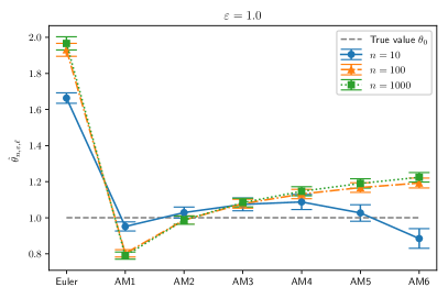
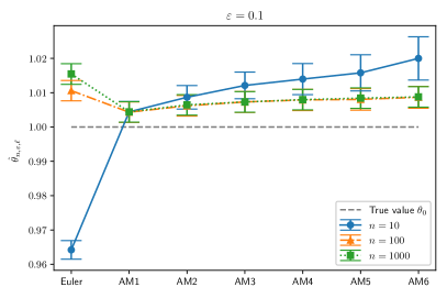
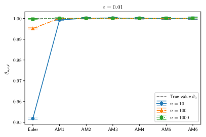
Figure 4.1:

The means and 95% confidence intervals through 10,000

iteration for $\hat{\theta}_{n,\varepsilon}$ (Euler) and $\hat{\theta}_{n,\varepsilon,\ell}$ (AM$\ell$, $\ell=1,\dots,6$).

Acknowledgements. This research was partially supported by JSPS KAKENHI Grant-in-Aid for Scientific Research (A) #17H01100 and JST CREST #PMJCR14D7, Japan.

Appendix A Appendix

Lemma A.1.

Let $\gamma_{\ell\nu}$ and $\beta_{\ell\nu}$ be given by (1.3) and (1.4). Then,

$$\sum_{\nu=1}^{\ell}\left|\gamma_{\ell\nu}\right|\leq\ell 2^{\ell-1}\quad(\ell=1,2,\dots),\qquad\sum_{\nu=0}^{\ell}\left|\beta_{\ell\nu}\right|\leq 2^{\ell}\quad(\ell=0,1,\dots).$$ (A.1)

Proof.

The conclusion is obtained from

$$\sum_{\nu=1}^{\ell}\left|\gamma_{\ell\nu}\right|=\sum_{\nu=1}^{\ell}\frac{1}{(\nu-1)!(\ell-\nu)!}\int_{0}^{1}\prod_{\begin{subarray}{c}j=1\\ j\neq\nu\end{subarray}}^{\ell}(u+j-1)\,du\leq\sum_{\nu=1}^{\ell}\frac{\ell!}{(\nu-1)!(\ell-\nu)!}=\ell 2^{\ell-1}$$ (A.2)

for $\ell=1,2\dots$, and

$$\sum_{\nu=0}^{\ell}\left|\beta_{\ell\nu}\right|=\sum_{\nu=0}^{\ell}\frac{1}{\nu!(\ell-\nu)!}\int_{0}^{1}\prod_{\begin{subarray}{c}j=0\\ j\neq\nu\end{subarray}}^{\ell}(u+j-1)\,du\leq\sum_{\nu=0}^{\ell}\frac{\ell!}{\nu!(\ell-\nu)!}=2^{\ell}$$ (A.3)

for $\ell=0,1,\dots$. ∎

Lemma A.2.

Let $g$ be a continuous function on $\mathbb{R}^{d}$, let $t\mapsto y_{t}$ be an $\mathbb{R}^{d}$-valued continuous function on $[0,1]$, and let $\{f(\cdot,\theta)\}_{\theta\in\Theta}$ be a pointwise equicontinuous family of functions from $\mathbb{R}^{d}$ to $\mathbb{R}^{d}$. If $\ell/n\to 0$ as $n\to\infty$, then

$$\frac{1}{n}\sum_{k=\ell\vee 1}^{n}g\left(\mathchoice{{\vbox{\hbox{$\textstyle-$}}\kern-4.86108pt}}{{\vbox{\hbox{$\scriptstyle-$}}\kern-3.25pt}}{{\vbox{\hbox{$\scriptscriptstyle-$}}\kern-2.29166pt}}{{\vbox{\hbox{$\scriptscriptstyle-$}}\kern-1.875pt}}\!\int_{t_{k-1}}^{t_{k}}f(y_{t},\theta)\,dt\right)\to\int_{0}^{1}g\circ f(y_{t},\theta)\,dt$$ (A.4)

as $n\to\infty$, uniformly in $\theta\in\Theta$.

Proof.

Since $\{f(y_{\cdot},\theta)\}_{\theta\in\Theta}$ is uniformly equicontinuous on $[0,1]$, for any $\eta>0$ there exists $N\in\mathbb{N}$ such that $\theta\in\Theta$, $|s-t|\leq 1/N$ $\Rightarrow$ $\left|f(y_{s},\theta)-f(y_{t},\theta)\right|<\eta$. Then, for all $n\geq N$, $t\in[0,1)$ and $\theta\in\Theta$

$$\left|\sum_{k=1}^{n}\boldsymbol{1}_{[t_{k-1},t_{k})}(t)\,\mathchoice{{\vbox{\hbox{$\textstyle-$}}\kern-4.86108pt}}{{\vbox{\hbox{$\scriptstyle-$}}\kern-3.25pt}}{{\vbox{\hbox{$\scriptscriptstyle-$}}\kern-2.29166pt}}{{\vbox{\hbox{$\scriptscriptstyle-$}}\kern-1.875pt}}\!\int_{t_{k-1}}^{t_{k}}f(y_{s},\theta)\,ds-f(y_{t},\theta)\right|\leq\sum_{k=1}^{n}\boldsymbol{1}_{[t_{k-1},t_{k})}(t)\,\mathchoice{{\vbox{\hbox{$\textstyle-$}}\kern-4.86108pt}}{{\vbox{\hbox{$\scriptstyle-$}}\kern-3.25pt}}{{\vbox{\hbox{$\scriptscriptstyle-$}}\kern-2.29166pt}}{{\vbox{\hbox{$\scriptscriptstyle-$}}\kern-1.875pt}}\!\int_{t_{k-1}}^{t_{k}}\left|f(y_{s},\theta)-f(y_{t},\theta)\right|\,ds<\eta,$$ (A.5)

and we have

$$\sum_{k=1}^{n}\boldsymbol{1}_{[t_{k-1},t_{k})}(t)\,\mathchoice{{\vbox{\hbox{$\textstyle-$}}\kern-4.86108pt}}{{\vbox{\hbox{$\scriptstyle-$}}\kern-3.25pt}}{{\vbox{\hbox{$\scriptscriptstyle-$}}\kern-2.29166pt}}{{\vbox{\hbox{$\scriptscriptstyle-$}}\kern-1.875pt}}\!\int_{t_{k-1}}^{t_{k}}f(y_{s},\theta)\,ds\to f(y_{t},\theta)$$ (A.6)

uniformly in $(t,\theta)\in[0,1)\times\Theta$. By the continuity of $g$, we obtain

$$\frac{1}{n}\sum_{k=1}^{n}g\left(\mathchoice{{\vbox{\hbox{$\textstyle-$}}\kern-4.86108pt}}{{\vbox{\hbox{$\scriptstyle-$}}\kern-3.25pt}}{{\vbox{\hbox{$\scriptscriptstyle-$}}\kern-2.29166pt}}{{\vbox{\hbox{$\scriptscriptstyle-$}}\kern-1.875pt}}\!\int_{t_{k-1}}^{t_{k}}f(y_{t},\theta)\,dt\right) =\int_{0}^{1}\sum_{k=1}^{n}\boldsymbol{1}_{[t_{k-1},t_{k})}(t)\,g\left(\mathchoice{{\vbox{\hbox{$\textstyle-$}}\kern-4.86108pt}}{{\vbox{\hbox{$\scriptstyle-$}}\kern-3.25pt}}{{\vbox{\hbox{$\scriptscriptstyle-$}}\kern-2.29166pt}}{{\vbox{\hbox{$\scriptscriptstyle-$}}\kern-1.875pt}}\!\int_{t_{k-1}}^{t_{k}}f(y_{s},\theta)\,ds\right)dt$$ (A.7)

$$=\int_{0}^{1}g\left(\sum_{k=1}^{n}\boldsymbol{1}_{[t_{k-1},t_{k})}(t)\,\mathchoice{{\vbox{\hbox{$\textstyle-$}}\kern-4.86108pt}}{{\vbox{\hbox{$\scriptstyle-$}}\kern-3.25pt}}{{\vbox{\hbox{$\scriptscriptstyle-$}}\kern-2.29166pt}}{{\vbox{\hbox{$\scriptscriptstyle-$}}\kern-1.875pt}}\!\int_{t_{k-1}}^{t_{k}}f(y_{s},\theta)\,ds\right)dt\to\int_{0}^{1}g\circ f(y_{t},\theta)\,dt$$

as $n\to\infty$, uniformly in $\theta\in\Theta$. Since $\{g\circ f(y_{\cdot},\theta)\}_{\theta\in\Theta}$ is equicontinuous at $t=0$, for $\ell\geq 2$,

$$\frac{1}{n}\sum_{k=1}^{\ell-1}g\left(\mathchoice{{\vbox{\hbox{$\textstyle-$}}\kern-4.86108pt}}{{\vbox{\hbox{$\scriptstyle-$}}\kern-3.25pt}}{{\vbox{\hbox{$\scriptscriptstyle-$}}\kern-2.29166pt}}{{\vbox{\hbox{$\scriptscriptstyle-$}}\kern-1.875pt}}\!\int_{t_{k-1}}^{t_{k}}f(y_{t},\theta)\,dt\right)\to 0$$ (A.8)

as $\ell/n\to 0$, uniformly in $\theta\in\Theta$. ∎

Let $(\Omega,P,\mathscr{F})$ be a probability space, and let $\operatorname{Sym}_{p}(\mathbb{R})$ denote the set of all $p\times p$ symmetric matrix with real entries and with the Frobenius norm $\|\cdot\|_{F}$.

Lemma A.3.

Suppose that $v_{n}\overset{p}{\to}v$ in $\mathbb{R}^{p}$ and $M_{n}\overset{p}{\to}M$ in $\operatorname{Sym}_{p}(\mathbb{R})$ as $n\to\infty$, $w_{n}$ satisfies $v_{n}=M_{n}w_{n}$. If $M$ is positive definite, $w_{n}\overset{p}{\to}M^{-1}v$.

Proof.

Let $\eta$ be an arbitrary positive number less than the smallest eigenvalue of $M$. If $\|M_{n}-M\|_{F}<\eta$, then $0\prec M-\eta\mathbb{I}_{p\times p}\prec M_{n}\prec M+\eta\mathbb{I}_{p\times p}$, where $\mathbb{I}_{p\times p}$ is the identity matrix of size $p$ and $\prec$ is the Loewner order. This implies that $M_{n}$ is invetible and

$$\left(M+\eta\mathbb{I}_{p\times p}\right)^{-1}\prec M_{n}^{-1}\prec\left(M-\eta\mathbb{I}_{p\times p}\right)^{-1}.$$ (A.9)

Since $(M\pm\eta\mathbb{I}_{p\times p})^{-1}\to M^{-1}$ in $\operatorname{Sym}_{p}(\mathbb{R})$ as $\eta\to 0$, there exists a positive number $\tilde{\eta}$ depending only on $M,p$ and $\eta$ such that $\|M_{n}^{-1}-M^{-1}\|_{F}<\tilde{\eta}$ and $\tilde{\eta}\to 0$ as $\eta\to 0$.

Set $\mathscr{D}_{n}:=\{\omega\in\Omega\,|\,M_{n}(\omega)~{}\text{is invertible}\}$. Then, if an arbitrary positive number $\tilde{\eta}$ is sufficiently small, for some $\eta>0$ we have

$$P(\mathscr{D}_{n}^{\mathrm{C}})+P(\boldsymbol{1}_{\mathscr{D}_{n}}\|M_{n}^{-1}-M^{-1}\|_{F}>\tilde{\eta})\leq 2P(\|M_{n}^{-1}-M^{-1}\|_{F}>\eta)\to 0,$$ (A.10)

where $\boldsymbol{1}_{A}$ is the indicator function on a set $A\subset\Omega$. Hence, we obtain

$$w_{n}=M_{n}^{-1}v_{n}\boldsymbol{1}_{\mathscr{D}_{n}}+w_{n}\boldsymbol{1}_{\mathscr{D}_{n}^{\mathrm{C}}}\overset{p}{\to}M^{-1}v$$ (A.11)

as $n\to\infty$. ∎

References

• [1] David Applebaum, Lévy processes and stochastic calculus, second ed., Cambridge Studies in Advanced Mathematics, vol. 116, Cambridge University Press, Cambridge, 2009.
• [2] J. C. Butcher, Numerical methods for ordinary differential equations, third edition ed., John Wiley & Sons, Ltd., Chichester, 2016.
• [3] Philip J. Davis, Interpolation and approximation. republication, with minor corrections, of the 1963 original, with a new preface and bibliography, Dover Publications, Inc., New York, 1975.
• [4] Lawrence C. Evans, Partial differential equations, second ed., Graduate Studies in Mathematics, vol. 19, American Mathematical Society, Providence, RI, 2010.
• [5] V. Genon-Catalot, Maximum contrast estimation for diffusion processes from discrete observations, Statistics 21 (1990), no. 1, 99–116.
• [6] E. Hairer, S. P. Nørsett, and G. Wanner, Solving ordinary differential equations. i. nonstiff problems, second ed., Springer Series in Computational Mathematics, vol. 8, Springer-Verlag, Berlin, 1993.
• [7] E. Hairer and G. Wanner, Solving ordinary differential equations. ii. stiff and differential-algebraic problems, second revised ed., Springer Series in Computational Mathematics, vol. 14, Springer-Verlag, Berlin, 2010.
• [8] A. Iserles, A first course in the numerical analysis of differential equations, 2 ed., Cambridge Texts in Applied Mathematics, Cambridge University Press, 2008.
• [9] Catherine F. Laredo, A sufficient condition for asymptotic sufficiency of incomplete observations of a diffusion process, Ann. Statist. 18 (1990), no. 3, 1158–1171.
• [10] H. Long, Y. Shimizu, and W. Sun, Least squares estimators for discretely observed stochastic processes driven by small Lévy noises, J. Multivariate Anal. 116 (2013), 422–439.
• [11] Hongwei Long, Chunhua Ma, and Yasutaka Shimizu, Least squares estimators for stochastic differential equations driven by small lévy noises, Stochastic Process. Appl. 127 (2017), no. 5, 1475–1495.
• [12] Xuerong Mao, Stochastic differential equations and applications, second ed., Horwood Publishing Limited, Chichester, 2008.
• [13] T. Ogihara and N. Yoshida, Quasi-likelihood analysis for the stochastic differential equation with jumps, Stat. Inference Stoch. Process 14 (2011), no. 3, 189–229.
• [14] Yasutaka Shimizu, Threshold estimation for stochastic processes with small noise, Scand. J. Stat. 44 (2017), no. 4, 951–988.
• [15] Michael Sørensen and Masayuki Uchida, Small-diffusion asymptotics for discretely sampled stochastic differential equations, Bernoulli 9 (2003), no. 6, 1051–1069.
• [16] Masayuki Uchida, Estimation for discretely observed small diffusions based on approximate martingale estimating functions, Scand. J. Statist. 31 (2004), no. 4, 553–566.
• [17] A. W. van der Vaart, Asymptotic statistics, Cambridge Series in Statistical and Probabilistic Mathematics, vol. 3, Cambridge University Press, Cambridge, 1998.