Asymptotic self-similar blow-up profile for three-dimensional axisymmetric Euler equations using neural networks

Abstract

Whether there exist finite time blow-up solutions for the 2-D Boussinesq and the 3-D Euler equations are of fundamental importance to the field of fluid mechanics. We develop a new numerical framework, employing physics-informed neural networks (PINNs), that discover, for the first time, a smooth self-similar blow-up profile for both equations. The solution itself could form the basis of a future computer-assisted proof of blow-up for both equations. In addition, we demonstrate PINNs could be successfully applied to find unstable self-similar solutions to fluid equations by constructing the first example of an unstable self-similar solution to the Córdoba-Córdoba-Fontelos equation. We show that our numerical framework is both robust and adaptable to various other equations.

A celebrated open question in fluids is whether or not from smooth initial data the 3-D Euler equations may develop finite-time singularities (the inviscid analogue of the Navier-Stokes Millennium-prize problem). For non-smooth $C^{1,\alpha}$ initial data with $0<\alpha\ll 1$, finite-time self-similar blow-up was proven in the groundbreaking work of Elgindi [1, 2]. The question of finite-time blow-up from smooth initial data remains unresolved.

In the presence of a cylindrical boundary, Luo and Hou [3] (cf. [4]) performed compelling numerical simulations proposing a scenario – sharing similarities with Pumir and Siggia [5] (cf. [6, 7]) – for finite time blow-up of the axi-symmetric 3-D Euler equations. They simulated the time-dependent problem and observed a dramatic growth in the maximum of vorticity (by a factor of $3\cdot 10^{8}$), strongly suggesting formation of a singularity. The work is also suggestive of asymptotic self-similarity.

To confirm the existence of the finite-time singularity in the Luo-Hou scenario, and find its self-similar structure, we need to solve the self-similar equations associated with the axisymmetric 3-D Euler equations in the local coordinates near the singularity, which poses an extreme challenge to classical numerical methods as explained later. In this Letter, we develop a new numerical strategy, based on Physics-informed Neural Networks (PINNs) that can solve the self-similar equations in a simple and robust way. This new method allows us, for the first time, to find the smooth asymptotic self-similar blow-up profile for the Luo-Hou scenario. To the best of our knowledge, the solution is also the first truly multi-dimensional smooth backwards self-similar profile for an equation from fluid mechanics.

Singularity formation for 3-D Euler equations with a cylindrical boundary is intrinsically linked to the same problem for the 2-D Bousinessq equations (cf. [4, 8, 9, 10]), another fundamental question in fluid mechanics, mentioned in Yudovich’s ‘Eleven great problems of mathematical hydrodynamics’ [11]. The mechanism for blow-up for the two equations is believed to be identical. The 2-D Boussinesq equations take the form

$$\begin{gathered}\partial_{t}{\bf u}+{\bf u}\cdot\nabla{\bf u}+\nabla p=(0,\theta),\\ \partial_{t}\theta+{\bf u}\cdot\nabla\theta=0,~{}\mathrm{div\,}{\bf u}=0\,,\end{gathered}$$ (1)

where the 2-D vector ${\bf u}({\bf x},t)$ is the velocity and the scalar $\theta({\bf x},t)$ is the temperature. We consider the spatial variable ${\bf x}=(x_{1},x_{2})$ to be taken on the half plane $x_{2}\geq 0$ and impose a non-penetration boundary condition at $x_{2}=0$ ($x_{1}$-axis), namely $u_{2}(x_{1},0)=0$.

To search for singularity formation for the Boussinesq equations (1), we look for backwards self-similar solutions of the form ${\bf u}=(1-t)^{\lambda}{\bf U}({\bf y})$ and $\theta=(1-t)^{-1+\lambda}\Theta({\bf y})$, where we define the self-similar coordinates as ${\bf y}=(y_{1},y_{2})=\tfrac{(x_{1},x_{2})}{(1-t)^{1+\lambda}}$ with ${\lambda>-1}$ yet to be determined. Under such a self-similar ansatz, the equations (1) become

$$\begin{gathered}-\lambda{\bf U}+((1+\lambda){\bf y}+{\bf U})\cdot\nabla{\bf U}+\nabla P=(0,\Theta)\,,\\ (1-\lambda)\Theta+((1+\lambda){\bf y}+{\bf U})\cdot\nabla\Theta=0,~{}\mathrm{div\,}{\bf U}=0\,.\end{gathered}$$ (2)

The corresponding solution is expected to have infinite energy [13]; however, we impose that the solution to (2) has mild growth at infinity (see cost functions in Supplementary Material) which is an essential requirement for such a solution to be cut-off to produce an asymptotically self-similar solution with a finite energy.

Setting $\Omega=\mathrm{curl\,}{\bf U}=\partial_{y_{1}}U_{2}-\partial_{y_{2}}U_{1}$, $\Phi=\partial_{y_{1}}\Theta$ and $\Psi=\partial_{y_{2}}\Theta$, we rewrite (2) in vorticity form

$$\begin{split}\Omega+((1+\lambda){\bf y}+{\bf U})\cdot\nabla\Omega&=\Phi\,,\\ (2+\partial_{y_{1}}U_{1})\Phi+((1+\lambda){\bf y}+{\bf U})\cdot\nabla\Phi&=-\partial_{y_{1}}U_{2}\Psi\,,\\ (2+\partial_{y_{2}}U_{2})\Psi+((1+\lambda){\bf y}+{\bf U})\cdot\nabla\Psi&=-\partial_{y_{2}}U_{1}\Phi\,,\\ \mathrm{div\,}{\bf U}&=0\,.\end{split}$$ (3)

To help find the solution, we impose the symmetries: ($U_{1},\Phi,\Omega$) are odd and $(U_{2},\Psi)$ are even in the $y_{1}$ direction. In addition, we impose $U_{2}(y_{1},0)=0$ (the non-penetration boundary condition). To guarantee the uniqueness of the solution (removing scaling symmetry), we constrain $\partial_{y_{1}}\Omega(0,0)=-1$. Finally, to rule out extraneous solutions, we impose that $\nabla{\bf U}$, $\Phi$ and $\Psi$ all vanish at infinity.

To describe the Luo-Hou scenario for the 3-D Euler blow-up in the presence of boundary, we write the axisymmetric 3-D Euler equations:

$$\begin{split}\left(\partial_{t}+u_{r}\partial_{r}+u_{3}\partial_{x_{3}}\right)\left(\tfrac{\omega_{\theta}}{r}\right)&=\tfrac{1}{r^{4}}\partial_{x_{3}}\left(ru_{\theta}\right)^{2}\\ \left(\partial_{t}+u_{r}\partial_{r}+u_{3}\partial_{x_{3}}\right)\left(ru_{\theta}\right)&=0\end{split}$$ (4)

where $(u_{r},u_{\theta},u_{3})$ is the velocity in cylindrical coordinates and $\omega_{\theta}$ is the angular component of the vorticity. We introduce a cylindrical boundary at $r=1$, and restrict to the exterior domain $\{(r,x_{3})\in r\geq 1,x_{3}\in\mathbb{R}\}$. By imposing the self-similar ansatz $(u_{x_{3}},u_{r})=(1-t)^{\lambda}{\bf U}({\bf y},s)$, $\omega_{\theta}=(1-t)^{-1}\Omega({\bf y},s)$, $\partial_{r}\left(ru_{\theta}\right)^{2}=(1-t)^{-2}\Psi({\bf y},s)$ and $\partial_{x_{3}}\left(ru_{\theta}\right)^{2}=(1-t)^{-2}\Phi({\bf y},s)$ for self-similar coordinates ${\bf y}=(y_{1},y_{2})=\tfrac{(x_{3},r-1)}{(1-t)^{1+\lambda}}$ and $s=-\log(1-t)$, the 3-D Euler equation (4) becomes

$$({\partial_{s}}+\Omega)+((1+\lambda){\bf y}+{\bf U})\cdot\nabla\Omega =\Phi+\mathcal{E}_{1}$$

$$({\partial_{s}}+2+\partial_{y_{1}}U_{1})\Phi+((1+\lambda){\bf y}+{\bf U})\cdot\nabla\Phi =-\partial_{y_{1}}U_{2}\Psi$$

$$({\partial_{s}}+2+\partial_{y_{2}}U_{2})\Psi+((1+\lambda){\bf y}+{\bf U})\cdot\nabla\Psi =-\partial_{y_{2}}U_{1}\Phi$$

$$\mathrm{div\,}{\bf U} =\mathcal{E}_{2}$$ (5)

where the errors $\mathcal{E}_{1}$ and $\mathcal{E}_{2}$ are given by the expressions

$$\small\mathcal{E}_{1} {\tiny=-y_{2}e^{-(1+\lambda)s}\tfrac{(y_{2}e^{-(1+\lambda)s}+2)(y_{2}^{2}e^{-2(1+\lambda)s}+2y_{2}e^{-(1+\lambda)s}+2)}{(1+y_{2}e^{-(1+\lambda)s})^{4}}\Phi}$$

$$\mathcal{E}_{2} {\tiny=-e^{-(1+\lambda)s}\tfrac{U_{2}}{1+y_{2}e^{-(1+\lambda)s}}\,.}$$

We look for solutions which are asymptotically self-similar: i.e. in self-similar coordinates they converge to a stationary state as $s\rightarrow\infty$. For such solutions, at any fixed ${\bf y}$, we have $\mathcal{E}_{1},\mathcal{E}_{2}=O(e^{-(1+\lambda)s})$ and thus the errors decay exponentially fast in self-similar coordinates assuming that $\lambda>-1$. Thus, the self-similar equations (5) for Euler converge to Bousinessq (3) as $s\rightarrow\infty$. Namely, the self-similar solution for Boussinesq is identical to the asymptotic self-similar blow-up profile to Euler with cylindrical boundary.

A key difficulty of solving the equation (3) lies in the unknown parameter $\lambda$ that needs to be solved simultaneously. We search for smooth non-trivial solutions to (3), which exist for discrete $\lambda$ values. This problem is extremely challenging using classical evolution (time-dependent) based numerical methods (cf. [16, 17, 18, 3, 4, 19, 20]).

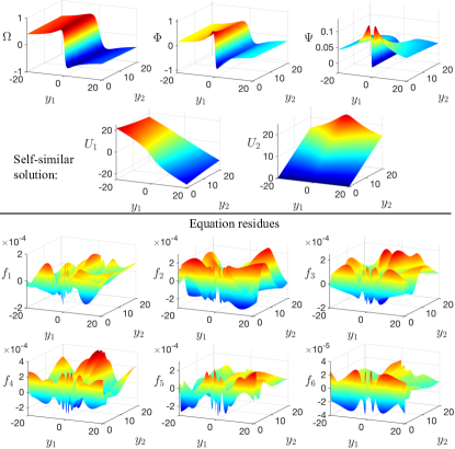
Figure 1: Solution for (3) found by PINN. $f_{i}$ indicate the residues, which are of five orders of magnitude smaller than the solution. The inferred value of $\lambda$ is $1.917\pm 0.002$ after systematic test (see Supplementary Material).

Physics-informed neural networks (PINNs) were recently developed  [21, 22] as a new class of numerical solver for PDEs and have been widely used in science and engineering [23]. In PINNs, neural networks approximate the solution to a PDE by searching for a solution in a continuous domain that approximately satisfies the physics constraints (e.g. equations and solution constraints). PINNs have been successfully used to solve not only forward problems but also inverse problems (e.g. identifying the Reynolds number from a given flow and the Navier-Stokes equation [21]), demonstrating the capacity of PINNs to invert for unknown parameters in the governing equations. Here, we use a PINN to find not only the self similar solution profile but also the unknown self-similarity exponent $\lambda$. To guarantee the success of PINN, it is critical to understand the key symmetries of the problem, its spurious solutions, as well as intuition of the qualitative properties of the solution (e.g. its geometry and asymptotics).

To find the self-similar solution for the Bousinessq equation, we represent each of $U_{1}$, $U_{2}$, $\Omega$, $\Phi$ or $\Psi$ in the Bousinessq equations (3) by an individual fully-connected neural network with $y_{1}$ and $y_{2}$ as its inputs. We use 6 hidden layers with 30 units in each hidden layer for each network and use the hyperbolic tangent function $\tanh$ as the activation function. We impose the symmetry of each variable ($U_{1},U_{2},\Omega,\Phi,\Psi$) by constructing the function form $q_{odd}=[\mathrm{NN}_{q}(y_{1},y_{2})-\mathrm{NN}_{q}(-y_{1},y_{2})]/2$ and $q_{even}=[\mathrm{NN}_{q}(y_{1},y_{2})+\mathrm{NN}_{q}(-y_{1},y_{2})]/2$, where $\mathrm{NN}_{q}$ is the neural network created for the variable $q$.

To train the neural network, we need a cost function and an optimization algorithm. For PINNs, the cost function is composed of two types of loss. The first is the condition loss, which evaluates the residue of the solution condition, where the residue here is defined as the difference between the neural network approximated condition and the true solution condition. The condition loss can be written as

$$loss_{c}^{(j)}=\frac{1}{N_{c}^{(j)}}\sum_{i=1}^{N_{c}^{(j)}}g_{(j)}^{2}\left[{\bf y}_{i},\hat{q}\left({\bf y}_{i}\right)\right],$$ (6)

where $g_{(j)}\left({\bf y}_{i},\hat{q}({\bf y}_{i})\right)$ indicates the residue of the $j$-th boundary condition at the $i$-th position ${\bf y}_{i}=(y_{1},y_{2})_{i}$ and $\hat{q}\left({\bf y}_{i}\right)$ indicates the neural network prediction of the variable $q$. The parameter $N_{c}^{(j)}$ indicates the total number of points used for evaluating the $j$-th boundary condition.

The second type of loss is known as the equation loss, which evaluates the residue of the governing equation averaged over a set of collocation points over the domain. The residue of the equation $f_{(k)}$ is defined as the error in the equation calculated with the neural network predictions. The equation loss can be written as

$$loss_{f}^{(k)}=\tfrac{1}{N_{f}^{(k)}}\sum_{i=1}^{N_{f}^{(k)}}f_{(k)}^{2}\left[{\bf y}_{i},\hat{q}\left({\bf y}_{i}\right)\right],$$ (7)

where $f_{(k)}\left({\bf y_{i}},\hat{q}({\bf y}_{i})\right)$ indicates the residue of the $k$-th equation evaluated at the $i$-th collocation point. The parameter $N_{f}^{(k)}$ denotes the total number of collocation points used for the $k$-th equation. The residues of the boundary conditions $g_{(j)}$ and equations $f_{(k)}$ involved in the cost function are listed in the Supplemental Material.

We stress that all equations are local, which is an advantage of our method versus alternate methods that require a careful consideration of non-locality in infinite domains. In our implementation, to approximate an infinite domain, we introduce the coordinates $z=(z_{1},z_{2})=(\sinh^{-1}(y_{1}),\sinh^{-1}(y_{2}))$ (see Figure 2$a$) and consider a domain $z\in[-30,30]^{2}$. In the $y$-coordinates, this corresponds to a domain $\approx[-5\cdot 10^{12},5\cdot 10^{12}]^{2}$. The equations written in $z$-coordinates are given in the Supplemental Material.

The equations and conditions provided so far can only find the unique solution to (3) for a specified $\lambda$. Figure 1 in the Supplementary Material shows the PINN solution to (3) for $\lambda=3$. The large equation residue at the origin indicates the non-smoothness of the solution at the origin (see Supplemental Material). To search for the right $\lambda$ that guarantees the smoothness of solutions, i.e. avoiding the local peaks in the equation residue, we impose the smoothness constraint to penalize the gradient of equation residues around the non-smooth point (origin).

$$loss_{s}^{(k)}=\frac{1}{N_{s}^{(k)}}\sum_{i=1}^{N_{s}^{(k)}}\left|\nabla f_{(k)}\left({\bf y}_{i},\bar{q}\left({\bf y}_{i}\right)\right)\right|^{2}\,,$$ (8)

where $N_{s}^{(k)}$ indicates the total number of collocation points close to the origin. The sum of (6), (7) and (8) defines the final cost function

$$J({\bf y,w})=\tfrac{1}{n_{b}}\sum_{j=1}^{n_{b}}loss_{c}^{(j)}+\gamma(\tfrac{1}{n_{e}}\sum_{k=1}^{n_{e}}loss_{f}^{(k)}+\tfrac{1}{n_{e}}\sum_{k=1}^{n_{e}}loss_{s}^{(k)})$$

where $n_{b}=8$ and $n_{e}=6$ are the total number of solution conditions and governing equations used (see Supplementary Material). The constant $\gamma$ is a hyper-parameter of PINNs, known as the equation weight [24], which balances the contribution of the condition loss and equation loss in the final cost function $J({\bf y,w})$. For Boussinesq, we choose $\gamma=0.1$ for optimal training performance.

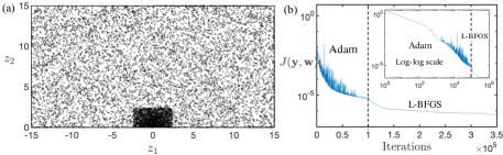
Figure 2: (a) Spatial distribution of the collocation points. Here ($z_{1}$, $z_{2}$) are the rescaled coordinates: $y_{1}=\sinh(z_{1})$ and $y_{2}=\sinh(z_{2})$. 10,000 collocation points in total are used for training. (b) Decrease of the total loss over the training iterations. The inset shows the loss curve in a log-log scale.

The common optimization methods used for PINN training are Adam [25] and L-BFGS [26]. Despite the fact that no optimization method guarantees the convergence to a global minimum, our empirical experience, consistent with prior studies [27], shows that Adam performs better at avoiding local minima, while L-BFGS has a faster convergence rate throughout the training. Thus, we use Adam first for 100,000 iterations and then L-BFGS for 250,000 iterations to search for the self-similar solution for the Bousinessq equations. Figure 2(b) shows the convergence of the cost function $J({\bf y,w})$ throughout the training iterations.

Figure 1 shows the approximate solutions to (3), along with their corresponding equation residues. The equation residues are approximately five orders of magnitude smaller than that of the solution found. With the smoothness constraint (8) the inferred exponent for the smooth solution is $\lambda\approx 1.917$. In the Supplementary Material we show the robustness of the PINN prediction with different random initialization and normalization condition. We also demonstrate convergence of the inferred $\lambda$ with domain size. The solutions found by the PINN are in agreement with the asymptotics of the time dependent solutions found by Luo and Hou [3, 4]. Extrapolating from the paper [4], the work is suggestive of a self-similarity exponent of $\lambda\approx 1.9$, in agreement with the exponent found by the PINN. Similarly to Luo and Hou, the trajectories corresponding to the self-similar velocity follow the geometry of a hyperbolic point at the origin.

The spatial distribution of the collocation points plays a critical role for the success of PINN training. To guide the neural network to find the correct self-similar solution for Bousinessq (3), we train the neural network to prioritize the equation constraints around the origin. Towards this goal, we divide the domain into two regions, one close to the origin and one far, in each region the collocation points are uniformly distributed. We increase the number of collocation points surrounding the origin. Otherwise, the neural network prediction would likely be trapped in a local minimum during the training.

The PINN-based scheme for finding self-similar blow-up offers advantages in terms of both universality and efficiency. For universality, the above PINN scheme can be generally applied to solving various self-similar equations without the requirement of prior knowledge of specific structure. For efficiency, the smooth self-similar solution was in fact found by PINN throughout one single training. There is no continuation scheme or time evolution required for the training, largely reducing the computational cost of the method. An additional major advantage of the PINN scheme, as we will later demonstrate, is its ability to find unstable self-similar solutions which would be incredibly difficult, if not impossible to find via traditional methods.

To validate our approach, we compare self-similar solutions obtained to known results in the literature (Supplementary Material). We apply the PINN scheme to find non-smooth solutions to the Boussinesq equation, which are in agreement with the explicit approximate solutions of Chen and Hou [10] (Section 1.5 of the Supplementary Material).

One of the simplest PDEs exhibiting self-similar blow-up is the 1-D Burgers’ equation, which can be solved analytically. The equation provides an excellent sandbox to test and refine the PINN. Section 2 of the Supplementary Material shows that the PINN scheme can find stable, unstable and non-smooths self-similar solutions to the Burgers’ equation. A common numerical strategy to finding self-similar solutions is to introduce time dependence into the problem: while this is straightforward in the stable case, instabilities in the unstable case make finding unstable self-similar profiles comparatively more difficult, if not impossible. The PINN scheme does not suffer this drawback and thus presents itself as a great method for finding unstable smooth self-similar solutions. This later fact will be reinforced below where we demonstrate that the PINN is successful in finding new unstable self-similar solutions that have applicability to an important open problem in mathematical fluid dynamics.

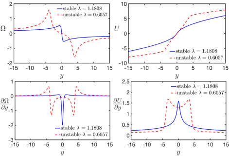
Figure 3: Comparison between stable and unstable solutions with associated $\lambda$ for CCF equation.

The generalized De Gregorio equation [28] is given by

$$\omega_{t}+au\omega_{x}=\omega u_{x},\quad\mbox{where }u=\smallint_{0}^{x}H\omega=\Lambda^{-1}\omega$$

and $H$ is the Hilbert transform. The equation is a generalization of the De Gregorio equation ($a=1$) [29] and has been proposed as a one-dimensional model for an equation for which there is nontrivial interaction of advection and vortex stretching (modeling behavior of the 3-D Euler equations).

The case $a=0$, in the absence of advection, is known in the literature as the Constantin-Lax-Majda equation. In this simple case, exact self-similar blow-up solutions can be constructed [30]. The case $a=-1$ (known as the Córdoba-Córdoba-Fontelos (CCF) model) was proposed as a model of the surface quasi-geostrophic (SQG) equation and it also develops finite time singularities [31]. In the case $a<0$, advection and vortex stretching work in conjunction leading to finite time singularities [32]. The case $a>0$ leads to the competition of the two terms. By a clever expansion in $a$, smooth self-similar profiles were constructed in [33] for small, positive $a$, leading to finite time blow-up. Via a computer-assisted proof, Chen, Hou, and Huang in [34] proved blow-up for the De Gregorio equation ($a=1$).

Lushnikov et al. [35] represents the most thorough numerical study of the generalized De Gregorio equation to date. In [35], self-similar solutions were found in the whole range $a\in[-1,1]$ and beyond. We use their reported parameters as benchmarks for our results. In the Supplementary Material , we show that PINN can accurately reproduce the findings of [35].

Returning to the specific case of CCF ($a=-1$), an interesting question to add fractional dissipation $(-\Delta)^{\alpha/2}$ and ask for which values of $\alpha$ do singularities occur. Blow-up is known to occur for $0\leq\alpha<\frac{1}{2}$, whereas for $\alpha\geq 1$ the problem is global-wellposed [37, 38, 39]. The behavior in the range $\frac{1}{2}\leq\alpha<1$ remains an important open problem.

Assuming the ansatz $\omega=\tfrac{1}{1-t}\Omega(\tfrac{x}{(1-t)^{1+\lambda}},s)$ for $s=-\log(1-t)$, then in the self-similar evolution equation for $\Omega$, the dissipative term takes the form $e^{((1+\lambda)\alpha-1)s}(-\Delta)^{\frac{\alpha}{2}}\Omega$. Analogous to how self-similar Boussinesq solutions can be used to construct asymptotically self-similar solutions to Euler with boundary, self-similar inviscid CCF solutions satisfying the condition $(1+\lambda)\alpha-1<0$ may be employed to construct asymptotically self-similar solutions to dissipative CCF. Since $\lambda\approx 1.18078$ for the stable self-similar solution to inviscid CCF, such a solution is ill-suited to prove blow-up in the parameter range $\frac{1}{2}\leq\alpha<1$. Motivated by known work on the Burgers’ equation [40, 41] and compressible Euler [42, 43], one could conjecture the existence of a discrete hierarchy of unstable solutions with decreasing $\lambda$. By windowing the parameter $\lambda$, including additional derivatives of the governing equation in our residues, and using the constraint $\Omega(0.5)=0.05$ to renormalize, the PINN discovers an unstable self-similar solution corresponding to $\lambda\approx 0.60573$ (see Figure 3). Such a solution would allow us to prove blow-up for dissipative CCF for the range $\alpha<\frac{1}{1+\lambda}\approx 0.61$. Moreover, such a result is suggestive of a possible strategy of addressing the Navier-Stokes Millennium Prize [44], i.e. via unstable self-similar solutions to 3-D Euler (the same strategy has proved successful for dissipative Burgers’ and compressible Navier-Stokes [45, 46, 43]). One expects that the PINN may be adapted to find higher order unstable solutions to CCF as well as unstable solutions to the Boussinesq equation – this is subject of future work.