TaxoCom: Topic Taxonomy Completion with Hierarchical Discovery of Novel Topic Clusters

Abstract.

Topic taxonomies, which represent the latent topic (or category) structure of document collections, provide valuable knowledge of contents in many applications such as web search and information filtering. Recently, several unsupervised methods have been developed to automatically construct the topic taxonomy from a text corpus, but it is challenging to generate the desired taxonomy without any prior knowledge. In this paper, we study how to leverage the partial (or incomplete) information about the topic structure as guidance to find out the complete topic taxonomy. We propose a novel framework for topic taxonomy completion, named TaxoCom, which recursively expands the topic taxonomy by discovering novel sub-topic clusters of terms and documents. To effectively identify novel topics within a hierarchical topic structure, TaxoCom devises its embedding and clustering techniques to be closely-linked with each other: (i) locally discriminative embedding optimizes the text embedding space to be discriminative among known (i.e., given) sub-topics, and (ii) novelty adaptive clustering assigns terms into either one of the known sub-topics or novel sub-topics. Our comprehensive experiments on two real-world datasets demonstrate that TaxoCom not only generates the high-quality topic taxonomy in terms of term coherency and topic coverage but also outperforms all other baselines for a downstream task.

1. Introduction

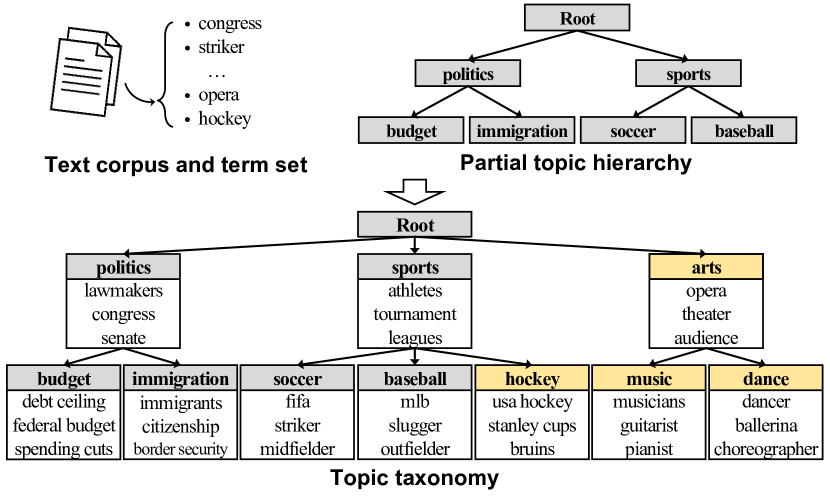
Figure 1. An example of topic taxonomy completion. The known (i.e., given) sub-topics and novel sub-topics are colored in grey and yellow, respectively.

Finding the latent topic structure of an input text corpus, also known as hierarchical topic discovery (Zhang et al., 2018; Shang et al., 2020; Downey et al., 2015; Wang et al., 2013; Liu et al., 2012), has been one of the most important problems for information extraction and semantic analysis of text data. Recently, several studies have focused on topic taxonomy construction (Zhang et al., 2018; Shang et al., 2020), which aims to generate a tree-structured taxonomy whose node corresponds to a conceptual topic; each node of the topic taxonomy is defined as a cluster of semantically coherent terms representing a single topic. Compared to a conventional entity (or term-level) taxonomy, this cluster-level taxonomy is more appropriate for representing the topic hierarchy of the target corpus with high coverage and low redundancy. To identify hierarchical topic clusters of terms, they mainly performed clustering on a low-dimensional text embedding space where textual semantic information is effectively encoded.

However, their output topic taxonomy seems plausible by itself but often fails to match with the complete taxonomy designed by a human curator, because they rely on only the text corpus in an unsupervised manner. To be specific, their quality (e.g., coverage and accuracy) highly depends on the number of sub-topic clusters (i.e., child nodes), which has to be manually controlled by a user. In addition, it is sensitive to the topic imbalance in the document collection, which makes it difficult to find out minor topics. In the absence of any information about the topic hierarchy, the unsupervised methods intrinsically become vulnerable to these problems.

On the other hand, for some other text mining tasks or NLP applications, several recent studies have tried to take advantage of auxiliary information about the latent topic structure (Meng et al., 2020a, c; Meng et al., 2019b; Shen et al., 2021; Huang et al., 2020a; Meng et al., 2020b; Meng et al., 2018). Most of them focus on utilizing a hierarchy of topic surface names as additional supervision, because it can be easily given as a user’s interests or prior knowledge. Specifically, they retrieve the top-$K$ relevant terms to each topic (Meng et al., 2020a, c) or train a hierarchical text classifier using unlabeled documents and the topic names (Meng et al., 2019b; Shen et al., 2021). Despite their effectiveness, their major limitation is that they are only able to consider the known topics included in the given topic hierarchy. That is, the coverage of the obtained results is strictly limited to the given topics. Since it is very challenging for a user to be aware of a full topic structure, a naive solution to incorporate a user-provided hierarchy of topic names into the topic taxonomy is likely to only partially cover the text corpus.

To tackle this limitation, we introduce a new problem setting, named topic taxonomy completion, to construct a complete topic taxonomy by making use of additional topic information assumed to be partial or incomplete. Formally, given a text corpus and its partial hierarchy of topic names, this task aims to identify the term clusters for each topic, while discovering the novel topics that do not exist in the given hierarchy but exist in the corpus. Figure 1 illustrates a toy example of our task, where the novel topics (e.g, arts and hockey) are correctly detected and placed in the right position within the taxonomy. This task can be practically applied not only for the case that a user’s incomplete knowledge is available, but also for incremental management of the topic taxonomy. In case that the document collection is constantly growing, and so are their topics, the out-dated topic taxonomy of the previous snapshot can serve as the partial hierarchy to capture emerging topics.

The technical challenges of this task can be summarized as follows. First, novel topics should be identified by considering the hierarchical semantic relationship among the topics. In Figure 1, the topic hockey is not novel in terms of the root node, because it obviously belongs to its known sub-topic sports. However, hockey should be detected as a novel sub-topic of sports as it does not belong to any of the known sport sub-categories (i.e., soccer and baseball). Second, the granularity of novel sub-topics and that of known sub-topics need to be kept similar with each other, to achieve the consistency of semantic specificity among sibling nodes. In Figure 1, the root node should insert a single novel sub-topic arts, rather than two novel sub-topics music and dance, based on the semantic specificity of its known sub-topics (i.e., politics and sports).

In this work, we propose TaxoCom, a hierarchical topic discovery framework to complete the topic taxonomy by recursively identifying novel sub-topic clusters of terms. For each topic node, TaxoCom performs (i) text embedding and (ii) text clustering, to assign the terms into one of either the existing child nodes (i.e., known sub-topics) or newly-created child nodes (i.e., novel sub-topics). It first optimizes locally discriminative embedding which enforces the discrimination among the known sub-topics (Meng et al., 2020c, a) by using the given topic surface names; this helps to make a clear distinction between known and novel sub-topic clusters as well. Then, it performs novelty adaptive clustering which separately finds the clusters on novel-topic terms and known-topic terms, respectively. In particular, TaxoCom selectively assigns the terms into the child nodes, referred to as anchor terms, while filtering out general terms based on their semantic relevance and representativeness.

Extensive experiments on real-world datasets demonstrate that TaxoCom successfully completes a topic taxonomy with missing (i.e., novel) topic nodes correctly inserted. Our human evaluation quantitatively validates the superiority of topic taxonomies generated by TaxoCom, in terms of the topic coverage as well as semantic coherence among the topic terms. Furthermore, TaxoCom achieves the best performance among all baseline methods for a downstream task, which trains a weakly supervised text classifier by using the topic taxonomy instead of document-level labels.

2. Related Work

Topic Taxonomy Construction.   Early work on hierarchical topic discovery mainly focused on generative probabilistic topic models, such as hierarchical Latent Dirichlet Allocation (hLDA) (Blei et al., 2003a) and hierarchical Pachinko Allocation Model (hPAM) (Mimno et al., 2007). They describe the topic hierarchy in a generative process and then estimate parameters by using inference algorithms, including variational Bayesian inference (Blei et al., 2003b) and collapsed Gibbs sampling (Griffiths and Steyvers, 2004). With the advances in text embedding techniques, several recent studies started to employ hierarchical clustering methods on a term embedding space, where textual semantic information is effectively captured. By doing so, they can construct a topic taxonomy whose node corresponds to a term cluster representing a single topic. Specifically, to find out hierarchical topic clusters, TaxoGen (Zhang et al., 2018) recursively performed text embedding and clustering for each sub-topic cluster, and NetTaxo (Shang et al., 2020) additionally leveraged network-motifs extracted from text-rich networks. However, since all of them are unsupervised methods that primarily utilize the input text corpus, the high-level architecture of their output taxonomies does not usually match well with the one designed by a human.

Entity Taxonomy Expansion.   Recently, there have been several attempts to construct the entity (or term-level) taxonomy from a text corpus by expanding a given seed taxonomy (Shen et al., 2017; Shen et al., 2018; Shen et al., 2020; Huang et al., 2020b; Zeng et al., 2021b; Mao et al., 2020; Yu et al., 2020). Note that the main difference of an entity taxonomy from a topic (or cluster-level) taxonomy is that its node represents a single entity or term, so it mainly focuses on the entity-level semantic relationships. They basically discover new entities that need to be inserted into the taxonomy, by learning the “is-a” (i.e., hypernym-hyponym) relation of parent-child entity pairs in the seed taxonomy. To infer the “is-a” relation of an input entity pair, they train a relation classifier based on entity embeddings (Shen et al., 2018), a pre-trained language model (Huang et al., 2020b), and graph neural networks (GNNs) (Shen et al., 2020). Despite their effectiveness, the entity taxonomy cannot either show the semantic relationships among high-level concepts (i.e., topics or term clusters) or capture term co-occurrences in the documents; this makes its nodes difficult to correspond to the topic classes of documents. Therefore, they are not suitable for expanding the latent topic hierarchy of documents, rather be useful for enhancing a knowledge base.

Novelty Detection for Text Data.   Novelty (or outlier) detection for text data, which aims to detect the documents that do not belong to any of the given (or inlier) topics, has been researched in a wide range of NLP applications. They define the novel-ness (or outlier-ness) based on how far each document is located from semantic regions representing the normality. To this end, most unsupervised detectors measure the local/global density (Breunig et al., 2000; Sathe and Aggarwal, 2016) or estimate the normal data distribution (Zhuang et al., 2017; Ruff et al., 2019; Manolache et al., 2021) in a low-dimensional text embedding space. On the other hand, supervised/weakly supervised novelty detectors (Hendrycks et al., 2020; Lee et al., 2020; Lee et al., 2021; Zeng et al., 2021a; Fouché et al., 2020) also have been developed to fully utilize the auxiliary information about the inlier topics. They further optimize the embedding space to be discriminative among the topics, so as to clearly determine whether a document belongs to each inlier topic. However, none of them considers the hierarchical relationships among the inlier topics, which makes them ineffective to identify novel topics from a large text corpus having a topic hierarchy.

3. Problem Formulation

3.1. Concept Definition

Definition 0 (Topic taxonomy).

A topic taxonomy $\mathcal{H}$ refers to a tree structure about the latent topic hierarchy of terms $\mathcal{T}$ and documents $\mathcal{D}$. Each node $c\in\mathcal{H}$ is described by a cluster of terms $\mathcal{T}_{c}(\subset\mathcal{T})$ representing a single conceptual topic. The most representative term for the node becomes a center term $t_{c}\in\mathcal{T}_{c}$, usually regarded as the topic surface name. The child nodes of each topic node correspond to its sub-topics. For each node $c$, the set of its $K_{c}$ child nodes is denoted by $\mathcal{S}_{c}(\subset\mathcal{H})=\{s_{c,1},\ldots,s_{c,K_{c}}\}$.

3.2. Topic Taxonomy Completion

Definition 0 (Topic taxonomy completion).

The inputs are a text corpus $\mathcal{D}$, its term set $\mathcal{T}$, and a partial hierarchy $\mathcal{H}^{0}$ of topic surface names. The goal of topic taxonomy completion is to complete the topic taxonomy $\mathcal{H}(\supset\mathcal{H}^{0})$ so that it can cover the entire topic structure of the corpus, being guided by the given topic hierarchy. For each node in the taxonomy $c\in\mathcal{H}$, it finds out the set of topic terms $\mathcal{T}_{c}$ that are semantically coherent. In other words, the given topic hierarchy is extended into a larger one by identifying and inserting new topic nodes, while allocating each term into either one of the existing nodes ($\in\mathcal{H}^{0}$) or newly-created nodes ($\in\mathcal{H}\textbackslash\mathcal{H}^{0}$).

Figure 1 shows an example of topic taxonomy completion for a news corpus. Similar to unsupervised topic taxonomy construction (Zhang et al., 2018; Shang et al., 2020), our task works on the set of unlabeled documents whose topic information (e.g., topic class label) is not available. The main difference is that a partial topic hierarchy is additionally provided, which can be a user’s incomplete prior knowledge or an out-dated topic taxonomy of a growing text collection. From the perspective that the given hierarchy serves as auxiliary supervision for discovering the entire topic structure, this task can be categorized as a weakly supervised hierarchical topic discovery.

4. TaxoCom: Proposed Framework

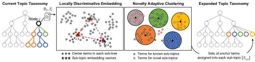
Figure 2. The overview of the TaxoCom framework which discovers the complete topic taxonomy by the recursive expansion of the given topic hierarchy. Starting from the root node, it performs (i) locally discriminative embedding and (ii) novelty adaptive clustering, to selectively assign the terms (of each node) into one of the child nodes. Best viewed in color.

4.1. Overview

The proposed TaxoCom framework recursively expands the given hierarchy in a top-down approach. Starting from the root node, TaxoCom performs (i) text embedding and (ii) text clustering for each node, to find out sub-topic clusters corresponding to its child nodes. The key challenge here is to identify the term clusters for known (i.e., given) sub-topics as well as novel sub-topics, which cannot be covered by any of the known sub-topics, by leveraging the initial hierarchy as weak supervision.

• Locally discriminative embedding: TaxoCom optimizes the embedding space for the terms assigned to the current node $\mathcal{T}_{c}(\subset\mathcal{T})$. Utilizing the topic surface names in the given hierarchy, the term embedding vectors are enforced to be discriminative among the known sub-topics, so as to effectively compute the sub-topic membership of each term.

• Novelty adaptive clustering: By using the term embeddings, TaxoCom determines whether each term belongs to the known sub-topics or not based on its sub-topic membership. Then, it performs clustering which assigns each term into either one of the known sub-topics or novel sub-topics.

The taxonomy is expanded by inserting the obtained novel sub-topic clusters as the child nodes of the current node. To fully utilize the documents relevant to $\mathcal{T}_{c}$ for both embedding and clustering, TaxoCom also produces the sub-corpus for each topic node $\mathcal{D}_{c}(\subset\mathcal{D})$ by assigning the documents into one of the sub-topics. Figure 2 illustrates the overall process of TaxoCom.

4.2. Locally Discriminative Text Embedding

The goal of the embedding step is to obtain the low-dimensional embedding space that effectively encodes the textual similarity (or distance) among the terms assigned to a target topic node. However, as pointed out in (Gui et al., 2018; Zhang et al., 2018; Shang et al., 2020), the global embedding space trained on the entire text corpus is not good at capturing the distinctiveness among the topics, especially for lower-level topics. For this reason, TaxoCom adopts the two strategies: (i) local embedding (Gui et al., 2018), which uses the subset of the entire corpus containing only the documents relevant to a target topic (e.g., the documents assigned to a specific topic node), and (ii) keyword-guided discriminative embedding (Meng et al., 2020a, c), which additionally minimizes the semantic correlation among the pre-defined topics by utilizing their keyword sets.

4.2.1. Local embedding

To enhance the discriminative power of term embeddings at lower levels of the taxonomy by effectively capturing their finer-grained semantic information, TaxoCom employs the local embedding (Gui et al., 2018) that uses the sub-corpus only relevant to the current topic $c$ instead of the entire corpus. The most straightforward way to get the sub-corpus is simply using the set of documents assigned to the topic $c$, denoted by $\mathcal{D}_{c}(\subset\mathcal{D})$. For the lower-level topics, however, it is more likely to include a small number of documents, which are not enough to accurately tune the embeddings. For this reason, TaxoCom retrieves more relevant documents and uses them together with $\mathcal{D}_{c}$. Using the center term embedding of the topic $c$ as a query, it retrieves the top-$M$ closest terms and collects all the documents containing the terms.

4.2.2. Keyword-guided discriminative embedding

TaxoCom basically employs a spherical text embedding framework (Meng et al., 2019a) to directly capture the semantic coherence among the terms into the directional (i.e., cosine) similarity in the spherical space. Compared to other text embedding techniques learned in the Euclidean space (Mikolov et al., 2013; Bojanowski et al., 2017; Pennington et al., 2014), the spherical embedding is particularly effective for term clustering and similarity search, because it eliminates the discrepancy between its training procedure and practical usage.

From the given topic hierarchy, TaxoCom first builds the sub-topic keyword sets $\{\mathcal{K}_{s_{c,k}}\mid s_{c,k}\in\mathcal{S}_{c}\}$ for the current node $c$, in order to use them as weak supervision for guiding the discrimination among the sub-topics. Each keyword set $\mathcal{K}_{s_{c,k}}$ collects all the center terms in the sub-tree rooted at the sub-topic node $s_{c,k}$. For example, in Figure 2, the center terms of sub-tree nodes (colored in orange, blue, and green, respectively) become the keywords of each sub-topic. Since all topic names covered by each sub-tree surely belong to the corresponding sub-topic, they can serve as the sub-topic keywords for optimizing the discriminative embedding space.

The main objective of our text embedding is to maximize the probability $p(t_{j}|t_{i})$ for the pairs of a term $t_{i}$ and its context term $t_{j}$ co-occurring in a local context window. To model the generative likelihood of terms conditioned on each sub-topic $s_{c,k}$, it also maximizes $p(t|s_{c,k})$ for all terms in its keyword set $t\in\mathcal{K}_{s_{c,k}}$. In addition, it makes the topic-conditional likelihood distribution $p(t|s_{c,k})$ clearly separable from each other, by minimizing the semantic correlation among the sub-topics $p(s_{c,j}|s_{c,i})$. To sum up, the loss function for the node $c$ is described as follows.

(1) $$\begin{split}\mathcal{L}_{emb}=&-\log\prod_{d\in\mathcal{D}_{c}}\prod_{t_{i}\in d}\prod_{t_{j}\in\text{cw}(t_{i};d)}p(t_{j}|t_{i})\\ &-\log\prod_{s_{c,k}\in\mathcal{S}_{c}}\prod_{t_{i}\in\mathcal{K}_{s_{c,k}}}p(t_{i}|s_{c,k})+\log\prod_{s_{c,i},s_{c,j}\in\mathcal{S}_{c}}p(s_{c,j}|s_{c,i}),\end{split}$$

where $\text{cw}(t_{i};d)$ is the set of surrounding terms included in a local context window for a term $t_{i}$ in a document $d$.

Each probability (or likelihood) in Equation (1) is modeled by using the embedding vector of each term $t_{i}$ and sub-topic $s_{c,k}$ (denoted by boldface letters $\bm{t}_{i}$ and $\bm{s}_{c,k}$, respectively). $p(t_{i}|s_{c,k})$ is defined by the von Mises-Fisher (vMF) distribution, which is a spherical distribution centered around the sub-topic embedding vector $\bm{s}_{c,k}$.

(2) $$p(t_{i}|s_{c,k})=\text{vMF}(\bm{t}_{i};\bm{s}_{c,k},\kappa_{s_{c,k}})=C_{s_{c,k}}\exp(\kappa_{s_{c,k}}\cos(\bm{t}_{i},\bm{s}_{c,k}))$$

where $\kappa_{s_{c,k}}\geq 0$ is the concentration parameter, $C_{s_{c,k}}$ is the normalization constant, and the mean direction of each vMF distribution is modeled by the sub-topic embedding vector $\bm{s}_{c,k}$. The probability of term co-occurrence, $p(t_{j}|t_{i})$, as well as that of inter-topic correlation, $p(s_{c,j}|s_{c,i})$ is simply defined by using the cosine similarity, i.e., $p(t_{j}|t_{i})\propto\exp(\cos(\bm{t}_{i},\bm{t}_{j}))$ and $p(s_{c,j}|s_{c,i})\propto\exp(\cos(\bm{s}_{c,i},\bm{s}_{c,j}))$.

Combining a max-margin loss function (Vilnis and McCallum, 2015; Vendrov et al., 2016; Ganea et al., 2018; Meng et al., 2019a) with the probability (or likelihood) defined above, the objective of our text embedding in Equation (1) is summarized as follows.

(3) $$\begin{split}&\sum_{d\in\mathcal{D}_{c}}\sum_{t_{i}\in d}\sum_{\qquad t_{j}\in\text{cw}(t_{i};d)}\left[\bm{t}_{i}{}^{\top}\tilde{\bm{t}}_{j^{\prime}}-\bm{t}_{i}{}^{\top}\tilde{\bm{t}}_{j}+m\right]_{+}+\sum_{s_{c,i},s_{c,j}\in\mathcal{S}_{c}}\left[\bm{s}_{c,i}{}^{\top}\bm{s}_{c,j}-m\right]_{+}\\ &\quad-\sum_{s_{c,k}\in\mathcal{S}_{c}}\sum_{t_{i}\in\mathcal{K}_{s_{c,k}}}\left(\log(C_{s_{c,k}})+\kappa_{s_{c,k}}\bm{t}_{i}{}^{\top}\bm{s}_{c,k}\right)\cdot\mathbbm{1}\left[\bm{t}_{i}{}^{\top}\bm{s}_{c,k}<m\right]\\ &\qquad\text{s.t.}\quad\forall t\in\mathcal{T}_{c},s\in\mathcal{S}_{c},\quad\lVert\bm{t}\rVert=\lVert\tilde{\bm{t}}\rVert=\lVert\bm{s}\rVert=1,\kappa_{c}\geq 0,\end{split}$$

where $[z]_{+}=\max(z,0)$ and $m$ is the margin size. Similar to previous work on text embedding (Mikolov et al., 2013; Pennington et al., 2014), a term $t_{i}$ has two independent embedding vectors as the target term $\bm{t}_{i}$ and the context term $\tilde{\bm{t}}_{i}$, and the negative terms $t_{j^{\prime}}$ are randomly selected from the vocabulary.

4.3. Novelty Adaptive Text Clustering

4.3.1. Novel-topic term identification

The first step for novelty adaptive clustering is to determine whether each term can be assigned to one of the given sub-topics or not. In other words, it distinguishes the terms that are relevant to the given sub-topics, referred to as known-topic terms $\mathcal{T}^{k}_{c}$, from the terms that cannot be covered by them, referred to as novel-topic terms $\mathcal{T}^{n}_{c}$. Since the vMF distributions for the given sub-topics are already modeled in the embedding space (Section 4.2), they can be utilized for computing the confidence score that indicates how confidently each term belongs to one of the given sub-topics. Specifically, the sub-topic membership of a term is defined by the softmax probability of its distance from each vMF distribution (i.e., sub-topic embedding vector), and the maximum softmax value is used as the confidence (Hendrycks et al., 2020; Lee et al., 2020). In the end, the novelty score of each term is defined as follows.

(4) $$score_{nov}(t)=1-\max_{s_{c,k}\in\mathcal{S}_{c}}\frac{\exp(\cos(\bm{t},\bm{s}_{c,k})/T)}{\sum_{s_{c,k^{\prime}}\in\mathcal{S}_{c}}\exp(\cos(\bm{t},\bm{s}_{c,k^{\prime}}))/T)},$$

where $T$ is the temperature parameter that controls the sharpness of the distribution. Using the novelty threshold $\tau_{nov}$, the terms for the node $c$ is divided into the set of known-topic terms and novel-topic terms according to their novelty score.

(5) $$\begin{split}\mathcal{T}^{k}_{c}&=\left\{t\mid score_{nov}(t)<\tau_{nov},t\in\mathcal{T}_{c}\right\}\\ \mathcal{T}^{n}_{c}&=\left\{t\mid score_{nov}(t)\geq\tau_{nov},t\in\mathcal{T}_{c}\right\}\end{split}$$

The novelty threshold is determined based on the number of the sub-topics $K_{c}$, i.e., $\tau_{nov}=\left(1-{1}/{K_{c}}\right)^{\beta}$ where $\beta\geq 1$ is the hyperparameter to control the boundary of known-topic terms. Note that a larger $\beta$ value incurs a smaller threshold value, which allows to identify a larger number of novel-topic terms, and vice versa. The novelty score ranges in $(0,1-{1}/{K_{c}}]$ because of the softmax on similarities with $K_{c}$ known sub-topics in Equation (4).

4.3.2. Spherical term clustering

TaxoCom discovers the term clusters which cover both the known and novel sub-topics. Namely, it assigns each known-topic term $t\in\mathcal{T}^{k}_{c}$ into one of the existing sub-topics $\mathcal{S}_{c}$, and simultaneously, assigns each novel-topic term $t\in\mathcal{T}^{n}_{c}$ into one of the newly-identified novel sub-topics $\mathcal{N}_{c}$. Finally, it outputs the sub-topic cluster assignment variables $\{z_{t}\mid t\in\mathcal{T}_{c}\}$.

Known-topic term clustering.   In terms of known-topic terms $\mathcal{T}^{k}_{c}$, TaxoCom allocates each term into its closest known sub-topic in the embedding space; i.e., $z_{t}=\operatorname*{argmax}_{s_{c,k}\in\mathcal{S}_{c}}\cos(\bm{t},\bm{s}_{c,k})$.

Novel-topic term clustering.   Unlike known sub-topics whose embedding vector $\bm{s}_{c,k}$ and center term vector $\bm{t}_{s_{c,k}}$ are available for clustering, there does not exist any information about novel sub-topics. For this reason, TaxoCom performs $K_{c}^{*}$-means spherical clustering (Dhillon and Modha, 2001) on the novel-topic terms $\mathcal{T}^{n}_{c}$, thereby obtaining the mean vector and center term of each cluster. The number of novel sub-topic clusters $K_{c}^{*}$ is determined to balance the semantic specificity among clusters, which will be discussed in Section 4.3.4.

4.3.3. Anchor term selection

The initial term clustering results from Section 4.3.2 contain the cluster assignment variable of all the terms, but not every term of a topic necessarily belongs to one of its sub-topics. For example, the term game in the topic node sports does not belong to any of its child nodes, representing specific sport sub-categories, such as tennis, baseball, and soccer. Thus, it is necessary to carefully mine the set of anchor terms, which are apparently relevant to each sub-topic $s_{c,k}$.

To this end, TaxoCom defines the significance score of a term by considering both its semantic relevance to each sub-topic cluster, denoted by $rel(t,s_{c,k})$, and the representativeness in the corresponding sub-corpus $\mathcal{D}_{s_{c,k}}$, denoted by $rep(t,s_{c,k})$.

(6) $$score_{sig}(t)=\max_{s_{c,k}\in\mathcal{S}_{c}\cup\mathcal{N}_{c}}\left[rel(t,s_{c,k})\times rep(t,s_{c,k})\right].$$

To be specific, the semantic relevance is computed by the cosine similarity between their embedding vectors, while the representativeness is obtained based on the term frequency in the sub-corpus. By doing so, it can make use of both information from the embedding space and the term occurrences.

(7) $$\begin{split}rel(t,s_{c,k})&=\cos(\mathbf{t},\bm{s}_{c,k})\\ rep(t,s_{c,k})&=\left(int(t,s_{c,k})\times dis(t,s_{c,k})\times pop(t,s_{c,k})\right)^{1/3}.\end{split}$$

For mining the representativeness from the sub-corpus $\mathcal{D}_{s_{c,k}}$, TaxoCom collects the documents by aggregating the cluster assignment of their terms based on the tf-idf weights. That is, a document chooses its sub-topic cluster based on how many terms are assigned to each sub-topic cluster considering their importance as well. The cluster assignment of a document $z_{d}$ is defined as follows.

(8) $$z_{d}=\operatorname*{argmax}_{s_{c,k}\in\mathcal{S}_{c}\cup\mathcal{N}_{c}}\sum_{t\in d}\mathbb{I}[z_{t}==s_{c,k}]\cdot\text{tf}(t,d)\cdot\text{idf}(t).$$

Motivated by context-aware semantic online analytical processing (CaseOLAP) (Tao et al., 2016), the representativeness is defined as a function of three criteria: (i) Integrity – A term with high integrity refers to a meaningful and understandable concept. This score can be simply calculated by the state-of-the-art phrase mining technique, such as SegPhrase (Liu et al., 2015) and AutoPhrase (Shang et al., 2018). (ii) Distinctiveness – A distinctive term has relatively strong relevance to the sub-corpus of the target sub-topic, distinguished from its relevance to other sub-corpora of sibling sub-topics. The distinctiveness score is defined by using the BM25 relevance measure, $dis(t,s_{c,k})$ $={\exp(\text{BM25}(t,\mathcal{D}_{s_{c,k}}))}/$ ${(1+\sum_{s_{c,k^{\prime}}\in\mathcal{S}_{c}\cup\mathcal{N}_{c}}\exp(\text{BM25}(t,\mathcal{D}_{s_{c,k^{\prime}}})))}$. (iii) Popularity – A term with a high popularity score appears more frequently in the sub-corpus of the target sub-topic than the others, $pop(t,s_{c,k})={\log(\text{tf}(t,\mathcal{D}_{s_{c,k}})+1)}/{\log(\sum_{t^{\prime}\in\mathcal{T}_{c}}\text{tf}(t^{\prime},\mathcal{D}_{s_{c,k}}))}$.

Finally, TaxoCom only keeps the anchor terms whose significance score is larger than the threshold $\tau_{{sig}}$, after filtering out the general terms that are less informative to represent each sub-topic.

(9) $$\begin{split}\mathcal{T}_{s_{c,k}}&=\left\{t\mid z_{t}==s_{c,k},score_{sig}(t)\geq\tau_{sig},\forall t\in\mathcal{T}_{c},\right\}\\ \end{split}$$

4.3.4. Novel sub-topic cluster refinement

Using the set of anchor terms, TaxoCom estimates the vMF distribution (i.e., mean vector and concentration parameter) for each sub-topic cluster in the embedding space. This final step is designed to choose the proper number of novel clusters $K_{c}^{*}$ (in Section 4.3.2), with the help of the estimated concentration values indicating the semantic specificity of each sub-topic cluster. Formally, it selects the $K_{c}^{*}$ value so that it can minimize the standard deviation of all the concentrations, i.e., $\operatorname*{argmin}_{K_{c}^{*}}\text{stdev}\left[\{\kappa_{s_{c,k}}\mid\forall s_{c,k}\in\mathcal{S}_{c}\cup\mathcal{N}_{c}\}\right]$. In this process, to measure the standard deviation based on the identified novel sub-topics $\mathcal{N}_{c}$ for each $K_{c}^{*}$ value, a part of the clustering step (from Section 4.3.2 to 4.3.4) are repeated. Notably, TaxoCom is capable of automatically finding the total number of sub-topics, by harmonizing the semantic specificity of novel sub-topics with that of known sub-topics, whereas unsupervised methods for topic taxonomy construction rely on a user’s manual selection.

5. Experiments

5.1. Experimental Settings

5.1.1. Datasets

For our experiments, we use two real-world datasets collected from different domains, NYT and arXiv, and they have a two-level hierarchy of topic classes. Thus, we regard the hierarchies as the ground-truth provided by a human curator, and use them to evaluate the completeness of topic taxonomies. For both the datasets, the number of documents for each topic class is not balanced, and AutoPhrase (Shang et al., 2018) is used to tokenize raw texts of each document. The statistics are summarized in Table 1.

Table 1. The statistics of the datasets.

Corpus	Avg-Length	#Topics	#Documents	#Terms
NYT	739.8	5 $\rightarrow$ 26	13,081	23,245
arXiv	123.5	3 $\rightarrow$ 48	230,018	24,148

Table 2. The topic classes deleted from the original topic hierarchy. ($\rightarrow\ast$) denotes all the sub-topics.

	NYT	arXiv
$\mathcal{H}_{a}$	arts($\rightarrow\ast$)	physics($\rightarrow\ast$)
$\mathcal{H}_{b}$	arts$\rightarrow$movies	cs$\rightarrow$AI,CV,DC,GT,IT
	business$\rightarrow$stocks	math$\rightarrow$CA,DS,GR,RT
	politics$\rightarrow$abortion,budget,insurance	physics$\rightarrow$chem-ph,gen-ph
	sports$\rightarrow$baseball,hockey	plasm-ph
$\mathcal{H}_{c}$	arts$\rightarrow$music	cs($\rightarrow\ast$)
	politics$\rightarrow$gun control,military	math$\rightarrow$CO,DG,PR
	science($\rightarrow\ast$)	physics$\rightarrow$atom-ph,flu-dyn
	sports$\rightarrow$football,soccer

To investigate the effect of an initial topic hierarchy, we consider three scenarios using different partial topic hierarchies with different completeness. Each partial hierarchy is generated by randomly deleting a few topics from the ground-truth topic hierarchy: (i) $\mathcal{H}_{a}$ deletes only a single first-level topic (and all of its second-level sub-topics), (ii) $\mathcal{H}_{b}$ drops some of the second-level topics, and (iii) $\mathcal{H}_{c}$ does for both levels. The deleted topics are listed in Table 2.

5.1.2. Baseline Methods

We consider several methods that are capable of constructing a topic taxonomy (or discovering hierarchical topics) as the baselines. They can be categorized as either unsupervised methods using only an input corpus, or weakly supervised methods initiated with a given topic hierarchy.

• hLDA (Blei et al., 2003a): Hierarchical latent Dirichlet allocation. The document generation process is modeled by selecting a path from the root to a leaf and sampling its words along the path.

• TaxoGen (Zhang et al., 2018): The unsupervised framework for topic taxonomy construction. To identify term clusters, it employs the text embedding space, optimized by SkipGram (Mikolov et al., 2013).

• JoSH (Meng et al., 2020c): Hierarchical text embedding technique to mine the set of relevant terms for each given topic. It finds the topic terms based on the directional similarity.

• CoRel (Huang et al., 2020b): Seed-guided entity taxonomy expansion method. It first expands only the topic names based on its relation classifier, then retrieves the topic terms based on the relevance in the embedding space induced by SkipGram (Mikolov et al., 2013).

• TaxoCom: The proposed framework for topic taxonomy completion, which finds out novel sub-topic clusters to expand the topic taxonomy in a hierarchical manner.

Note that CoRel directly learns the “is-a” relation of the entity (i.e., topic name) pairs in the given topic hierarchy to discover novel entity pairs. On the contrary, TaxoCom implicitly infers the relation at the cluster-level based on its recursive clustering. Furthermore, CoRel mines the topic terms solely based on the embedding similarity, whereas TaxoCom additionally considers the representativeness in the sub-corpus relevant to the topic, as described in Equation (6).

Table 3. Human evaluation on the output topic taxonomy.

Given $\mathbf{\bm{\mathcal{H}^{0}}}$	Methods	NYT		arXiv
		Coherency	Complete.	Coherency	Complete.
-	hLDA	0.3033	0.3161	0.2211	0.3755
	TaxoGen	0.7406	0.5640	0.7644	0.5242
$\mathcal{H}_{a}$	JoSH	0.8781	0.8387	0.8753	0.7843
	CoRel	0.8690	0.8452	0.8369	0.8458
	TaxoCom	0.8811	0.9640	0.8913	0.9379
$\mathcal{H}_{b}$	JoSH	0.8583	0.7742	0.8364	0.7647
	CoRel	0.8431	0.9052	0.8429	0.8350
	TaxoCom	0.8633	0.9303	0.8667	0.8556
$\mathcal{H}_{c}$	JoSH	0.8467	0.7419	0.8585	0.5882
	CoRel	0.8347	0.8426	0.8433	0.7046
	TaxoCom	0.8556	0.9077	0.8613	0.8951

5.2. Quantitative Evaluation

5.2.1. Human evaluation on the quality of topic taxonomy

First, we assess the quality of topic taxonomies by using human domain knowledge. To this end, we recruit 10 doctoral researchers as evaluators, and ask them to perform two tasks that examine the following aspects of a topic taxonomy. (i) Term coherency indicates how strongly the terms in a topic node are semantically coherent. Similar to previous topic model evaluations (Xie et al., 2015; Shang et al., 2020), the top-10 terms of each topic node are presented to human evaluators, and they are requested to identify how many terms are relevant to their common topic (or center term). The coherency is defined by the ratio of the number of relevant terms over the total number of presented terms. (ii) Topic completeness quantifies how completely the set of topic nodes covers the ground-truth topics. For each level, every topic name in the ground-truth topic hierarchy is given as a query, and the set of output topic nodes becomes the support set. Human evaluators are asked to rate the score $\in[0,1]$ how confidently the query belongs to one of the topics in the support set (i.e., similarity with the semantically closest support topic). The completeness is defined by the average score for all the queries.

In Table 3, TaxoCom significantly outperforms all the baselines in terms of both the measures. For topic completeness, the weakly supervised methods beat the unsupervised methods by a large margin, because their output topic taxonomy at least covers all the topics in the given topic hierarchy. Notably, TaxoCom gets higher scores than JoSH and CoRel, which implies that it more accurately discovers ground-truth topics deleted from the full hierarchy. In addition, TaxoCom is ranked first for the term coherency, as it captures each term’s representativeness in the topic-relevant documents as well as its semantic relevance to the target cluster.

5.2.2. Weakly supervised document classification using topic taxonomy

Next, we indirectly evaluate each output topic taxonomy by making use of a downstream task that takes a topic taxonomy as its input. We compare the performance of WeSHClass (Meng et al., 2019b), a weakly supervised hierarchical text classifier trained by using only unlabeled documents and the hierarchy of target classes (with the class-specific keywords), rather than document-level class labels. Specifically, we use the topic taxonomy obtained by TaxoCom and the baseline methods as the hierarchy of target classes, and its top-10 topic terms serve as the class-specific keywords. We measure the normalized mutual information (NMI) between predicted document topic labels and ground-truth ones in terms of clustering, as well as MacroF1 and MicroF1 in terms of classification.

Table 4 reports that WeSHClass achieves the best NMI and F1 scores when being trained using the output topic taxonomy of TaxoCom. The final classification performance of WeSHClass is mainly affected by (i) the keyword (i.e., top-10 terms) coverage for each topic class and (ii) the topic coverage for the entire text corpus. As analyzed in Section 5.2.1, TaxoCom generates more complete topic taxonomies compared to JoSH and CoRel, which helps WeSHClass to learn the discriminative features for a larger number of ground-truth topic classes in each dataset. Besides, since the topic terms retrieved by TaxoCom captures additionally the representativeness in the topic-relevant documents, they become more informative and accurate class-specific keywords for training WeSHClass, which eventually leads to better performances. In conclusion, the higher quality topic taxonomy of TaxoCom can provide much more useful supervision for the downstream task on unlabeled documents.

Table 4. Performance of the weakly supervised document classifier (i.e., WeSHClass (Meng et al., 2019b)), trained by using the output topic taxonomy of each method.

Given $\mathbf{\bm{\mathcal{H}^{0}}}$	Methods	NYT			arXiv
		NMI	MacroF1	MicroF1	NMI	MacroF1	MicroF1
-	hLDA	0.4886	-	-	0.2348	-	-
	TaxoGen	0.7198	-	-	0.4307	-	-
	JoSH	0.6815	0.4251	0.6334	0.3172	0.1115	0.1389
$\mathcal{H}_{a}$	CoRel	0.7074	0.5036	0.6345	0.4141	0.2927	0.3301
	TaxoCom	0.7630	0.6205	0.7980	0.4391	0.3494	0.3928
	JoSH	0.6099	0.3086	0.4339	0.3753	0.1446	0.1767
$\mathcal{H}_{b}$	CoRel	0.6524	0.3958	0.5260	0.4449	0.3196	0.3702
	TaxoCom	0.7520	0.5443	0.7738	0.4848	0.3795	0.4428
	JoSH	0.6972	0.3661	0.5707	0.3222	0.1250	0.1430
$\mathcal{H}_{c}$	CoRel	0.7413	0.4309	0.7576	0.4242	0.2703	0.3336
	TaxoCom	0.7795	0.5856	0.8333	0.4577	0.3293	0.3937

Table 5. Performance for document-level novelty detection.

Given $\mathbf{\bm{\mathcal{H}^{0}}}$	LE	DE	NYT			arXiv
			P	R	F1	P	R	F1
$\mathcal{H}_{a}$			0.5833	0.6483	0.6141	0.2962	0.6440	0.4058
	✓		0.6355	0.6298	0.6326	0.4235	0.5668	0.4848
		✓	0.7033	0.6924	0.6978	0.4715	0.6664	0.5523
	✓	✓	0.7878	0.7176	0.7511	0.5510	0.8424	0.6662
$\mathcal{H}_{b}$			0.7308	0.5719	0.6417	0.2743	0.5514	0.3664
	✓		0.7508	0.5725	0.6496	0.2994	0.5824	0.3955
		✓	0.8082	0.5806	0.6758	0.3679	0.5330	0.4353
	✓	✓	0.8470	0.7852	0.8149	0.5399	0.5042	0.5214
$\mathcal{H}_{c}$			0.4090	0.6930	0.5144	0.4723	0.8315	0.6024
	✓		0.5318	0.7358	0.6174	0.4321	0.7925	0.5593
		✓	0.4532	0.7210	0.5566	0.5721	0.8527	0.6848
	✓	✓	0.8761	0.7798	0.8251	0.6222	0.8808	0.7293

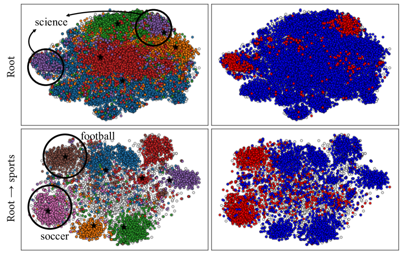
Figure 3. The embedding space of TaxoCom, which finds multiple sub-topic term clusters (Left) and discriminates between known-topic and novel-topic terms, respectively colored in blue and red (Right). Best viewed in color.

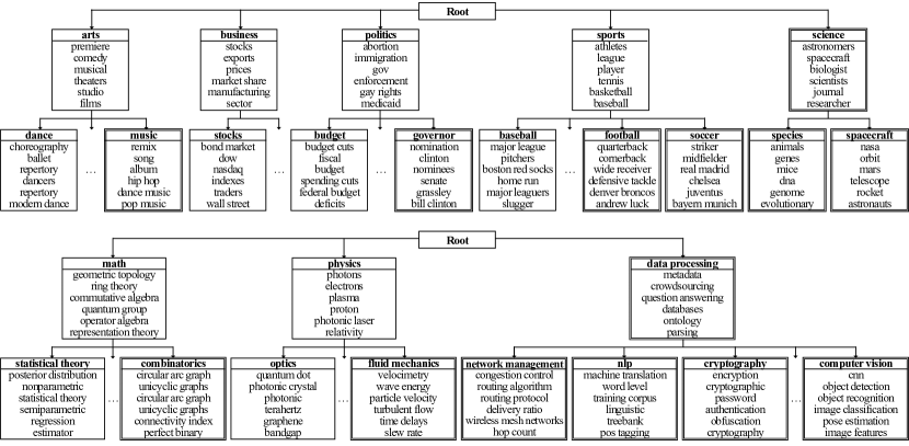
Figure 4. The output topic taxonomy of TaxoCom, where $\mathcal{H}_{c}$ is given as the initial topic hierarchy. Double-lined boxes represent the newly inserted topic nodes. Dataset: NYT (Upper) and arXiv (Lower).

5.2.3. Binary discrimination between known-topic and novel-topic documents

For each partial topic hierarchy, we provide an ablation analysis on the novelty detection performance of TaxoCom, to validate the effectiveness of the embedding techniques: local embedding (LE) and keyword-guided discriminative embedding (DE). Note that there do not exist term-level novelty labels, we instead use document-level novelty labels indicating whether a document belongs to one of the deleted ground-truth topic classes or not. In other words, we indirectly evaluate the capability of novel topic detection based on the topic assignment of documents, obtained by Equation (8). We consider precision, recall, and F1 score as the evaluation metrics. For a fair comparison, we select the optimal hyperparameter value $\beta\in\{1.5,2.0,2.5,3.0\}$ to determine the novelty threshold (in Equation (4)) of the ablated methods.

In Table 5, TaxoCom that adopts both LE and DE performs the best for distinguishing novel-topic documents from known-topic counterparts. Particularly, DE considerably improves the novelty detection performance, by collecting the given topic names from the sub-tree rooted at each node and utilizing them as the keywords for the topic, as discussed in Section 4.2.2. In summary, LE and DE optimize the embedding space further discriminative among known sub-topics, and it is helpful to enhance the binary discrimination between known and novel sub-topics as well.

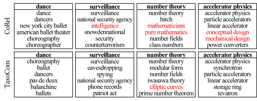
Figure 5. Topic terms retrieved by CoRel and TaxoCom.

5.3. Qualitative Analysis

5.3.1. Case study on topic taxonomy

We qualitatively examine the output taxonomy of TaxoCom. Figure 4 shows that TaxoCom expands the topic taxonomy while preserving the high-level design of the given topic hierarchy $\mathcal{H}_{c}$. To be specific, in case of NYT, it successfully identifies not only the first-level missing topic science but also the second-level ones including music, football, and soccer. We observe that several center terms of novel topic nodes do not exactly match with the ground-truth topic names, such as spacecraft-cosmos (NYT), data processing-computer science (arXiv), and fluid mechanics-fluid dynamics (arXiv). Nevertheless, it is obvious that they represent the same conceptual topic of some documents in the text corpus, in light of the terms assigned to them.

Furthermore, we compare the topic nodes (and their anchor terms) identified by TaxoCom and CoRel. In Figure 5, several topic terms of CoRel are too general to belong to the topic (marked in red), whereas TaxoCom selectively filters the topic-relevant terms by taking advantage of topic sub-corpus. In Table 6, CoRel often finds redundant topics semantically overlapped with a known sub-topic (✂), or just novel entities in the “is-a” relation rather than a topic class of documents in the corpus ($\operatorname*{\text{\raisebox{1.07639pt}{\scalebox{0.8}{$\bigotimes$}}}}$). Especially, CoRel fails to find any of the first-level missing topics due to the lack of given “is-a” relations. In contrast, TaxoCom effectively completes the latent topic structure of the text corpus by discovering novel topics that semantically deviate from the known topics.

Table 6. Novel sub-topics found by CoRel and TaxoCom.

Given $\mathbf{\bm{\mathcal{H}^{0}}}$		Topic	Identified Novel Sub-topics
			CoRel	TaxoCom
NYT	$\mathcal{H}_{a}$	root	-	arts
	$\mathcal{H}_{b}$	sports	baseball, softball($\operatorname*{\text{\raisebox{1.07639pt}{\scalebox{0.8}{$\bigotimes$}}}}$), squash($\operatorname*{\text{\raisebox{1.07639pt}{\scalebox{0.8}{$\bigotimes$}}}}$), wrestling($\operatorname*{\text{\raisebox{1.07639pt}{\scalebox{0.8}{$\bigotimes$}}}}$), …	baseball, hockey
	$\mathcal{H}_{c}$	arts	jazz, hip hop, acting(✂), animation($\operatorname*{\text{\raisebox{1.07639pt}{\scalebox{0.8}{$\bigotimes$}}}}$), ballet(✂), …	music
arXiv	$\mathcal{H}_{a}$	root	-	natural sciences
	$\mathcal{H}_{b}$	computer science	object detection, authentication(✂), database systems(✂), …	code construction, game, object recognition, parallel computing
	$\mathcal{H}_{c}$	physics	astrophysics(✂), general relativity(✂), particle physics(✂), …	atomic theory, fluid mechanics, electromagnetism(✂)

5.3.2. Visualization of discriminative embedding space

We also visualize our spherical embedding space for the NYT dataset, when $\mathcal{H}_{c}$ is given as the partial topic hierarchy. Figure 3 shows the embedding space plotted by t-SNE (Van der Maaten and Hinton, 2008) for (i) the root node and (ii) the sports node. In the left figures, the anchor terms assigned in multiple sub-topics are marked in different colors, while each center term and the non-anchor terms are plotted as black asterisks and white circles, respectively. We annotate the center term of the novel clusters that correspond to the novel topic nodes (i.e., science, football, and soccer) presented in Section 5.3.1. On the other hand, the right figures illustrate the binary discrimination between known-topic and novel-topic terms, determined based on the novelty score (Equation (4)). Our confidence-based novelty score is effective to detect novel-topic terms (and their dense clusters) clearly distinguishable from known-topic terms in the embedding space.

6. Conclusion

This paper studies a new problem, named topic taxonomy completion, which aims to complete the topic taxonomy initiated with a user-provided partial hierarchy. The proposed TaxoCom framework performs the hierarchical discovery of novel sub-topic clusters; it employs the text embedding and clustering tailored for effective discrimination between known sub-topics and novel sub-topics. The extensive experiments show that TaxoCom successfully outputs the high-quality topic taxonomy which accurately matches with the ground-truth topic hierarchy.

In future work, we would like to enhance the center term of novel topic nodes so that it can best summarize the high-level concepts of its sub-topic clusters. To this end, it would be interesting to (i) incorporate relation extraction techniques and (ii) employ a pre-trained language model; this could be a bridge technique between an entity taxonomy and a topic taxonomy, with a comprehensive understanding of entities, relations, documents, and topics.

Appendix A Supplementary Material

A.1. Pseudo-code of TaxoCom

Algorithm 1 describes the overall process of our framework for topic taxonomy completion. Starting from the root node (Line 2), TaxoCom recursively performs text embedding and clustering for each topic node (Lines 5 and 6) to find out multiple sub-topic term clusters. Based on the clustering result, it expands the current topic taxonomy by inserting novel sub-topic nodes (Line 8). In the end, TaxoCom outputs the complete topic taxonomy (Line 10).

1

Input: An input text corpus $\mathcal{D}$ with its term set $\mathcal{T}$, and a partial topic hierarchy $\mathcal{H}^{0}$

2

3 $\mathcal{H}\leftarrow\mathcal{H}^{0}$

4 $q\leftarrow queue([(\mathcal{H}^{0}.rootNode,\mathcal{T},\mathcal{D})])$

5 while $not$ $q.isEmpty()$ do

       $(c,\mathcal{T}_{c},\mathcal{D}_{c})\leftarrow q.pop()$

        $\triangleright$ Current node

       $\mathcal{E}_{c}\leftarrow$ Embedding($\mathcal{T}_{c},\mathcal{D}_{c};\mathcal{H}$)

        $\triangleright$ Section 4.2

       $\mathcal{R}_{c}\leftarrow$ Clustering($\mathcal{E}_{c},\mathcal{T}_{c},\mathcal{D}_{c};\mathcal{H}$)

        $\triangleright$ Section 4.3

6       for $(s,\mathcal{T}_{s},\mathcal{D}_{s})\in\mathcal{R}_{c}$ do

7             $\mathcal{H}.updateChildNodes(c,(s,\mathcal{T}_{s},\mathcal{D}_{s}))$

8             $q.push((s,\mathcal{T}_{s},\mathcal{D}_{s}))$

9            

10      

11return $\mathcal{H}$

Algorithm 1 The overall process of TaxoCom.

A.2. Implementation Details

We implement the main recursive process (Section 4.1) and the novelty adaptive clustering (Section 4.3) by using Python, and the locally discriminative embedding (Section 4.2) is written in C for efficient optimization based on multi-threaded parallel computation. For the other baselines, we employ the official author codes of hLDA , TaxoGen , JoSH , and CoRel .

For novelty adaptive clustering of TaxoCom, we set $\beta=1.5,3.0$ (for the first-level and second-level topic nodes, respectively) in the novelty threshold $\tau_{nov}$ (Equation (4)), and the significance threshold $\tau_{sig}=0.3$ (Equation (9)), without further tuning for each dataset or initial topic hierarchy. For locally discriminative embedding of TaxoCom, we set the margin $m=0.3$ (Equation (3)), and the number of neighbor terms $M=100$ (Section 4.2.1) to retrieve the sub-corpus which are used for tuning the embedding space, i.e., top-$100$ closest term of each center term.

For all the embedding-based methods (i.e., TaxoGen, JoSH, CoRel, and TaxoCom) that optimize the Euclidean space or spherical space, we fix the number of negative terms (for each positive term pair) to 2 during the optimization. For hLDA, we set (i) the smoothing parameter over document-topic distributions $\alpha=0.1$, (ii) the concentration parameter in the Chinese Restaurant Process $\gamma=1.0$, and (iii) the smoothing parameter over topic-word distributions $\eta=1.0$. For TaxoGen, we follow the parameter setting provided by (Zhang et al., 2018); i.e., the number of child nodes is set to 5.

A.3. Constructed Topic Taxonomy

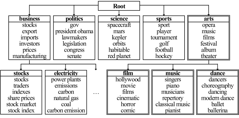
(a) Dataset: NYT

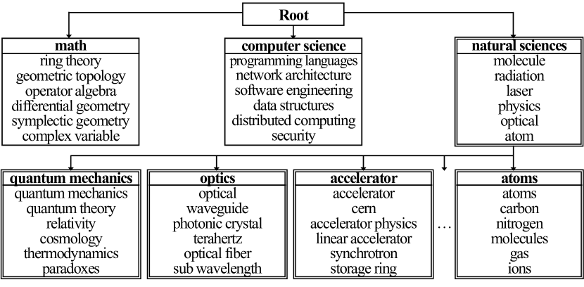
(b) Dataset: arXiv

Figure 6. The output taxonomy of TaxoCom, where $\mathcal{H}_{a}$ is given as the initial topic hierarchy. Double-lined boxes represent the novel topic nodes.

Figures 6 and 7 show the topic taxonomies generated by TaxoCom, where $\mathcal{H}_{a}$ and $\mathcal{H}_{b}$ are given as the initial topic hierarchy, respetively. The center terms (i.e., topic names) and topic terms are presented without any post-processing such as manual filtering or selection that requires human labor. Due to the space limit, the figures omit most of the second-level known topic nodes (i.e., the topics already included in $\mathcal{H}_{a}$ or $\mathcal{H}_{b}$), rather focus on newly inserted novel topic nodes. Note that the initial topic hierarchies are generated by random node drop of the ground-truth topic hierarchy: a single first-level topic (in case of $\mathcal{H}_{a}$) and a portion of second-level topics (in case of $\mathcal{H}_{b}$) is deleted, as listed in Table 2.

We can observe that TaxoCom effectively detects the deleted topic nodes and places them in the right position within the topic taxonomy. In other words, the output taxonomies more completely cover the topic structure of each dataset, compared to the initial topic hierarchy, $\mathcal{H}_{a}$ or $\mathcal{H}_{b}$. The recursive clustering process of TaxoCom implicitly forces the hierarchical semantic relationship of parent-child node pairs, while clearly distinguishing novel sub-topic clusters from known sub-topic clusters based on the score of how confidently each term belongs to one of the known sub-topics (Equation 4). As discussed in Section 5.3.1, some center terms of identified novel topic nodes do not match with the ground-truth topic names. In spite of the minor mismatch, we can easily figure out the one-to-one mapping from the novel topics to the deleted ground-truth topics; for example, films-movies, stock market-stocks, insurer-insurance (NYT), and natural sciences-physics, accelerator-accelerator physics, atoms-atomic physics (arXiv).

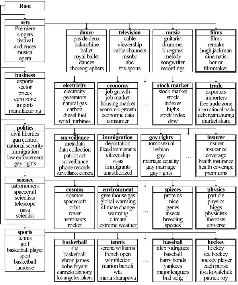
(a) Dataset: NYT

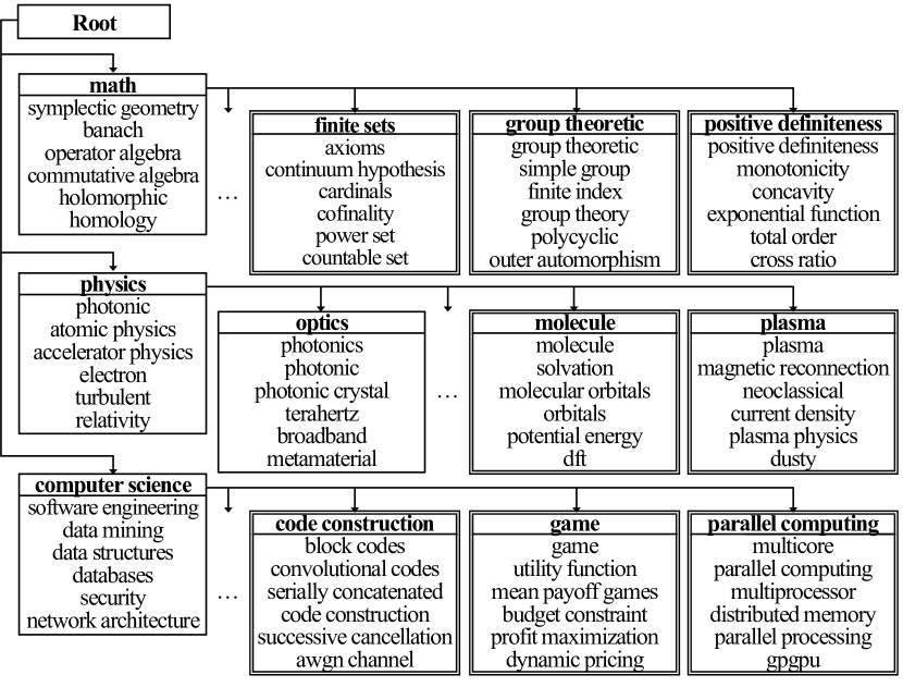
(b) Dataset: arXiv

Figure 7. The output taxonomy of TaxoCom, where $\mathcal{H}_{b}$ is given as the initial topic hierarchy. Double-lined boxes represent the novel topic nodes.