A Mock Catalog of Gravitationally Lensed Quasars for the LSST Survey

Abstract

We present a mock catalog of gravitationally lensed quasars at $z_{\text{qso}}<7.5$ with simulated images for the Rubin Observatory Legacy Survey of Space and Time (LSST). We adopt recent measurements of quasar luminosity functions to model the quasar population, and use the CosmoDC2 mock galaxy catalog to model the deflector galaxies, which successfully reproduces the observed galaxy velocity dispersion functions up to $z_{d}\sim 1.5$. The mock catalog is highly complete for lensed quasars with Einstein radius $\theta_{E}>0\farcs 07$ and quasar absolute magnitude $M_{i}<-20$. We estimate that there are $\sim 10^{3}$ lensed quasars discoverable in current imaging surveys, and LSST will increase this number to $\sim 2.4\times 10^{3}$. Most of the lensed quasars have image separation $\Delta\theta>0\farcs 5$, which will at least be marginally resolved in LSST images with seeing of $\sim 0\farcs 7$. There will be $\sim 200$ quadruply-lensed quasars discoverable in the LSST. The fraction of quad lenses among all discoverable lensed quasars is about $\sim 10\%-15\%$, and this fraction decreases with survey depth. This mock catalog shows a large diversity in the observational features of lensed quasars, in terms of lensing separation and quasar-to-deflector flux ratio. We discuss possible strategies for a complete search of lensed quasars in the LSST era.

1 Introduction

Gravitationally lensed quasars are valuable objects which enable a variety of unique studies in extragalactic astronomy. Examples include high-resolution observations of quasar host galaxies (e.g., Paraficz et al., 2018), studies of the dark matter profile and the circumgalactic medium of the foreground deflector galaxy (e.g., Gilman et al., 2020; Cashman et al., 2021), measuring the accretion disk size of background quasars (e.g., Cornachione & Morgan, 2020), and constraining key cosmological parameters such as the Hubble constant (e.g., Suyu et al., 2017). High-redshift lensed quasars are especially interesting, as they also probe the faint quasar population that are inaccessible without lensing magnification (e.g., McGreer et al., 2010; Yang et al., 2019; Yue et al., 2021b).

Despite their usefulness, gravitationally lensed quasars are rare, with about 120 of them discovered prior to 2015 (e.g., Inada et al., 2012). In the last few years, many searches for lensed quasar have been carried out utilizing recent wide-area imaging surveys, and have nearly doubled the sample size of lensed quasars (e.g., More et al., 2016; Lemon et al., 2018, 2019, 2020; Agnello et al., 2018; Treu et al., 2018; Spiniello et al., 2018; Jaelani et al., 2021). These searches have utilized effective candidate selection strategies for lensed quasars, based on their observed features like colors, morphologies and variabilities. In the near future, the Rubin Observatory Legacy Survey of Space and Time (LSST, Ivezić et al., 2019) will deliver deep, multi-band and multi-epoch imaging with sub-arcsec spatial resolution in a wide sky area, making it promising to build a large sample of lensed quasars in the next decade.

As the commissioning of LSST is approaching, there is a need to investigate the expected outputs of future surveys for lensed quasars, and to design a complete and efficient candidate selection strategy with LSST data. Mock catalogs and simulated observations are powerful tools to accomplish these tasks. In Oguri & Marshall (2010) (hereafter OM10), the authors present a mock catalog of lensed quasars, and discuss the number of lensed quasars that can be found in a number of surveys. Agnello et al. (2015) further generate simulated observations for the mock lensing systems using the properties of real galaxies and quasars from various of sky surveys. The simulated observations, as well as the candidate selection techniques developed based on it, have been proven to be effective in many lensed quasar searches (e.g., Agnello et al., 2018; Spiniello et al., 2018; Lemon et al., 2020).

However, the mock catalog in OM10 and the simulated observations have a few limitations. First, the OM10 mock catalog is based on early measurements of quasar luminosity functions (QLFs) and galaxy velocity dispersion functions (VDFs), while recent observations have provided more accurate measurements of the quasar and galaxy populations, especially at high redshifts. Second, the OM10 catalog only includes quasars at $z_{\text{qso}}<5.5$, while the depth and wavelength coverage of LSST will allow finding lensed quasars at redshift $z\gtrsim 7$. In addition, the simulated observations in Agnello et al. (2015) were largely based on wide-area sky surveys like the Sloan Digital Sky Survey (SDSS, York et al., 2000) and the Wide-field Infrared Survey Explorer (WISE, Wright et al., 2010), which are usually not deep enough to characterize faint galaxies at relatively high redshift. As such, the observed features of lensed quasars with faint (and thus less massive) deflector galaxies are not well-represented.

In this work, we present a new mock catalog of lensed quasars at $z_{\text{qso}}<7.5$ with simulated spectral energy distributions (SEDs) and LSST images, extending previous studies to higher quasar redshifts and smaller deflector galaxy masses. We use updated QLFs and VDFs to ensure accurate modeling of the lensed quasar population. This mock catalog predicts the number of discoverable lensed quasars in current and next-generation sky surveys, and can serve as training and testing sets in future searches for lensed quasars. This paper is organized as follows. We describe the method of generating the mock catalog in Section 2. Section 3 describes the predicted statistics of lensed quasars. Section 4 discusses some systematic uncertainties of the mock catalog and investigate possible strategies for future lensed quasar searches. We summarize in Section 5. Throughout this paper we use a flat Lambda cold dark matter ($\Lambda$CDM) cosmology with $H_{0}=70\text{ km s}^{-1}\text{ kpc}^{-1}$ and $\Omega_{M}=0.3$.

2 Mock Catalog Generation

In this section, we describe the method we use to generate the mock catalog, including simulations of the quasar population and the deflector galaxy population, as well as the matching and lensing algorithm. Figure 1 shows the flow chart of these processes.

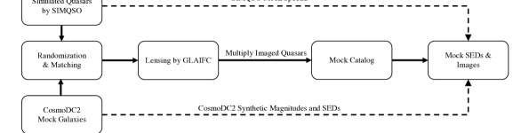
Figure 1: The flowchart of lensed quasar mock catalog generation process.

2.1 Deflector Population

We use the CosmoDC2 mock galaxy catalog (Korytov et al., 2019) to model the deflector galaxies. CosmoDC2 is a synthetic galaxy catalog that covers an area of 440 deg² out to a redshift of $z=3$. CosmoDC2 first identifies dark matter halos in the $N-$body simulation Outer Rim (Heitmann et al., 2019), and assigns simulated galaxies from the UniverseMachine (Behroozi et al., 2019) to the dark matter halos. The algorithm is tuned to match the observed stellar mass versus star formation rate $(M_{*},\text{SFR})$ distributions of galaxies. CosmoDC2 then assigns various of properties to the mock galaxies, including stellar masses, optical-to-near infrared (NIR) SEDs, half-light radii and ellipticities, using empirical relations or simulated galaxy spectra library. Korytov et al. (2019) shows that the mock catalog reproduces the observed colors and number counts of galaxies at a wide range of redshifts. The large area of CosmoDC2 catalog ensures a small statistical error of the simulated lens sample, and the galaxy properties provides all the information needed to generate mock observations of lensing systems.

We use singular isothermal ellipsoids (SIE, e.g., Kormann et al., 1994) to model the lensing potential of the deflector galaxies. An SIE lens is parameterized by its ellipticity, $e=1-q$ where $q$ is the axis ratio, and its Einstein radius,

$$\theta_{E}=4\pi\left(\frac{\sigma}{c}\right)^{2}\frac{D_{\text{ds}}}{D_{\text{s}}}$$ (1)

where $\sigma$ is the line-of-sight velocity dispersion of the galaxy, $D_{\text{s}}$ is the angular diameter distance from the observer to the source, and $D_{\text{ds}}$ is the angular diameter distance from the deflector to the source.

We estimate the velocity dispersion of a galaxy using its stellar mass. Specifically, we convert stellar masses to dynamical masses using a stellar-to-dynamical mass ratio, and calculate the velocity dispersion by applying the virial theorem (e.g., Cappellari et al., 2006):

$$\sigma=\sqrt{\frac{GM_{\text{dyn}}}{KR_{e}}}$$ (2)

We adopt $M_{*}/M_{\text{dyn}}=0.557$, which gives a good description for galaxies in a wide mass $(100\text{ km s}^{-1}<\sigma<300\text{ km s}^{-1})$ and redshift $(0<z<1)$ range (e.g., Bezanson et al., 2011, 2012). Since early-type galaxies dominates the deflector population in galaxy-scale lenses (e.g., Oguri, 2006; Inada et al., 2012), we adopt the typical scaling factor $K=6$ for early-type galaxies (e.g., Beifiori et al., 2014; Nigoche-Netro et al., 2016). We do not use the Sérsic-index-dependent scaling factor as suggested in, e.g., Bertin et al. (2002), as CosmoDC2 uses a bulge + disk composition to describe the galaxy morphology instead of a Sérsic profile.

Figure 2 compares the derived VDF of the CosmoDC2 mock galaxy catalog with the observed galaxy VDF. The local VDF has been accurately measured spectroscopically (e.g., Choi et al., 2007). We find that the VDF of the CosmoDC2 catalog at $z<0.1$ is fully consistent with the recent spectroscopic measurements (Sohn et al., 2017; Hasan & Crocker, 2019). At higher redshifts, it is challenging to measure the velocity dispersion of a large galaxy sample and thus the VDF spectroscopically. The right panel of Figure 2 compares the CosmoDC2 catalog VDF with the observed VDF at $z<1.5$ from Bezanson et al. (2012), who measure the dynamical mass of galaxies in the COSMOS and UDF fields using photometric data. The CosmoDC2 catalog is also in good agreement with the observed values except at the low-mass end at $z>0.6$, which can be due to incompleteness of the galaxy sample in the observations. Figure 2 suggests that our method successfully reproduces the observed VDF at least at $z<1.5$.

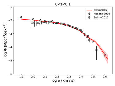
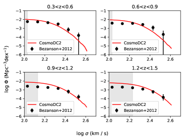
Figure 2: The comparison between the derived VDFs of the CosmoDC2 catalog and the observed VDF at $z<1.5$. Left: The local $(z<0.1)$ VDF. The VDF of the CosmoDC2 catalog accurately matches the spectroscopically measured VDF in Sohn et al. (2017) and Hasan & Crocker (2019). Right: The VDF at $0.3<z<1.5$. The gray area marks the region where Bezanson et al. (2012) suggest that their galaxy sample has a low completeness. The CosmoDC2 VDF is in good agreement with the observed VDF up to $z=1.5$. At the less massive end, the CosmoDC2 catalog gives a higher number density than the observation, which can be explained by the incompleteness of the observed galaxy sample.

In this work, we only include galaxies with $\sigma>50\text{ km s}^{-1}$, which corresponds to an Einstein radius limit of $\theta_{E,\text{lim}}=4\pi(\sigma_{\text{lim}}/c)^{2}=0\farcs 072$. Lensing systems with smaller $\theta_{E}$ are difficult to identify even with space telescopes like the Hubble Space Telescope (HST).

We notice that the observed $M_{*}-\sigma$ relation have significant scatters, which can be partly explained by the effect of galaxy sizes $(R_{e})$. The observed scatter of Equation 2 is $\sim 0.02$dex for the velocity dispersion (e.g., Auger et al., 2010). This small scatter have little influence on the galaxy VDF, and is not considered in this work.

In addition to the deflector galaxy, we add an external shear and convergence to each lensing system. We use the CosmoDC2 catalog to estimate the redshift evolution of external shears and convergences. Specifically, we divide the mock galaxy catalog into redshift bins with $\Delta z=0.01$, then fit the distribution of external convergences $(\kappa)$ and the two components of the external shear $(\gamma_{1},\gamma_{2})$ in each redshift bin as normal distributions centered at zero. For both $\kappa$ and $\gamma$, the best-fit standard deviation can be well-described by a linear function of $\log(1+z)$:

$$\begin{split}\sigma_{\kappa}&=0.057\times\log(1+z)-0.001\\ \sigma_{(\gamma_{1}\text{ or }\gamma_{2})}&=0.040\times\log(1+z)-0.001\end{split}$$ (3)

For each lensing system, we use the best-fit normal distribution to generate a random set of $(\kappa,\gamma_{1},\gamma_{2})$ values.

Note that the convergence and shears in the CosmoDC2 catalog have some limitations. Specifically, the convergence and shears from ray-tracing simulations depend on the resolution (i.e., the smoothing scale) of the density field, especially at small scales (e.g., Hilbert et al., 2009). To perform the ray-tracing simulation, CosmoDC2 divides the mass particles from the cosmological simulation into discrete shells and estimates the surface mass density of each shell on a HEALPix grid with Nside=4096, which corresponds to a resolution of 0.5 arcminutes on the sky. Korytov et al. (2019) compares the cosmic shear power spectrum of the CosmoDC2 catalog and theoretical predictions, showing that the difference is negligible at $\ell<1000$ and is $\lesssim 10\%$ at $\ell\sim 4000$. As the values of $\kappa$ and $\gamma$ are small (Equation 3), this systematic uncertainty has effectively no impact on the number of lensed quasars.

2.2 Quasar Population

We simulate quasars at $z<7.5$ using python code SIMQSO (McGreer et al., 2013). SIMQSO generates mock catalogs of quasars by randomly sampling the absolute magnitude and the redshift of quasars according to the input QLF. For each simulated quasar, SIMQSO generates a mock spectrum which includes a broken power-law continuum and a number of emission line components, and sets a random sightline to model the intergalactic medium (IGM) absorption based on observed IGM models. We use the default continuum, emission line and IGM parameters in SIMQSO which has been shown to successfully reproduce the observed quasar color distribution (e.g., Ross et al., 2013) and has been widely used to estimate the completeness of quasar surveys (e.g., Jiang et al., 2016; Yang et al., 2016; McGreer et al., 2018; Wang et al., 2019).

We use a double power-law to describe the QLF:

$$\Phi(M,z)=\frac{\Phi_{*}}{10^{0.4(M-M^{*})(\alpha+1)}+10^{0.4(M-M^{*})(\beta+1)}}$$ (4)

where $\alpha$ and $\beta$ are faint and bright end slopes of the QLF, $M^{*}$ is the break absolute magnitude and $\Phi_{*}$ is the normalization. Specifically, the QLF we adopt at different redshifts are as follows:

1. At $0<z<3.5$, we adopt the pure luminosity evolution (PLE, for $z<2.2$) and the luminosity evolution and density evolution (LEDE, for $2.2<z<3.5$) model from Ross et al. (2013). We use the relations in the Appendix B of Ross et al. (2013) to convert the absolute magnitudes to $M_{\text{1450}}$, i.e., the absolute magnitude at rest-frame 1450Å.

2. At $3.5<z<7.5$, we compile a number of QLFs at different redshifts from the literature. These QLFs are summarized in Table 1. At $3.5<z<6.7$, we use linear interpolation to obtain the QLF parameters at a certain redshift. At $z>6.7$, we keep $\alpha,\beta$ and $M^{*}$ fixed to the $z=6.7$ value, and apply a density evolution of $\log\Phi_{*}(z)=\log\Phi_{*}(z=6.7)-0.78\times(z-6.7)$, following Wang et al. (2019).

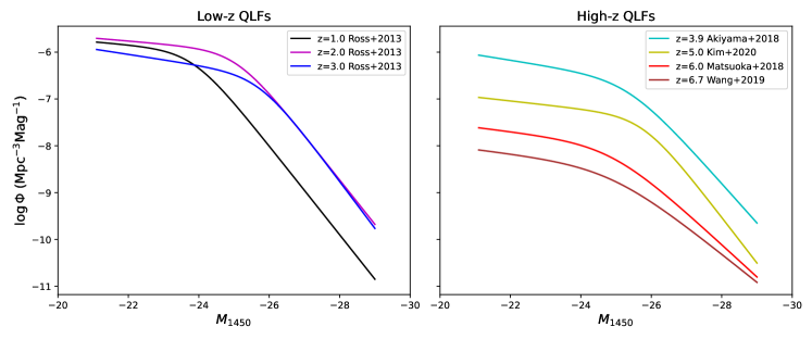
Figure 3: QLFs adopted by this work. We use the QLF from Ross et al. (2013) to model quasars at $z<3.5$, and compile a number of literature to construct the QLF at $z>3.5$ (see text for details). Left: The Ross et al. (2013) QLFs. Right: The high-redshift QLFs we use from the literature. At $z\gtrsim 4$, the values of $M^{*},\alpha$ and $\beta$ do not show strong redshift evolution, suggesting that a linear interpolation between the redshifts is adequate.

Figure 3 shows the QLF used in this work at different redshifts. Both Table 1 and the right panel of Figure 3 suggest a subtle redshift evolution of $M^{*},\alpha$ and $\beta$ at high redshift. In addition, a linear interpolation of $\log\Phi_{*}$ is equivalent to an exponential redshift evolution of $\Phi_{*}$, which has been shown to well-describe the number density of high-redshift quasars (e.g., Jiang et al., 2016; McGreer et al., 2018; Wang et al., 2019). Using linear interpolations between redshifts is thus sufficient to accurately capture the evolution of QLFs at high redshift.

Following the Active Galactic Nuclei (AGN) chapter in the LSST science book (LSST Science Collaboration et al., 2009), we only include quasars with $M_{i}<-20$ in our simulated quasar sample, which is equivalent to $M_{1450}<-19.1$ according to the relation in Ross et al. (2013). For faint AGN below this flux limit, host galaxies start to dominate their emissions. These objects require a survey strategy that is different from classical quasars and is out of the scope of this paper.

The area of the CosmoDC2 catalog is 440 deg², which is $1.067\%$ of the whole sky. To make the simulated lens catalog equivalent to an all-sky catalog, we scale the QLF by a factor of $2\%/1.067\%=1.874$, so that the number of expected lensed quasars in the CosmoDC2 field equals to $1/50$ of the sky. By running 50 random realizations (see Section 2.3), we can obtain a mock catalog that is equivalent to the all-sky area.

Table 1: QLF Parameters from the Literature

Redshift	$\log{\Phi_{*}}$	$M^{*}$	$\alpha$	$\beta$
	$(\text{Mpc}^{-3}\text{mag}^{-1})$	(mag)
$0.1<z<2.2$	$-5.96^{+0.02}_{-0.06}$	$-21.364^{+0.05}_{-0.11}-2.5\times(1.241^{+0.010}_{-0.028}z-0.249^{+0.006}_{-0.017}z^{2})$	$-1.16^{+0.02}_{-0.04}$	$-3.37^{+0.03}_{-0.05}$
$2.2<z<3.5$	$-5.83^{+0.15}_{-0.25}-0.689^{+0.021}_{-0.027}\times(z-2.2)$	$-25.00^{+0.34}_{-0.24}-0.809^{+0.033}_{-0.166}\times(z-2.2)$	$-1.31^{+0.52}_{-0.19}$	$-3.45^{+0.35}_{-0.21}$
$z=3.9$	$-6.58\pm 0.01$	$-25.36\pm 0.13$	$-1.30\pm 0.05$	$-3.11\pm 0.07$
$z=5.0$	$-7.36^{+0.56}_{-0.81}$	$-25.78^{+1.35}_{-1.10}$	$-1.21^{+1.36}_{-0.64}$	$-3.44^{+0.66}_{-0.84}$
$z=6.0$	$-7.96^{+0.28}_{-0.42}$	$-24.90^{+0.75}_{-0.90}$	$-1.23^{+0.44}_{-0.34}$	$-2.73^{+0.23}_{-0.31}$
$z=6.7$	$-8.43\pm 0.23$	$[-24.90]$	$[-1.23]$	$-2.51\pm 0.39$

Note. — The parameters are defined in Equation 4. Absolute magnitudes in this table are $M_{1450}$. The square brakets marks quantities that are fixed when fitting the QLFs. Specifically, Wang et al. (2019) only measures the bright end of $z\sim 6.7$ QLF, and we fit the double power-law by fixing the $M^{*}$ and $\alpha$ values to that of Matsuoka et al. (2018). For $3.5<z<6.7$, we perform linear interpolation to obtain QLF model parameters. For $z>6.7$, we assume a pure density evolution of $\log\Phi_{*}(z)=\log\Phi_{*}(z=6.7)-0.78\times(z-6.7)$, following Wang et al. (2019).

2.3 Lensing Pipeline

After producing the mock deflector galaxies and the simulated background quasars, we generate one realization of the mock lens catalog as follows. We first assign random positions in the CosmoDC2 field to the simulated quasars, and assign random position angles to the mock galaxies. Then, for each galaxy, we identify all quasars that have distances to the galaxy smaller than $5\theta_{E,max}$, where $\theta_{E,max}=4\pi(\sigma/c)^{2}$ is the maximum possible Einstein radius for the deflector galaxy. For each matched galaxy-quasar pair, we assign a random external convergence and a random external shear according to the best-fit probabilistic distribution described in Section 2.1, and use GLAFIC (Oguri, 2010) to model the lensing configuration. GLAFIC is a software that provides fast and flexible lensing analysis for a variety of deflector mass and source emission models. We then select multiply-imaged quasars into the mock lens catalog.

We run 50 random realizations to generate a mock lens catalog that is equivalent to the all-sky area. For quasars at $z>5$, due to their low number density, we run 1,000 realizations (i.e., $20\times$ all-sky area) to reduce the Poisson noise.

2.4 Broad-Band Photometry and Mock Images

We calculate the magnitdues of the simulated lensed quasars in the LSST $ugrizy$, UKIDSS $JHK$ (Lawrence et al., 2007), and WISE W1, W2 bands. We use the simulated spectra generated by SIMQSO to calculate the synthetic magnitudes of quasars. For deflector galaxies, CosmoDC2 provides the synthetic LSST $ugrizy$ magnitudes and 30 top-hat SED points in the wavelength range $1000\text{\AA}<\lambda<20000\text{\AA}$. We directly adopt the synthetic $ugrizy$ magnitudes from the CosmoDC2 catalog, and estimate the $JHK$ and W1, W2 magnitudes using the SED. Specifically, the SED covers $J$ and $H$ at all redshifts, and we linearly interpolate the SED points to build a spectra and calculate the magnitudes. At low redshifts, the SED does not cover the wavelengths of $K$, W1 and/or W2. In this case, we fit the SED using the galaxy templates from Brown et al. (2014), and use the best-fit template to estimate the magnitude in that filter.

To further explore how survey strategies work for real data, we generate simulated LSST images in $ugrizy$ bands for the mock lensed quasars. We use point sources to describe the lensed images of the background quasar, and use a bulge (de Vaucouleurs) + disk (exponential) two-component model to describe the foreground galaxy. CosmoDC2 provides the radius and the SED of both components for each galaxy. We then generate mock images using galfit (Peng et al., 2002) for each lensing system. Specifically, the images are created as follows:

1. The Point Spread Function (PSF): The PSF of each image is modeled as an 2-D Gaussian profile. The full-width half maximum (FWHM) is drawn from a normal distribution with a standard deviation $\sigma_{\text{FWHM}}=0.02\times mean$, where $mean$ is the mean PSF size of the corresponding filter. The axis ratio is uniformly drawn in $[0.95,1]$, and the position angle is uniformly drawn from $[0,2\pi)$. This approach mimics the PSF variation in real observations.

2. Image Noises: We follow the methods in the LSST review paper (Ivezić et al., 2019, also see https://smtn-002.lsst.io/) to calculate the errors of image pixels. The random noise of an pixel consists of the background noise and the Poisson noise of the source flux. These noises are calculated based on Equation 5 in Ivezić et al. (2019).

Table 2 summarizes the mean PSF sizes and depths we used in the simulation. Figure 4 shows some examples of the SED and simulated LSST images of a mock lensed quasar, which exhibit a large diversity in observational features.

Table 2: PSF Size and Depth of the Mock LSST Images

Filter	$5-\sigma$ Depth	PSF FWHM
	(mag)	$(^{\prime\prime})$
$u$	26.1	0.81
$g$	27.4	0.77
$r$	27.5	0.73
$i$	26.8	0.71
$z$	26.1	0.69
$y$	24.9	0.68

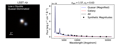
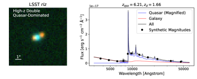
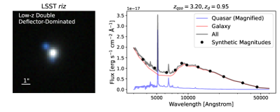
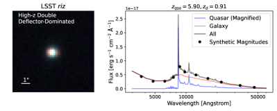
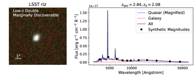
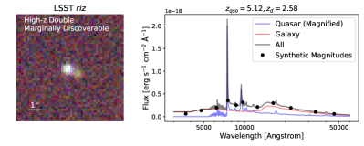
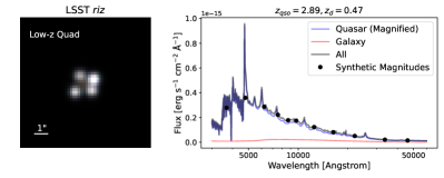
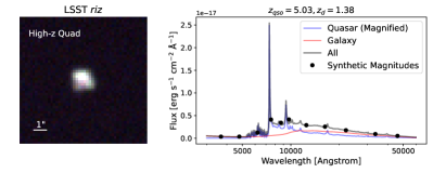
Figure 4: A gallery of mock lensed quasars. We show several typical cases for both the low-redshift and the high-redshift sample. The synthetic magnitudes are in LSST $ugrizy$, UKIDSS $JHK$, and WISE W1, W2 bands. The mock lensed quasars show a large diversity in observational features in magnitudes, colors, lensing separations, etc. It is worth noticing that (1) the deflector galaxy is always at the center of the image, and is usually blended with the fainter lensed image in doubly-lensed systems; (2) the low-redshift example of a “marginally discoverable” lens (third row, left) has a small lensing separation of $0\farcs 5$, and the high-redshift example (third row, right) has a marginally detectable fainter image (which is blended with the deflector galaxy). See section 3 for the definition of discoverable lenses.

The final data products are a mock catalog of lensed quasars and mock LSST images for each simulated lensed quasar. We provide a number of properties in the mock catalog, including the lensing configuration, the time delay of each lensed image, and the magnitudes of the quasar and the deflector. These properties are summarized in Table 3.

Table 3: Description of the columns in the mock catalog

Name	Format	Description
Quasar Parameters
qidx	int	The unique identifier of the mock quasar.
zq	float	The redshift of the mock quasar.
qra	float	The RA of the mock quasar, in degrees.
qdec	float	The Dec of the mock quasar, in degrees.
absMag	float	The absolute magnitude at rest-frame 1450Å $(M_{1450})$.
QSOMags	list of floats	The synthetic, unmagnified magnitudes of the mock quasar in LSST $ugrizy$, UKIDSS $JHK$ and WISE W1, W2.
Deflector Parameters
galaxy_id	int	The “galaxy_id” field of the mock galaxy in the CosmoDC2 catalog.
zg	float	The redshift of the mock galaxy.
gra	float	The RA of the mock galaxy, in degrees.
gdec	float	The Dec of the mock galaxy, in degrees.
rmaj	float	The semi-major axis of the galaxy, in arcsec.
rmin	float	The semi-minor axis of the galaxy, in arcsec.
pa_lens	float	The position angle of the galaxy (following GLAFIC conversion).
stellar_mass	float	The stellar mass in $M_{\odot}$.
sigma	float	The velocity dispersion, in km/s.
GalMags	list of floats	The synthetic total magnitudes of the deflector galaxy in LSST $ugrizy$, UKIDSS $JHK$ and WISE W1, W2.
shear_1, shear_2	float	The $x-$ and $y-$ components of the external shear.
convergence	float	The external convergence.
Lensing Configuration
Nimg	int	The number of lensed images.
image_x	list of floats	the x-coordinates of the lensed images, in arcsec (following GLAFIC conversion).
image_y	list of floats	the y-coordinates of the lensed images, in arcsec.
image_mu	list of floats	the magnification of the lensed images.
image_dt	list of floats	the time delay of the lensed images, in days.

3 Statistics of Lensed Quasars

Table 4: Predicted Number of Discoverable Lensed Quasars

Survey	Area	Filter	$5\sigma$ Depth	FWHM	$N_{\text{qso}}$	$N_{\text{lens}}$	$N_{\text{quad}}$
	$(\text{deg}^{2})$		(mag)	$(^{\prime\prime})$
PS1	$3\times 10^{4}$	$i$ or $z$	23.1 or 22.3	1.11 or 1.07	$4.8\times 10^{6}$	928	132
Legacy	$1.4\times 10^{4}$	$r$ or $z$	23.5 or 22.5	1.18 or 1.11	$2.6\times 10^{6}$	474	70
LSST	$2\times 10^{4}$	$i$ or $z$	26.8 or 26.1	0.71 or 0.69	$7.4\times 10^{6}$	2377	193
DES	$5\times 10^{3}$	$i$ or $z$	23.8 or 23.1	0.88 or 0.83	$1.0\times 10^{6}$	241	33
HSC	$1.4\times 10^{3}$	$i$ or $z$	26.4 or 25.5	0.56 or 0.63	$5.1\times 10^{5}$	165	14

Note. — See Section 3 for the criteria of a discoverable lensed quasar. We consider two filters for each survey, and a lensed quasar will be counted if it is discoverable in either band.

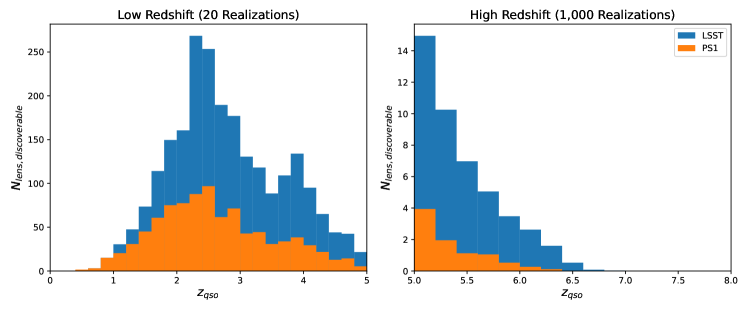
Figure 5: Predicted number of discoverable lensed quasars in LSST and PS1 survey, as a function of redshift. See Section 3 for the definition of a discoverable lensed quasar. Left: the low-redshift $(z_{\text{qso}}<5)$ sample. We run 50 realizations which is equivalent to an all-sky area, and scale the predicted number of discoverable lenses according to the survey area (listed in Table 4). There are $\sim 900$ discoverable lensed quasars in the PS1 survey, and LSST will increase this number to about $2.4\times 10^{3}$. Note that there is a bump at $z_{\text{qso}}\sim 4$ in lensed quasar numbers, where we switch from the low-redshift QLF to the high-redshift one. The faint-end values of the two QLFs are not fully consistent at this redshift. Right: the high-redshift $(z_{\text{qso}}>5)$ sample. We run 1,000 realizations to reduce the statistical error since the number density of high-redshift quasars is low. The mock catalog suggests that only a handful of lensed quasars at $z_{\text{qso}}>5$ are discoverable in current imaging surveys like PS1, and there will be $\sim 45$ discoverable in LSST. At $z\gtrsim 6.5$, there are effectively no discoverable lensed quasars even for LSST.

In this section we present the numbers of lensed quasars that are discoverable in various of imaging surveys. Following Oguri & Marshall (2010), we define a lensed quasar to be discoverable if: (1) it has a separation of $\Delta\theta>\frac{2}{3}\times\text{FWHM}$ and (2) has the second (for doubly-imaged lenses) or third (for quadruply-imaged lenses) brightest lensed image detectable in a $5\sigma$ level. Here, the separation of a lensed quasar is defined as the largest separation between any pairs of the lensed images. These criteria ensure that the lensing structure is at least marginally resolved.

Note that while lensed quasars that meet the critera above are in principle discoverable, in practice, their recovery faces a number of technical challenges. In real observations, the flux contribution of the lensing galaxy, low signal to noise ratios, and the presence of large number of both astrophysical and instrumental contaminants could result in significant challenges and low success rate in lensed quasar selection, especially for the marginally discoverable cases. As a result, most of the lensed quasars reported in recent surveys are bright ones with large separation (e.g., Lemon et al., 2020; Chan et al., 2020). A main application of this catalog is to facilitate development of selection algorithm to enable effective recoveries of these discoverable systems.

In Table 4, we list the predictions for a number of current and next-generation imaging surveys. As specific examples, Figure 5 shows the redshift distribution of discoverable lensed quasars in the PS1 survey and the LSST survey. Our mock catalog suggests that current sky surveys such as PS1 can in principle find $\sim 900$ of lensed quasars, and LSST will increase this number to $\sim 2.4\times 10^{3}$. Most of the lensed quasars have redshift $1.5<z_{\text{qso}}<3.5$, which is consistent with the statistics of the current sample of discovered lensed quasars. Due to the decline of the quasar number density, the numbers of discoverable lensed quasars drop quickly at $z_{\text{qso}}\gtrsim 4$. Figure 5 suggests that only a handful lensed quasars at $z_{\text{qso}}>5$ are discoverable in imaging surveys such as PS1, and there will be $\sim 45$ discoverable in LSST. There are effectively no discoverable lensed quasars at $z>7$ even in the LSST survey. We will discuss in more details the lensed fraction of $z\gtrsim 6$ quasars using both the mock catalog and analytical models in a subsequent paper (Yue et al., 2021a).

It is worth noticing that, even though LSST reaches more than three magnitude deeper than PS1, the number of total quasars and discoverable lensed quasars are only 1.5 and 2.6 times higher. This is due to the fact that we only include quasars with $M_{i}<-20$ in the catalog so that the AGNs are not host-dominated. LSST reaches significantly fainter flux level than this limit especially at low redshift.

Figure 6 shows the distribution of lensing separations of the mock lensed quasars. About $\sim 80\%~{}(50\%)$ of these lenses have separation larger than $0\farcs 5~{}(1\farcs 0)$. These numbers are consistent with the results in, e.g., Hilbert et al. (2008) and Collett (2015). A ground-based imaging survey with a PSF size of $\sim 0\farcs 7$ will be sufficient to make most of the lenses marginally resolved, which suggests that the bottleneck of lensed quasar surveys is the image depth rather than the PSF size.

We note that the predicted number of lensed quasars in this work is about two to three times lower than that of OM10, especially for deep surveys like HSC and LSST. The main reason is the difference in the simulated quasar sample; OM10 adopt a steeper QLF faint-end slope, and more importantly, they do not apply a cut in the absolute magnitude, while we only include quasars with $M_{i}<-20$. In addition, OM10 use a deflector VDF without redshift evolution, in contrast to the CosmoDC2 VDF which declines with redshift. In Section 3.1 we discuss in more details the difference between our mock catalog and that of OM10, where we show that the number of lensed quasars are consistent after taking the difference in QLFs and VDFs into account.

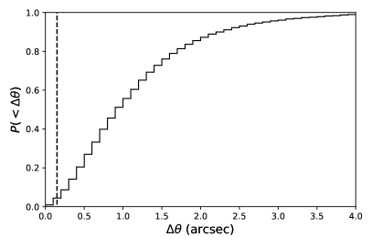
Figure 6: The distribution of the image separations of lensed quasars. The dashed line marks the limit above which the mock catalog is complete. About $\sim 50\%$ of the lensed quasars have separation $\Delta\theta>1^{\prime\prime}$, and $\sim 80\%$ of them have $\Delta\theta>0\farcs 5$.

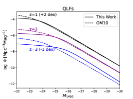
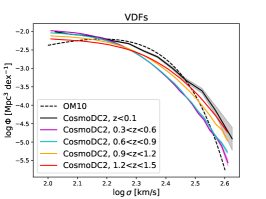
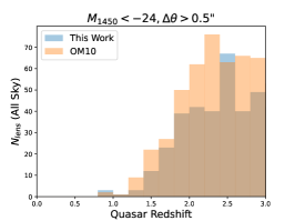
Figure 7: Comparison between this work and OM10. Left: the QLF adopted in this work and OM10. The two QLFs are nearly identical for quasars at $z\lesssim 2.5$ with $M_{1450}<-24$. Middle: The VDF adopted in this work and OM10. We show the CosmoDC2 VDF at $z<1.5$ which covers the majority of deflector galaxies for $z_{\text{qso}}\lesssim 2.5$. OM10 uses the local VDF in Choi et al. (2007) and assumes no redshift evolution. The local VDF of the CosmoDC2 catalog is close to the one used by OM10, and the OM10 VDF is slightly higher than the CosmoDC2 VDF at higher redshift. Right: the predicted number of lensed quasars at $z<3$. We only select lensed quasars with $\Delta\theta>0\farcs 5$ and $M_{1450}<-24$, at which the QLFs used by OM10 and this work are close to each other. Our mock catalog predicts slightly smaller numbers of lensed quasars than OM10 when only restricted to these parameter ranges, and the different can be fully explained by the adopted QLFs and VDFs (see text for details).

3.1 Comparison with the OM10 Mock Catalog

The mock catalog in OM10 and this work have a number of significant difference: (1) The two mock catalogs adopt different QLFs and VDFs. (2) We only include quasars with $M_{i}<-20$, while OM10 extend the quasar sample to as faint as $M_{i}\sim-18$. And (3) OM10 only include lensing systems with separation $\Delta\theta>0\farcs 5$, while our mock catalog have more compact lenses down to $\Delta\theta\sim 0\farcs 1$.

To perform meaningful comparisons, we select subsamples of the two mock catalogs that have $M_{1450}<-24$, $z_{\text{qso}}<3$ and $\Delta\theta>0\farcs 5$. In this redshift and magnitude range, the QLFs used in OM10 and this work are close to each other (Figure 7, left panel). We also compare the VDFs adopted in OM10 and this work in the middle panel of Figure 7. In short, OM10 adopt the local VDF from Choi et al. (2007) and assume no redshift evolution. This VDF is close to the CosmoDC2 catalog VDF at $z<0.1$, but it predicts higher number density than the CosmoDC2 VDF beyond the local universe. These differences can fully account for the predicted numbers of lensed quasars, shown in the right panel of Figure 7. After applying the luminosity, redshift and lensing separation cuts mentioned above, our mock catalog gives a slightly smaller number of lensed quasars compared to OM10. The main difference between the two mock catalogs appears at $z_{\text{qso}}\sim 2.2$, where the OM10 catalog has $\sim 30\%$ more lenses than this work. This can be explained by the difference in the VDFs at $z_{d}\gtrsim 0.3$, where the OM10 VDF is $\sim 0.3$ dex higher than the CosmoDC2 VDF.

The comparison suggests that our method of generating mock catalog is reliable, and illustrates the importance of using accurate and updated QLFs and VDFs. Another major difference between OM10 and this work is that we apply an absolute magnitude cut of $M_{i}<-20$ for quasars. This cut is used in the LSST science book, and the main motivation is that fainter AGNs have distinct observational features compared to normal type-I quasars. For these objects, host galaxy emissions start to dominate the SEDs and make their morphology extended. Modeling the host galaxy emission is out of the scope of this work, and we expect that these faint AGNs require a very different candidate selection strategy.

AGN variability offers a possible way of finding host-dominated lensed AGNs (e.g., Kochanek et al., 2006). OM10 presented the number of lensed quasars that are brighter than the 10$\sigma$ limits of yearly-stacked images for each sky survey, which can be identified via their variability. Variability analysis will be especially useful in the LSST survey, providing a critical supplement to image-based candidate selection methods.

3.2 Quadruply-Lensed Quasars and Time Delays

One important application of lensed quasars is to measure key cosmological parameters, especially the Hubble constant $H_{0}$. This relies on measuring the time delays between the lensed images of the background quasar. Compared to doubly-imaged ones, quadruply lensed quasars are preferred since they provide more time delays and give stronger constraints.

Table 4 gives the number of discoverable quadruply-lensed quasars in various sky surveys. Our mock catalog suggests that there are $\sim 200$ quadruply-lensed quasars discoverable in LSST. The impact of survey depth on the number of discoverable lenses is less significant for quads compared to doubly-lensed quasars, which is a result of magnification bias and the criteria of discoverable lenses (Section 3). In general, the fainter image in doubly-lensed systems has a low magnification and is often de-magnified $(\overline{\mu}=0.6)$, while the third brightest images in quad lenses have significantly higher magnifications $(\overline{\mu}=2.6)$. Given the luminosity limit of our quasar sample $(M_{i}<-20)$, most quadruply-lensed quasars are brighter than the LSST survey limit. Nonetheless, the image quality of LSST is still critical to the search of these bright quads, since the better depth and spatial resolution are essential for a high completeness and efficiency in the candidate selection.

Figure 8 further illustrates the number of discoverable quaduply lensed quasars as a function of survey depth. We assume an LSST-like PSF size of $0\farcs 7$ when counting the number of discoverable lenses, and normalize the numbers to the area of LSST. We also include the number of doubly-lensed quasars and unlensed quasars for comparison. Note that the magnitudes in Figure 8 correspond to the second brightest image for doubly-lensed quasars and the third brightest image for quadruply-lensed ones, in accordance with the definition of discoverable lensed quasars. At $m_{i}\lesssim 25$, about $\sim 10\%-15\%$ of the discoverable lensed quasars are quads. The magnification bias makes the fraction of quads decreases with survey depth, in agreement with the result in OM10. The number of quad lenses drops quickly at $m_{i}\gtrsim 26$, which is a result of the absolute magnitude cutoff.

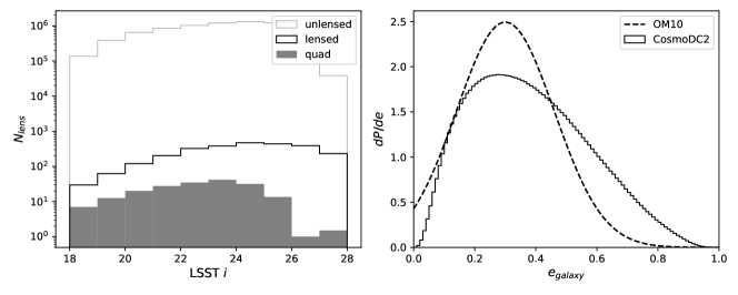
Figure 8: Left: The number of discoverable quadruply-lensed quasars as a function of survey depth. We also include doubly-lensed quasars and unlensed quasars for comparison. We use the LSST survey area and seeing condition when computing the numbers. The magnitudes correspond to the second brightest image for doubly lensed quasars, and the third brightest image for quad lenses. The fraction of quadruply lensed quasars among all lenses is $\sim 10\%-15\%$ at $m_{i}\lesssim 25$. This fraction drops quickly at $m_{i}\gtrsim 26$, which is a result of the absolute magnitude cutoff $(M_{i}<-20)$. Right: the probabilistic distribution of the deflector ellipticity, $e_{\text{galaxy}}$, for the CosmoDC2 mock galaxies and the one adopted by OM10. The two distributions are generally similar, with some difference at the low- and high-ellipticity end.

The probability for a deflector to generate a quadruple lens increases with its ellipticity. The right panel of Figure 8 illustrates the distribution of the the deflector ellipticity, $e_{\text{galaxy}}$, for the CosmoDC2 mock catalog and the one adopted by OM10. OM10 assumes a Gaussian distribution of ellipticity for all the galaxies, while CosmoDC2 use a more complicated approach, where the probabilistic distribution of $e_{\text{galaxy}}$ depends on the bulge-to-disk ratio and the galaxy luminosity. The overall ellipticity distribution of OM10 and CosmoDC2 are similar; correspondingly, the predicted quad fractions at $m_{i}\lesssim 26$ of this work and OM10 are consistent within statistical errors.

The external shears is another key factor in generating quadruply-lensed systems. Luhtaru et al. (2021) analyzed 39 quadruply-lensed quasars, 15 of which were found to be “shear-dominated”. This result illustrates the significant contribution of external shears in making quad lenses. OM10 assumes a log-normal distribution of the total external shear, $\gamma$, with a mean of 0.05 and a deviation of 0.2 dex. In comparison, we adopt a redshift-evolving distribution for the external shear. At most redshifts $(z\lesssim 6)$, the shear distribution in this work has a lower mean value and a more prominent tail at large shears. We thus expect that the quad lenses in our mock catalog and OM10 have different properties (e.g., lensing configurations). It might be useful to keep in mind that the external convergence and shear distributions used in this work are derived from ray-tracing simulations, which are subject to a number of systematic uncertainties (Section 2.1).

Figure 9 illustrates the distribution of time delays and the magnitude differences between lensed images. The typical time delays are $10^{1}-10^{3}$ days. In most of the doubly-imaged lenses, the brighter image arrives earlier than the fainter one, while for quad lenses, the second or third brightest images arrives first in most cases. These results are consistent with the findings in OM10. For a typical time delay of $\sim 10^{2}$ days, a cadence of $\sim 5$ days gives a good measurement of the light curves (Suyu et al., 2017). The cadence of LSST survey is not sufficient to provide accurate light curves for most of the lensed quasars. As such, LSST will mainly serve as a deep imaging survey for discoveries, and follow-up monitoring is needed to measure the time delays of lensed quasars.

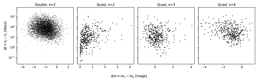
Figure 9: The magnitude difference and the time delays of the mock lensed quasars. The subscripts represent the order of arrival, e.g., $m_{1}$ is the magnitude of the image that arrives first. Most lensed quasars have time lags $\sim 10^{1}-10^{3}$ days. For doubly-imaged quasars, the brighter image usually arrives earlier than the fainter one. For quad lenses, the first-arriving image is the second or third brightest in most cases.

3.3 Statistics of Deflector Galaxies

Figure 10 shows the distribution of the deflector redshift, $z_{d}$, of simulated lensed quasars. The distribution peaks at $z_{d}\sim 0.7$ and drops to a negligible level at $z_{d}\gtrsim 2.5$. This picture is consistent with OM10 and previous modeling of deflector galaxy population (e.g., Hilbert et al., 2008; Wyithe et al., 2011). For comparison, we also include two samples of sources at fixed redshift, $z_{s}=2$ and $z_{s}=5$. Although CosmoDC2 only include galaxies at $z<3$, Figure 10 indicates that only a small fraction of lensed quasars have deflector redshift $z_{d}>3$.

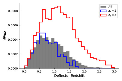
Figure 10: The distribution of deflector redshifts. The $y-$axis denotes the probability for a background source to be lensed by a foreground deflector at a certain redshift. The gray histogram represents all the simulated lensed quasars, which peaks at $\sim 0.7$ and has a median of 0.87. The distribution drops to a negligible level at $z_{d}>2.5$. We also include two samples of background sources at $z_{s}=2$ and $z_{s}=5$ for comparison.

In Figure 11, we present the $i-$band magnitudes of the deflectors and the deflector-to-quasar magnitude difference of the simulated lensed quasars. In nearly all of the LSST-discoverable lensed quasars, the deflector galaxy is brighter than the LSST limit, which suggests that the impact of the foreground galaxy must be considered when selecting lensed quasar candidates. The deflector-to-quasar magnitude difference spreads over a wide range, and the number of quasar-flux-dominated lenses are comparable to that of galaxy-flux-dominated ones. Correspondingly, we expect a large diversity in observed features for lensed quasars. The galaxy-dominated lenses are likely generated by a massive, luminous deflector and have large image separations, and the quasar-dominated ones usually have compact lensing structures. These objects may require very different candidate selection techniques.

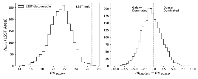
Figure 11: Left: The $i-$band magnitudes of the deflector galaxies of LSST-discoverable lensed quasars. Nearly all of them are beyond the LSST magnitude limit. The impact of deflector galaxy flux must be considered when selecting lensed quasar candidates. Right: the difference between the magnitude of the deflector galaxy and the magnified magnitude of the quasar. The quasar magnitude corresponds to the total flux of all the lensed images of the background quasar. The magnitude difference spreads over a wide range, which suggests a large diversity in observed features for lensed quasars.

4 Discussions

4.1 Choices of QLFs and VDFs

Section 3.1 shows the impact of QLFs and VDFs on the modeling of the lensed quasar population. In this section, we discuss the systematic uncertainties introduced by our choices of QLFs and VDFs.

At $z\lesssim 4$, the QLFs are well-measured down to at least $M_{1450}\sim-22$ (e.g., Richards et al., 2006; Ross et al., 2013; Palanque-Delabrouille et al., 2016), and these measurements are in good agreement with each other. Since most LSST-discoverable lensed quasars have $z_{\text{qso}}<4$, the QLFs adopted by this study provide a good description of the quasar population. Meanwhile, there are still debates about the QLFs at $z\gtrsim 5$. A few studies give a faint-end slope of $\alpha\sim-2$ (e.g., Jiang et al., 2016; Yang et al., 2016; McGreer et al., 2018), while others suggest $\alpha\sim-1.3$ (Niida et al., 2020; Kim et al., 2020). In this work, we use the HSC-based high-redshift QLFs which have $\alpha\sim-1.3$. If the faint-end slope turns out to be steeper, there might be more faint lensed quasars at high redshift.

Unlike the QLFs, the deflector VDFs are not well constrained by spectroscopic surveys beyond the local universe. Many previous studies assumes no evolution of the VDF (e.g., OM10; Wyithe & Loeb, 2002). However, recent analysis of strong lensing systems indicate that the VDF drops towards high redshift (e.g., Geng et al., 2021), which is consistent with photometric measurements (e.g., Bezanson et al., 2011, 2012) and the CosmoDC2 VDFs used in this work. It is thus critical to use redshift-evolving VDF models when modeling the lens population.

In addition, we consider the uncertainties introduced by the scaling relation used to calculate the velocity dispersion (Equation 2). Many studies suggest that the $M_{\text{dyn}}/M_{*}$ ratio evolves with galaxy masses (e.g., Auger et al., 2010; Nigoche-Netro et al., 2016) and redshift (e.g., Beifiori et al., 2014). We thus consider the impact of an evolving $M_{\text{dyn}}/M_{*}$ ratio in the following form:

$$\log\frac{M_{\text{dyn}}}{M_{*}}=a\log(M_{*})+b\log(1+z)+c$$ (5)

This is equivalent to an evolution of $\sigma\propto M_{*}^{a/2}(1+z)^{b/2}$.

We first set $z=0$ to check the mass-dependence. We adopt the relation in Auger et al. (2010), which suggests $\log(M_{*}/M_{\odot})=0.885\log(M_{\text{dyn}}/M_{\odot})+0.905$. The left panel of Figure 12 shows the derived VDF at $z<0.1$, which does not reproduce the observed local VDF. We thus conclude that adding the mass-dependent term does not gives a good description of the galaxy velocity dispersion for the CosmoDC2 catalog.

We then keep the relation $M_{*}/M_{\text{dyn}}=0.557$, and adopt the redshift evolution from Beifiori et al. (2014), which gives $\sigma\propto(1+z)^{0.12}$. The right panel of Figure 12 compares the resulted CosmoDC2 VDF and the observed values in Bezanson et al. (2012). At $z<1$, the redshift evolution makes little difference compare to the original one, and the resulting VDF is still consistent with observation. At $1.2<z<1.5$, the redshift-evolving estimation starts to over-predict the number of galaxies at the massive end, where the observed galaxy sample should be complete. This difference might be more significant at $z>1.5$ where the redshift evolution term gets larger.

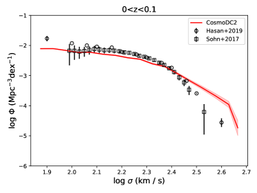
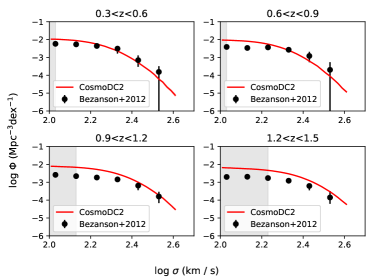
Figure 12: Left: Testing the mass-dependence term in the velocity dispersion. We use the $M_{*}-M_{\text{dyn}}$ relation in Auger et al. (2010) to calculate the velocity dispersion of CosmoDC2 mock galaxies. The resulting local VDF does not match the observations. Right: Testing the redshift-evolution term in the velocity dispersion. We add the redshift-evolution from Beifiori et al. (2014) to the velocity dispersion inferred by Equation 2 for mock galaxies. The redshift evolution is subtle, and the inferred VDF is consistent with observation at $z<1$. However, at $z>1$, the redshift evolution term starts to overpredict the number of galaxies at the massive end.

In addition to the redshift evolution of the velocity dispersion, Beifiori et al. (2014) also reports a redshift evolution of the $M_{\text{dyn}}/M_{*}$ ratio, which follows $M_{\text{dyn}}/M_{*}\propto(1+z)^{-0.30\pm 0.12}$. By including both trends into Equation 2, we get a very subtle evolution of $\sigma\propto(1+z)^{-0.03}$. This result might explain why a non-evolving $M_{\text{dyn}}/M_{*}$ ratio correctly reproduces the observed VDF. In any case, the redshift dependence is subtle. Given the median redshift of deflectors ($z_{d}\sim 0.7$, Figure 10), the evolution will not strongly influence the resulting lensing statistics.

4.2 Mock Catalog Completeness

The CosmoDC2 catalog models dark matter halos down to $10^{9.8}M_{\odot}$. According to the $M_{\text{galaxy}}-M_{\text{halo}}$ relation (e.g., Behroozi et al., 2013), a halo of $\sim 10^{10}M_{\odot}$ usually has $M_{\text{galaxy}}/M_{\text{halo}}\sim 10^{-3}$. The CosmoDC2 catalog should thus be complete down to $M_{*}\sim 10^{7}M_{\odot}$. Our $\sigma-$selected deflector sample has a minimum stellar mass of $M_{*}=10^{7.8}M_{\odot}$, which means that the mock catalog is complete for deflectors with $\sigma>50\text{ km s}^{-1}$ and $z_{\text{d}}<3$.

The main incompleteness comes from the fact that CosmoDC2 catalog only covers $0<z<3$. Figure 10 suggests that the majority of mock lenses have $z_{d}<3$. Wyithe et al. (2011) studies the strong lensing statistics for $z\sim 8$ galaxies, and their results suggest that $>80\%$ lensing systems have $z_{d}<3$. This fraction will be higher for lower source redshifts, and we conclude that our mock catalog is highly complete.

4.3 Finding More Lensed Quasars Beyond the “Discoverable” Ones

In the discussion above, we adopt the definition of a discoverable lensed quasar in OM10, which requires an image separation $\Delta\theta>\frac{2}{3}\times\text{FWHM}$ and a $5\sigma$ detection of the second or third brightest lensed image. The motivation of these criteria is that the lensed quasar images need to be at least marginally resolved and barely visible. Under this definition, about one third of the lensed quasars in the mock catalog are not discoverable in LSST. In this subsection, we discuss possible strategies to find these undiscoverable lenses.

Identifying undiscoverable lensed quasars is important because the discoverable criteria can miss some unique and interesting objects. As an example, Fan et al. (2019) report a compact lens with separation of $0\farcs 2$ at $z=6.51$, J0439+1634, which is the only known multiply-imaged quasar at $z>5$ to date. J0439+1634 has a large magnification of $\mu=51$, making it the brightest quasar at $z>6$ in nearly all wavelengths, and provides so far the best case study of a high-redshift quasar. Although J0439+1634 is bright $(m_{z}=19.49\pm 0.02)$, the small separation makes it undiscoverable in ground-based imaging surveys. Besides, undiscoverable lenses enable many studies that are impossible otherwise. For instance, small-separation lenses can probe the mass distribution of less massive deflector galaxies.

We first consider the image separation criteria. Figure 6 suggests that LSST-like seeing $(\sim 0\farcs 7)$ will be sufficient to resolve the majority of lensed quasars. Lensing systems with smaller separation have less massive and thus fainter deflector galaxies. These objects are likely to have quasar-dominated flux with a marginally extended morphology. Since the deflector galaxy and the lensed quasar images are blended, we expect that neither a PSF nor a regular Sérsic profile can provide a good description of their morphology, according to which we can identify these compact lenses. This method is used in Fan et al. (2019) to identify the $z=6.51$ compact lensed quasar using ground-based imaging, which is later confirmed by HST imaging.

For lensed quasars that do not meet the second criteria, i.e., the fainter lensed image being brighter than the survey limit, some of them can be discovered by identifying the brighter image as a quasar. If there is a bright galaxy next to it, it is a hint that the quasar might be lensed. Figure 11 suggests that the deflector galaxy is detectable in LSST survey in most lensing systems. Follow-up deep imaging and/or spectroscopy can confirm if there is a fainter lensed image. This technique requires decent image de-blending to disentangle the brighter lensed quasar image and the deflector galaxy.

As we show in Figure 11, the observational features of lensed quasars have a large variety. A complete search of them requires a number of distinct candidate selection methods. The mock catalog can serve as training and testing sets for future surveys of lensed quasars with LSST data.

5 Summary and Conclusion

We present a mock catalog of gravitationally lensed quasars at $z_{\text{qso}}<7.5$, which covers quasars with $M_{i}<-20$ and deflector galaxies with $\sigma>50\text{ km s}^{-1}$, using updated QLFs and deflector VDFs. We generate synthetic magnitudes and simulated LSST images for the mock lensed quasars. Using the mock catalog, we explore the expected outputs of lensed quasar surveys, and investigate possible strategies to find more lensed quasars. Our main conclusions are:

1. The number of discoverable lensed quasars in current sky surveys is $\sim 10^{3}$, and LSST will increase this number to $\sim 2.4\times 10^{3}$. Most of the lensed quasars have image separation $\Delta\theta>0\farcs 5$, which will at least get marginally resolved in the LSST survey.

2. There will be $\sim 200$ discoverable quadruply lensed quasars in the LSST survey. The fraction of quad lenses among all discoverable lensed quasars is $\sim 10\%-15\%$ at $m_{i}\lesssim 25$, and decreases with survey depth. The typical time delays between lensed images are $\sim 10^{1}-10^{3}$ days. Follow-up high-cadence observations are necessary to accurately measure the time lags.

3. The mock lensed quasars show a large diversity in their observational features, from deflector-dominated ones which are lensed by bright, massive galaxies with large lensing separations, to quasar-dominated ones which are likely more compact. The variety in observational features requires complex candidate selection techniques.

We estimate that the mock catalog has a high completeness for lensed quasars with Einstein radius $\theta_{E}>0\farcs 07$. This range covers nearly all the lensed quasars that can be identified in the near future, including compact ones that can be discovered by the Euclid Telescope (Laureijs et al., 2011) and the Roman Space Telescope (Spergel et al., 2015). The mock catalog and the simulated images will be powerful tools in future lensed quasar surveys, especially for high-redshift lensed quasars which are not well-explored by previous studies. As an example, we have used the mock catalog to analyze the population of lensed quasars at $z>5$ and design a new survey for these objects (Yue et al. in prep). Besides, although we focus on traditional (point-like) type-I quasars, the code can be easily adapted to study other background source population, including fainter AGNs and normal galaxies.

References

- Agnello et al. (2015) Agnello, A., Kelly, B. C., Treu, T., & Marshall, P. J. 2015, MNRAS, 448, 1446, doi: 10.1093/mnras/stv037
- Agnello et al. (2018) Agnello, A., Schechter, P. L., Morgan, N. D., et al. 2018, MNRAS, 475, 2086, doi: 10.1093/mnras/stx3226
- Aihara et al. (2018a) Aihara, H., Armstrong, R., Bickerton, S., et al. 2018a, PASJ, 70, S8, doi: 10.1093/pasj/psx081
- Aihara et al. (2018b) Aihara, H., Arimoto, N., Armstrong, R., et al. 2018b, PASJ, 70, S4, doi: 10.1093/pasj/psx066
- Akiyama et al. (2018) Akiyama, M., He, W., Ikeda, H., et al. 2018, PASJ, 70, S34, doi: 10.1093/pasj/psx091
- Astropy Collaboration et al. (2013) Astropy Collaboration, Robitaille, T. P., Tollerud, E. J., et al. 2013, A&A, 558, A33, doi: 10.1051/0004-6361/201322068
- Astropy Collaboration et al. (2018) Astropy Collaboration, Price-Whelan, A. M., Sipőcz, B. M., et al. 2018, AJ, 156, 123, doi: 10.3847/1538-3881/aabc4f
- Auger et al. (2010) Auger, M. W., Treu, T., Bolton, A. S., et al. 2010, ApJ, 724, 511, doi: 10.1088/0004-637X/724/1/511
- Behroozi et al. (2019) Behroozi, P., Wechsler, R. H., Hearin, A. P., & Conroy, C. 2019, MNRAS, 488, 3143, doi: 10.1093/mnras/stz1182
- Behroozi et al. (2013) Behroozi, P. S., Wechsler, R. H., & Conroy, C. 2013, ApJ, 770, 57, doi: 10.1088/0004-637X/770/1/57
- Beifiori et al. (2014) Beifiori, A., Thomas, D., Maraston, C., et al. 2014, ApJ, 789, 92, doi: 10.1088/0004-637X/789/2/92
- Bertin et al. (2002) Bertin, G., Ciotti, L., & Del Principe, M. 2002, A&A, 386, 149, doi: 10.1051/0004-6361:20020248
- Bezanson et al. (2012) Bezanson, R., van Dokkum, P., & Franx, M. 2012, ApJ, 760, 62, doi: 10.1088/0004-637X/760/1/62
- Bezanson et al. (2011) Bezanson, R., van Dokkum, P. G., Franx, M., et al. 2011, ApJ, 737, L31, doi: 10.1088/2041-8205/737/2/L31
- Brown et al. (2014) Brown, M. J. I., Moustakas, J., Smith, J. D. T., et al. 2014, ApJS, 212, 18, doi: 10.1088/0067-0049/212/2/18
- Cappellari et al. (2006) Cappellari, M., Bacon, R., Bureau, M., et al. 2006, MNRAS, 366, 1126, doi: 10.1111/j.1365-2966.2005.09981.x
- Cashman et al. (2021) Cashman, F. H., Kulkarni, V. P., & Lopez, S. 2021, AJ, 161, 90, doi: 10.3847/1538-3881/abd2b0
- Chambers et al. (2016) Chambers, K. C., Magnier, E. A., Metcalfe, N., et al. 2016, arXiv e-prints, arXiv:1612.05560. https://arxiv.org/abs/1612.05560
- Chan et al. (2020) Chan, J. H. H., Suyu, S. H., Sonnenfeld, A., et al. 2020, A&A, 636, A87, doi: 10.1051/0004-6361/201937030
- Choi et al. (2007) Choi, Y.-Y., Park, C., & Vogeley, M. S. 2007, ApJ, 658, 884, doi: 10.1086/511060
- Collett (2015) Collett, T. E. 2015, ApJ, 811, 20, doi: 10.1088/0004-637X/811/1/20
- Cornachione & Morgan (2020) Cornachione, M. A., & Morgan, C. W. 2020, ApJ, 895, 93, doi: 10.3847/1538-4357/ab8aed
- DES Collaboration et al. (2021) DES Collaboration, Abbott, T. M. C., Adamow, M., et al. 2021, arXiv e-prints, arXiv:2101.05765. https://arxiv.org/abs/2101.05765
- Dey et al. (2019) Dey, A., Schlegel, D. J., Lang, D., et al. 2019, AJ, 157, 168, doi: 10.3847/1538-3881/ab089d
- Fan et al. (2019) Fan, X., Wang, F., Yang, J., et al. 2019, ApJ, 870, L11, doi: 10.3847/2041-8213/aaeffe
- Geng et al. (2021) Geng, S., Cao, S., Liu, Y., et al. 2021, MNRAS, 503, 1319, doi: 10.1093/mnras/stab519
- Gilman et al. (2020) Gilman, D., Birrer, S., Nierenberg, A., et al. 2020, MNRAS, 491, 6077, doi: 10.1093/mnras/stz3480
- Harris et al. (2020) Harris, C. R., Millman, K. J., van der Walt, S. J., et al. 2020, Nature, 585, 357, doi: 10.1038/s41586-020-2649-2
- Hasan & Crocker (2019) Hasan, F., & Crocker, A. 2019, arXiv e-prints, arXiv:1904.00486. https://arxiv.org/abs/1904.00486
- Heitmann et al. (2019) Heitmann, K., Finkel, H., Pope, A., et al. 2019, ApJS, 245, 16, doi: 10.3847/1538-4365/ab4da1
- Hilbert et al. (2009) Hilbert, S., Hartlap, J., White, S. D. M., & Schneider, P. 2009, A&A, 499, 31, doi: 10.1051/0004-6361/200811054
- Hilbert et al. (2008) Hilbert, S., White, S. D. M., Hartlap, J., & Schneider, P. 2008, MNRAS, 386, 1845, doi: 10.1111/j.1365-2966.2008.13190.x
- Inada et al. (2012) Inada, N., Oguri, M., Shin, M.-S., et al. 2012, AJ, 143, 119, doi: 10.1088/0004-6256/143/5/119
- Ivezić et al. (2019) Ivezić, Ž., Kahn, S. M., Tyson, J. A., et al. 2019, ApJ, 873, 111, doi: 10.3847/1538-4357/ab042c
- Jaelani et al. (2021) Jaelani, A. T., Rusu, C. E., Kayo, I., et al. 2021, MNRAS, 502, 1487, doi: 10.1093/mnras/stab145
- Jiang et al. (2016) Jiang, L., McGreer, I. D., Fan, X., et al. 2016, ApJ, 833, 222, doi: 10.3847/1538-4357/833/2/222
- Kim et al. (2020) Kim, Y., Im, M., Jeon, Y., et al. 2020, ApJ, 904, 111, doi: 10.3847/1538-4357/abc0ea
- Kochanek et al. (2006) Kochanek, C. S., Mochejska, B., Morgan, N. D., & Stanek, K. Z. 2006, ApJ, 637, L73, doi: 10.1086/500559
- Kormann et al. (1994) Kormann, R., Schneider, P., & Bartelmann, M. 1994, A&A, 284, 285
- Korytov et al. (2019) Korytov, D., Hearin, A., Kovacs, E., et al. 2019, ApJS, 245, 26, doi: 10.3847/1538-4365/ab510c
- Laureijs et al. (2011) Laureijs, R., Amiaux, J., Arduini, S., et al. 2011, arXiv e-prints, arXiv:1110.3193. https://arxiv.org/abs/1110.3193
- Lawrence et al. (2007) Lawrence, A., Warren, S. J., Almaini, O., et al. 2007, MNRAS, 379, 1599, doi: 10.1111/j.1365-2966.2007.12040.x
- Lemon et al. (2020) Lemon, C., Auger, M. W., McMahon, R., et al. 2020, MNRAS, 494, 3491, doi: 10.1093/mnras/staa652
- Lemon et al. (2019) Lemon, C. A., Auger, M. W., & McMahon, R. G. 2019, MNRAS, 483, 4242, doi: 10.1093/mnras/sty3366
- Lemon et al. (2018) Lemon, C. A., Auger, M. W., McMahon, R. G., & Ostrovski, F. 2018, MNRAS, 479, 5060, doi: 10.1093/mnras/sty911
- LSST Science Collaboration et al. (2009) LSST Science Collaboration, Abell, P. A., Allison, J., et al. 2009, arXiv e-prints, arXiv:0912.0201. https://arxiv.org/abs/0912.0201
- Luhtaru et al. (2021) Luhtaru, R., Schechter, P. L., & de Soto, K. M. 2021, ApJ, 915, 4, doi: 10.3847/1538-4357/abfda1
- Mao et al. (2018) Mao, Y.-Y., Kovacs, E., Heitmann, K., et al. 2018, ApJS, 234, 36, doi: 10.3847/1538-4365/aaa6c3
- Matsuoka et al. (2018) Matsuoka, Y., Strauss, M. A., Kashikawa, N., et al. 2018, ApJ, 869, 150, doi: 10.3847/1538-4357/aaee7a
- McGreer et al. (2018) McGreer, I. D., Fan, X., Jiang, L., & Cai, Z. 2018, AJ, 155, 131, doi: 10.3847/1538-3881/aaaab4
- McGreer et al. (2010) McGreer, I. D., Hall, P. B., Fan, X., et al. 2010, AJ, 140, 370, doi: 10.1088/0004-6256/140/2/370
- McGreer et al. (2013) McGreer, I. D., Jiang, L., Fan, X., et al. 2013, ApJ, 768, 105, doi: 10.1088/0004-637X/768/2/105
- More et al. (2016) More, A., Oguri, M., Kayo, I., et al. 2016, MNRAS, 456, 1595, doi: 10.1093/mnras/stv2813
- Nigoche-Netro et al. (2016) Nigoche-Netro, A., Ramos-Larios, G., Lagos, P., et al. 2016, MNRAS, 462, 951, doi: 10.1093/mnras/stw1661
- Niida et al. (2020) Niida, M., Nagao, T., Ikeda, H., et al. 2020, ApJ, 904, 89, doi: 10.3847/1538-4357/abbe11
- Oguri (2006) Oguri, M. 2006, MNRAS, 367, 1241, doi: 10.1111/j.1365-2966.2006.10043.x
- Oguri (2010) —. 2010, PASJ, 62, 1017, doi: 10.1093/pasj/62.4.1017
- Oguri & Marshall (2010) Oguri, M., & Marshall, P. J. 2010, MNRAS, 405, 2579, doi: 10.1111/j.1365-2966.2010.16639.x
- Palanque-Delabrouille et al. (2016) Palanque-Delabrouille, N., Magneville, C., Yèche, C., et al. 2016, A&A, 587, A41, doi: 10.1051/0004-6361/201527392
- Paraficz et al. (2018) Paraficz, D., Rybak, M., McKean, J. P., et al. 2018, A&A, 613, A34, doi: 10.1051/0004-6361/201731250
- Peng et al. (2002) Peng, C. Y., Ho, L. C., Impey, C. D., & Rix, H.-W. 2002, AJ, 124, 266, doi: 10.1086/340952
- Richards et al. (2006) Richards, G. T., Strauss, M. A., Fan, X., et al. 2006, AJ, 131, 2766, doi: 10.1086/503559
- Ross et al. (2013) Ross, N. P., McGreer, I. D., White, M., et al. 2013, ApJ, 773, 14, doi: 10.1088/0004-637X/773/1/14
- Sohn et al. (2017) Sohn, J., Zahid, H. J., & Geller, M. J. 2017, ApJ, 845, 73, doi: 10.3847/1538-4357/aa7de3
- Spergel et al. (2015) Spergel, D., Gehrels, N., Baltay, C., et al. 2015, arXiv e-prints, arXiv:1503.03757. https://arxiv.org/abs/1503.03757
- Spiniello et al. (2018) Spiniello, C., Agnello, A., Napolitano, N. R., et al. 2018, MNRAS, 480, 1163, doi: 10.1093/mnras/sty1923
- Suyu et al. (2017) Suyu, S. H., Bonvin, V., Courbin, F., et al. 2017, MNRAS, 468, 2590, doi: 10.1093/mnras/stx483
- Treu et al. (2018) Treu, T., Agnello, A., Baumer, M. A., et al. 2018, MNRAS, 481, 1041, doi: 10.1093/mnras/sty2329
- van der Walt et al. (2011) van der Walt, S., Colbert, S. C., & Varoquaux, G. 2011, Computing in Science and Engineering, 13, 22, doi: 10.1109/MCSE.2011.37
- Wang et al. (2019) Wang, F., Yang, J., Fan, X., et al. 2019, ApJ, 884, 30, doi: 10.3847/1538-4357/ab2be5
- Wright et al. (2010) Wright, E. L., Eisenhardt, P. R. M., Mainzer, A. K., et al. 2010, AJ, 140, 1868, doi: 10.1088/0004-6256/140/6/1868
- Wyithe & Loeb (2002) Wyithe, J. S. B., & Loeb, A. 2002, ApJ, 577, 57, doi: 10.1086/342181
- Wyithe et al. (2011) Wyithe, J. S. B., Yan, H., Windhorst, R. A., & Mao, S. 2011, Nature, 469, 181, doi: 10.1038/nature09619
- Yang et al. (2016) Yang, J., Wang, F., Wu, X.-B., et al. 2016, ApJ, 829, 33, doi: 10.3847/0004-637X/829/1/33
- Yang et al. (2019) Yang, J., Venemans, B., Wang, F., et al. 2019, ApJ, 880, 153, doi: 10.3847/1538-4357/ab2a02
- York et al. (2000) York, D. G., Adelman, J., Anderson, John E., J., et al. 2000, AJ, 120, 1579, doi: 10.1086/301513
- Yue et al. (2021a) Yue, M., Fan, X., Yang, J., & Wang, F. 2021a, arXiv e-prints, arXiv:2112.02821. https://arxiv.org/abs/2112.02821
- Yue et al. (2021b) Yue, M., Yang, J., Fan, X., et al. 2021b, ApJ, 917, 99, doi: 10.3847/1538-4357/ac0af4