NCTS-HEPAP/2201

Taking Neutrino Pictures via Electrons

Guey-Lin Lin${}^{\,a,}$ , Thi Thuy Linh Nguyen${}^{\,a,}$ , Martin Spinrath${}^{\,b,c}$ , Thi Dieu Hien Van${}^{\,a,}$

and Tse-Chun Wang${}^{\,d,}$

^a Institute of Physics, National Yang Ming Chiao Tung University, Hsinchu 300, Taiwan

^b Department of Physics, National Tsing Hua University, Hsinchu, 30013, Taiwan

^c Center for Theory and Computation, National Tsing Hua University, Hsinchu 300, Taiwan

^d Physics Division, National Center for Theoretical Sciences, Taipei 10617, Taiwan

In this paper we discuss the prospects to take a picture of an extended neutrino source, i.e., resolving its angular neutrino luminosity distribution. This is challenging since neutrino directions cannot be directly measured but only estimated from the directions of charged particles they interact with in the detector material. This leads to an intrinsic blurring effect. We first discuss the problem in general terms and then apply our insights to solar neutrinos scattering elastically with electrons. Despite the aforementioned blurring we show how with high statistics and precision the original neutrino distributions could be reconstructed.

1 Introduction

Astronomy is one of the oldest scientific endeavours of mankind which received a huge boost in the last century with the invention of telescopes sensitive to photons over a huge range of energies far above and below the optical spectrum which is also still improving and expanding. This progress is based to a large extent on an improved physical understanding of the properties and the nature of light or photons and its interactions with matter. This advancement allowed to resolve the true nature of planets, moons and other objects in the solar system which seem point-like without telescopes.

But photons are not the only messengers of astronomical sources routinely being studied. In this paper we will focus on neutrinos which similarly have gained importance for astrophysics due to the improved and still constantly improving understanding of their nature and origin driven by particle physics. Latest since the observation of solar neutrinos by the Homestake experiment - see, e.g., [1] for a review on the experiment and [2] for a recent review of solar neutrinos - and the detection of neutrinos from supernova SN1987A [3, 4, 5] they have established themselves as an important tool in astrophysics. Also the studied energy range of neutrinos has expanded significantly culminating in neutrino telescopes such as IceCube [6] and KM3NET [7]. The simultaneous observation of photons and neutrinos from the same astrophysical sources is the template for modern multimessenger astroparticle physics which recently gained an additional boost by the observation of gravitational waves.

Neutrinos are interesting as astrophysical messengers since they travel almost freely not taking part in electromagnetic and strong interactions, for a recent review, see, for instance, [8]. Indeed, very often neutrinos are produced inside of stars and then escape with small distortions compared to other messengers. It takes extreme events like supernovae to affect neutrinos substantially on their path and even then neutrinos are the first messengers escaping and giving valuable information on the earliest stages of a supernova [9, 10, 11]. For that reason they are being used, for instance, in an alarm system to point other telescopes to interesting astrophysical events [12, 13, 14, 15, 16, 17].

The drawback is that neutrinos are also hard to detect for the very same reasons. And in all experiments their detection happens indirectly via elastic or inelastic processes sometimes eradicating substantial information about the original neutrino energy, direction and flavour [12, 14, 15, 18, 17]. In this paper we will focus on elastic scattering processes which still introduce quite some uncertainty in the reconstruction of the incident neutrino energy and direction in an individual event and we compare our results to the results from [18]. Since there are new experiments coming up or proposed with improved detection capabilities and analysis techniques (e.g., the Hyper-Kamiokande (HyperK) experiment [19], the Jiangmen Underground Neutrino Observatory (JUNO) [20, 21], the SNO$+$ experiment [22], IceCube-GEN2 [23], the Precision IceCube Next Generation Upgrade (PINGU) [24], KM3NeT [7], etc), we think it is the right time to go beyond point-like neutrino sources in the sky and study if we can resolve their structures.

In this work we establish a framework which would allow, in principle, to reconstruct the picture of an extended source in “neutrino light” and apply this framework explicitly to solar neutrinos which are understood rather well from theory and experiment. As a guiding question we will ask if it is possible to distinguish a point source and a ring-shaped source the size of the sun for neutrinos with an energy spectrum and flavour composition as solar neutrinos. We will focus here on the electron picture and not explicitly reconstruct the neutrino picture since, in particular, the inclusion of experimental uncertainties make a reconstruction of the solar neutrino pictures with a sufficient resolution quite difficult at this point. We find that the distinction between a point and a ring source just from the electron picture is rather hard but theoretically possible.

Nevertheless, if we would be able to reconstruct the neutrino picture successfully with high precision – and we consider our work presented here as a step in this direction – it would offer a way to distinguish different solar models and help to reconstruct a full three-dimensional model of the sun including things like temperature and pressure profiles. They are connected to the radial neutrino flux profiles of the sun which we will translate into two-dimensional angular luminosity distributions of neutrinos, the neutrino pictures. Different from Ref. [18], for a better understanding of the physics inside the sun (or other sources), we analyse both angular and energy distributions of solar neutrino events, in terms of the double differential event rate later in this work. The double differential event rate ideally helps us as well to measure the spatial separation of different neutrino sources. From our results it will also be clear for which kind of sources it could lead to a less blurry picture than for solar neutrinos.

This paper is arranged as follows: We will first derive in Sec. 2 the theoretical framework and show how the observed energy and angular distributions of scattered electrons are related to the energy and angular distribution of the incoming neutrino flux. Interestingly, they are related by an invertible integral transformation which involves the differential cross section as well. In Sec. 3 we apply this framework to some simple toy examples and also make a first step towards answering, how large the neutrino picture of the sun is. In Sec. 4 we discuss the fully realistic case for ⁸B, hep and pep solar neutrinos and their pictures. Then we illustrate how those pictures could be affected by experimental errors in Sec. 5 before we summarise and conclude in Sec. 6. We also provide extensive appendices with additional details on the derivation of the formulas in the main text.

2 Theoretical Framework

To take a neutrino picture of any extended neutrino source one has to consider the scattering of neutrinos in the detector material. Here we will focus on solar neutrinos with an energy around 10 MeV and adopt neutrino electron elastic scattering $\nu+e^{-}\rightarrow\nu+e^{-}$. All flavors of neutrinos (and for other sources anti-neutrinos) can be detected by this interaction, though the cross sections depend on flavour and chirality. We will show here how to reconstruct the angular and energy distribution of neutrinos by measuring the direction and energy of the scattered electrons. In this section, we first build the theoretical framework for this methodology and then study applications in the rest of the paper.

A very similar exercise was done for directional Dark Matter (DM) detection and we will follow this approach as presented in [25] closely here. There is one major difference between DM and our case that is that the incoming neutrinos here are highly relativistic and hence practically massless while the incoming DM particles there are assumed to be non-relativistic.

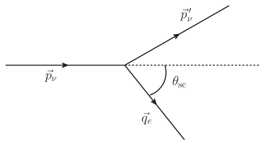
Figure 1: Sketch to clarify the kinematics used in Sec. 2.

We want to assume that the electrons in our target are at rest and free (we neglect binding energies here). The relativistic energy momentum conservation then reads, cf. Fig. 1,

$$\sqrt{m_{\nu}^{2}+p_{\nu}^{2}}+m_{e} =\sqrt{m_{\nu}^{2}+{p^{\prime}}_{\nu}^{2}}+\sqrt{m_{e}^{2}+q_{e}^{2}}\;,$$ (2.1)

$$p^{\prime}_{\nu}\cos\theta_{\text{sc}} =p_{\nu}-q_{e}\cos\theta_{\text{sc}}\;,$$ (2.2)

$$p^{\prime}_{\nu}\sin\theta_{\text{sc}} =q_{e}\sin\theta_{\text{sc}}\;,$$ (2.3)

where $m_{\nu}$, $p_{\nu}$ and $p^{\prime}_{\nu}$ are neutrino mass and modulus of three-momentum before and after scattering. The mass of the electron is $m_{e}$ and the modulus of its three-momentum after scattering is $q_{e}$. The scattering angle with respect to the incoming neutrino direction is defined as $\theta_{\text{sc}}$.

We can sum the squares of the last two equations to get

$${p^{\prime}}_{\nu}^{2}=(p_{\nu}-q_{e}\cos\theta_{\text{sc}})^{2}+(q_{e}\sin\theta_{\text{sc}})^{2}=p_{\nu}^{2}-2p_{\nu}q_{e}\cos\theta_{\text{sc}}+q_{e}^{2}$$ (2.4)

and use this equation to eliminate ${p^{\prime}}_{\nu}^{2}$ from the first equation. Using the relativistic approximation $m_{\nu}\ll p_{\nu}\approx E_{\nu}$ we then find

$$\cos\theta_{\text{sc}} =\frac{(E_{e}-m_{e})(E_{\nu}+m_{e})}{E_{\nu}\,\sqrt{E_{e}^{2}-m_{e}^{2}}}=\hat{p}_{\nu}\cdot\hat{q}_{e}\;,$$ (2.5)

where we have noted that the cosine of the scattering angle between the incoming neutrino direction and the outgoing electron direction can be written in a coordinate independent way as the scalar product of the normalised momentum vectors of the incoming neutrino and the outgoing electron. The outgoing electron energy is restricted to the range

$$m_{e}\leq E_{e}\leq\frac{2E_{\nu}^{2}+2E_{\nu}\,m_{e}+m_{e}^{2}}{2E_{\nu}+m_{e}}\equiv E_{e}^{\text{max}}$$ (2.6)

corresponding to $0\leq\cos\theta_{\text{sc}}\leq 1\;$. We want to remind here that $E_{e}$ is the total electron energy after scattering including the electron mass, and the electron kinetic energy $T_{e}=E_{e}-m_{e}$ as labeled.

Our aim here is to derive an expression for the double differential event rate, in events per unit time per unit detector mass, differentiated with respect to the electron energy $E_{e}$ and electron recoil direction $\hat{q}_{e}$

$$\frac{\operatorname{\text{d}}R}{\operatorname{\text{d}}E_{e}\operatorname{\text{d}}\Omega_{e}}\;,$$ (2.7)

where $\operatorname{\text{d}}\Omega_{e}$ denotes the infinitesimal solid angle around the direction $\hat{q}_{e}$.

The double differential rate follows from the double differential cross section

$$\frac{\operatorname{\text{d}}\sigma}{\operatorname{\text{d}}E_{e}\operatorname{\text{d}}\Omega_{e}}\;.$$ (2.8)

In the scattering processes we consider here the electron energy $E_{e}$ and scattering direction are not independent from each other. But we can impose their relation explicitly with a $\delta$-function using eq. (2.5)

$$\frac{\operatorname{\text{d}}\sigma}{\operatorname{\text{d}}E_{e}\operatorname{\text{d}}\Omega_{e}}=\frac{\operatorname{\text{d}}\sigma}{\operatorname{\text{d}}E_{e}}\frac{1}{2\pi}\delta\left(\hat{p}_{\nu}\cdot\hat{q}_{e}-\frac{(E_{e}-m_{e})(E_{\nu}+m_{e})}{E_{\nu}\,\sqrt{E_{e}^{2}-m_{e}^{2}}}\right)\;.$$ (2.9)

This is crucial and was already done in [25] which nevertheless looks somewhat different there due to the different kinematics.

Now to go from the double differential cross section to the double differential event rate we have to multiply the first with the number of electrons in the detector $N_{e}$, divide by its mass $M_{D}$ and multiply with the flux of incoming neutrinos. Again, since we talk about incoming relativistic particles we will deviate from the presentation in [25] somewhat. The number flux element in our case is given by

$$\frac{\operatorname{\text{d}}F(E_{\nu},\Omega_{\nu})}{\operatorname{\text{d}}E_{\nu}\operatorname{\text{d}}\Omega_{\nu}}\operatorname{\text{d}}E_{\nu}\operatorname{\text{d}}\Omega_{\nu}\;.$$ (2.10)

For solar neutrinos the distributions of energy and direction of incoming neutrinos are to a good approximation independent from each other, and we can write

$$\frac{\operatorname{\text{d}}F(E_{\nu},\Omega_{\nu})}{\operatorname{\text{d}}E_{\nu}\operatorname{\text{d}}\Omega_{\nu}}\operatorname{\text{d}}E_{\nu}\operatorname{\text{d}}\Omega_{\nu}=f_{0}\frac{\operatorname{\text{d}}\epsilon(E_{\nu})}{\operatorname{\text{d}}E_{\nu}}\frac{\operatorname{\text{d}}\lambda(\Omega_{\nu})}{\operatorname{\text{d}}\Omega_{\nu}}\operatorname{\text{d}}E_{\nu}\operatorname{\text{d}}\Omega_{\nu}\;,$$ (2.11)

where the energy and angular distributions itself are normalised, i.e.,

$$\int\operatorname{\text{d}}E_{\nu}\frac{\operatorname{\text{d}}\epsilon(E_{\nu})}{\operatorname{\text{d}}E_{\nu}}=1\quad\text{ and }\quad\int\operatorname{\text{d}}\Omega_{\nu}\frac{\operatorname{\text{d}}\lambda(\Omega_{\nu})}{\operatorname{\text{d}}\Omega_{\nu}}=1\;.$$ (2.12)

Then

$$\frac{\operatorname{\text{d}}R}{\operatorname{\text{d}}E_{e}\operatorname{\text{d}}\Omega_{e}} =\frac{N_{e}}{M_{D}}\int\operatorname{\text{d}}E_{\nu}\operatorname{\text{d}}\Omega_{\nu}\frac{\operatorname{\text{d}}\sigma(E_{e},E_{\nu})}{\operatorname{\text{d}}E_{e}\operatorname{\text{d}}\Omega_{e}}\frac{\operatorname{\text{d}}F(E_{\nu},\Omega_{\nu})}{\operatorname{\text{d}}E_{\nu}\operatorname{\text{d}}\Omega_{\nu}}$$

$$=\frac{N_{e}\,f_{0}}{2\pi\,M_{D}}\int\operatorname{\text{d}}E_{\nu}\,\frac{\operatorname{\text{d}}\epsilon(E_{\nu})}{\operatorname{\text{d}}E_{\nu}}\frac{\operatorname{\text{d}}\sigma(E_{e},E_{\nu})}{\operatorname{\text{d}}E_{e}}\,$$

$$\quad\times\int\operatorname{\text{d}}\Omega_{\nu}\frac{\operatorname{\text{d}}\lambda(\Omega_{\nu})}{\operatorname{\text{d}}\Omega_{\nu}}\delta\left(\hat{p}_{\nu}\cdot\hat{q}_{e}-\frac{(E_{e}-m_{e})(E_{\nu}+m_{e})}{E_{\nu}\,\sqrt{E_{e}^{2}-m_{e}^{2}}}\right)\;.$$ (2.13)

This equation is the key formula which we will use throughout the rest of the paper.

What is interesting about this is that by measuring the double differential scattered electron rate, it is possible to infer the original neutrino distributions. For DM the author of [25] has shown that the double differential event rate is proportional to the Radon transform of the DM velocity distribution. In our case this is again not quite that easy but we can find an analogous result.

We start from rewriting our key formula eq. (2.13) and after using that $E_{\nu}=|\vec{p}_{\nu}|$ and $E_{\nu}^{2}\operatorname{\text{d}}E_{\nu}\operatorname{\text{d}}\Omega_{\nu}=\operatorname{\text{d}}^{3}\vec{p}_{\nu}$,

$$\frac{\operatorname{\text{d}}R}{\operatorname{\text{d}}E_{e}\operatorname{\text{d}}\Omega_{e}} =\frac{N_{e}\,f_{0}}{2\pi\,M_{D}}\int\operatorname{\text{d}}^{3}\vec{p}_{\nu}\frac{\operatorname{\text{d}}\epsilon}{\operatorname{\text{d}}|\vec{p}_{\nu}|}\frac{\operatorname{\text{d}}\lambda(\Omega_{\nu})}{\operatorname{\text{d}}\Omega_{\nu}}\frac{1}{|\vec{p}_{\nu}|}\frac{\operatorname{\text{d}}\sigma}{\operatorname{\text{d}}E_{e}}(E_{e},|\vec{p}_{\nu}|)\,$$

$$\quad\times\delta\left(\vec{p}_{\nu}\cdot\hat{q}_{e}-\frac{(E_{e}-m_{e})(|\vec{p}_{\nu}|+m_{e})}{\sqrt{E_{e}^{2}-m_{e}^{2}}}\right)\;.$$ (2.14)

Now we can define the generalised distribution analogous to the DM velocity distribution

$$g(E_{e},\vec{p}_{\nu})\equiv f_{0}\frac{\operatorname{\text{d}}\epsilon}{\operatorname{\text{d}}|\vec{p}_{\nu}|}\frac{\operatorname{\text{d}}\lambda(\Omega_{\nu})}{\operatorname{\text{d}}\Omega_{\nu}}\frac{1}{|\vec{p}_{\nu}|}\frac{\operatorname{\text{d}}\sigma}{\operatorname{\text{d}}E_{e}}(E_{e},|\vec{p}_{\nu}|)$$ (2.15)

and the vector

$$\vec{w}=\frac{(E_{e}-m_{e})(E_{\nu}+m_{e})}{\sqrt{E_{e}^{2}-m_{e}^{2}}}\hat{q}_{e}\;,$$ (2.16)

which is parallel to the electron recoil direction $\hat{q}_{e}$ but has a different length, $w$. We arrive at the double differential rate

$$\frac{\operatorname{\text{d}}R}{\operatorname{\text{d}}E_{e}\operatorname{\text{d}}\Omega_{e}} =\frac{N_{e}}{2\pi\,M_{D}}\int\operatorname{\text{d}}^{3}\vec{p}_{\nu}\,g(E_{e},\vec{p}_{\nu})\,\delta\left(\vec{p}_{\nu}\cdot\hat{w}-w\right)=\frac{N_{e}}{2\pi\,M_{D}}\widehat{g}(w,\hat{w})\;.$$ (2.17)

At this point the Radon transform of the distribution function

$$\widehat{g}(w,\hat{w})=\int\operatorname{\text{d}}^{3}\vec{p}_{\nu}\,g(E_{e},\vec{p}_{\nu})\,\delta\left(\vec{p}_{\nu}\cdot\hat{w}-w\right)$$ (2.18)

appears. In the case of DM the distribution function $g$ was actually just the DM velocity distribution which does not depend on the electron energy. In our case, this is more complicated due to the relativistic nature of the incoming neutrinos and since we also do not assume the cross section to be approximately constant over the considered momentum range as can be done for many DM models.

In [25] the author also mentions some ways to invert the Radon transform. This is indeed a common, well studied problem since this transform plays an important role, for instance, in medical imaging. Using that inversion techniques one could hence derive the function $g(E_{e},\vec{p}_{\nu})$ after measuring the double differential event rate. To get the angular distribution of the neutrinos one would then still need to have knowledge of the neutrino energy spectrum and the differential neutrino electron cross section. Monochromatic sources where all neutrinos have the same energy would hence be particularly well suited subjects of study.

The cross section is well known and we use here the result from [26] which we have collected for the convenience of the reader in App. A rewritten in terms of $E_{e}$ as we will need it.

3 Some simplified examples

Before we consider the fully realistic example of solar neutrinos we want to discuss two simple toy examples first. The ultimate goal of this exercise would be to resolve a non-trivial angular distribution of a given neutrino source. To do this we want to study two extreme examples, a point and a ring source (we study radial symmetric sources throughout this paper). The question is then, could we actually distinguish a point from a ring source?

3.1 Monochromatic Point vs. Ring Source

Let us first discuss the point source. In the examples we will always choose the lab frame such that the center of the radial symmetric source is in positive $z$-direction (at $\cos\theta_{e,\nu}=1$). We also assume for now that the neutrino source is monochromatic, that means all neutrinos have the same energy, $E_{\nu}=E_{0}$.

For the point source we then assume the following angular and energy distributions

$$\frac{\operatorname{\text{d}}\lambda_{p}(\Omega_{\nu})}{\operatorname{\text{d}}\Omega_{\nu}}=\frac{1}{2\pi}\delta(\cos\theta_{\nu}-1)\text{ and }\frac{\operatorname{\text{d}}\epsilon_{p}(E_{\nu})}{\operatorname{\text{d}}E_{\nu}}=\delta(E_{\nu}-E_{0})\;.$$ (3.1)

We can then derive the double differential rate as (we provide more details of the derivations of the relevant formulas in this section in App. B)

$$\frac{\operatorname{\text{d}}R_{p}}{\operatorname{\text{d}}E_{e}\operatorname{\text{d}}\Omega_{e}} =\frac{N_{e}\,f_{0}}{2\pi\,M_{D}}\frac{\operatorname{\text{d}}\sigma}{\operatorname{\text{d}}E_{e}}(E_{e},E_{\nu}=E_{0})\,\delta\left(\cos\theta_{e}-\frac{(E_{e}-m_{e})(E_{0}+m_{e})}{E_{0}\sqrt{E_{e}^{2}-m_{e}^{2}}}\right)$$

$$\equiv\gamma_{p}\,\delta\left(\cos\theta_{e}-\frac{(E_{e}-m_{e})(E_{0}+m_{e})}{E_{0}\sqrt{E_{e}^{2}-m_{e}^{2}}}\right)\;,$$ (3.2)

where we have defined $\gamma_{p}$ which we will use later. At this point one could choose to integrate over the electron energy or the electron angular distribution depending on what one is interested in. To show an explicit example, we integrate over the electron energy from a threshold value $E_{e}^{\text{thr}}$ to infinity to get the angular distribution

$$\frac{\operatorname{\text{d}}R_{p}}{\operatorname{\text{d}}\Omega_{e}} =\int_{E_{e}^{\text{thr}}}^{\infty}\operatorname{\text{d}}E_{e}\frac{\operatorname{\text{d}}R_{p}}{\operatorname{\text{d}}E_{e}\operatorname{\text{d}}\Omega_{e}}$$

$$=\frac{N_{e}\,f_{0}}{2\pi\,M_{D}}\frac{\operatorname{\text{d}}\sigma}{\operatorname{\text{d}}E_{e}}\left(E_{\nu}=E_{0},E_{e}=E_{e}^{(p)}\right)\,\theta(E_{e}^{(p)}-E_{e}^{\text{thr}})\frac{E_{0}(E_{e}^{(p)}+m_{e})\sqrt{(E_{e}^{(p)})^{2}-m_{e}^{2}}}{m_{e}(E_{0}+m_{e})}\;,$$ (3.3)

where

$$E_{e}^{(p)}=m_{e}\frac{E_{0}^{2}(\cos^{2}\theta_{e}+1)+2\,m_{e}\,E_{0}+m_{e}^{2}}{E_{0}^{2}\sin^{2}\theta_{e}+2\,m_{e}\,E_{0}+m_{e}^{2}}\;.$$ (3.4)

To go from this solid angle distribution to the simple angular distribution $\operatorname{\text{d}}R_{p}/\operatorname{\text{d}}\cos\theta_{e}$ one would simple have to multiply by $2\pi$ due to the radial symmetry.

Let us now consider a monochromatic ring source, i.e.,

$$\frac{\operatorname{\text{d}}\lambda_{r}(\Omega_{\nu})}{\operatorname{\text{d}}\Omega_{\nu}}=\frac{1}{2\pi}\delta\left(\cos\theta_{\nu}-c_{r}\right)\text{ and }\frac{\operatorname{\text{d}}\epsilon_{r}(E_{\nu})}{\operatorname{\text{d}}E_{\nu}}=\delta(E_{\nu}-E_{0})\;,$$ (3.5)

where we do not yet specify the opening angle of the ring but assume it is small, $1\gg 1-c_{r}^{2}>0$. We then find for the double differential event rate

$$\frac{\operatorname{\text{d}}R_{r}}{\operatorname{\text{d}}E_{e}\operatorname{\text{d}}\Omega_{e}} =\frac{N_{e}\,f_{0}}{4\pi^{2}\,M_{D}}\int_{0}^{2\pi}\operatorname{\text{d}}\phi_{\nu}\,\frac{\operatorname{\text{d}}\sigma}{\operatorname{\text{d}}E_{e}}(E_{e},E_{\nu}=E_{0})\delta\left((\hat{p}_{\nu}\cdot\hat{q}_{e})_{r}-\frac{(E_{e}-m_{e})(E_{0}+m_{e})}{E_{0}\sqrt{E_{e}^{2}-m_{e}^{2}}}\right)\;.$$ (3.6)

where

$$(\hat{p}_{\nu}\cdot\hat{q}_{e})_{r}=\sqrt{1-c_{r}^{2}}\cos\phi_{\nu}\cos\phi_{e}\sin\theta_{e}+\sqrt{1-c_{r}^{2}}\sin\phi_{\nu}\sin\phi_{e}\sin\theta_{e}+c_{r}\cos\theta_{e}\;,$$ (3.7)

and for the angular distribution

$$\frac{\operatorname{\text{d}}R_{r}}{\operatorname{\text{d}}\Omega_{e}} =\int_{E_{e}^{\text{thr}}}^{\infty}\operatorname{\text{d}}E_{e}\frac{\operatorname{\text{d}}R}{\operatorname{\text{d}}E_{e}\operatorname{\text{d}}\Omega_{e}}$$

$$=\frac{N_{e}\,f_{0}}{4\pi^{2}\,M_{D}}\int_{0}^{2\pi}\operatorname{\text{d}}\phi_{\nu}\,\frac{\operatorname{\text{d}}\sigma}{\operatorname{\text{d}}E_{e}}(E_{e}=E_{e}^{(r)},E_{\nu}=E_{0})\,\theta(E_{e}^{(r)}-E_{e}^{\text{thr}})$$

$$\quad\times\frac{E_{0}(E_{e}^{(r)}+m_{e})\sqrt{(E_{e}^{(r)})^{2}-m_{e}^{2}}}{m_{e}(E_{0}+m_{e})}\;,$$ (3.8)

where

$$E_{e}^{(r)}=m_{e}\frac{E_{0}^{2}((\hat{p}_{\nu}\cdot\hat{q}_{e})_{r}^{2}+1)+2\,m_{e}\,E_{0}+m_{e}^{2}}{E_{0}^{2}(1-(\hat{p}_{\nu}\cdot\hat{q}_{e})_{r}^{2})+2\,m_{e}\,E_{0}+m_{e}^{2}}\;.$$ (3.9)

So here we will still have to integrate over $\phi_{\nu}$ which is not trivial since $E_{e}^{(r)}$ depends still on $\phi_{\nu}$ via $(\hat{p}_{\nu}\cdot\hat{q}_{e})_{r}$.

At this point we can already make some comparison of a point with a ring source to get a better understanding of the prospects to distinguish them. We consider a ring source with an opening angle as wide as the optical disc of the sun. That is

$$\theta_{\text{sun}}\equiv\arccos\sqrt{1-\frac{r_{\text{sun}}^{2}}{D_{\text{sun}}^{2}}}\approx 4.65\times 10^{-3}\approx 0.267^{\circ}\;,$$ (3.10)

where we have used as radius of the sun $r_{\text{sun}}=696,340$ km and the distance to the sun is on average $D_{\text{sun}}=149,600,000$ km. Note that solar neutrinos are produced inside of the sun in a sphere with a radius smaller than $r_{\text{sun}}$. We will come back to this later.

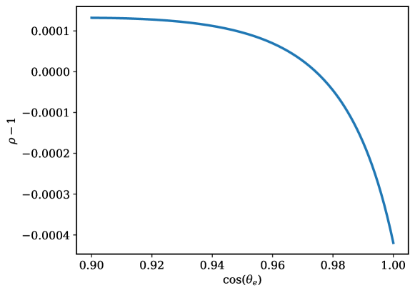
Figure 2: Ratio of the differential electron scattering rate for a ring and a point source. Assuming a fixed neutrino energy of 10 MeV and an opening angle of the ring of $\theta_{\text{sun}}$. The differences are at the sub-permil level.

In Fig. 2 we show the ratio

$$\rho=\frac{\displaystyle\operatorname{\text{d}}R_{r}/\operatorname{\text{d}}\Omega_{e}}{\displaystyle\operatorname{\text{d}}R_{p}/\operatorname{\text{d}}\Omega_{e}}\;.$$ (3.11)

That is the ratio of the differential rates for a ring and a point source. We used a fixed neutrino energy of 10 MeV and the opening angle of the ring is equivalent to the opening angle of the sun in the sky. For the cross section we also just consider electron neutrino electron scattering at this point. We see that it is not easy to distinguish the ring and the point source in this simplified setup. Their difference being only at the sub-permil level. That is actually not surprising considering the rather tiny opening angle of the ring compared to the typical scattering angle. The electron picture blurs such small neutrino pictures quite drastically at this energy.

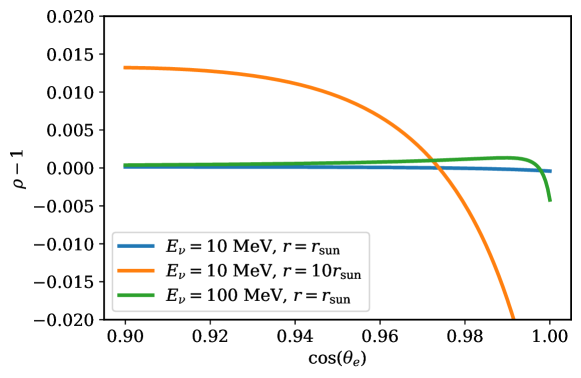
Figure 3: Ratio of the differential electron scattering rate for a ring and a point source. Assuming a fixed neutrino energy of 100 MeV and a ring with the radius of the sun and 10 MeV on the right with a ten times larger radius. The differences are at the percent level.

For comparison we also show the same ratio but change some of the parameters in Fig. 3. We first increase the neutrino energy to 100 MeV. The higher the neutrino energy the stronger the correlation between the electron and neutrino direction. Therefore the relative deviation grows in particular for small scattering angles and reaches the permil level.

Then we also increased the opening angle assuming a ring-like object which is ten times larger than the sun but again setting the neutrino energy to 10 MeV. We can see even deviations at the percent level also distributed over wider scattering angles which would make an experimental distinction between a point and a ring source significantly easier.

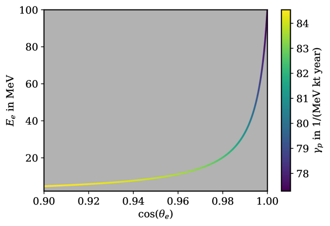
Figure 4: Representation of the double differential electron neutrino electron scattering rate in the $\cos\theta_{e}$-$E_{e}$ plane for a point source with a neutrino energy of 100 MeV and a neutrino flux of $5\times 10^{6}$ cm^-2 s^-1.

Nevertheless, we want to propose here not to look at the angular or energy rate distributions but at the double differential rate instead.

For a monochromatic point source this is not quite trivial since it is proportional to a $\delta$-function. Therefore we show in Fig. 4 the correlation between electron energy and scattering angle for a point source for a fixed neutrino energy of 100 MeV and the coefficient in front of the $\delta$-function, $\gamma_{p}$, c.f. eq. (3.2). In the grey areas there are no events for a monochromatic point source. We have assumed water as target material and a neutrino flux of $f_{0}=5\times 10^{6}$ cm^-2 s^-1. While the flux corresponds roughly to the solar ⁸B neutrino flux we have increased the neutrino energy to values larger than typical solar neutrinos to show more clearly the difference to a ring source in that same plane.

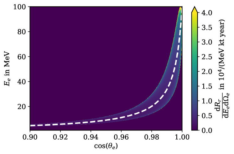
Figure 5: Double differential scattering rate for a ring source. We assume a fixed neutrino energy of 100 MeV, a neutrino flux of $5\times 10^{6}$ cm^-2 s^-1 and the ring is ten times larger than the sun for better visibility. For comparison we show as a white dashed line the correlation between electron energy and scattering angle for a point source, cf. Fig. 4. To increase the visibility of the extremely thin distribution we cap the color scale at $4\times 10^{4}$ 1/(MeV kt year).

We show that difference in Fig. 5 where we plot the double differential rate for a ring source ten times the size of the sun and a neutrino energy of 100 MeV for water as target material. For a comparison we show the line for a 100 MeV point source. We can see that the ring in the two-dimensional plane looks clearly different from a point source. Interestingly the event rates get larger towards the outside of the distribution which might be possible to be exploited experimentally.

Nevertheless, this have all been toy examples so far. In a realistic source the geometry is usually not simple and also very often the neutrino energy is not fixed to a concrete value.

3.2 Towards Realistic Pictures

Before going to the full pictures we want to study one intermediate step first. We will again compare a ring and a point source, but use the energy distribution, total flux and flavour information as expected for ⁸B neutrinos which are most well studied in water Cherenkov detectors.

Starting again from our key formula, eq. (2.13), we can find the double differential rate for a point source with ⁸B energy spectrum

$$\frac{\operatorname{\text{d}}R^{p}_{\text{8B}}}{\operatorname{\text{d}}E_{e}\operatorname{\text{d}}\Omega_{e}} =\frac{N_{e}\,f_{0}^{\text{8B}}}{2\pi\,M_{D}}\frac{\operatorname{\text{d}}\epsilon_{\text{8B}}}{\operatorname{\text{d}}E_{\nu}}(E_{\nu}^{p})\frac{\operatorname{\text{d}}\sigma(E_{e},E_{\nu}^{p})}{\operatorname{\text{d}}E_{e}}m_{e}\left|\frac{(E_{e}-m_{e})\sqrt{E_{e}^{2}-m_{e}^{2}}}{(E_{e}-m_{e}-\cos\theta_{e}\sqrt{E_{e}^{2}-m_{e}^{2}})^{2}}\right|\;,$$ (3.12)

where

$$E_{\nu}^{p}=\frac{m_{e}(E_{e}-m_{e})}{m_{e}-E_{e}+\cos\theta_{e}\sqrt{E_{e}^{2}-m_{e}^{2}}}\;.$$ (3.13)

For a ring source with ⁸B energy spectrum we find

$$\frac{\operatorname{\text{d}}R^{r}_{\text{8B}}}{\operatorname{\text{d}}E_{e}\operatorname{\text{d}}\Omega_{e}} =\frac{N_{e}\,f_{0}^{\text{8B}}}{4\pi^{2}\,M_{D}}\int_{0}^{2\pi}\operatorname{\text{d}}\phi_{\nu}\frac{\operatorname{\text{d}}\epsilon_{\text{8B}}}{\operatorname{\text{d}}E_{\nu}}(E_{\nu}^{r})\frac{\operatorname{\text{d}}\sigma(E_{e},E_{\nu}^{r})}{\operatorname{\text{d}}E_{e}}$$

$$\phantom{\frac{N_{e}\,f_{0}^{\text{8B}}}{4\pi^{2}\,M_{D}}\int_{0}^{2\pi}\operatorname{\text{d}}\phi_{\nu}\frac{\operatorname{\text{d}}\epsilon_{\text{8B}}}{\operatorname{\text{d}}E_{\nu}}(E_{\nu}^{r})}\times m_{e}\left|\frac{(E_{e}-m_{e})\sqrt{E_{e}^{2}-m_{e}^{2}}}{(E_{e}-m_{e}-(\hat{p}_{\nu}\cdot\hat{q}_{e})_{r}\sqrt{E_{e}^{2}-m_{e}^{2}})^{2}}\right|\;,$$ (3.14)

where

$$E_{\nu}^{r} =\frac{m_{e}(E_{e}-m_{e})}{m_{e}-E_{e}+(\hat{p}_{\nu}\cdot\hat{q}_{e})_{r}\sqrt{E_{e}^{2}-m_{e}^{2}}}\;,$$ (3.15)

$$(\hat{p}_{\nu}\cdot\hat{q}_{e})_{r} =\sqrt{1-c_{r}^{2}}\cos\phi_{\nu}\cos\phi_{e}\sin\theta_{e}+\sqrt{1-c_{r}^{2}}\sin\phi_{\nu}\sin\phi_{e}\sin\theta_{e}+c_{r}\cos\theta_{e}\;.$$ (3.16)

More details on how to derive these formulas are given in App. B. For the energy distribution we take in both cases the GS98 prediction taken from [27] with $f_{0}^{\text{8B}}=5.46\times 10^{6}$ cm^-2 s^-1.

We will also include neutrino oscillations into the picture at this point. As long as we consider elastic neutrino electron scattering $\mu$- and $\tau$-neutrinos are indistinguishable, but the cross section is different for them compared to electron neutrinos. To deal with this we will replace the differential cross section in the above formulas with

$$\frac{\operatorname{\text{d}}\sigma(E_{e},E_{\nu})}{\operatorname{\text{d}}E_{e}}=P_{ee}(E_{\nu})\frac{\operatorname{\text{d}}\sigma(\nu_{e}e\to\nu_{e}e)}{\operatorname{\text{d}}E_{e}}+(1-P_{ee}(E_{\nu}))\frac{\operatorname{\text{d}}\sigma(\nu_{l}e\to\nu_{l}e)}{\operatorname{\text{d}}E_{e}}\;,$$ (3.17)

where we have introduced the electron neutrino survival probability for electron neutrinos produced in the sun, which is generally energy dependent. For simplicity, we will nevertheless use the constant value $P_{ee}=0.37$ [28] as an approximation since the energy dependence is not very strong in the considered range.

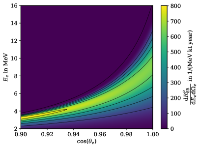
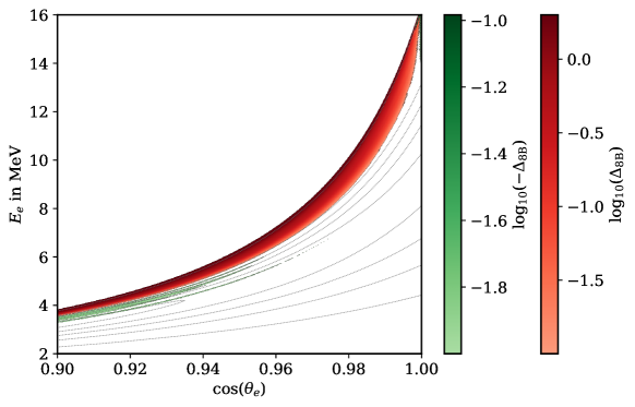
Figure 6: On top we show the double differential rate for neutrinos with energy spectrum as the solar ⁸B neutrinos have. On the top left we assume the neutrinos are produced in a point at the center of the sun and on the top right we assume they are produced in a ring the size of the sun. On the bottom we show the relative difference $\Delta_{\text{8B}}$ for the double differential event rates between a point source and a ring source the size of the sun using otherwise identical parameters. In the white regions the absolute, relative difference is either less than 1 % or not well-defined. In the red shaded regions the ring source would lead to more events while in the green regions the point source would result in more events. For easier comparison we show the contour lines of the point source in the comparison plot as dotted lines.

In Fig. 6 we first show the double differential distribution in this setup for the point and the ring source on top. Although we are considering a point source here on the top left the double differential distribution is not a line at all which is due to the continuous energy distribution. The case for a ring the size of the sun is extremely similar to the point source and hard to distinguish by eye.

We therefore defined the ratio

$$\Delta_{\text{8B}}=\frac{\displaystyle\frac{\operatorname{\text{d}}R^{r}_{\text{8B}}}{\operatorname{\text{d}}E_{e}\operatorname{\text{d}}\Omega_{e}}-\frac{\operatorname{\text{d}}R^{p}_{\text{8B}}}{\operatorname{\text{d}}E_{e}\operatorname{\text{d}}\Omega_{e}}}{\displaystyle\frac{1}{2}\left(\frac{\operatorname{\text{d}}R^{r}_{\text{8B}}}{\operatorname{\text{d}}E_{e}\operatorname{\text{d}}\Omega_{e}}+\frac{\operatorname{\text{d}}R^{p}_{\text{8B}}}{\operatorname{\text{d}}E_{e}\operatorname{\text{d}}\Omega_{e}}\right)}\;,$$ (3.18)

which is the difference of the two cases normalised by their average. The result for $\log_{10}|\Delta_{\text{8b}}|$ is also shown in Fig. 6. In the white regions $|\Delta_{\text{8b}}|$ is either less than 1 % or not well-defined. The biggest difference is actually at the edge of the distributions, which can be easily explained. For a ring source we expect to still see events for larger scattering angles at the same electron energy since a larger source will result in a larger picture. But the region where this difference is significant is unfortunately quite small and also where the absolute event rate is not that large.

4 Neutrino Pictures of the Sun via Electrons

So far we have discussed only point and ring sources. Realistic solar models predict neither. In this section we will discuss the fully realistic case for ⁸B, hep and pep neutrinos. These three neutrino sources are dominantly produced in different regions of the sun. The ⁸B neutrinos are being produced more towards the center of the sun while hep and pep neutrinos have the peak production zone more outwards. We choose these three sources for our benchmark study, not only because they are well separated in the sun, but also due to the fact that they have different features in energy. The hep neutrinos can reach up to $19$ MeV which is the highest one among the three, and are expected to be identified by HyperK [19]. However, for pep neutrinos the energy is constant at $1.445$ MeV. By taking proper energy cuts, we can separate them from each other.

4.1 Angular Distributions from Radial Production Zones

We begin the discussion with deriving the normalised neutrino luminosity profile of the sun from radial production zones. There have been many works studying solar models and in our calculations we will use the results from [29]. For the considered neutrino fluxes the results between the various calculations are usually similar.

What they usually provide in the literature are tables of the amount of neutrinos produced in a given radial shell, i.e., they provide a discrete version of a function $\operatorname{\text{d}}j/\operatorname{\text{d}}\zeta$, where $\zeta=r/r_{\text{sun}}$. That implies $\operatorname{\text{d}}j/\operatorname{\text{d}}r=r_{\text{sun}}\operatorname{\text{d}}j/\operatorname{\text{d}}\zeta$. In our codes we import these data sets, interpolate and normalise them such that

$$\int_{0}^{1}\frac{\operatorname{\text{d}}j}{\operatorname{\text{d}}\zeta}\operatorname{\text{d}}\zeta=\int_{0}^{r_{\text{sun}}}\frac{\operatorname{\text{d}}j}{\operatorname{\text{d}}r}\operatorname{\text{d}}r=1\;.$$ (4.1)

Note that here it is implicitly assumed that the production zones are spherically symmetric, i.e., they only depend on the radius. That also implies that the normalised neutrino production rate per unit volume at any given point is given by

$$J(\vec{r})=\frac{1}{4\,\pi\,r^{2}}\frac{\operatorname{\text{d}}j}{\operatorname{\text{d}}r}\;.$$ (4.2)

On earth we can of course just observe a two-dimensional projection of the neutrino production distribution, which we can calculate using the line of sight integral

$$\frac{\operatorname{\text{d}}\lambda(\theta_{\nu},\phi_{\nu})}{\operatorname{\text{d}}\Omega_{\nu}}=\mathcal{N}_{\lambda}\int\operatorname{\text{d}}l\;J(\vec{l})\;,$$ (4.3)

where $l$ parametrises the line of sight and for convenience we introduce the normalisation constant $\mathcal{N}_{\lambda}$ such that

$$\int\frac{\operatorname{\text{d}}\lambda}{\operatorname{\text{d}}\Omega_{\nu}}\operatorname{\text{d}}\Omega_{\nu}=1\;.$$ (4.4)

Here we assumed that neutrinos just travel undisturbed through the sun neglecting any attenuation and scattering effects in the sun for simplicity and we have already mentioned how we treat neutrino oscillations.

The observed total neutrino flux on earth is then given by

$$F=f_{0}\int\operatorname{\text{d}}E_{\nu}\int\operatorname{\text{d}}\Omega_{\nu}\frac{\operatorname{\text{d}}\epsilon}{\operatorname{\text{d}}E_{\nu}}\frac{\operatorname{\text{d}}\lambda}{\operatorname{\text{d}}\Omega_{\nu}}$$ (4.5)

Note that we integrate here the absolute value of the flux over the source. We do not take the scalar product of the flux with an arbitrary detector area first and then integrate over the source. That would lead to different values for the flux, especially for large, extended sources. For the sun, the difference is not that large and we want to focus here on distributions and ignore this subtle normalisation issue. We always specify what value of $f_{0}$ we choose when needed.

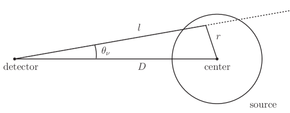
Figure 7: We assume a radial symmetric source and a point-like detector. Taking the line of sight integral we get the two-dimensional luminosity profile of the source.

The problem in the derivation of the angular distribution is that we cannot directly use eq. (4.3) since we do not have the function $J(\vec{l})$ or $\operatorname{\text{d}}j(l)/\operatorname{\text{d}}l$ readily available. We only have the luminosity profile as a function of the normalised distance from the centre of the sun, i.e., we have $\operatorname{\text{d}}j(\zeta)/\operatorname{\text{d}}\zeta$ or $r_{\text{sun}}\operatorname{\text{d}}j(r)/\operatorname{\text{d}}r$.

From basic geometry, cf. Fig. 7, we know that

$$r^{2} =D^{2}+l^{2}-2\,D\,l\cos\theta_{\nu}\;,$$ (4.6)

$$\Rightarrow r\operatorname{\text{d}}r =(l-D\cos\theta_{\nu})\operatorname{\text{d}}l\;,$$ (4.7)

where $D$ is the distance between the observer and the center of the sun. For future reference, we also note here that the maximum observation angle for a finite, radial symmetric source where the source center is at $\theta_{\nu}=0$ is given by

$$\cos\theta_{\nu}^{\text{max}}=\sqrt{1-\frac{r_{\text{sun}}^{2}}{D^{2}}}\;.$$ (4.8)

We can now use the two solutions for $l(r)$

$$l(r)=\begin{cases}l_{1}(r)=D\cos\theta_{\nu}-\sqrt{r^{2}+\frac{D^{2}}{2}(\cos(2\theta_{\nu})-1)}\text{ for }l\leq D\cos\theta_{\nu}\;,\\ l_{2}(r)=D\cos\theta_{\nu}+\sqrt{r^{2}+\frac{D^{2}}{2}(\cos(2\theta_{\nu})-1)}\text{ for }l>D\cos\theta_{\nu}\;.\end{cases}$$ (4.9)

The minimal and maximal line of sight are here

$$l_{\text{max/min}}\equiv D\cos\theta_{\nu}\pm\sqrt{r_{\text{sun}}^{2}+\frac{D^{2}}{2}(\cos(2\theta_{\nu})-1)}\;.$$ (4.10)

We can then write

$$\frac{\operatorname{\text{d}}\lambda(\theta_{\nu},\phi_{\nu})}{\operatorname{\text{d}}\Omega_{\nu}} =\mathcal{N}_{\lambda}\int_{l_{\text{min}}}^{l_{\text{max}}}\operatorname{\text{d}}l\;J(\vec{l})$$

$$=\mathcal{N}_{\lambda}\int_{l_{\text{min}}}^{D\cos\theta_{\nu}}\operatorname{\text{d}}l_{1}\;J(\vec{l}_{1})+\mathcal{N}_{\lambda}\int_{D\cos\theta_{\nu}}^{l_{\text{max}}}\operatorname{\text{d}}l_{2}\;J(\vec{l}_{2})$$

$$=\mathcal{N}_{\lambda}\int_{r_{\text{sun}}}^{D\sin\theta_{\nu}}\frac{r\,\operatorname{\text{d}}r}{l_{1}(r)-D\cos\theta_{\nu}}\;\frac{1}{4\,\pi\,r^{2}}\frac{\operatorname{\text{d}}j(r)}{\operatorname{\text{d}}r}$$

$$\phantom{=}+\mathcal{N}_{\lambda}\int_{D\sin\theta_{\nu}}^{r_{\text{sun}}}\frac{r\,\operatorname{\text{d}}r}{l_{2}(r)-D\cos\theta_{\nu}}\;\frac{1}{4\,\pi\,r^{2}}\frac{\operatorname{\text{d}}j(r)}{\operatorname{\text{d}}r}$$

$$=\frac{\mathcal{N}_{\lambda}}{2\,\pi}\int_{D\sin\theta_{\nu}}^{r_{\text{sun}}}\frac{\operatorname{\text{d}}r}{r\sqrt{r^{2}-D^{2}\sin^{2}\theta_{\nu}}}\frac{\operatorname{\text{d}}j(r)}{\operatorname{\text{d}}r}$$

$$=\frac{\mathcal{N}_{\lambda}}{2\,\pi\,r_{\text{sun}}^{2}}\int^{1}_{D\sin\theta_{\nu}/r_{\text{sun}}}\frac{\operatorname{\text{d}}\zeta}{\zeta\sqrt{\zeta^{2}-(D/r_{\text{sun}})^{2}\sin^{2}\theta_{\nu}}}\frac{\operatorname{\text{d}}j(\zeta)}{\operatorname{\text{d}}\zeta}\;.$$ (4.11)

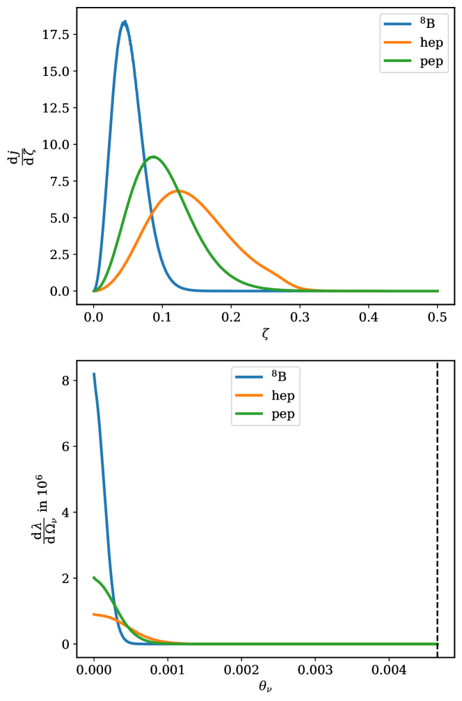
Figure 8: The normalised radial neutrino ⁸B, hep and pep production rate as a function of $\zeta=r/r_{\text{sun}}$ taken from the GS98 composition of [29] on top and the resulting angular distribution as a function of $\theta_{\nu}$ on the bottom. Note that we assume a radial symmetric distribution. The dashed vertical line in the plot on the bottom denotes the optical size of the sun.

The resulting distributions together with the original radial distributions for the ⁸B, the hep and the pep flux are shown in Fig. 8.

The most well experimentally studied neutrinos, the ⁸B neutrinos are concentrated very much in the center of the sun. While the optical angular diameter of the sun in the sky is about 0.5^∘ it is just about 0.07^∘ for the ⁸B neutrinos and resolving them is certainly a challenge. At this point we would like to comment on the result in [18]. From their Fig. 1 we have the impression that their underlying neutrino angular distribution has a peak at $\cos\theta_{\nu}<1$ since their electron angular distribution peaks at $\cos\theta_{e}\approx 0.984<1$. In our case, both neutrino and electron angular distribution peak at the center of the sun. We will come back to this point later.

The hep and the pep neutrinos are somewhat better to resolve as their distributions are about two to three times wider than the ⁸B neutrino one leading to production zones with a diameter of about 0.14^∘ which is nevertheless still small.

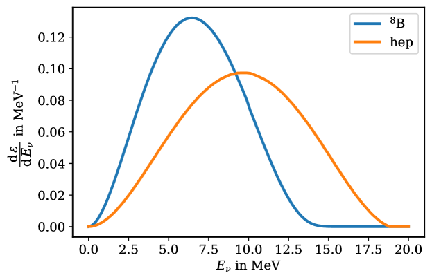
Figure 9: The normalised solar neutrino energy spectrum for ⁸B and hep neutrinos taken from [27]. For the hep neutrinos we take the average of the two data sets provided there.

As a reminder before we continue, the energy distribution of the produced neutrinos is to a good approximation independent from the production zone and we will use the energy distributions from [27]. For completeness and convenience of the reader we show the normalised ⁸B and hep energy distributions in Fig. 9. The pep neutrinos are monochromatic with a neutrino energy $E_{\nu}^{\text{pep}}=1.445$ MeV.

4.2 ⁸B Neutrinos

At this point we have all the basic ingredients collected to discuss how we expect the ⁸B neutrinos from the sun look via electrons.

We again begin with the double differential event rate

$$\frac{\operatorname{\text{d}}R_{\text{8B}}}{\operatorname{\text{d}}E_{e}\operatorname{\text{d}}\Omega_{e}} =\frac{N_{e}\,f_{0}^{\text{8B}}}{2\pi\,M_{D}}\int\operatorname{\text{d}}\Omega_{\nu}\frac{\operatorname{\text{d}}\epsilon_{\text{8B}}}{\operatorname{\text{d}}E_{\nu}}(\bar{E}_{\nu})\frac{\operatorname{\text{d}}\sigma}{\operatorname{\text{d}}E_{e}}(E_{e},\bar{E}_{\nu})\frac{\operatorname{\text{d}}\lambda_{\text{8B}}(\Omega_{\nu})}{\operatorname{\text{d}}\Omega_{\nu}}$$

$$\phantom{=\frac{N_{e}\,f_{0}^{\text{8B}}}{2\pi\,M_{D}}\int\operatorname{\text{d}}\Omega_{\nu}}\times\frac{\bar{E}_{\nu}\,\sqrt{E_{e}^{2}-m_{e}^{2}}}{|\hat{p}_{\nu}\cdot\hat{q}_{e}\sqrt{E_{e}^{2}-m_{e}^{2}}-(E_{e}-m_{e})|}\;,$$ (4.12)

with

$$\bar{E}_{\nu}=\frac{m_{e}(E_{e}-m_{e})}{\hat{p}_{\nu}\cdot\hat{q}_{e}\sqrt{E_{e}^{2}-m_{e}^{2}}-(E_{e}-m_{e})}$$ (4.13)

and

$$\hat{p}_{\nu}\cdot\hat{q}_{e}=\sin\theta_{\nu}\cos\phi_{\nu}\cos\phi_{e}\sin\theta_{e}+\sin\theta_{\nu}\sin\phi_{\nu}\sin\phi_{e}\sin\theta_{e}+\cos\theta_{\nu}\cos\theta_{e}\;.$$ (4.14)

The remaining integration over $\Omega_{\nu}$ is highly non-trivial and has to be evaluated numerically. For some comments on the derivation of these formulas we refer to App. B.4. The energy distribution and flux factor $f_{0}^{\text{8B}}=5.46\times 10^{6}$ cm^-2 s^-1 is the GS98 result from [27].

Like in the previous section we will also use here a constant electron neutrino survival probability $P_{ee}=0.37$ [28] and use for the differential cross section in the above formula

$$\frac{\operatorname{\text{d}}\sigma(E_{e},E_{\nu})}{\operatorname{\text{d}}E_{e}}=P_{ee}(E_{\nu})\frac{\operatorname{\text{d}}\sigma(\nu_{e}e\to\nu_{e}e)}{\operatorname{\text{d}}E_{e}}+(1-P_{ee}(E_{\nu}))\frac{\operatorname{\text{d}}\sigma(\nu_{l}e\to\nu_{l}e)}{\operatorname{\text{d}}E_{e}}\;.$$ (4.15)

Figure 10: Double differential distribution of electrons recoiling from scattering with solar ⁸B neutrinos for a water Cherenkov detector. We show the distribution for $\phi_{e}=0$.

In Fig. 10 we show the double differential rate in the $\cos\theta_{e}$-$E_{e}$ plane. We see that this picture is hard to distinguish from the case of the point or ring source shown in Fig. 6 since the distribution is extremely narrow in the sky. Again the structure here is a non-trivial overlay of different neutrino energies originating from different places within the sun. Although the dominant part is clearly coming from the fact that for a given scattering angle different neutrino energies contribute with different cross sections and hence rate which is folded with how likely that energy is.

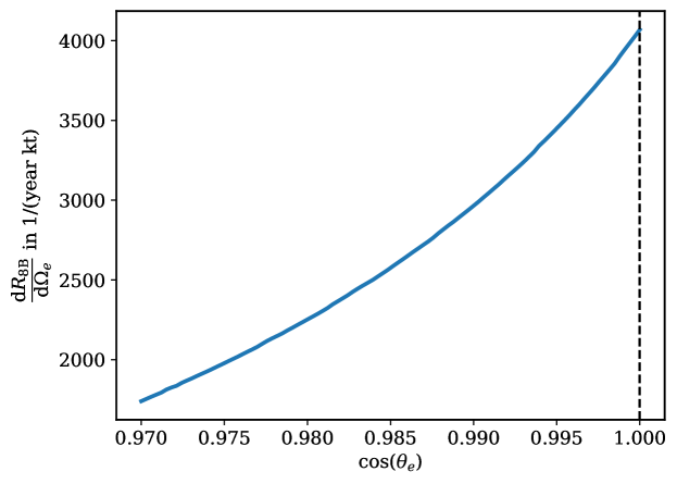
Figure 11: Angular distribution of electrons scattered by solar ⁸B neutrinos for a water Cherenkov detector. We show the distribution for $\phi_{e}=0$ and stress that the distribution is independent of $\phi_{e}$. We integrated the electron recoil energy from $T_{e}=3.5$ MeV to the maximally possible energy. The dashed vertical line in the plot denotes the optical size of the sun.

We like to briefly comment on the angular distribution more often seen in the literature. We show such a distribution in Fig. 11, which is obtained by integrating eq. (4.12) over the electron energy. The event number in this figure is calculated with respect to the Super-Kamiokande detector, i.e., a kinetic energy threshold $T_{e}\geq 3.5$ MeV, cf. [30], is taken for the water target. Since the distribution is radially symmetric, it is sufficient to plot it for a fixed value of $\phi_{e}=0$.

What we see here is a rather featureless distribution which has its maximum at $\cos\theta_{e}=1$ and then smoothly falls for smaller values of $\cos\theta_{e}$ which agrees, for instance, with the data shown in [31]. This distribution should be equivalent to the distribution shown in Fig. 1 of [18] apart from using different units. While they obtain a pronounced peak at $\cos\theta_{e}\approx 0.984$ we do not find such a peak in our results. We checked that this remains true also if we use the higher threshold of $T_{e}=5$ MeV of [18]. Nevertheless, we can understand our result as the peak of the electron angular distribution falls together with the peak of the neutrino luminosity distribution. Unfortunately, [18] does not show the assumed angular distribution of neutrino luminosity, which would be very useful for comparison. It might also be that they included energy dependent efficiency factors and other uncertainties, which we do not know at this point.

4.3 hep Neutrinos

The second example we like to discuss is the double differential rate of the so-called hep neutrinos. Compared to ⁸B neutrinos, hep neutrinos can reach a higher maximal energy, which is almost $19$ MeV while the maximal energy of ⁸B neutrinos is about 16 MeV. The hep neutrinos are less studied experimentally because their flux is rather suppressed compared to that of ⁸B neutrinos. The GS98 prediction for the flux of hep neutrinos is $0.8\times 10^{4}$ cm^-2 s^-1 compared to $5.46\times 10^{6}$ cm^-2 s^-1 for the ⁸B neutrinos [27].

So apart from the magnitudes and spectral shapes of the fluxes, the physics for ⁸B and hep neutrinos is essentially the same and we shall use the same formulas as in the previous section. To be specific, we take $f_{0}^{\text{hep}}=0.8\times 10^{4}$ cm^-2 s^-1. The production zones of hep neutrinos are taken from [29] resulting in the angular distribution derived at the beginning of this section, cf. Fig. 8, and for the energy distribution we use the average of the quoted minimum and maximum from [27] and normalise the distribution. The interaction cross section between hep neutrinos and electrons is taken to be the same as the one in the case of ⁸B neutrinos.

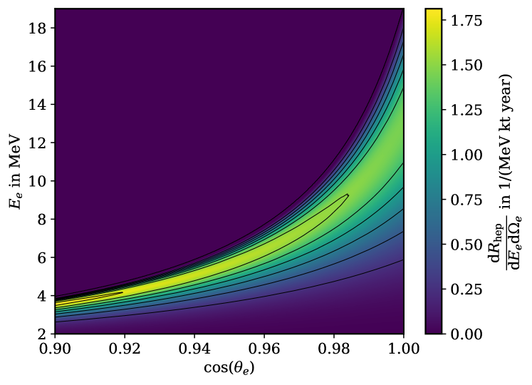
Figure 12: Double differential distribution of electrons recoiling from scattering with solar hep neutrinos for a water Cherenkov detector. We show the distribution for $\phi_{e}=0$.

We then find for the double differential distribution the result shown in Fig. 12. Not surprisingly, shapes of the contours resemble those of ⁸B. The most notable differences is the larger possible electron energies and the much lower event rate compared to ⁸B.

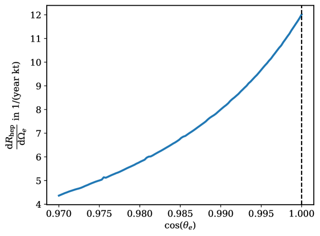
Figure 13: Angular distribution of electrons scattered by solar hep neutrinos for a water Cherenkov detector. We show the distribution for $\phi_{e}=0$ and stress that the distribution is independent of $\phi_{e}$. We integrated the electron recoil energy from $T_{e}=3.5$ MeV to the maximally possible energy. The dashed vertical line in the plot denotes again the optical size of the sun.

We also show the angular distribution for hep neutrinos in Fig. 13. As before for the ⁸B neutrinos, cf. Fig. 11 the distribution is very featureless. The small bumps are due to numerics and do not correspond to any identifiable physical features. That is also consistent with our expectations as discussed before.

4.4 pep Neutrinos

The third example we like to discuss is the so-called pep neutrinos. Different from ⁸B and hep neutrinos, pep neutrinos are monochromatic. In principle, this could make the reconstruction of source geometry easier.

On the other hand it is quite challenging to detect pep neutrinos due to their relatively low energy of only $E_{\nu}^{\text{pep}}=1.445$ MeV, although their total flux on Earth is not very small. The GS98 prediction gives $f_{0}^{\text{pep}}=1.44\times 10^{8}$ cm^-2 s^-1 [27], which is significantly larger than the ⁸B neutrino flux.

Again we just quote here the results for the distributions of the event rate and refer the interested reader to App. B.4 for a detailed derivation. For the double differential rate we find

$$\frac{\operatorname{\text{d}}R_{\text{pep}}}{\operatorname{\text{d}}E_{e}\operatorname{\text{d}}\Omega_{e}} =\frac{N_{e}\,f_{0}^{\text{pep}}}{\pi\,M_{D}}\frac{\operatorname{\text{d}}\sigma(E_{e},E_{\nu}^{\text{pep}})}{\operatorname{\text{d}}E_{e}}\int\operatorname{\text{d}}\cos\theta_{\nu}\frac{\operatorname{\text{d}}\lambda_{\text{pep}}(\cos\theta_{\nu})}{\operatorname{\text{d}}\Omega_{\nu}}\,$$

$$\quad\times\left(\sin^{2}\theta_{\nu}\,\sin^{2}\theta_{e}-\left(\frac{(E_{e}-m_{e})(E_{\nu}^{\text{pep}}+m_{e})}{E_{\nu}^{\text{pep}}\,\sqrt{E_{e}^{2}-m_{e}^{2}}}-\cos\theta_{e}\cos\theta_{\nu}\right)^{2}\right)^{-\tfrac{1}{2}}\;.$$ (4.16)

So we are just left with the integration over $\cos\theta_{\nu}$, which has to be evaluated numerically. To obtain only the physical solution, we have to ensure that the term under the square root remains positive.

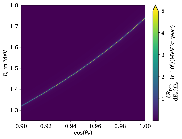
Figure 14: Double differential distribution of electrons recoiling from scattering with solar pep neutrinos. We show the distribution for $\phi_{e}=0$. To increase the visibility of the extremely thin distribution we cap the color scale at $5\times 10^{6}$ 1/(MeV kt year).

We show the resulting double differential rate in Fig. 14. As expected from what we have seen in Sec. 3 and taking into account the rather low neutrino energy and narrow angular distribution, the distribution looks quite similar to a line although it has a finite width. Resolving this in an experiment might be quite challenging. On the other hand, this strong correlation could be exploited to distinguish a pep neutrino signal from background sources.

Since the pep signal is below typical thresholds for water Cherenkov detectors, we do not show the angular distribution of the event rate here.

5 Impacts of Angular and Energy Uncertainties in Experiments

So far we have treated everything from a purely theoretical viewpoint. Particularly, we have not included reconstruction uncertainties in energies and directions of electrons. Such uncertainties lead to an additional blurring of the picture. One would also need to consider how experimental errors affect the Radon transform which allows the reconstruction of the neutrino image from electron data, cf. Sec. 2, which we leave for future works.

To illustrate the impact of experimental uncertainties, we assume in this section a very simple Gaussian error model for the reconstructed energy in the detector, $E_{d}$, and direction $\hat{q}_{d}$. Following [14], we assume that the above two uncertainties are independent from each other. Hence the reconstructed double differential rate is given by

$$\frac{\operatorname{\text{d}}R}{\operatorname{\text{d}}E_{d}\operatorname{\text{d}}\Omega_{d}}=\int\operatorname{\text{d}}E_{e}\operatorname{\text{d}}\Omega_{e}\frac{\operatorname{\text{d}}R}{\operatorname{\text{d}}E_{e}\operatorname{\text{d}}\Omega_{e}}f_{E}(E_{e},E_{d},\sigma_{E})f_{\theta}(\Omega_{e},\Omega_{d},\sigma_{\theta})\;.$$ (5.1)

The functions $f_{E}$ and $f_{\theta}$ are Gaussian error functions given by

$$f_{E}=\mathcal{N}_{E}\exp\left(-\frac{(E_{e}-E_{d})^{2}}{2\,\sigma_{E}^{2}}\right)\;,$$ (5.2)

$$f_{\theta}=\mathcal{N}_{\theta}\exp\left(-\frac{\arccos^{2}(\hat{q}_{e}\cdot\hat{q}_{d})}{2\,\sigma_{\theta}^{2}}\right)\;,$$ (5.3)

where $\mathcal{N}_{E}$, $\mathcal{N}_{\theta}$ are normalisation constants, for more details, see App. C. We want to stress here that this is strongly simplified and should only serve some simple illustrative purposes to see, if experimental uncertainties have the tendency to make the distinction between different images more difficult.

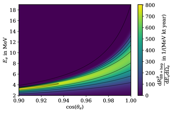
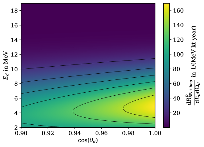
Figure 15: The double differential rate for a point source with ⁸B and hep neutrino fluxes. On top we show the original distribution while on the bottom we show the distribution after the inclusion of simplified experimental smearing. We show the distributions for $\phi_{e/d}=0$.

We then calculated the double differential rate after doing this additional smearing, see Fig. 15, where we assumed a point source and included ⁸B and hep neutrino fluxes. For an immediate comparison, we show both double differential distributions before and after smearing in the plot. For the energy resolution we assumed $\sigma_{E}=1.5$ MeV and for the angular resolution we have set $\sigma_{\theta}=20^{\circ}$ which are typical numbers for a water Cherenkov detector, cf. [32]. We note that the hep neutrino contribution is hard to see by comparing this result to Fig. 10. It is not surprising since hep neutrino flux and hence the expected rate is so much lower than the ⁸B component, cf. Fig. 12, despite that the hep neutrino contribution dominates for electron energies beyond 16 MeV.

The smeared distribution looks substantially different from the original picture which is not surprising. The horizontal axis corresponds to a range for $\theta_{d}$ of about 0^∘-26^∘. So it is not even two $\sigma_{\theta}$ wide. The smearing due to the energy resolution on the other hand is comparatively small. Hence, we consider it more urgent to improve the angular resolution should one want to resolve structures in the neutrino picture of the sun.

To understand this prospects better we also computed for comparison the smeared distribution for a ring source the size of the sun and compared it to the displayed point source, as we did in Sec. 3.1. Nowhere in the displayed region we found a difference between the two distributions larger than 1%, which is different from comparing two sources without taking into account the smearing. Therefore we expect that experimental uncertainties can blur the neutrino images as we have seen here. In fact the detection efficiency due to event selection cuts will reduce the statistics and consequently further blur the neutrino images. We leave detailed considerations such as the above for future publications.

Similar to Sec. 4, one can calculate the double differential rate for a realistic ⁸B neutrino source with smearing effects considered. However, it is not particularly illuminating to show the result here since it is not visually distinguishable from the result of a point source.

At this point one might dismiss our exercise here as unfeasible. In fact, it seems far fetched to measure structures which are smaller than 0.1^∘ with an instrument which has a 20^∘ resolution. But this is a bit too simplistic since the 20^∘ resolution applies to an individual electron measurement. Would we suppose all electrons come from a single point source and the error is Gaussian we could determine the position of the source with a resolution $\sigma_{\theta}/\sqrt{N_{\text{evt}}}$, where $N_{\text{evt}}$ is the event number. Super-Kamiokande reported about 1000 solar neutrino events in phase IV [31] which would lead to a naive angular resolution of the right order. Similar arguments were used in [18]. Hence, in the future with significantly increased statistics it might be possible to provide an upper bound on the size of the sun in neutrinos even without improving the angular resolution for an individual event drastically.

We also want to remind here, that we just use solar neutrinos as a well understood template for our formalism and that other sources which are larger and/or have higher energies might fare better. One of us, for instance, discussed a hypothetical neutrino signature from DM annihilation in the Earth’s core [33]. There they found that for DM mass as heavy as $10^{4}$ GeV, the muon-track resolution in IceCube and the size of the neutrino production zone are both around 1^∘. To image such a neutrino production zone, it is necessary to calculate angular distributions of muons resulting from deep inelastic neutrino-nucleon scatterings. Such a calculation is however beyond the scope of the current work [34].

6 Summary and Conclusions

In this article we have investigated how one could take a neutrino “picture” by studying the energy and angular distributions of elastically scattered electrons. We show how the electron distributions are related to the original neutrino distributions and also briefly mention how this relation can be inverted. These formulas are in fact strongly inspired by the formalism developed for directional dark matter searches. However the formalism here is more involved due to the relativistic nature of the incoming neutrinos.

We have applied our formalism first to simple toy examples where we fixed the neutrino energy and assumed the source to be either point- or ring-like. These are two extreme cases and we have discussed how much they differ in the angular and the double differential rate distributions. Assuming a neutrino energy spectrum similar to that of ⁸B solar neutrinos, we have seen that the difference of the double differential rate for a point and a ring source could be up to a few percent. On the other hand, this occurs in regions where the event rate is rather low making such a distinction rather challenging.

We have chosen solar neutrinos here, since they are among the most well-studied extended neutrino sources where there is not only significant amount of experimental data but also elaborated theoretical calculations predicting the neutrino production rates within the solar layers. These theoretical predictions can be turned into an angular neutrino luminosity distribution which together with the predicted energy spectrum and scattering cross sections were then translated by us into neutrino pictures of the sun seen via electrons. We did this for the dominant ⁸B and hep neutrinos and also commented on the pep neutrinos and remind that they are produced in different regions of the sun. By comparing double differential event rates for these neutrinos, we found the specific ranges of electron energy for different sources. Although the events of hep neutrinos are not copious, they could be distinguished from ⁸B neutrinos by taking an energy cut at $E_{e}\sim 16$ MeV. It is expected that hep neutrinos will be identified by the HyperK experiment. The pep neutrinos are interesting because they are monochromatic. However, their energy is too low for them to be detected by current and upcoming water Cherenkov detectors which is our focus in this paper.

Uncertainty in reconstructing the electron direction is unfortunately not small. Hence, we also studied how a simple error model would affect the picture and the difference between a point and a ring source for a combined ⁸B and hep energy flux. As one might have expected, the difference is washed out by our simplified consideration of experimental uncertainties.

We envisage that the understanding of the solar model will be improved with the measurement of hep and pep neutrinos by HyperK and other future neutrino experiments. Our results stress the importance of future improvements in event statistics, energy resolutions, and angular resolutions.

In conclusion, we have established a theoretical framework for relating the neutrino image to an image of scattered particles which can be measured directly. This framework is not exclusively limited to solar neutrinos but can be applied to all kinds of extended neutrino sources such as, for instance, geoneutrinos, lunar neutrinos, neutrinos from DM interactions in various settings, atmospheric and solar atmospheric neutrinos or neutrinos from the galactic center just to name a few possibilities. Our work is applicable to all these cases should one like to reconstruct the neutrino picture taken via any charged leptons or hadrons.

Appendix A Elastic Neutrino Electron Scattering Cross Sections

For the convenience of the reader we quote here the differential elastic neutrino electron scattering cross section which we use throughout the paper taken from [26] rewritten in terms of $E_{e}$

$$\frac{\operatorname{\text{d}}\sigma(\nu_{\alpha}e\to\nu_{\alpha}e)}{\operatorname{\text{d}}E_{e}} =\frac{2\,G_{\mu}^{2}m_{e}}{\pi}\left[g_{\alpha L}^{2}+g_{\alpha R}^{2}\frac{(E_{\nu}-E_{e}+m_{e})^{2}}{E_{\nu}^{2}}+g_{\alpha L}g_{\alpha R}\frac{m_{e}(E_{e}-m_{e})}{E_{\nu}^{2}}\right]$$ (A.1)

where for $\alpha=\mu,\tau$, $g_{\alpha L}=\tfrac{1}{2}-s_{W}^{2}$, $g_{\alpha R}=s_{W}^{2}\equiv\sin^{2}\theta_{W}$ the weak mixing angle and for $\alpha=e$, $g_{eL}=\tfrac{1}{2}+s_{W}^{2}$, $g_{eR}=-s_{W}^{2}\equiv\sin^{2}\theta_{W}$. $G_{\mu}$ is the Fermi constant.

Appendix B Details about the Derivations for the Double Differential Event Rates

In this section we collect some more details on how to derive double differential event rates for certain setups.

B.1 Monochromatic Point Source

For the monochromatic point source we assume the following angular and energy distributions

$$\frac{\operatorname{\text{d}}\lambda_{p}(\Omega_{\nu})}{\operatorname{\text{d}}\Omega_{\nu}}=\frac{1}{2\pi}\delta(\cos\theta_{\nu}-1)\text{ and }\frac{\operatorname{\text{d}}\epsilon_{p}(E_{\nu})}{\operatorname{\text{d}}E_{\nu}}=\delta(E_{\nu}-E_{0})\;.$$ (B.1)

Then

$$\int\operatorname{\text{d}}\Omega_{\nu}\frac{\operatorname{\text{d}}\lambda_{p}(\Omega_{\nu})}{\operatorname{\text{d}}\Omega_{\nu}}\delta\left(\hat{p}_{\nu}\cdot\hat{q}_{e}-\frac{(E_{e}-m_{e})(E_{\nu}+m_{e})}{E_{\nu}\,\sqrt{E_{e}^{2}-m_{e}^{2}}}\right)=\delta\left(\cos\theta_{e}-\frac{(E_{e}-m_{e})(E_{\nu}+m_{e})}{E_{\nu}\,\sqrt{E_{e}^{2}-m_{e}^{2}}}\right)\;,$$ (B.2)

and putting this back into the key formula, eq. (2.13), and performing the trivial integration over the neutrino energy we get the double differential event rate

$$\frac{\operatorname{\text{d}}R_{p}}{\operatorname{\text{d}}E_{e}\operatorname{\text{d}}\Omega_{e}} =\frac{N_{e}\,f_{0}}{2\pi\,M_{D}}\frac{\operatorname{\text{d}}\sigma}{\operatorname{\text{d}}E_{e}}(E_{e},E_{\nu}=E_{0})\,\delta\left(\cos\theta_{e}-\frac{(E_{e}-m_{e})(E_{0}+m_{e})}{E_{0}\sqrt{E_{e}^{2}-m_{e}^{2}}}\right)\;.$$ (B.3)

Here one could choose to integrate over the electron energy or the electron angular distribution depending on what one is interested in.

B.2 Monochromatic Ring source

We now consider a monochromatic ring source, i.e.,

$$\frac{\operatorname{\text{d}}\lambda_{r}(\Omega_{\nu})}{\operatorname{\text{d}}\Omega_{\nu}}=\frac{1}{2\pi}\delta\left(\cos\theta_{\nu}-c_{r}\right)\text{ and }\frac{\operatorname{\text{d}}\epsilon_{r}(E_{\nu})}{\operatorname{\text{d}}E_{\nu}}=\delta(E_{\nu}-E_{0})\;,$$ (B.4)

where we do not yet specify the opening angle of the ring but assume it is small, $1\gg 1-c_{r}^{2}>0$. Repeating the previous calculations as in App. B.1

$$\begin{split}\int\operatorname{\text{d}}\Omega_{\nu}\frac{\operatorname{\text{d}}\lambda_{r}(\Omega_{\nu})}{\operatorname{\text{d}}\Omega_{\nu}}\delta\left(\hat{p}_{\nu}\cdot\hat{q}_{e}-\frac{(E_{e}-m_{e})(E_{\nu}+m_{e})}{E_{\nu}\,\sqrt{E_{e}^{2}-m_{e}^{2}}}\right)=\\ \int_{0}^{2\pi}\operatorname{\text{d}}\phi_{\nu}\frac{1}{2\,\pi}\,\delta\left((\hat{p}_{\nu}\cdot\hat{q}_{e})_{r}-\frac{(E_{e}-m_{e})(E_{\nu}+m_{e})}{E_{\nu}\,\sqrt{E_{e}^{2}-m_{e}^{2}}}\right)\;,\end{split}$$ (B.5)

where

$$(\hat{p}_{\nu}\cdot\hat{q}_{e})_{r}=\sqrt{1-c_{r}^{2}}\cos\phi_{\nu}\cos\phi_{e}\sin\theta_{e}+\sqrt{1-c_{r}^{2}}\sin\phi_{\nu}\sin\phi_{e}\sin\theta_{e}+c_{r}\cos\theta_{e}\;.$$ (B.6)

Note that we are left here with the integration over $\phi_{\nu}$ which is different than for the point source case.

The double differential event rate for the monochromatic ring source is then given by

$$\frac{\operatorname{\text{d}}R_{r}}{\operatorname{\text{d}}E_{e}\operatorname{\text{d}}\Omega_{e}} =\frac{N_{e}\,f_{0}}{4\pi^{2}\,M_{D}}\int_{0}^{2\pi}\operatorname{\text{d}}\phi_{\nu}\,\frac{\operatorname{\text{d}}\sigma}{\operatorname{\text{d}}E_{e}}(E_{e},E_{\nu}=E_{0})\delta\left((\hat{p}_{\nu}\cdot\hat{q}_{e})_{r}-\frac{(E_{e}-m_{e})(E_{0}+m_{e})}{E_{0}\sqrt{E_{e}^{2}-m_{e}^{2}}}\right)\;.$$ (B.7)

Since we want to study the distribution $\operatorname{\text{d}}R_{r}/\operatorname{\text{d}}E_{e}\operatorname{\text{d}}\Omega_{e}$ as well it is useful to exploit the $\delta$-distribution. To simplify the discussion we can use the radial symmetry of the problem and

$$\frac{\operatorname{\text{d}}R_{r}}{\operatorname{\text{d}}E_{e}\operatorname{\text{d}}\Omega_{e}}(E_{e},\cos\theta_{e},\phi_{e})=\frac{\operatorname{\text{d}}R_{r}}{\operatorname{\text{d}}E_{e}\operatorname{\text{d}}\Omega_{e}}(E_{e},\cos\theta_{e},\phi_{e}=0)\;.$$ (B.8)

For $\phi_{e}=0$ the expression for $(\hat{p}_{\nu}\cdot\hat{q}_{e})_{r}$ simplifies and

$$\int_{0}^{2\pi} \operatorname{\text{d}}\phi_{\nu}\,\delta\left((\hat{p}_{\nu}\cdot\hat{q}_{e})_{r}-\frac{(E_{e}-m_{e})(E_{0}+m_{e})}{E_{0}\,\sqrt{E_{e}^{2}-m_{e}^{2}}}\right)$$

$$=\int_{0}^{2\pi}\operatorname{\text{d}}\phi_{\nu}\,\frac{\delta\left(\phi_{\nu}-\xi_{\nu}\right)+\delta\left(\phi_{\nu}+\xi_{\nu}\right)}{|\sqrt{1-c_{r}^{2}}\sin\phi_{\nu}\sin\theta_{e}|}=\frac{2}{|\sqrt{1-c_{r}^{2}}\sin\xi_{\nu}\sin\theta_{e}|}\;,$$ (B.9)

where

$$\xi_{\nu}=\arccos\left(\frac{(E_{e}-m_{e})(E_{0}+m_{e})}{\sqrt{1-c_{r}^{2}}\sin\theta_{e}\,E_{0}\,\sqrt{E_{e}^{2}-m_{e}^{2}}}-\frac{c_{r}\cos\theta_{e}}{\sqrt{1-c_{r}^{2}}\sin\theta_{e}}\right)$$ (B.10)

and $E_{e}$ and $\theta_{e}$ must be such that $\xi_{\nu}$ is real. The double differential event rate then is

$$\frac{\operatorname{\text{d}}R_{r}}{\operatorname{\text{d}}E_{e}\operatorname{\text{d}}\Omega_{e}}=\frac{N_{e}\,f_{0}}{2\pi^{2}\,M_{D}}\frac{1}{|\sqrt{1-c_{r}^{2}}\sin\xi_{\nu}\sin\theta_{e}|}\frac{\operatorname{\text{d}}\sigma}{\operatorname{\text{d}}E_{e}}(E_{e},E_{\nu}=E_{0})\theta(1-\cos\xi_{\nu})\theta(\cos\xi_{\nu}+1)\;.$$ (B.11)

If one would want to know the angular distribution $\operatorname{\text{d}}R_{r}/\operatorname{\text{d}}\Omega_{e}$ it would be easier to start from eq. (3.6) (which is identical to eq. (B.7)) instead. We can then use the $\delta$-function to perform the energy integration and find

$$\frac{\operatorname{\text{d}}R_{r}}{\operatorname{\text{d}}\Omega_{e}} =\int_{E_{e}^{\text{thr}}}^{\infty}\operatorname{\text{d}}E_{e}\frac{\operatorname{\text{d}}R}{\operatorname{\text{d}}E_{e}\operatorname{\text{d}}\Omega_{e}}$$

$$=\frac{N_{e}\,f_{0}}{4\pi^{2}\,M_{D}}\int_{0}^{2\pi}\operatorname{\text{d}}\phi_{\nu}\,\frac{\operatorname{\text{d}}\sigma}{\operatorname{\text{d}}E_{e}}(E_{e}=E_{e}^{(r)},E_{\nu}=E_{0})\,\theta(E_{e}^{(r)}-E_{e}^{\text{thr}})$$

$$\quad\times\frac{E_{0}(E_{e}^{(r)}+m_{e})\sqrt{(E_{e}^{(r)})^{2}-m_{e}^{2}}}{m_{e}(E_{0}+m_{e})}\;,$$ (B.12)

where

$$E_{e}^{(r)}=m_{e}\frac{E_{0}^{2}((\hat{p}_{\nu}\cdot\hat{q}_{e})_{r}^{2}+1)+2\,m_{e}\,E_{0}+m_{e}^{2}}{E_{0}^{2}(1-(\hat{p}_{\nu}\cdot\hat{q}_{e})_{r}^{2})+2\,m_{e}\,E_{0}+m_{e}^{2}}\;.$$ (B.13)

So here one would still have to integrate over $\phi_{\nu}$ which is not trivial since $E_{e}^{(r)}$ depends on $\phi_{\nu}$ via $(\hat{p}_{\nu}\cdot\hat{q}_{e})_{r}$.

B.3 Comparison Ring vs. Point Source

Here we derive the formulas used to produce Fig. 6. We will do it explicitly for an ⁸B energy spectrum and flux but one could do the same for hep neutrinos and all the relevant quantities would just have to be replaced with their corresponding ones. Let us start again from our key formula, cf. (2.13),

$$\frac{\operatorname{\text{d}}R_{\text{8B}}}{\operatorname{\text{d}}E_{e}\operatorname{\text{d}}\Omega_{e}} =\frac{N_{e}\,f_{0}^{\text{8B}}}{2\pi\,M_{D}}\int\operatorname{\text{d}}E_{\nu}\,\frac{\operatorname{\text{d}}\epsilon_{\text{8B}}(E_{\nu})}{\operatorname{\text{d}}E_{\nu}}\frac{\operatorname{\text{d}}\sigma(E_{e},E_{\nu})}{\operatorname{\text{d}}E_{e}}\,$$

$$\quad\times\int\operatorname{\text{d}}\Omega_{\nu}\frac{\operatorname{\text{d}}\lambda_{\text{8B}}(\Omega_{\nu})}{\operatorname{\text{d}}\Omega_{\nu}}\delta\left(\hat{p}_{\nu}\cdot\hat{q}_{e}-\frac{(E_{e}-m_{e})(E_{\nu}+m_{e})}{E_{\nu}\,\sqrt{E_{e}^{2}-m_{e}^{2}}}\right)\;.$$ (B.14)

The point source case is then easy to get using the angular distribution

$$\frac{\operatorname{\text{d}}\lambda^{p}_{\text{8B}}(\Omega_{\nu})}{\operatorname{\text{d}}\Omega_{\nu}}=\frac{1}{2\,\pi}\delta(\cos\theta_{\nu}-1)\;.$$ (B.15)

We find

$$\frac{\operatorname{\text{d}}R^{p}_{\text{8B}}}{\operatorname{\text{d}}E_{e}\operatorname{\text{d}}\Omega_{e}} =\frac{N_{e}\,f_{0}^{\text{8B}}}{2\pi\,M_{D}}\int\operatorname{\text{d}}E_{\nu}\,\frac{\operatorname{\text{d}}\epsilon_{\text{8B}}(E_{\nu})}{\operatorname{\text{d}}E_{\nu}}\frac{\operatorname{\text{d}}\sigma(E_{e},E_{\nu})}{\operatorname{\text{d}}E_{e}}\delta\left(\cos\theta_{e}-\frac{(E_{e}-m_{e})(E_{\nu}+m_{e})}{E_{\nu}\,\sqrt{E_{e}^{2}-m_{e}^{2}}}\right)$$

$$=\frac{N_{e}\,f_{0}^{\text{8B}}}{2\pi\,M_{D}}\frac{\operatorname{\text{d}}\epsilon_{\text{8B}}}{\operatorname{\text{d}}E_{\nu}}(E_{\nu}^{p})\frac{\operatorname{\text{d}}\sigma(E_{e},E_{\nu}^{p})}{\operatorname{\text{d}}E_{e}}m_{e}\left|\frac{(E_{e}-m_{e})\sqrt{E_{e}^{2}-m_{e}^{2}}}{(E_{e}-m_{e}-\cos\theta_{e}\sqrt{E_{e}^{2}-m_{e}^{2}})^{2}}\right|\;,$$ (B.16)

where

$$E_{\nu}^{p}=\frac{m_{e}(E_{e}-m_{e})}{m_{e}-E_{e}+\cos\theta_{e}\sqrt{E_{e}^{2}-m_{e}^{2}}}\;.$$ (B.17)

The ring case is slightly more complicated and based on the angular distribution

$$\frac{\operatorname{\text{d}}\lambda^{r}_{\text{8B}}(\Omega_{\nu})}{\operatorname{\text{d}}\Omega_{\nu}}=\frac{1}{2\,\pi}\delta(\cos\theta_{\nu}-c_{r})\;,$$ (B.18)

where we have used in Fig. 6 that $c_{r}=\cos\theta_{\text{sun}}\approx 1-10^{-6}$. Then

$$\frac{\operatorname{\text{d}}R^{r}_{\text{8B}}}{\operatorname{\text{d}}E_{e}\operatorname{\text{d}}\Omega_{e}} =\frac{N_{e}\,f_{0}^{\text{8B}}}{2\pi\,M_{D}}\int\operatorname{\text{d}}E_{\nu}\int_{0}^{2\pi}\operatorname{\text{d}}\phi_{\nu}\,\frac{\operatorname{\text{d}}\epsilon_{\text{8B}}(E_{\nu})}{\operatorname{\text{d}}E_{\nu}}\frac{\operatorname{\text{d}}\sigma(E_{e},E_{\nu})}{\operatorname{\text{d}}E_{e}}$$

$$\phantom{\frac{N_{e}\,f_{0}^{\text{8B}}}{2\pi\,M_{D}}\int\operatorname{\text{d}}E_{\nu}\int_{0}^{2\pi}\operatorname{\text{d}}\phi_{\nu}}\times\delta\left((\hat{p}_{\nu}\cdot\hat{q}_{e})_{r}-\frac{(E_{e}-m_{e})(E_{\nu}+m_{e})}{E_{\nu}\,\sqrt{E_{e}^{2}-m_{e}^{2}}}\right)$$

$$=\frac{N_{e}\,f_{0}^{\text{8B}}}{4\pi^{2}\,M_{D}}\int_{0}^{2\pi}\operatorname{\text{d}}\phi_{\nu}\frac{\operatorname{\text{d}}\epsilon_{\text{8B}}}{\operatorname{\text{d}}E_{\nu}}(E_{\nu}^{r})\frac{\operatorname{\text{d}}\sigma(E_{e},E_{\nu}^{r})}{\operatorname{\text{d}}E_{e}}$$

$$\phantom{\frac{N_{e}\,f_{0}^{\text{8B}}}{4\pi^{2}\,M_{D}}\int_{0}^{2\pi}\operatorname{\text{d}}\phi_{\nu}\frac{\operatorname{\text{d}}\epsilon_{\text{8B}}}{\operatorname{\text{d}}E_{\nu}}(E_{\nu}^{r})}\times m_{e}\left|\frac{(E_{e}-m_{e})\sqrt{E_{e}^{2}-m_{e}^{2}}}{(E_{e}-m_{e}-(\hat{p}_{\nu}\cdot\hat{q}_{e})_{r}\sqrt{E_{e}^{2}-m_{e}^{2}})^{2}}\right|\;,$$ (B.19)

where

$$E_{\nu}^{r} =\frac{m_{e}(E_{e}-m_{e})}{m_{e}-E_{e}+(\hat{p}_{\nu}\cdot\hat{q}_{e})_{r}\sqrt{E_{e}^{2}-m_{e}^{2}}}\;,$$ (B.20)

$$(\hat{p}_{\nu}\cdot\hat{q}_{e})_{r} =\sqrt{1-c_{r}^{2}}\cos\phi_{\nu}\cos\phi_{e}\sin\theta_{e}+\sqrt{1-c_{r}^{2}}\sin\phi_{\nu}\sin\phi_{e}\sin\theta_{e}+c_{r}\cos\theta_{e}\;.$$ (B.21)

B.4 Solar Neutrinos

In this subsection we provide more details on the derivations of the relevant formulas in Sec. 4. We begin with the ⁸B neutrinos and start again from our key formula, cf. (2.13),

$$\frac{\operatorname{\text{d}}R_{\text{8B}}}{\operatorname{\text{d}}E_{e}\operatorname{\text{d}}\Omega_{e}} =\frac{N_{e}\,f_{0}^{\text{8B}}}{2\pi\,M_{D}}\int\operatorname{\text{d}}E_{\nu}\,\frac{\operatorname{\text{d}}\epsilon_{\text{8B}}(E_{\nu})}{\operatorname{\text{d}}E_{\nu}}\frac{\operatorname{\text{d}}\sigma(E_{e},E_{\nu})}{\operatorname{\text{d}}E_{e}}\,$$

$$\quad\times\int\operatorname{\text{d}}\Omega_{\nu}\frac{\operatorname{\text{d}}\lambda_{\text{8B}}(\Omega_{\nu})}{\operatorname{\text{d}}\Omega_{\nu}}\delta\left(\hat{p}_{\nu}\cdot\hat{q}_{e}-\frac{(E_{e}-m_{e})(E_{\nu}+m_{e})}{E_{\nu}\,\sqrt{E_{e}^{2}-m_{e}^{2}}}\right)\;.$$ (B.22)

For ⁸B neutrinos both angular and energy distribution are non-trivial and in particular there is no additional $\delta$-function to exploit. The only $\delta$-function present can be used to evaluate the integration over the neutrino energy and we get

$$\frac{\operatorname{\text{d}}R_{\text{8B}}}{\operatorname{\text{d}}E_{e}\operatorname{\text{d}}\Omega_{e}} =\frac{N_{e}\,f_{0}^{\text{8B}}}{2\pi\,M_{D}}\int\operatorname{\text{d}}\Omega_{\nu}\frac{\operatorname{\text{d}}\epsilon_{\text{8B}}}{\operatorname{\text{d}}E_{\nu}}(\bar{E}_{\nu})\frac{\operatorname{\text{d}}\sigma}{\operatorname{\text{d}}E_{e}}(E_{e},\bar{E}_{\nu})\frac{\operatorname{\text{d}}\lambda_{\text{8B}}(\Omega_{\nu})}{\operatorname{\text{d}}\Omega_{\nu}}$$

$$\phantom{=\frac{N_{e}\,f_{0}^{\text{8B}}}{2\pi\,M_{D}}\int\operatorname{\text{d}}\Omega_{\nu}}\times\frac{\bar{E}_{\nu}\,\sqrt{E_{e}^{2}-m_{e}^{2}}}{|\hat{p}_{\nu}\cdot\hat{q}_{e}\sqrt{E_{e}^{2}-m_{e}^{2}}-(E_{e}-m_{e})|}\;,$$ (B.23)

with

$$\bar{E}_{\nu}=\frac{m_{e}(E_{e}-m_{e})}{\hat{p}_{\nu}\cdot\hat{q}_{e}\sqrt{E_{e}^{2}-m_{e}^{2}}-(E_{e}-m_{e})}$$ (B.24)

and

$$\hat{p}_{\nu}\cdot\hat{q}_{e}=\sin\theta_{\nu}\cos\phi_{\nu}\cos\phi_{e}\sin\theta_{e}+\sin\theta_{\nu}\sin\phi_{\nu}\sin\phi_{e}\sin\theta_{e}+\cos\theta_{\nu}\cos\theta_{e}\;.$$ (B.25)

The remaining integration over $\Omega_{\nu}$ is unfortunately highly non-trivial and has to be done numerically.

Please note that for the differential cross section we use

$$\frac{\operatorname{\text{d}}\sigma(E_{e},E_{\nu})}{\operatorname{\text{d}}E_{e}}=P_{ee}(E_{\nu})\frac{\operatorname{\text{d}}\sigma(\nu_{e}e\to\nu_{e}e)}{\operatorname{\text{d}}E_{e}}+(1-P_{ee}(E_{\nu}))\frac{\operatorname{\text{d}}\sigma(\nu_{l}e\to\nu_{l}e)}{\operatorname{\text{d}}E_{e}}\;,$$ (B.26)

where we have introduced the electron neutrino survival probability $P_{ee}$ which we set to $0.37$ in our numerical calculations [28].

The case of hep neutrinos is formally the same. We just have to replace the neutrino energy and angular distributions and the total flux factor with the hep quantities in the above formulas.

The pep neutrinos are different though due to their fixed energy. Once again beginning in our key formula we plug in the pep neutrino energy distribution

$$\frac{\operatorname{\text{d}}\epsilon_{\text{pep}}(E_{\nu})}{\operatorname{\text{d}}E_{\nu}}=\delta(E_{\nu}-E_{\nu}^{\text{pep}})\;.$$ (B.27)

Therefore, we can use this $\delta$-function to do the neutrino energy integration and find

$$\frac{\operatorname{\text{d}}R_{\text{pep}}}{\operatorname{\text{d}}E_{e}\operatorname{\text{d}}\Omega_{e}} =\frac{N_{e}\,f_{0}^{\text{pep}}}{2\pi\,M_{D}}\frac{\operatorname{\text{d}}\sigma(E_{e},E_{\nu}^{\text{pep}})}{\operatorname{\text{d}}E_{e}}\,$$

$$\quad\times\int\operatorname{\text{d}}\Omega_{\nu}\frac{\operatorname{\text{d}}\lambda_{\text{pep}}(\Omega_{\nu})}{\operatorname{\text{d}}\Omega_{\nu}}\delta\left(\hat{p}_{\nu}\cdot\hat{q}_{e}-\frac{(E_{e}-m_{e})(E_{\nu}^{\text{pep}}+m_{e})}{E_{\nu}^{\text{pep}}\,\sqrt{E_{e}^{2}-m_{e}^{2}}}\right)\;.$$ (B.28)

Before we exploit the remaining $\delta$-function we want to remind that the problem has a radial symmetry. That means the result should not depend on $\phi_{e}$ and

$$\frac{\operatorname{\text{d}}R_{\text{pep}}}{\operatorname{\text{d}}E_{e}\operatorname{\text{d}}\Omega_{e}} (\cos\theta_{e},\phi_{e})=\frac{\operatorname{\text{d}}R_{\text{pep}}}{\operatorname{\text{d}}E_{e}\operatorname{\text{d}}\Omega_{e}}(\cos\theta_{e},0)=\frac{N_{e}\,f_{0}^{\text{pep}}}{2\pi\,M_{D}}\frac{\operatorname{\text{d}}\sigma(E_{e},E_{\nu}^{\text{pep}})}{\operatorname{\text{d}}E_{e}}\,$$

$$\quad\times\int\operatorname{\text{d}}\Omega_{\nu}\frac{\operatorname{\text{d}}\lambda_{\text{pep}}(\Omega_{\nu})}{\operatorname{\text{d}}\Omega_{\nu}}\delta\left(\hat{p}_{\nu}\cdot\hat{q}_{e}(\phi_{e}=0)-\frac{(E_{e}-m_{e})(E_{\nu}^{\text{pep}}+m_{e})}{E_{\nu}^{\text{pep}}\,\sqrt{E_{e}^{2}-m_{e}^{2}}}\right)$$

$$=\frac{N_{e}\,f_{0}^{\text{pep}}}{\pi\,M_{D}}\frac{\operatorname{\text{d}}\sigma(E_{e},E_{\nu}^{\text{pep}})}{\operatorname{\text{d}}E_{e}}\int\operatorname{\text{d}}\cos\theta_{\nu}\frac{\operatorname{\text{d}}\lambda_{\text{pep}}(\cos\theta_{\nu},\phi_{\nu}^{\text{pep}})}{\operatorname{\text{d}}\Omega_{\nu}}\,$$

$$\quad\times\left(\sin^{2}\theta_{\nu}\,\sin^{2}\theta_{e}-\left(\frac{(E_{e}-m_{e})(E_{\nu}^{\text{pep}}+m_{e})}{E_{\nu}^{\text{pep}}\,\sqrt{E_{e}^{2}-m_{e}^{2}}}-\cos\theta_{e}\cos\theta_{\nu}\right)^{2}\right)^{-\tfrac{1}{2}}\;,$$ (B.29)

where $\phi_{\nu}^{\text{pep}}$ is one of the roots of the argument of the $\delta$-function. There are two roots $\phi_{\nu}^{\text{pep}}=\pm\arccos(\ldots)$ but they both give the same final result introducing a factor two. But since $\operatorname{\text{d}}\lambda/\operatorname{\text{d}}\Omega_{\nu}$ does not depend on $\phi_{\nu}$ in the examples we study we can just ignore that dependence and find

$$\frac{\operatorname{\text{d}}R_{\text{pep}}}{\operatorname{\text{d}}E_{e}\operatorname{\text{d}}\Omega_{e}} =\frac{N_{e}\,f_{0}^{\text{pep}}}{\pi\,M_{D}}\frac{\operatorname{\text{d}}\sigma(E_{e},E_{\nu}^{\text{pep}})}{\operatorname{\text{d}}E_{e}}\int\operatorname{\text{d}}\cos\theta_{\nu}\frac{\operatorname{\text{d}}\lambda_{\text{pep}}(\cos\theta_{\nu})}{\operatorname{\text{d}}\Omega_{\nu}}\,$$

$$\quad\times\left(\sin^{2}\theta_{\nu}\,\sin^{2}\theta_{e}-\left(\frac{(E_{e}-m_{e})(E_{\nu}^{\text{pep}}+m_{e})}{E_{\nu}^{\text{pep}}\,\sqrt{E_{e}^{2}-m_{e}^{2}}}-\cos\theta_{e}\cos\theta_{\nu}\right)^{2}\right)^{-\tfrac{1}{2}}\;.$$ (B.30)

So we are just left with the integration over $\cos\theta_{\nu}$ which we have to evaluate numerically. To only get physical solutions we also have to make sure that the term under the square root remains positive.

Appendix C Details on the Approximate Error Functions

Here we want to show and derive explicit expressions for the normalisation constants used for the approximate modelling of experimental errors in Sec. 5 in the functions

$$f_{E}=\mathcal{N}_{E}\exp\left(-\frac{(E_{e}-E_{d})^{2}}{2\,\sigma_{E}^{2}}\right)\;,$$ (C.1)

$$f_{\theta}=\mathcal{N}_{\theta}\exp\left(-\frac{\arccos^{2}(\hat{q}_{e}\cdot\hat{q}_{d})}{2\,\sigma_{\theta}^{2}}\right)\;.$$ (C.2)

The explicit expressions are

$$\int_{m_{e}}^{\infty}\operatorname{\text{d}}E_{e}\,f_{E}\stackrel{{\scriptstyle!}}{{=}}1\Rightarrow\mathcal{N}_{E} =\frac{\sqrt{2}}{\sigma_{E}\sqrt{\pi}(1+\operatorname{erf}((E_{d}-m_{e})/(\sqrt{2}\,\sigma_{E})))}\;,$$ (C.3)

$$\int\operatorname{\text{d}}\Omega_{e}\,f_{\theta}\stackrel{{\scriptstyle!}}{{=}}1\Rightarrow\mathcal{N}_{\theta} =\operatorname{\text{i}}\sqrt{\frac{2}{\pi^{3}\,\sigma_{\theta}^{2}}}\frac{\exp\left(\frac{\sigma_{\theta}^{2}}{2}\right)}{2\operatorname{erf}\left(\frac{\operatorname{\text{i}}\sigma_{\theta}}{\sqrt{2}}\right)-\operatorname{erf}\left(\frac{\operatorname{\text{i}}\sigma_{\theta}^{2}+\pi}{\sqrt{2}\sigma_{\theta}}\right)-\operatorname{erf}\left(\frac{\operatorname{\text{i}}\sigma_{\theta}^{2}-\pi}{\sqrt{2}\sigma_{\theta}}\right)}\;.$$ (C.4)

and

$$\hat{q}_{e}\cdot\hat{q}_{d}=\cos\phi_{e}\sin\theta_{e}\cos\phi_{d}\sin\theta_{d}+\sin\phi_{e}\sin\theta_{e}\sin\phi_{d}\sin\theta_{d}+\cos\theta_{e}\cos\theta_{d}\;.$$ (C.5)

For the error function we use the convention

$$\operatorname{erf}(z)=\frac{2}{\sqrt{\pi}}\int_{0}^{z}\text{e}^{-t^{2}}\operatorname{\text{d}}t$$ (C.6)

The normalisation factor for the energy smearing is rather straight-forward to derive and we will not comment on it any further. For the angular part this is less trivial. Let us first note that it is rather straight-forward to do the relevant integral for $\hat{q}_{d}$ just pointing in the $z$-direction. Then $\hat{q}_{e}\cdot\hat{q}_{d}=\cos\theta_{e}$ and

$$\int\operatorname{\text{d}}\Omega_{e}\,f_{\theta} =2\pi\mathcal{N}_{\theta}\int_{0}^{\pi}\operatorname{\text{d}}\theta_{e}\,\sin\theta_{e}\exp\left(-\frac{\theta_{e}^{2}}{2\,\sigma_{\theta}^{2}}\right)$$

$$=\mathcal{N}_{\theta}\sqrt{\frac{\pi^{3}}{2}}\exp\left(-\frac{\sigma_{\theta}^{2}}{2}\right)\frac{\sigma_{\theta}}{\operatorname{\text{i}}}\left(2\operatorname{erf}\left(\frac{\operatorname{\text{i}}\sigma_{\theta}}{\sqrt{2}}\right)-\operatorname{erf}\left(\frac{\operatorname{\text{i}}\sigma_{\theta}^{2}+\pi}{\sqrt{2}\sigma_{\theta}}\right)-\operatorname{erf}\left(\frac{\operatorname{\text{i}}\sigma_{\theta}^{2}-\pi}{\sqrt{2}\sigma_{\theta}}\right)\right)$$

$$\stackrel{{\scriptstyle!}}{{=}}1\;,$$ (C.7)

from which we can read off the normalisation factor easily. But the general case is related to this one by a coordinate transformation and we always integrate over the whole solid angle. Therefore the normalisation constant does not depend on $\theta_{d}$ and $\phi_{d}$. That is different to the energy case since the normalisation there depends on how far $E_{d}$ is from the physical threshold.

References

- [1] B. T. Cleveland, T. Daily, R. Davis, Jr., J. R. Distel, K. Lande, C. K. Lee, P. S. Wildenhain and J. Ullman, Astrophys. J. 496 (1998), 505-526
- [2] G. D. O. Gann, K. Zuber, D. Bemmerer and A. Serenelli, Ann. Rev. Nucl. Part. Sci. 71 (2021), 491-528 [arXiv:2107.08613 [hep-ph]].
- [3] K. Hirata et al. [Kamiokande-II], Phys. Rev. Lett. 58 (1987), 1490-1493
- [4] R. M. Bionta, G. Blewitt, C. B. Bratton, D. Casper, A. Ciocio, R. Claus, B. Cortez, M. Crouch, S. T. Dye and S. Errede, et al. Phys. Rev. Lett. 58 (1987), 1494
- [5] E. N. Alekseev, L. N. Alekseeva, I. V. Krivosheina and V. I. Volchenko, Phys. Lett. B 205 (1988), 209-214
- [6] R. Abbasi et al. [IceCube], Astropart. Phys. 35, 615-624 (2012) [arXiv:1109.6096 [astro-ph.IM]].
- [7] S. Adrian-Martinez et al. [KM3Net], J. Phys. G 43 (2016) no.8, 084001 [arXiv:1601.07459 [astro-ph.IM]].
- [8] A. Gallo Rosso, C. Mascaretti, A. Palladino and F. Vissani, Eur. Phys. J. Plus 133, no.7, 267 (2018) [arXiv:1806.06339 [astro-ph.HE]].
- [9] A. Burrows, Rev. Mod. Phys. 85 (2013), 245 [arXiv:1210.4921 [astro-ph.SR]].
- [10] K. Nakamura, S. Horiuchi, M. Tanaka, K. Hayama, T. Takiwaki and K. Kotake, Mon. Not. Roy. Astron. Soc. 461, no.3, 3296-3313 (2016) [arXiv:1602.03028 [astro-ph.HE]].
- [11] B. Müller, Ann. Rev. Nucl. Part. Sci. 69 (2019), 253-278 [arXiv:1904.11067 [astro-ph.HE]].
- [12] S. Al Kharusi et al. [SNEWS], New J. Phys. 23, no.3, 031201 (2021) [arXiv:2011.00035 [astro-ph.HE]].
- [13] B. P. Abbott et al. [LIGO Scientific, Virgo, Fermi GBM, INTEGRAL, IceCube, AstroSat Cadmium Zinc Telluride Imager Team, IPN, Insight-Hxmt, ANTARES, Swift, AGILE Team, 1M2H Team, Dark Energy Camera GW-EM, DES, DLT40, GRAWITA, Fermi-LAT, ATCA, ASKAP, Las Cumbres Observatory Group, OzGrav, DWF (Deeper Wider Faster Program), AST3, CAASTRO, VINROUGE, MASTER, J-GEM, GROWTH, JAGWAR, CaltechNRAO, TTU-NRAO, NuSTAR, Pan-STARRS, MAXI Team, TZAC Consortium, KU, Nordic Optical Telescope, ePESSTO, GROND, Texas Tech University, SALT Group, TOROS, BOOTES, MWA, CALET, IKI-GW Follow-up, H.E.S.S., LOFAR, LWA, HAWC, Pierre Auger, ALMA, Euro VLBI Team, Pi of Sky, Chandra Team at McGill University, DFN, ATLAS Telescopes, High Time Resolution Universe Survey, RIMAS, RATIR and SKA South Africa/MeerKAT], Astrophys. J. Lett. 848, no.2, L12 (2017) [arXiv:1710.05833 [astro-ph.HE]].
- [14] J. F. Beacom and P. Vogel, Phys. Rev. D 60, 033007 (1999) [arXiv:astro-ph/9811350 [astro-ph]].
- [15] S. Ando and K. Sato, Prog. Theor. Phys. 107, 957 (2002) [arXiv:hep-ph/0110187 [hep-ph]].
- [16] M. Mukhopadhyay, C. Lunardini, F. X. Timmes and K. Zuber, Astrophys. J. 899, no.2, 153 (2020) [arXiv:2004.02045 [astro-ph.HE]].
- [17] C. Chen et al. [IceCube], PoS ICRC2021, 1143 (2021) [arXiv:2107.09254 [astro-ph.HE]].
- [18] J. H. Davis, Phys. Rev. Lett. 117 (2016) no.21, 211101 [arXiv:1606.02558 [hep-ph]].
- [19] K. Abe et al. [Hyper-Kamiokande], [arXiv:1805.04163 [physics.ins-det]].
- [20] Z. Djurcic et al. [JUNO], [arXiv:1508.07166 [physics.ins-det]].
- [21] A. Abusleme et al. [JUNO], Chin. Phys. C 45 (2021) no.2, 023004 [arXiv:2006.11760 [hep-ex]].
- [22] V. Albanese et al. [SNO+], JINST 16 (2021) no.08, P08059 [arXiv:2104.11687 [physics.ins-det]].
- [23] M. G. Aartsen et al. [IceCube], [arXiv:1412.5106 [astro-ph.HE]].
- [24] M. G. Aartsen et al. [IceCube-PINGU], [arXiv:1401.2046 [physics.ins-det]].
- [25] P. Gondolo, Phys. Rev. D 66 (2002), 103513 [arXiv:hep-ph/0209110 [hep-ph]].
- [26] W. J. Marciano and Z. Parsa, J. Phys. G 29 (2003), 2629-2645 [arXiv:hep-ph/0403168 [hep-ph]].
- [27] E. Vitagliano, I. Tamborra and G. Raffelt, Rev. Mod. Phys. 92 (2020), 45006 [arXiv:1910.11878 [astro-ph.HE]].
- [28] M. Agostini et al. [BOREXINO], Nature 562 (2018) no.7728, 505-510
- [29] N. Vinyoles, A. M. Serenelli, F. L. Villante, S. Basu, J. Bergström, M. C. Gonzalez-Garcia, M. Maltoni, C. Peña-Garay and N. Song, Astrophys. J. 835 (2017) no.2, 202 [arXiv:1611.09867 [astro-ph.SR]].
- [30] H. Sekiya, J. Phys. Conf. Ser. 718 (2016) no.6, 062052
- [31] K. Abe et al. [Super-Kamiokande], Phys. Rev. D 94 (2016) no.5, 052010 [arXiv:1606.07538 [hep-ex]].
- [32] Y. Suzuki, Eur. Phys. J. C 79 (2019) no.4, 298
- [33] G. L. Lin, Y. H. Lin and F. F. Lee, Phys. Rev. D 91 (2015) no.3, 033002 [arXiv:1409.3094 [hep-ph]].
- [34] For an updated calculation, see C. A. Argüelles, F. Halzen, L. Wille, M. Kroll and M. H. Reno, Phys. Rev. D 92 (2015) no.7, 074040 [arXiv:1504.06639 [hep-ph]].