Determination of hyperfine splittings and Landé $g_{J}$ factors of $5s~{}^{2}S_{1/2}$ and $5p~{}^{2}P_{1/2,3/2}$ states of ^111,113Cd⁺ for a microwave frequency standard

Abstract

Regarding trapped-ion microwave-frequency standards, we report on the determination of hyperfine splittings and Landé $g_{J}$ factors of ^111,113Cd⁺. The hyperfine splittings of the $5p~{}^{2}P_{3/2}$ state of ^111,113Cd⁺ ions were measured using laser-induced fluorescence spectroscopy. The Cd⁺ ions were confined in a linear Paul trap and sympathetically cooled by Ca⁺ ions. Furthermore, the hyperfine splittings and Landé $g_{J}$ factors of the $5s~{}^{2}S_{1/2}$ and $5p~{}^{2}P_{1/2,3/2}$ levels of ^111,113Cd⁺ were calculated with greater accuracy using the multiconfiguration Dirac–Hartree–Fock scheme. The measured hyperfine splittings and the Dirac–Hartree–Fock calculation values were cross-checked, thereby further guaranteeing the reliability of our results. The results provided in this work can improve the signal-to-noise ratio of the clock transition and the accuracy of the second-order Zeeman shift correction, and subsequently the stability and accuracy of the microwave frequency standard based on trapped Cd⁺ ions.

I Introduction

With their improvements in accuracy over time, atomic clocks have played an important role in practical applications Hinkley et al. (2013); Burt et al. (2021) and testing the fundamental physics Dzuba et al. (2016); Wcisło et al. (2016); Safronova et al. (2018). Indeed, the microwave-frequency atomic clock plays a vital role in satellite navigation Bandi et al. (2011), deep space exploration Prestage and Weaver (2007); Burt et al. (2016), and timekeeping Diddams et al. (2004). Among the many clock proposals, trapped-ion microwave-frequency clocks have attracted wide attention from researchers because the ions are well isolated from the external environment in an ion trap. The setup is conducive to improvements in the transportability of atomic clocksSchwindt et al. (2016); Mulholland et al. (2019a, b); Hoang et al. (2021). Such clocks are also considered the next generation of practical microwave clocks Schmittberger and Scherer (2020).

Cadmium ions (Cd⁺) benefit from a simple and distinct electronic structure, which is easily controlled, manipulated, and measurable with high precision. The microwave-frequency standard based on laser-cooled ¹¹³Cd⁺ has achieved an accuracy of $1.8\times 10^{-14}$ and a short-term stability of $4.2\times 10^{-13}/\sqrt{\tau}$ Miao et al. (2021). The high performance and potential for miniaturization make this frequency standard suitable in establishing a ground-based transportable frequency reference for navigation systems and for comparing atomic clocks between remote sites Zhang et al. (2012); Wang S. G (2013); Miao et al. (2015, 2021). Moreover, it has been proposed as a means to achieve an ultra-high level of accuracy down to $10^{-15}$ Han et al. (2021), highlighting the importance of accurately evaluating systematic frequency shifts.

Optical pumping is a fundamental process in operating a trapped-ion microwave frequency standard. The optical pumping efficiency determines directly the signal-to-noise ratio of the “clock signal,” which affects the short-term stability and measurement accuracy of the ground-state hyperfine splitting (HFS) for such frequency standards. Realizing optical pumping for the ¹¹³Cd⁺ microwave-frequency standard requires a blueshift in the laser frequency of the Doppler-cooling transition $5s~{}^{2}S_{1/2}~{}F=1,~{}m_{F}=1$–$5p~{}^{2}P_{3/2}~{}F=2,~{}m_{F}=2$ to reach the $5p~{}^{2}P_{3/2}~{}F=1$ hyperfine level. However, there are no precise measurements available of the HFSs for other excited states Li et al. (2018). A preliminary measurement of the HFS for the $5p~{}^{2}P_{3/2}$ level of the ¹¹³Cd⁺ ion is approximately 800 MHz Tanaka et al. (1996). Therefore, to improve the optical pumping efficiency and hence the performance of the ¹¹³Cd⁺ microwave frequency standard, the HFSs of the $5p~{}^{2}P_{3/2}$ level of the ¹¹³Cd⁺ ion need to be determined with greater accuracy. From the perspective of atomic structure calculations, the high-precision measurements of the HFSs for the $5p~{}^{2}P_{3/2}$ level of ^111,113Cd⁺ can also be used for testing and developing calculation models of the atomic structure.

In a trapped-ion microwave frequency standard, an external magnetic field is applied to provide the quantization axis to break the degeneracy of the ground-state magnetic level. Among all the systematic frequency shifts of a frequency standard, one dominant shift is the second-order Zeeman shift (SOZS) induced by the external magnetic field Berkeland et al. (1998); Phoonthong et al. (2014); Miao et al. (2021). The precise estimation of this SOZS and the calibration of the external magnetic field require accurate knowledge of the ground-state Landé $g_{j}$ factor Han et al. (2019). The external magnetic field in our latest laser-cooled microwave-frequency standard based on trapped ¹¹³Cd⁺ ions is approximately $8000$ nT Miao et al. (2021). However, only two theoretical studies have provided a value of the ground-state Landé $g_{J}$ factor of Cd⁺, one giving $2.00286(53)$, calculated using the relativistic-coupled-cluster (RCC) theory Han et al. (2019), and the other giving $2.002291(4)$, calculated by the $\Lambda$-approach RCC ($\Lambda$-RCC) theory Yu et al. (2020a). The two Landé $g_{J}$ factors have a difference of $0.0006$ that generates a relative frequency shift of $6.6\times 10^{-14}$. This large systematic shift obviously falls short inaccuracy of our latest ¹¹³Cd⁺ microwave-frequency standard ($1.8\times 10^{-14}$) Miao et al. (2021). Therefore, re-determining the ground-state $g_{J}$ factor of ¹¹³Cd⁺ is imperative if further improvements in accuracy for this microwave-frequency standard are to be attained.

In this work, the HFSs of the $5p~{}^{2}P_{3/2}$ level of the ¹¹³Cd⁺ ion is measured using the laser-induced fluorescence (LIF) technique. To maintain a low-temperature environment, the ¹¹³Cd⁺ ions are sympathetic-cooled by laser-cooled ⁴⁰Ca⁺ ions, a technique that improves the accuracy of measurements. Furthermore, the HFSs and Landé $g_{J}$ factors of both the $5s~{}^{2}S_{1/2}$ and $5p~{}^{2}P_{1/2,3/2}$ levels were calculated using the multiconfiguration Dirac–Hartree–Fock (MCDHF) method. Electron correlation effects are carefully investigated and taken into account. Off-diagonal terms are also included to improve the calculation accuracy of the HFSs for the $5p~{}^{2}P_{1/2,3/2}$ level in Cd⁺. Cross-checking the measured and calculated HFS results ensures the reliability and accuracy of the results provided in this work. Our results are of great importance for further improving the performance of the Cd⁺ microwave-frequency standard.

II Experiment

To obtain the HFSs of the $5p~{}^{2}P_{3/2}$ level for ^111,113Cd⁺, we first measure the frequency shifts from the $5s~{}^{2}S_{1/2}~{}F=1$–$5p~{}^{2}P_{3/2}~{}F=2$ transition of ^111,113Cd⁺ to the $5s~{}^{2}S_{1/2}$–$5p~{}^{2}P_{3/2}$ transition of ¹¹⁴Cd⁺. Briefly, for the experimental setup (see Ref. Han et al. (2021) for details), we prepared crystals of two ion species consisting of approximately $10^{5}$ Ca⁺ and Cd⁺ ions in a linear Paul trap. The Ca⁺ and Cd⁺ ions are produced by selected-photoionization using laser beams of wavelength 423-nm (Ca $4s^{2}~{}^{1}S_{0}$–$4s4p~{}^{1}P_{1}$) / 374-nm (Ca $4s4p~{}^{1}P_{1}$– Continuum), and 228-nm (Cd $5s^{2}~{}^{1}S_{0}$–$5s5p~{}^{1}P_{1}$). The Ca⁺ are used as coolant ions that are Doppler-cooled using lasers beams of wavelength 397-nm (Ca⁺ $4s~{}^{2}S_{1/2}$–$4p~{}^{2}P_{1/2}$) and 866-nm (Ca⁺ $3d~{}^{2}D_{3/2}$–$4p~{}^{2}P_{1/2}$). The Cd⁺ ions are sympathetically-cooled to less than 0.5 K through Coulomb interactions with the Ca⁺ ions. The frequency shifts of the $5s~{}^{2}S_{1/2}~{}(F=1)$–$5p~{}^{2}P_{3/2}~{}(F=2)$ transition of ^111,113Cd⁺ and the $5s~{}^{2}S_{1/2}$–$5p~{}^{2}P_{3/2}$ transitions of ¹¹⁴Cd⁺ were measured using scanning frequencies in a weak 214.5-nm probe laser beam. The $5s~{}^{2}S_{1/2}~{}(F=1,m_{F}=1)$–$5p~{}^{2}P_{3/2}~{}(F=2,m_{F}=2)$ transition is a cycling transition that was used to cool and detect the ^111,113Cd⁺ ions. Although the circularly polarized cooling laser beam excites a cycling transition, ions may, as a result of the polarization impurity, still, leak to the $5s~{}^{2}S_{1/2}~{}F=0$ state via $5p~{}^{2}P_{3/2}~{}F=1$ state. To increase detection efficiency, 20-dBm microwave radiation resonant with the ground-state hyperfine transition (15.2-GHz for ¹¹³Cd⁺ and 14.5-GHz for ¹¹¹Cd⁺) is applied during LIF detection. The frequency of each laser beam is measured using a high-precision wavemeter (HighFinesse WS8-2).

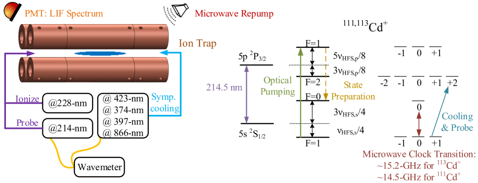
Figure 1: Schematic of the experiment setup for the ^111,113Cd⁺ HFS measurements. Sympathetic cooling technology is used to maintain the Cd⁺ cloud at low temperatures and improve measurement accuracy. The energy level scheme (not to scale) for ^111,113Cd⁺ is also presented.

In obtaining the measured LIF spectrum (Fig. 2), the beam intensity is maintained below 5 $\mu$W/mm² (saturation parameter 0.0006) to reduce the cooling and heating effects of the probe beam. The fitted curve is the Voigt profile Zuo et al. (2019); Han et al. (2021), expressed as

$$F = F_{0}+(F_{L}\ast F_{G})(\nu),$$

$$F_{L}(\nu) = \frac{2A}{\pi}\frac{\nu_{L}}{4(\nu-\nu_{c})^{2}+\nu_{L}^{2}},$$

$$F_{G}(\nu) = \sqrt{\frac{4\ln 2}{\pi}}\frac{e^{-\frac{4\ln 2}{\nu^{2}_{G}}\nu^{2}}}{\nu_{G}},$$ (1)

where $F_{0}$ is the offset, $\nu$ is the laser beam frequency, $\nu_{c}$ is the ion resonance frequency, $A$ is the area, $\nu_{L}$ is the Lorentzian width, $\nu_{G}$ is the Gaussian width of Doppler broadening. The line profile is slightly asymmetrically because of the heating and cooling effects of the probe beam, which lead to a slight increase in the uncertainty of the estimated transition frequency.

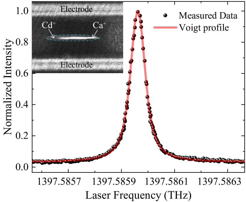
Figure 2: Typical LIF spectrum of Cd⁺, using ¹¹³Cd⁺ as an example. The frequency of the probe laser beam (214 nm wavelength) is scanned around the resonance frequency over a range of 600 MHz. The measured line profiles are fitted with a Voigt function. The inset is an image of the two-species ion cloud of Cd⁺ and Ca⁺ captured by an EMCCD camera; aberration has blurred the image.

Measurements present three sources of uncertainty:

• Statistical uncertainties. For the Cd⁺ $5s~{}^{2}S_{1/2}$–$5p~{}^{2}P_{3/2}$ transition, $\nu_{L}$ is 60.13 MHz which represent the natural width, the fitted $\nu_{G}$ is approximately 30 MHz, and the ion temperature is estimated to be approximately 100 mK. The statistical uncertainty associated with the transition frequencies of ¹¹⁴Cd⁺ and the ^111,113Cd⁺ is approximately 1 MHz, and thus the statistical uncertainty in their differences is approximately 1.4 MHz;

• Instrument uncertainties. The uncertainty arising from the drift in the wavemeter is less than 0.5 MHz in a laboratory environment Liu et al. (2018);

• Systematic uncertainties. Most systematic shifts are common to the $5s~{}^{2}S_{1/2}$–$5p~{}^{2}P_{3/2}$ transitions of both ¹¹⁴Cd⁺ and ^111/113Cd⁺ and thus cancel each other out. Because the $5s~{}^{2}S_{1/2}~{}(F=1)$–$5p~{}^{2}P_{3/2}~{}(F=2)$ transition of Cd⁺ is sensitive to magnetic fields, the Zeeman shift becomes the dominant contributor to systematic uncertainties.

In a weak field ($\mu_{B}B\sim 0.14$ MHz $\ll$ hyperfine constant $A$), the Zeeman shift for a specific energy level is expressed as

$$E_{Zeeman}=g_{F}M_{F}\mu_{B}\cdot B,$$ (2)

where $g_{F}$ is given by

$$g_{F}=\frac{F(F+1)+J(J+1)-I(I+1)}{2F(F+1)}g_{J},$$ (3)

where $J=L+S$ the total electron angular momentum ($S$ and $L$ the spin and orbital angular momenta), and $F=I+J$ the total angular momentum with $I$ denoting the nuclear spin. In typical conditions of our experiment, $B\sim 8000$ nT Miao et al. (2015, 2021). By introducing values $g_{J}=2.002257$ and $1.334056$ for the levels $5s~{}^{2}S_{1/2}$ and $5p~{}^{2}P_{3/2}$ calculated in this work (see text below), the Zeeman shift for the $5s~{}^{2}S_{1/2}~{}(F=1)$–$5p~{}^{2}P_{3/2}~{}(F=2)$ transition of Cd⁺ is estimated to be 0.11 MHz. Therefore, the total systematic shifts for the $5s~{}^{2}S_{1/2}~{}(F=1)$–$5p~{}^{2}P_{3/2}~{}(F=2)$ transitions of Cd⁺ are estimated to be below 0.5 MHz.

The final frequencies for the $5s~{}^{2}S_{1/2}~{}(F=1)$–$5p~{}^{2}P_{3/2}~{}(F=2)$ transitions of ^111,113Cd⁺ and that for $5s~{}^{2}S_{1/2}$–$5p~{}^{2}P_{3/2}$ of ¹¹⁴Cd⁺ are determined to be 4649.0(1.6) MHz and 4041.8(1.6) MHz, respectively.

In LS-coupling, the energy shifts after the hyperfine interaction are expressed as Foot et al. (2005)

$$E_{HFS}=A\langle I\cdot J\rangle=\frac{A}{2}[F(F+1)-I(I+1)-J(J+1)].$$ (4)

Therefore, for ^111,113Cd⁺, we have

$$\nu_{s,F=1\rightarrow p,F=2}^{111/113}=\nu_{s\rightarrow p}^{111/113}+\frac{1}{4}\nu_{HFS,s}-\frac{3}{8}\nu_{HFS,p},$$ (5)

where $\nu_{s,F=1\rightarrow p,F=2}^{111/113}$ is the transition frequency of $5s~{}^{2}S_{1/2}~{}(F=1)$–$5p~{}^{2}P_{3/2}~{}(F=2)$ of ^111,113Cd⁺; $\nu_{s\rightarrow p}^{111/113}$ is the transition frequency of $5s~{}^{2}S_{1/2}$–$5p~{}^{2}P_{3/2}$; $\nu_{HFS,s}$ is the HFS of $5s~{}^{2}S_{1/2}$; and $\nu_{HFS,p}$ is the HFS of $5p~{}^{2}P_{3/2}$. In reference to ¹¹⁴Cd⁺, through a linear transformation, Eq. (5) may be expressed as

$$\Delta\nu_{s,F=1\rightarrow p,F=2}^{111/113,114} = \Delta\nu_{s\rightarrow p}^{111/113,114}+\frac{1}{4}\nu_{HFS,s}^{111/113}$$

$$- \frac{3}{8}\nu_{HFS,p}^{111/113},$$

where $\Delta\nu_{s,F=1\rightarrow p,F=2}^{111/113,114}=\nu_{s,F=1\rightarrow p,F=2}^{111/113}-\nu_{s\rightarrow p}^{114}$ and $\Delta\nu_{s\rightarrow p}^{111/113,114}=\nu_{s\rightarrow p}^{111/113}-\nu_{s\rightarrow p}^{114}$. With our measurements, $\Delta\nu_{s,F=1\rightarrow p,F=2}^{111/113,114}$ are respectively 4649.0(1.6) MHz and 4041.8(1.6) MHz, whereas $\Delta\nu_{s\rightarrow p}^{111/113,114}$ are 1314.3(22)[023] MHz and 555.2(23)[008] MHz Hammen et al. (2018). From our previous measurements obtained through double-resonance microwave laser spectroscopy, the $\nu_{HFS,s}^{111/113}$ were accurately measured to be 14530507349.9(1.1) Hz Zhang et al. (2012) and 15199862855.02799(27) Hz Miao et al. (2021), from which we derived $\nu_{HFS,p}^{111/113}$ to be 794.6(3.6) MHz and 835.5(2.9) MHz.

III Theory

III.1 Multiconfiguration Dirac–Hartree–Fock approach

The MCDHF method C. Froese Fischer et al. (2016), as implemented in the Grasp computer package Jönsson et al. (2013); C. Froese Fischer et al. (2019), is employed to obtain wave functions referred to as atomic state functions. Specifically, they are approximate eigenfunctions of the Dirac Hamiltonian describing a Coulombic system given by

$$H_{\rm DC}=\sum_{i=1}^{N}(c~{}\bm{\alpha_{i}}\cdot\bm{p_{i}}+(\beta_{i}-1)c^{2}+V_{i})+\sum_{i<j}^{N}\frac{1}{r_{ij}},$$ (7)

where $V_{i}$ denotes the monopole part of the electron–nucleus interaction for a finite nucleus and $r_{ij}$ the distance between electrons $i$ and $j$; $\bm{\alpha}_{i}$ and $\beta_{i}$ are the Dirac matrices for electron $i$.

Electron correlations are included by expanding $|\Gamma J\rangle$, an atomic state function, over a linear combination of configuration state functions (CSFs) $|\gamma J\rangle$,

$$|\Gamma J\rangle=\sum_{\gamma}c_{\gamma}|\gamma J\rangle,$$ (8)

where $\gamma$ represents the parity and all the coupling tree quantum numbers needed to define the CSF uniquely. The CSFs are four-component spin-angular coupled, antisymmetric products of Dirac orbitals of the form

$$\phi({\bf r})=\frac{1}{r}\left(\begin{array}[]{c}P_{n\kappa}(r)\chi_{\kappa m}(\theta,\phi)\\ iQ_{n\kappa}(r)\chi_{-\kappa m}(\theta,\phi)\end{array}\right).$$ (9)

The radial parts of the one-electron orbitals and the expansion coefficients $c_{\gamma}$ of the CSFs are obtained by the self-consistent relativistic field (RSCF) procedure. In the following calculations of the relativistic configuration interaction (RCI), the Dirac orbitals are kept fixed, and only the expansion coefficients of the CSFs are determined for selected eigenvalues and eigenvectors of the complete interaction matrix. This procedure includes the Breit interaction and the leading quantum electrodynamic (QED) effects (vacuum polarization and self-energy).

The restricted active-set method is used in obtaining the CSF expansions by allowing single and double (SD) substitutions from a selected set of reference configurations to an active set (AS) of given orbitals. The configuration space is increased step by step by increasing the number of layers, specifically, a set of virtual orbitals. These virtual orbitals are optimized in the RSCF procedure while all orbitals of the inner layers are fixed.

The interaction between the electrons and the electromagnetic multipole moments of the nucleus splits each fine structure level into multiple hyperfine levels. The interaction couples the nuclear spin $\bm{I}$ with the total electronic angular momentum $\bm{J}$ to obtain total angular momentum $\bm{F=I+J}$.

The hyperfine contribution to the Hamiltonian is represented by a multipole expansion

$$H_{\rm HFS}=\sum_{k\geq 1}\bf{T^{(k)}}\cdot\bf{M^{(k)}},$$ (10)

where $\bf{T^{(k)}}$ and $\bf{M^{(k)}}$ are spherical tensor operators of rank $k$ in the electronic and nuclear spaces, respectively Lindgren and Rosén (1975). The $k=1$ term represents the magnetic dipole interaction, and the $k=2$ term the electric quadrupole interaction. Higher-order terms are minor and can often be neglected.

For the scheme considered in this work (^111,113Cd⁺ with $I=1/2$), only the magnetic dipole interaction is non-zero. To first-order, the fine-structure level $\gamma J$ is then split according to

$$\langle\Gamma IJFM_{F}|\bm{T^{(1)}\cdot M^{(1)}}|\Gamma IJFM_{F}\rangle$$ (11)

$$= (-1)^{I+J+F}\left\{\begin{array}[]{ccc}I&J&F\\ J&I&1\end{array}\right\}\langle\Gamma J||T^{(1)}||\Gamma J\rangle\langle\Gamma I||M^{(1)}||\Gamma I\rangle,$$

where the coefficient in curly brackets in the 6j symbol of the rotation group. The reduced matrix elements of the nuclear tensor operators are related to the conventional nuclear magnetic dipole moment,

$$\langle\Gamma I||M^{(1)}||\Gamma I\rangle=\mu_{I}\sqrt{\frac{(2I+1)(I+1)}{I}}.$$ (12)

The hyperfine interaction energy contribution to a specified hyperfine level is then given by

$$\langle\Gamma IJFM_{F}|\bm{T^{(1)}\cdot M^{(1)}}|\Gamma IJFM_{F}\rangle=\frac{1}{2}A_{J}C,$$ (13)

where $A_{J}$ is the magnetic dipole hyperfine constants

$$A_{J}=\frac{\mu_{I}}{I}\frac{1}{\sqrt{J(J+1)}}\langle\gamma J||T^{(1)}||\gamma J\rangle,$$ (14)

and $C=F(F+1)-J(J+1)-I(I+1)$.

However, this method discards the off-diagonal hyperfine interaction. This is not sufficient for ${}^{2}P_{1/2,3/2}$ because the hyperfine interaction between the two $F=1$ hyperfine levels is non-negligible owing to their minor splitting. To account for the off-diagonal hyperfine effects, we consider the second-order hyperfine interaction between ${}^{2}P_{1/2,3/2}$. The contribution associated with sublevel labelled $\gamma IJFM_{F}$ may be expressed as

$$\frac{|\langle\gamma IJFM_{F}|H_{hfs}|\gamma^{\prime}IJ^{\prime}FM_{F}\rangle|^{2}}{E_{J}-E_{J^{\prime}}}.$$ (15)

In the relativistic theory, choosing the direction of the magnetic field as the $z$-direction of the interaction and neglecting all diamagnetic contributions, the interaction between the magnetic moment of the atom and an external field may be written as

$$H_{M}=(N_{0}^{(1)}+\Delta N_{0}^{1})B,$$ (16)

where the last term is the Schwinger QED correction Cheng and Childs (1985). To first order, the fine-structure splitting in the energy level is

$$\langle\Gamma JM_{J}|N_{0}^{(1)}+\Delta N_{0}^{1}|\Gamma JM_{J}\rangle B$$ (17)

$$= \frac{M_{J}}{\sqrt{J(J+1)}}\langle\Gamma J||\bm{N^{(1)}+\Delta N^{(1)}}||\Gamma J\rangle B.$$

Factoring out the dependence on the $M_{J}$ quantum number, the energies are expressed in terms of the Landé $g_{J}$ factor

$$g_{J}=2\frac{\langle\Gamma J||\bm{N^{(1)}+\Delta N^{(1)}}||\Gamma J\rangle}{\sqrt{J(J+1)}}.$$ (18)

The energy splittings are then given by

$$g_{J}M_{J}\frac{B}{2}.$$ (19)

Table 1: Calculated hyperfine splitting (HFS) (in MHz) and Landé $g_{J}$ factors for $4d^{10}5s\ ^{2}S_{1/2}$ of ^111,113Cd⁺ obtained through the MCDHF approach.

	MCDHF2+RCI			MCDHF3+RCI
	111HFS	113HFS	$g_{J}$	111HFS	113HFS	$g_{J}$
5	11841	12386	2.002243	12925	13521	2.002242
6	13421	14040	2.002245	14096	14746	2.002247
7	13671	14301	2.002254	14414	15079	2.002250
8	13879	14518	2.002260	14476	15143	2.002256
9	13884	14524	2.002262	14515	15184	2.002257
10	13925	14567	2.002263	14541	15211	2.002257
11	13919	14561	2.002263	14532	15202	2.002257
12	13921	14562	2.002262	14537	15207	2.002257
Final	13921(7)	14563(7)	2.002262(2)	14536(9)	15206(9)	2.002257(1)

III.2 Computation Strategy

Initially, the MCDHF calculation was performed using the extended optimal-level scheme for the states of the $4d^{10}5s$ and $4d^{10}5p$ configurations, and these occupied orbitals were determined simultaneously and maintained throughout subsequent calculations. Because the $4f$ subshell in both the $4d^{10}5s$ and $4d^{10}5p$ configurations is vacant, imaging the strong pair correlations between $4d^{2}$ and $4f^{2}$, and between $4d^{2}$ and $5d^{2}$ is easy. The strong core-core (CC) correlation of the $4d$ electrons and the single valence $5s/5p$ electron do not allow us to include only the valence correlation; hence, our MCDHF calculation starts from the CC_4d mode, in which the $5s/5p$ and $4d$ electrons can be SD-excited to the $n\leq 8,l\leq 6$ level (AS₈, where ‘8’ labels the maximum principal quantum number in the corresponding AS). To investigate the correlation effects of the inner core electrons, we performed a few RCI calculations using the MCDHF wavefunctions derived from the CC_4d calculation. This calculation method is labelled MCDHF1+RCI in this paper. From the plots of the $A_{J}$ and $g_{J}$ factors for the ${}^{2}S_{1/2}$ and ${}^{2}P_{1/2,3/2}$ levels of ¹¹³Cd⁺ from this calculation method (Fig. 3), we see that they are sensitive to the core correlations, and even the core–valence (CV) correlation of the $1s$ orbital. To describe the wavefunctions better, we performed a second calculation that includes the strong CV and CC correlations in the RSCF procedure rather than only including the CV/CC correlations in the RCI procedure.

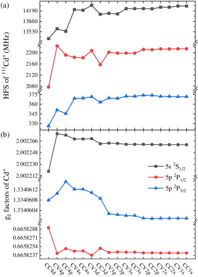
Figure 3: Hyperfine structure constants $A_{J}$ and Landé $g_{J}$ factors of the $4d^{10}5s\ ^{2}S_{1/2}$ and $4d^{10}5p\ ^{2}P_{1/2,3/2}$ levels for ¹¹³Cd⁺, from the various correlation models used in our MCDHF1+RCI calculation.

Table 2: Hyperfine splitting (HFS) (in MHz) and Landé $g_{J}$ factors for the $4d^{10}5p\ ^{2}P_{1/2,3/2}$ level of ^111,113Cd⁺. HFS_n.o indicate that no off-diagonal contributions were included, whereas HFS_w.o refers to HFS calculations with off-diagonal contributions.

	MCDHF2+RCI			MCDHF3+RCI
	111HFSn.o	113HFSn.o	$g_{J}$	111HFSn.o	113HFSn.o	111HFSw.o	113HFSw.o	$g_{J}$
$4d^{10}5p\ ^{2}P_{1/2}$
5	1816	1900	0.665833	2061	2156	2067	2150	0.665829
6	2099	2196	0.665825	2267	2371	2270	2368	0.665821
7	2054	2148	0.665825	2255	2359	2259	2355	0.665820
8	2142	2241	0.665820	2310	2416	2314	2413	0.665814
9	2123	2220	0.665822	2300	2406	2304	2403	0.665818
10	2146	2245	0.665821	2324	2432	2328	2428	0.665818
11	2144	2243	0.665820	2316	2422	2319	2419	0.665816
12	2145	2244	0.665820	2319	2425	2322	2422	0.665816
Final	2140(24)	2239(25)	0.665821(2)	2314(25)	2420(26)	2317(25)	2417(26)	0.665817(4)
$4d^{10}5p\ ^{2}P_{3/2}$
5	546	571	1.334062	644	674	650	680	1.334056
6	699	732	1.334057	787	824	791	827	1.334052
7	699	731	1.334060	768	803	772	807	1.334056
8	727	761	1.334060	794	830	797	834	1.334056
9	722	755	1.334062	786	822	789	826	1.334058
10	729	763	1.334060	789	828	793	832	1.334055
11	728	762	1.334059	789	824	792	828	1.334057
12	729	762	1.334060	789	825	793	829	1.334056
Final	727(8)	760(8)	1.334061(2)	789(8)	823(9)	792(8)	830(9)	1.334056(3)

In our second calculation, based on the above investigations, we included CV and CC correlations for the $4d$, $4p$, $4s$, $3d$, and $3p$ electrons, as well as the CV correlation down to the $1s$ subshell by allowing restricted SD excitations to $n\leq 12,l\leq 6$ (AS₁₂), in the RSCF calculation. RCI calculations were also performed to include the Breit and QED effects. Note that this calculation also started from the MCDHF calculation for the $4d^{10}5s$ and $4d^{10}5p$ configurations and hence is labelled MCDHF2+RCI.

In analyzing the wavefunction compositions from the MCDHF2+RCI calculation, we noticed strong correlations between $4d^{10}5s$, $4d^{8}4f^{2}5s$, and $4d^{9}4f5p$ configurations, and between $4d^{10}5p$, $4d^{8}4f^{2}5p$, and $4d^{8}5p5d^{2}$ configurations. Therefore, instead of starting from the DHF calculation where only $4d^{10}5s$ and $4d^{10}5p$ were included in the CSF list, we allowed the $4d$ and $5s/5p$ electrons to be SD-excited to {$5s,5p,5d,4f$} to generate the CSF list as a starting point of our third calculation approach. In this way, the spectroscopic orbitals together with the $5d$ and $4f$ orbitals are optimized together, and the correlation effect between the essential CSFs is included in the beginning. The CV and CC correlation effects are included by systematically increasing the virtual excitations to AS₁₂; this calculation method is labelled MCDHF3+RCI.

For $4d^{10}5s\ ^{2}S_{1/2}$, because there are no other levels with which to have strong hyperfine interactions, we only included the diagonal contributions to its HFS. The calculated HFSs and $g_{J}$ factors with an increasing AS size from MCDHF2+RCI and MCDHF3+RCI calculations are listed in Table 1. We find some fluctuations in our calculated HFSs with increasing AS size, but the values from the last few ASs generally tend to some specific value. We, therefore, took the average of the last three values (AS₁₀, AS₁₁, and AS₁₂) as our final calculated result, with the maximum difference between them taken as the calculation error. Although the final splitting for ¹¹³Cd⁺ from the MCDHF2+RCI calculation (i.e., 14563(7) MHz) is much smaller than the experimental measurement (i.e., 15199 MHz), the MCDHF3+RCI calculation, (15206(9) MHz) shows a significant improvement with the experimental value being within the estimated uncertainty of the latter calculation. Following a similar method, the $g_{J}$ factors of $2S_{1/2}$ from MCDHF2+RCI and MCDHF3+RCI calculations were 2.002262(2) and 2.002257(1), respectively. The HFSs and $g_{J}$ factors for $4d^{10}5s\ ^{2}P_{1/2,3/2}$ with an increasing AS are listed in Table 2. Following the same method as used in determining our final calculation results and their uncertainties, the HFSs for the ${}^{2}P_{3/2}$ level of ¹¹¹Cd⁺/¹¹³Cd⁺ from MCDHF2+RCI and MCDHF3+RCI calculations when not including the off-diagonal contributions are 727(8)/760(8) MHz and 789(8)/823(9) MHz, respectively. With off-diagonal contributions included, the MCDHF3+RCI results increase to 792(8)/830(9) MHz.

IV Results and discussions

The measured HFSs for the $5p~{}^{2}P_{3/2}$ level and the calculated HFSs and Landé $g_{J}$ factors for the $5s~{}^{2}S_{1/2}$ and $5p~{}^{2}P_{1/3,3/2}$ levels in this work are listed in Table 3; other experimental and calculated results are also listed for comparison. For the HFSs, our group’s previous high-accuracy measurements for the ^111,113Cd⁺ ground state provided an excellent benchmark for the atomic structure calculation of Cd⁺. The present HFSs for the $5s~{}^{2}S_{1/2}$ state calculated using the MCDHF method show stronger agreement with our previous experimental results than those of previous theoretical results Dixit et al. (2008); Li et al. (2018). The present measured HFSs for the $5p~{}^{2}P_{3/2}$ level is also in agreement with the present theoretical results. The cross-checking between experiment and theory ensures the reliability of the Cd⁺ $5p~{}^{2}P_{3/2}$ HFSs determined in this work. We recommend the adoption of 794.6(3.6) and 835.5(2.9) as the blue-shifted frequencies for optical pumping in the microwave-frequency standard based on ^111/113Cd⁺.

Regarding the Landé $g_{J}$ factors, there are no experimental results for Cd⁺. Accurate calculations of Landé $g_{J}$ factors has proven complicated even for alkali atoms and alkali-like ions because they are sensitive to electron correlations. Those calculated in this work using the MCDHF method show strong deviations from previous RCC results Han et al. (2019). The ground state Landé $g_{J}$ factor calculated in this work ($2.002257(1)$) agrees with the recent result calculated using the $\Lambda$-RCC theory ($2.002291(4)$) Yu et al. (2020b) to the fourth decimal place, although there is no overlap within their margins of uncertainty. To our knowledge, there also exists a significant difference in results between the $\Lambda$-RCC calculations with the configuration interaction and the many-body perturbation (CI+MBPT) calculations in Yb⁺ ground-state Landé $g_{J}$ factor Gossel et al. (2013); Yu et al. (2020b). Comparing the results of the same physical quantity from different calculation methods is also of great significance for developing atomic structure calculation models and understanding the role of electronic correlation effects. Therefore, we encourage more experimental and theoretical research on the Landé $g_{J}$ factors of Cd⁺.

For precaution, we recommend the value 2.00226(4) for the Cd⁺ ground state Landé $g_{J}$ factor in the evaluation of the SOZS of the microwave frequency standard of trapped Cd⁺ ions. The SOZS can be estimated using the Breit–Rabi formula,

$$\Delta\nu^{(2)}_{Zeem}(B)=-\frac{[g_{j}-g_{I}]^{2}\mu_{B}^{2}B^{2}}{2h^{2}A_{hf}},$$ (20)

for which $B\sim 8000$ nT for the Cd⁺ microwave frequency standard during actual operations. Thus, the fractional frequency shifts incurred when using the value of $g_{J}=2.00226(4)$ is $4.4\times 10^{-15}$. The fractional frequency shifts produced by this $g_{J}$ factor for the Cd⁺ ground-state can meet current accuracy requirements for the best Cd⁺ microwave frequency standard ($1.8\times 10^{-14}$). However, for further developments of this standard, the ground state $g_{J}$ factor of Cd⁺ also needs to be determined more accurately.

Table 3: Measured HFSs for $5p~{}^{2}P_{3/2}$ and the calculated HFSs and Landé $g_{J}$ factors of $5s~{}^{2}S_{1/2}$ and $5p~{}^{2}P_{1/3,3/2}$ of this work. Results of the Cd⁺ HFSs and Landé $g_{J}$ factors from other works are also listed for comparison.

111HFS	113HFS	$g_{J}$	Method
$5s~{}^{2}S_{1/2}$
14530.507	15199.863		Exp. Zhang et al. (2012)
14536(9)	15206(9)	2.002257(1)	MCDHF (This work)
14478(175)	15146(183)		RCC Li et al. (2018)
	15280		RCC Dixit et al. (2008)
		2.00286(53)	RCC Han et al. (2019)
		2.002291(4)	$\Lambda$-RCC Yu et al. (2020a)
$5p~{}^{2}P_{3/2}$
794.6(3.6)	835.5(2.9)		Exp. (This work)
	800		Exp. Tanaka et al. (1996)
792(8)	830(9)	1.334056(3)	MCDHF (This work)
794(12)	832(12)		RCC Li et al. (2018)
	812.04		RCC Dixit et al. (2008)
		1.33515(43)	RCC Han et al. (2019)
$5p~{}^{2}P_{1/2}$
2317(25)	2417(26)	0.665817(4)	MCDHF (This work)
2333(31)	2441(33)		RCC Li et al. (2018)
	2430		RCC Dixit et al. (2008)
		0.66747(83)	RCC Han et al. (2019)

V Conclusion

We reported on the determination of HFSs and Landé $g_{J}$ factors for the $5s~{}^{2}S_{1/2}$ and $5p~{}^{2}P_{1/2,3/2}$ levels of ^111,113Cd⁺. The HFSs of the $5p~{}^{2}P_{3/2}$ level was measured using the laser-induced-fluorescence technique. The Cd⁺ ions were co-trapped with Ca⁺ ions in the same linear ion trap and sympathetically cooled through the Coulomb interaction with laser-cooled Ca⁺ ions. Furthermore, the HFSs and Landé $g_{J}$ factors for both levels of interest were calculated using the MCDHF calculation. Three computational strategies were followed to account for the electronic correlation effects more comprehensively. The final calculated HFSs were in perfect agreement with the measured HFSs of this work and our previous work, which from cross-checks, demonstrated the reliability of the calculations and the experiments. The HFSs and Landé $g_{J}$ factors determined in this work can further improve the efficiency of the optical pumping procedure and the accuracy of the second-order Zeeman correction, and the stability and accuracy of the microwave frequency standard based on trapped Cd⁺ ions.

References

- Hinkley et al. (2013) N. Hinkley, J. A. Sherman, N. B. Phillips, M. Schioppo, N. D. Lemke, K. Beloy, M. Pizzocaro, C. W. Oates, and A. D. Ludlow, Science 341, 1215 (2013).
- Burt et al. (2021) E. Burt, J. Prestage, R. Tjoelker, D. Enzer, D. Kuang, D. Murphy, D. Robison, J. Seubert, R. Wang, and T. Ely, Nature 595, 43 (2021).
- Dzuba et al. (2016) V. Dzuba, V. Flambaum, M. Safronova, S. Porsev, T. Pruttivarasin, M. Hohensee, and H. Häffner, Nature Physics 12, 465 (2016).
- Wcisło et al. (2016) P. Wcisło, P. Morzyński, M. Bober, A. Cygan, D. Lisak, R. Ciuryło, and M. Zawada, Nature Astronomy 1, 1 (2016).
- Safronova et al. (2018) M. Safronova, D. Budker, D. DeMille, D. F. J. Kimball, A. Derevianko, and C. W. Clark, Reviews of Modern Physics 90, 025008 (2018).
- Bandi et al. (2011) T. Bandi, C. Affolderbach, C. E. Calosso, and G. Mileti, Electronics letters 47, 698 (2011).
- Prestage and Weaver (2007) J. D. Prestage and G. L. Weaver, Proceedings of the IEEE 95, 2235 (2007).
- Burt et al. (2016) E. A. Burt, L. Yi, B. Tucker, R. Hamell, and R. L. Tjoelker, IEEE transactions on ultrasonics, ferroelectrics, and frequency control 63, 1013 (2016).
- Diddams et al. (2004) S. A. Diddams, J. C. Bergquist, S. R. Jefferts, and C. W. Oates, Science 306, 1318 (2004).
- Schwindt et al. (2016) P. D. Schwindt, Y.-Y. Jau, H. Partner, A. Casias, A. R. Wagner, M. Moorman, R. P. Manginell, J. R. Kellogg, and J. D. Prestage, Review of Scientific Instruments 87, 053112 (2016).
- Mulholland et al. (2019a) S. Mulholland, H. Klein, G. Barwood, S. Donnellan, D. Gentle, G. Huang, G. Walsh, P. Baird, and P. Gill, Applied Physics B 125, 1 (2019a).
- Mulholland et al. (2019b) S. Mulholland, H. Klein, G. Barwood, S. Donnellan, P. Nisbet-Jones, G. Huang, G. Walsh, P. Baird, and P. Gill, Review of Scientific Instruments 90, 033105 (2019b).
- Hoang et al. (2021) T. M. Hoang, S. K. Chung, T. Le, J. D. Prestage, L. Yi, R. L. Tjoelker, S. Park, S.-J. Park, J. G. Eden, C. Holland, et al., Applied Physics Letters 119, 044001 (2021).
- Schmittberger and Scherer (2020) B. L. Schmittberger and D. R. Scherer, arXiv preprint arXiv:2004.09987 (2020).
- Miao et al. (2021) S. Miao, J. Zhang, H. Qin, N. Xin, J. Han, and L. Wang, arXiv preprint arXiv:2110.12353 (2021).
- Zhang et al. (2012) J. W. Zhang, Z. B. Wang, S. G. Wang, K. Miao, B. Wang, and L. J. Wang, Phys. Rev. A 86, 022523 (2012).
- Wang S. G (2013) M. K. W. Z. B. W. L. J. Wang S. G, Zhang J. W, Opt Express 21, 12434 (2013).
- Miao et al. (2015) K. Miao, J. W. Zhang, X. L. Sun, S. G. Wang, A. M. Zhang, K. Liang, and L. J. Wang, Opt. Lett. 40, 4249 (2015).
- Han et al. (2021) J. Han, H. Qin, N. Xin, Y. Yu, V. Dzuba, J. Zhang, and L. Wang, Applied Physics Letters 118, 101103 (2021).
- Li et al. (2018) C.-B. Li, Y.-M. Yu, and B. Sahoo, Physical Review A 97, 022512 (2018).
- Tanaka et al. (1996) U. Tanaka, H. Imajo, K. Hayasaka, R. Ohmukai, M. Watanabe, and S. Urabe, Physical Review A 53, 3982 (1996).
- Berkeland et al. (1998) D. Berkeland, J. Miller, J. C. Bergquist, W. M. Itano, and D. J. Wineland, Physical Review Letters 80, 2089 (1998).
- Phoonthong et al. (2014) P. Phoonthong, M. Mizuno, K. Kido, and N. Shiga, Applied Physics B 117, 673 (2014).
- Han et al. (2019) J. Han, Y. Yu, B. Sahoo, J. Zhang, and L. Wang, Physical Review A 100, 042508 (2019).
- Yu et al. (2020a) Y. Yu, B. Sahoo, and B. Suo, Physical Review A 102, 062824 (2020a).
- Zuo et al. (2019) Y. Zuo, J. Han, J. Zhang, and L. Wang, Applied Physics Letters 115, 061103 (2019).
- Liu et al. (2018) H. Liu, W. Yuan, F. Cheng, Z. Wang, Z. Xu, K. Deng, and Z. Lu, Journal of Physics B: Atomic, Molecular and Optical Physics 51, 225002 (2018).
- Foot et al. (2005) C. J. Foot et al., Atomic physics, Vol. 7 (Oxford University Press, 2005).
- Hammen et al. (2018) M. Hammen, W. Nörtershäuser, D. Balabanski, M. Bissell, K. Blaum, I. Budinčević, B. Cheal, K. Flanagan, N. Frömmgen, G. Georgiev, et al., Physical review letters 121, 102501 (2018).
- C. Froese Fischer et al. (2016) C. Froese Fischer, M. Godefroid, T. Brage, P. Jönsson, and G. Gaigalas, J. Phys. B: At. Mol. Opt. Phys. 49, 182004 (2016).
- Jönsson et al. (2013) P. Jönsson, G. Gaigalas, J. Bieroń, C. Froese Fischer, and I. Grant, Comput. Phys. Commun. 184, 2197 (2013).
- C. Froese Fischer et al. (2019) C. Froese Fischer, G. Gaigalas, P. Jönsson, and J. Bieroń, Comput. Phys. Commun. 237, 184 (2019).
- Lindgren and Rosén (1975) I. Lindgren and A. Rosén, in Case Studies in Atomic Physics, edited by E. McDANIEL and M. McDOWELL (Elsevier, 1975) pp. 93–196.
- Cheng and Childs (1985) K. T. Cheng and W. J. Childs, Phys. Rev. A 31, 2775 (1985).
- Dixit et al. (2008) G. Dixit, H. Nataraj, B. Sahoo, R. Chaudhuri, and S. Majumder, Physical Review A 77, 012718 (2008).
- Yu et al. (2020b) Y. M. Yu, B. K. Sahoo, and B. B. Suo, Phys. Rev. A 102, 062824 (2020b).
- Gossel et al. (2013) G. Gossel, V. Dzuba, and V. Flambaum, Physical Review A 88, 034501 (2013).