Abstract

We revisit the superradiant stability of Kerr-Newman black holes under a charged massive scalar perturbation. We obtain a newly suitable potential which is not singular at the outer horizon when a radial equation is expressed the Schrödinger-type equation in terms of the tortoise coordinate. From the potential analysis, we find a condition for the superradiant stability of Kerr-Newman black holes.

1 Introduction

For an asymptotically flat Kerr black hole, if the incoming scalar wave has a non-zero mass $\mu$, its mass would act as a natural mirror. In this case, one might find a superradiant instability of the black hole when the parameters of black holes and scalar field are in certain parameter spaces [1]. Here, a trapping well of the scalar potential plays the important role in making superradiant instability because superradiant modes are localized in the trapping well. If there is no trapping well, this black hole seems to be superradiantly stable.

Recently, the superradiant stability of Kerr-Newman (KN) black holes under a charged massive scalar perturbation can be achieved if two conditions of $qQ/\mu M>1$ and $r_{-}/r_{+}\leq 1/3$ are obtained from the potential analysis [2], in addition that the superradiance condition and the bound-state condition hold. Actually, the disappearance of a trapping well is a necessary condition for superradiant stability.

However, the potential determining the above two conditions seems to be inappropriate for analyzing the superradiant stability because $V(r\to r_{+})$ is singular and thus, it does not lead to $\omega^{2}-(\omega-\omega_{c})^{2}$ for imposing the superradiance condition. Furthermore, a defining equation for the potential (written by $r$) does not look like the Schrödinger-type equation since it was not written by making use of a tortoise coordinate $r_{*}$. The importance of $r_{*}$ arises from the fact that its range from $-\infty$ to $\infty$ exhausts the entire part of spacetime which is accessible to an observer outside the outer horizon [3]. If one uses $r$-coordinate, it covers a small region of $r\in[r_{+},\infty)$ only.

Importantly, we wish to point out that such a potential was originated from the derivation of a scalar equation expressed by $r$ [Eq.(15) in Ref. [4]] where a famous condition for a trapping well was derived as $\mu^{2}/2<\omega^{2}<\mu^{2}$ (or, $\mu/\sqrt{2}<\omega<\mu)$ in the study of Kerr black hole under a massive scalar perturbation. A potential derived in this way was used to determine the superradiant instability regime of the KN black hole  [5]. Also, a similar potential was employed subsequently in deriving the conditions for superradiant stability of Kerr black holes [6]. Very recently, a similar approach was applied to testing the extremal rotating black holes under a charged massive scalar perturbation [7], dyonic Reissner-Nordström (RN) black holes under a charged massive scalar perturbation [8], higher-dimensional non-extremal RN black holes under a massive scalar perturbation [9], and D-dimensional extremal RN black holes under a charged massive scalar perturbation [10]. It may not be valid to adopt such potentials to analyzing the superradiant (in)stability of a massive scalar propagating around rotating black holes.

In this work, we wish to revisit the superradiant stability of KN black holes under a charged massive scalar perturbation. We obtain an appropriate potential $V_{KN}(r\to r_{+})\sim\omega^{2}-(\omega-\omega_{c})^{2}$ when writing the Schrödinger-type equation in terms of the tortoise coordinate $r_{*}=\int[(r^{2}+a^{2})/\Delta]dr$. For $Q=0$, this reduces to the well-known potential for a massive scalar perturbation propagating around the Kerr black hole background [1]. From the analysis based on $V_{KN}(r)$, we could not derive the two conditions of $qQ/\mu M>1$ and $r_{-}/r_{+}\leq 1/3$ for the superradiant stability of a charged massive scalar propagating around the KN black holes. However, we obtain a condition for the superradiant stability.

2 A charged massive scalar on the KN black holes

First of all, we introduce the Boyer-Lindquist coordinates to represent the KN black hole with mass $M$, charge $Q$, and angular momentum $J$

$$ds^{2}_{\rm KN} = \bar{g}_{\mu\nu}dx^{\mu}dx^{\nu}$$ (1)

$$= -\frac{\Delta}{\rho^{2}}\Big{(}dt-a\sin^{2}\theta d\phi\Big{)}^{2}+\frac{\rho^{2}}{\Delta}dr^{2}+\rho^{2}d\theta^{2}+\frac{\sin^{2}\theta}{\rho^{2}}\Big{[}(r^{2}+a^{2})d\phi-adt\Big{]}^{2}$$

with

$$\Delta=r^{2}-2Mr+a^{2}+Q^{2},~{}\rho^{2}=r^{2}+a^{2}\cos^{2}\theta,~{}{\rm and}~{}a=\frac{J}{M}.$$ (2)

In addition, the electromagnetic potential is given by

$$\bar{A}_{\mu}=\frac{Qr}{\rho^{2}}\Big{(}-1,0,0,a\sin^{2}\theta\Big{)}.$$ (3)

The outer and inner horizons are determined by imposing $\Delta=(r-r_{+})(r-r_{-})=0$ as

$$r_{\pm}=M\pm\sqrt{M^{2}-a^{2}-Q^{2}}.$$ (4)

So, it is clear that $\Delta\to 0$, as $r\to r_{\pm}$.

A charged massive scalar perturbation $\Phi$ on the background of KN black holes is described by

$$(\bar{\nabla}^{\mu}-iq\bar{A}^{\mu})(\bar{\nabla}_{\mu}-iq\bar{A}_{\mu})\Phi-\mu^{2}\Phi=0.$$ (5)

Reminding the axis-symmetric background (1), it is convenient to separate the scalar perturbation into modes

$$\Phi(t,r,\theta,\phi)=\Sigma_{lm}e^{-i\omega t+im\phi}S_{lm}(\theta)R_{lm}(r)\,,$$ (6)

where $S_{\ell m}(\theta)$ is spheroidal harmonics with $-m\leq\ell\leq m$ and $R_{lm}(r)$ satisfies a radial part of the wave equation. Plugging (6) into (5), one has the angular equation for $S_{lm}(\theta)$ and the radial Teukolsky equation for $R_{lm}(r)$ as [11]

$$\frac{1}{\sin\theta}\partial_{\theta}\Big{(}\sin\theta\partial_{\theta}S_{\ell m}(\theta)\Big{)}+\left[\lambda_{lm}+a^{2}(\mu^{2}-\omega^{2})\sin^{2}{\theta}-\frac{m^{2}}{\sin^{2}{\theta}}\right]S_{lm}(\theta)=0,$$ (7)

$$\Delta\partial_{r}\Big{(}\Delta\partial_{r}R_{\ell m}(r)\Big{)}+U(r)R_{lm}(r)=0,$$ (8)

where

$$U(r)=[\omega(r^{2}+a^{2})-am-qQr]^{2}+\Delta[2am\omega-\mu^{2}(r^{2}+a^{2})-\lambda_{lm}].$$ (9)

Eq.(8) could be used directly for computing absorption cross-section and quasinormal modes of the scalar, and scalar clouds on the background of KN black holes.

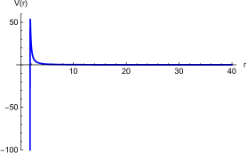
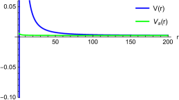
Figure 1: (Left) Potential $V(r)$ as function of $r$ with $M=1,Q=0.6,\omega=0.02,a=0.3,m=1,q=0.1,\lambda=12,\mu=0.05$ for $r\in[r_{+}=1.741,40]$. The potential is negatively singular ($-1.324\times 10^{13}$) at $r=r_{+}$. (Right) Potential $V(r)$ and its asymptotic potential $V_{a}(r)$ as functions of $r\in[r_{+},200]$. $V_{a}(r)$ mimics $V(r)$ for very large $r\geq 150$.

Introducing $\Psi_{lm}(r)=\sqrt{\Delta}R_{lm}(r)$, one finds easily that the radial equation (8) leads to

$$\frac{d^{2}\Psi_{lm}(r)}{dr^{2}}+\Big{[}\omega^{2}-V(r)\Big{]}\Psi_{lm}(r)=0,$$ (10)

where an effective potential $V(r)$ is given by [5, 2]

$$V(r)=\omega^{2} - \frac{1}{\Delta^{2}}\Big{[}\Big{(}\omega(r^{2}+a^{2})-am-qQr\Big{)}^{2}$$ (11)

$$+ \quad\quad\Delta\Big{(}2am\omega-\mu^{2}(r^{2}+a^{2})-\lambda_{lm}\Big{)}+M^{2}-a^{2}-Q^{2}\Big{]}.$$

We note that $V(r)$ was obtained just by imposing on the disappearance of $\Psi^{\prime}_{lm}$ in Eq.(10). Here, it is important to point out that Eq.(10) is not a proper Schrödinger-type (one-dimensional) equation expressed in terms of a tortoise coordinate $r_{*}$. As is shown in (Left) Fig. 1, $V(r)$ is not a suitable potential to analyze the superradiant stability because $V(r\to r_{+})$ is negatively singular like ‘$-1.324\times 10^{13}$’. This arises because $\Delta\to 0$ as $r\to r_{+}$ in the denominators. Instead, to find the superradiance condition, one should have $V(r\to r_{+})\sim\omega^{2}-(\omega-\omega_{c})^{2}$ where $\omega_{c}$ the critical frequency is given by

$$\omega_{c}=m\Omega_{H}+q\Phi_{H}$$ (12)

with $\Omega_{H}=a/(r_{+}^{2}+a^{2})$ and $\Phi_{H}=Qr_{+}/(r_{+}^{2}+a^{2})$.

To obtain a condition for superradiant instability (trapping well), it is necessary to introduce an asymptotic form $V_{a}(r)$. It was proposed that a trapping well exists if its first derivative must be positive ($V^{\prime}_{a}(r)>0$) [4]. On the other hand, a trapping well does not exist if its first derivative must be negative ($V^{\prime}_{a}(r)<0$) [2]. In this case, one finds $V_{a}(r)$ when expanding $V(r)$ for very large $r$ as

$$V(r\to\infty)\to V_{a}(r)+{\cal O}\Big{(}\frac{1}{r^{2}}\Big{)},$$ (13)

where

$$V_{a}(r)=\mu^{2}+\frac{2M\mu^{2}+2qQ\omega-4M\omega^{2}}{r}.$$ (14)

Here, its first derivative takes the form

$$V_{a}^{\prime}(r)=-\frac{2M\mu^{2}+2qQ\omega-4M\omega^{2}}{r^{2}}.$$ (15)

It was found that a condition for no trapping well leads to $(V_{a}^{\prime}(r)<0\to 2M\mu^{2}+2qQ\omega-4M\omega^{2}>0)$, which implies one condition of $qQ/\mu M>1$. However, from (Right) Fig. 1, $V_{a}(r)$ may represent $V(r)$ well for very large $r\geq 150$. So, the bound of $qQ/\mu M>1$ might not be regarded as a necessary condition for no trapping well. It suggests that the asymptotic potential $V_{a}(r)$ should include ${\cal O}(1/r^{2})$-terms to represent $V(r)$ for large $r\geq 20$ appropriately. The other condition of $r_{-}/r_{+}\leq 1/3$ was derived from the potential analysis under the condition of $qQ/(\mu M)>1$. However, this expression should be replaced by

$$\frac{r_{-}}{r_{+}}\leq\frac{1}{2\sqrt{\Big{(}\frac{a}{r_{+}}\Big{)}^{2}+1}-1}.$$ (16)

Up to now, we have briefly explained how two conditions for superradiant stability are derived from the analysis of potential $V(r)$ in (11). At this stage, we wish to mention that all analyses based on $V(r)$ may lead to the undesirable results.

3 Superradiance analysis with a new potential

Let us introduce the tortoise coordinate $r_{*}$ implemented by $dr_{*}=\frac{r^{2}+a^{2}}{\Delta}dr$ to derive the Schrödinger-type equation. In this case, our interesting region of $r\in[r_{+},\infty]$ could be mapped into the whole region of $r_{*}\in[-\infty,\infty]$, which implies that the inner region of $r<r_{+}$ is irrelevant to analyzing the superradiant stability. Then, the radial equation (8) takes a form of the Schrödinger-type equation when setting $\Psi_{lm}(r)=\sqrt{a^{2}+r^{2}}R_{lm}(r)$

$$\frac{d^{2}\Psi_{lm}(r_{*})}{dr_{*}^{2}}+\Big{[}\omega^{2}-V_{KN}(r)\Big{]}\Psi_{lm}(r_{*})=0,$$ (17)

where the well-defined potential $V_{KN}(r)$ is found to be [12]

$$V_{KN}(r)=\omega^{2} - \frac{3\Delta^{2}r^{2}}{(a^{2}+r^{2})^{4}}+\frac{\Delta[\Delta+2r(r-M)]}{(a^{2}+r^{2})^{3}}$$ (18)

$$+ \frac{\Delta\mu^{2}}{a^{2}+r^{2}}-\Big{[}\omega-\frac{am}{a^{2}+r^{2}}-\frac{qQr}{a^{2}+r^{2}}\Big{]}^{2}$$

$$- \frac{\Delta}{(a^{2}+r^{2})^{2}}\Big{[}2am\omega-\lambda_{lm}\Big{]}.$$

Here we observe that all $\Delta$ are located at the numerators, while all ‘$a^{2}+r^{2}$’ appear in the denominators, in compared to the location of $\Delta(a^{2}+r^{2})$ in denominators (numerators) for $V(r)$ in (11). This is because we use $R_{lm}(r)=\Psi_{lm}(r)/\sqrt{a^{2}+r^{2}}$ to derive $V_{KN}(r)$, whereas $R_{lm}(r)=\Psi_{lm}(r)/\sqrt{\Delta}$ is used to derive $V(r)$. In other words, we use the former to find out the Schrödinger-type equation (17) written by $r_{*}$, while the latter is necessary to make $\Psi^{\prime}_{lm}(r)$-term absent in Eq.(10) written by $r$. So, different choosing $R_{lm}(r)$ makes different overall scale factor in the potential.

Replacing $\lambda_{lm}$ by $\tilde{\lambda}_{lm}+a^{2}(\omega^{2}-\mu^{2})$, one finds that $\omega^{2}-V_{KN}(r)$ =$V_{\omega lm}(r)$ in Ref. [13]. It is noted that for $Q=0$, $V_{KN}(r)$ reduces to the potential $V_{K}(r)$ around the Kerr black hole [1] whose angular equation takes the form

$$\frac{1}{\sin\theta}\partial_{\theta}\Big{(}\sin\theta\partial_{\theta}S_{\ell m}(\theta)\Big{)}+\left[\tilde{\lambda}_{lm}+a^{2}(\omega^{2}-\mu^{2})\cos^{2}{\theta}-\frac{m^{2}}{\sin^{2}{\theta}}\right]S_{lm}(\theta)=0,$$ (19)

which implies a relation of $\lambda_{lm}=\tilde{\lambda}_{lm}+a^{2}(\omega^{2}-\mu^{2})(\lambda_{lm}<\tilde{\lambda}_{lm})$ with $\tilde{\lambda}_{lm}\sim l(l+1)+\cdots$. In this case, the last line of Eq.(18) is replaced by

$$-\frac{\Delta}{(a^{2}+r^{2})^{2}}\Big{[}2am\omega-a^{2}(\omega^{2}-\mu^{2})-\tilde{\lambda}_{lm}\Big{]}$$ (20)

which leads to potentials found in Refs. [1, 14, 15, 16] for studying the superradiant instability. In the non-rotating limit of $a\to 0$, we could recover the scalar potential from Eqs.(18) and (20) when studying superradiance in the RN black hole spacetimes under a charged massive scalar propagation [17, 18, 19, 20].

Before we proceed, let us explain a superradiant scattering by the KN black black holes. We find two limits such that $V_{KN}(r\to\infty)\to\mu^{2}$ and $V_{KN}(r\to r_{+})\to\omega^{2}-(\omega-\omega_{c})^{2}$. The latter limit is obviously achieved because $\Delta\to 0$ as $r\to r_{+}$. In this case, we have standard scattering forms of plane waves as [21]

$$\Psi_{lm} \sim {\cal I}e^{-i\sqrt{\omega^{2}-\mu^{2}}r_{*}}(\leftarrow)+{\cal R}e^{+i\sqrt{\omega^{2}-\mu^{2}}r_{*}}(\rightarrow),\quad r_{*}\to+\infty(r\to\infty),$$ (21)

$$\Psi_{lm} \sim {\cal T}e^{-i(\omega-\omega_{c})r_{*}}(\leftarrow),\quad r_{*}\to-\infty(r\to r_{+})$$ (22)

with the ${\cal T}({\cal R})$ the transmission (reflection) amplitudes. The Wrongskian $W(\Psi,\Psi^{*})$ of the complex conjugate solutions $\Psi$ and $\Psi^{*}$ satisfies

$$i\frac{d}{dr_{*}}W(\Psi,\Psi^{*})=0,$$ (23)

which implies that

$$|{\cal R}|^{2}=|{\cal I}|^{2}-\frac{\omega-\omega_{c}}{\sqrt{\omega^{2}-\mu^{2}}}|{\cal T}|^{2}.$$ (24)

This means that only waves with $\omega>\mu$ propagate to infinity and the superradiant scattering occurs ($\rightarrow,~{}|{\cal R}|^{2}>|{\cal I}|^{2}$) whenever $\omega<\omega_{c}$. Actually, the superradiance is associated to having a negative absorption cross section [13]. However, it turned out that the scalar absorption cross section is always positive for plane waves. For the KN black hole, the total absorption cross section becomes negative for co-rotating spherical waves at low frequencies. The superradiance can occur for massive scalar waves as long as the superradiance condition

$$\omega<\omega_{c}$$ (25)

is satisfied. Now, we wish to describe the superradiant instability briefly. The interaction between a rotating black hole and a massive scalar field will prevent low frequency modes with $\omega<\mu$ from escaping to spatial infinity. It is well known that if a massive scalar with mass $\mu$ is scattered off by a rotating black hole, then for $\omega<\mu$, the superradiance with $\omega<\omega_{c}$ might have unstable modes because the mass term works effectively as a reflecting mirror. In this case, a potential shape between ergo-region and mirror-region has a local maximum (potential barrier) as well as a local minimum (trapping well) away from the outer horizon which generates a secondary reflection of the wave that was reflected from the potential barrier [1, 15, 16]. The secondary reflected wave will be reflected again in the far region. Since each scattering off the barrier in the superradiant region increases the amplitude of the wave, the process of reflections will continue with the increased energy of waves, leading to an instability. This implies a quasi-bound state which is an approximate energy eigenstate localized in the scattering region. When an incident wave enters the scattering region with the right energy $E=\omega^{2}$, it spends a long time trapped in the quasi-bound state before eventually escaping back to infinity. The corresponding boundary conditions imply an exponentially decaying wave away from trapping well and a purely outgoing wave near the outer horizon:

$$\Psi \sim e^{-\sqrt{\mu^{2}-\omega^{2}}r}({\rm bound-state}),\quad r_{*}\to\infty(r\to\infty),$$ (26)

$$\Psi \sim e^{-i(\omega-\omega_{c})r_{*}}(\rightarrow:~{}{\rm superradiance}),\quad r_{*}\to-\infty(r\to r_{+}).$$ (27)

Considering a time-dependance $e^{-i\omega t}$ in (6), the outgoing wave could be achieved when satisfying $\omega<\omega_{c}$. To obtain a decaying mode at spatial infinity, one needs to have a bound-state condition of $\omega<\mu$. Therefore, the conditions for the superradiant instability are given by

$$\omega<\omega_{c},\quad\omega<\mu.$$ (28)

Importantly, the other (necessary) condition comes from the existence of a local minimum (a positive trapping well). The stable/unstable nature is selected by a shape of the potential. If there is no trapping well, it corresponds to a superradiant stability. As is shown in (Right) Fig. 2, $V_{KN}(r\to r_{+})\simeq\omega^{2}-(\omega-\omega_{c})$ is $-0.013$, while $V(r\to r_{+})=-1.324\times 10^{13}$ is singular [see (Left) Fig. 1]. The latter is inappropriate for imposing the superradiance condition (27) near the horizon. Here, we use the same parameters for obtaining $V_{KN}(r)$ and $V(r)$. Also, we find a significant difference between $V_{KN}(r\to r_{+})=0.06$ and $V(r\to r_{+})=-4.98\times 10^{31}$ in the Kerr black hole when setting $q=Q=0$ with the same parameters. Thus, it is conjectured that there is no parameter space for which $V(r)$ matches $V_{KN}(r)$ closely because their dependance of $\Delta$ is quite different.

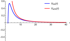
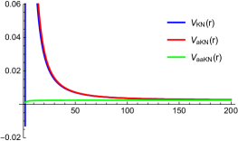
Figure 2: (Left) Potential without trapping well $V_{KN}(r)$ as function of $r\in[r_{+}=1.741,40]$ with $M=1,Q=0.6,\omega=0.02,a=0.3,m=1,q=0.1,\lambda_{lm}=12,\mu=0.05$. $V_{aKN}(r)$ mimics $V_{KN}(r)$ for $r\geq 20$. (Right) $V_{KN}(r_{+})$ is finite ($-0.013$) like as $\omega^{2}-(\omega-\omega_{c})^{2}=-0.012$. $V_{aaKN}(r)$ could imitate $V_{KN}(r)$ for $r\geq 150$. We check the condition of $\omega<\omega_{c}=0.13$ and $\omega<\mu$ in Eq. (28).

It seems that Fig. 2 corresponds to a superradiantly stable potential because we could not find a trapping well for $\omega<\omega_{c}=0.129$ and $\omega<\mu$. In this case, we observe that $\lim_{r\to 9225.94}V_{KN}(r)\to[\searrow\mu^{2}]$. Here, we find that a tiny well is located at $r=9225.94$ but it does not affect the superadiant stability.

To find out the existence of a local minimum, we consider $V_{aKN}(r)$ (when expanding $V_{KN}(r)$ for large $r$) given by

$$V_{KN}(r\to\infty)\to V_{aKN}(r)+{\cal O}\Big{(}\frac{1}{r^{3}}\Big{)},$$ (29)

where

$$V_{aKN}(r)=\mu^{2}-\frac{2(M\mu^{2}-qQ\omega)}{r}+\frac{\lambda_{lm}+Q^{2}(\mu^{2}-q^{2})}{r^{2}}.$$ (30)

Here, the third term plays an important role in making a trapping well because $\lambda_{lm}$ may take a large value. In this case, we point out that the condition for (no) trapping well is given by $(V^{\prime}_{aKN}(r)<0)~{}V^{\prime}_{aKN}(r)>0$. From (Right) Fig. 2, we know that $V_{aKN}(r)$ mimics $V_{KN}(r)$ well for large $r\geq 20$ and $V^{\prime}_{aKN}(r)<0$ implies no trapping well.

On the other and, $V_{aaKN}(r)$ defined through (when expanding $V_{KN}(r)$ for very large $r$)

$$V_{KN}(r\to\infty)\to V_{aaKN}(r)+{\cal O}\Big{(}\frac{1}{r^{2}}\Big{)},$$ (31)

where

$$V_{aaKN}(r)=\mu^{2}-\frac{2(M\mu^{2}-qQ\omega)}{r}$$ (32)

could represent $V_{KN}(r)$ for very large $r\geq 150$. This implies that $V_{aaKN}(r)$ is not sufficient to derive the condition for no trapping well. In this case, we stress that it is dangerous to derive a condition for no trapping well from $V_{aaKN}(r)$ only. If the condition of no trapping well is given by $V_{aaKN}^{\prime}(r)<0$, it implies a bound on $\omega$ as

$$\omega>\omega_{d}~{}{\rm with}~{}\quad\omega_{d}=\frac{M\mu^{2}}{qQ}.$$ (33)

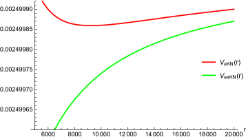
Figure 3: Asymptotic forms of $V_{aKN}(r)$ and $V_{aaKN}(r)$. $V_{aKN}(r)$ shows a tiny well located at $r=9228.69$ and it approaches $V_{aaKN}(r)$ for $r>9228.69$. All coefficients go together with Fig. 3.

However, we point out that this bound is not satisfied even for a superradiantly stable potential in Fig. 2 because of $\omega(=0.02)<\omega_{d}(=0.042)$. As is shown in Fig. 3, $V_{aKN}(r)$ has a tiny well at $r=9228.69$ and it approaches $V_{aaKN}(r)$ for $r>9228.69$. This explains why $\omega>\omega_{d}$ in Eq. (33) does not hold at asymptotic region.

At this stage, it is worth noting that $V_{aKN}(r)$ with $a=0$ and $\lambda_{lm}=l(l+1)$ and $V_{aaKN}(r)$ could be found exactly from the scalar potential obtained when charged massive scalar modes are impinging on the RN black holes [17, 18, 19, 20].

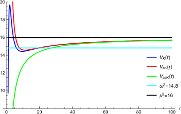
Figure 4: Positive Potential $V_{K}(r)=V^{Q=0}_{KN}(r)$ and its asymptotic potential $V_{aK}(r)=V^{Q=0}_{aKN}(r)$ around Kerr background as function of $r\in[r_{+}=1.063,100]$ with $M=1,Q=0,\omega=3.85,a=0.998,m=13,q=0,\lambda_{lm}=180,\mu=4$. The potential is finite (9.754) at $r=r_{+}$ and it has a trapping well (local minimum) at $r=9.6$. $V_{aK}(r)$ mimics $V_{K}(r)$ well for $r\geq 20$, while $V_{aaK}(r)$ mimics $V_{K}(r)$ for $r\geq 50$.

Now, we are in a position to introduce a potential with trapping well which is a necessary condition for the superradiant instability. Firstly, we consider a massive scalar propagation on the Kerr black hole background. In this case, we find a positive potential shown in Fig. 4, which involves a trapping well (local minimum) located at $r=9.6$ and indicates $V^{\prime}_{aK}(r)>0$ for large $r$. Plotting $V_{K}$ in terms of the tortoise coordinate $r_{*}$, $V_{K}$ is invariant in the depth but its near-horizon region is stretched from $-\infty$ (the horizon) to 0. In this case, one may recover Fig. 2 in Ref. [1] with the regions I (ergo-region: near-horizon), II (barrier-region), III (well-region), and IV (mirror-region: far-region) [Fig. 7 in Ref. [15] and Fig. 15 in Ref. [16]]. Three (II, III, IV) are essential for realizing superradiant instability and these regions are divided by imposing the turning point condition of $V_{K}=\omega^{2}$. Here, we note that there are quasi-bound states but there are no genuine bound states because the potential is purely repulsive ($V_{K}(r)>0$, everywhere).

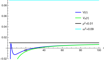
Figure 5: Potential $V(r)$ as function of $r$ with $M=1,Q=0.2,\omega=0.3,a=0.1,m=1,q=0.1,\lambda_{lm}=2,\mu=0.1$ for $r\in[r_{+}=1.975,100]$. The potential is negatively singular at $r=r_{+}$ with a negative well. $V_{a}(r)$ mimics $V(r)$ for $r\geq 40$ but $V(r)<\omega^{2}$ and $\omega>\mu$.

In case of $V(r)$ in Eq.(11), we display a case of potential with trapping well mentioned in Ref. [2] in Fig. 5. However, it is not suitable for representing an example for the superradiant instability because the bound-state condition ($\omega<\mu$) is not satisfied and there is no turning point (because of $V\ll\omega^{2}$). Furthermore, $V(r)$ is negatively singular ($-5.16\times 10^{6}$) at $r=r_{+}$ and it has a negative trapping well.

Considering a charged massive scalar on the KN black hole with $a=0.998$ (rapidly rotating black hole), we find a positive potential (see Fig. 6), which involves a trapping well (local minimum located at $r=9.61$) and shows $V^{\prime}_{aKN}(r)>0$ for large $r$. We note that $\lim_{r\to\infty}V_{KN}(r)\to[\nearrow\mu^{2}]$ for trapping well, compared to $\lim_{r\to 9225.94}V_{KN}(r)\to[\searrow\mu^{2}]$ for no trapping well in Fig. 2. This induces a quasi-bound state, leading to the superradiant instability. Comparing Fig. 6 with Fig. 2, it is worth noting that $V_{aKN}(r)$ includes a trapping well, but $V_{aaKN}(r)$ does not include a trapping well.

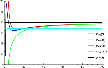
Figure 6: Positive potential $V_{KN}(r)$ and its asymptotic potential $V_{aKN}(r)$ as functions of $r\in[r_{+}=1.062,100]$ with $M=1,Q=0.01,\omega=3.85,a=0.998,m=13,q=0.2,\lambda_{lm}=180,\mu=4$. $V_{KN}(r)$ is finite (9.728) at $r=r_{+}$ and it has a trapping well located at $r=9.61$. Also, $V_{aKN}(r)$ imitates $V_{KN}(r)$ well for $r\geq 20$ whereas $V_{aaKN}(r)$ mimics $V_{KN}(r)$ for $r\geq 50$. We note $\omega<\omega_{c}=5.6398$ and $\omega<\mu$ as two conditions for superradiant instability.

This implies that it is not valid to derive a condition for no trapping well directly from $V_{aaKN}(r)$. In this case, we note that the condition for no trapping well [Eq.(33)] violates because of $\omega(=3.85)<\omega_{d}=8000$.

At this stage, we wish to mention the relation between tortoise coordinate and trapping well. We know from Eq. (18) that the first line without $\omega^{2}$ represents the effect of introducing the tortoise coordinate $r_{*}$, while the last two lines come from $-U(r)/(a^{2}+r^{2})^{2}$ in Eq. (9). Actually, the latter determines the asymptotic potential $V_{aKN}(r)$ in Eq. (30) completely whose third term plays an important role in making a trapping well for a large $\lambda_{lm}$. This means that $V^{\prime}_{aKN}(r)$ in assessing the trapping well is not affected by introducing the tortoise coordinate. Since $V^{\prime}_{aKN}(r)>0$ for large $r$ implies the presence of a trapping well, introducing the tortoise coordinate $r_{*}$ does not affect the presence of a trapping well. However, let us compare $V(r)$ in Fig. 5 with $V_{KN}(r)$ in Fig. 6. Even though they have a well, the former does not satisfy the bound-state condition ($\omega<\mu$), it is negatively singular at the horizon, and it has a negative trapping well.

To obtain stationary bound-state resonances, one has two conditions of $\omega=\omega_{c}$ and $\omega<\mu$. They correspond to marginally stable modes of the scalar field with Im[$\omega$]=0, leading to scalar clouds. In fact, such stationary resonances saturate the superradiance condition Eq.(25). However, even for weakly bound stationary resonances ($\omega=\omega_{c}\leq\mu$), there exist several distinct physical regimes [11]. We display a potential of stationary bound-state resonances in Fig. 7, which does not include a trapping well [12]. This potential is similar to Fig. 2 except $\omega=\omega_{c}$.

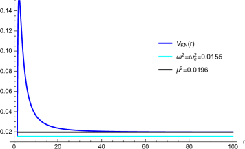
Figure 7: Stationary resonance potential $V_{KN}(r)$ as function of $r\in[r_{+}=1.4243,100]$ with $M=1,Q=0.9,\omega=0.1245,a=0.1,m=1,q=0.12,\lambda_{lm}=2,\mu=0.14$. $V_{KN}(r\to r_{+})$ is finite ($\omega^{2}=0.0155$). We note “$\omega=\omega_{c}$ and $\omega<\mu$” to meet the condition for stationary bound-state resonances.

Finally, we summarize four cases for a massive scalar propagating around the KN black holes:
(i) superradiant scattering $\to$ $\omega<\omega_{c}$ and $\omega>\mu$.
(ii) stationary bound-state resonances $\to$ $\omega=\omega_{c}$ and $\omega<\mu$.
(iii) superradiant instability $\to$ $\omega<\omega_{c}$ and $\omega<\mu$ with a positive trapping well.
(iv) superradiant stability $\to$ $\omega<\omega_{c}$ and $\omega<\mu$ without a positive trapping well.

4 Scalar waves in the far-region

It is important to know the scalar wave forms in the far-region to distinguish between trapping well and no trapping well. In this direction, we wish to derive wave functions in the far-region.

In the far-region where we have $r_{*}\sim r$ [$\Psi_{lm}(r)\sim rR_{lm}(r)$], we obtain an equation from Eqs. (17) and (30) as

$$\Big{[}\frac{d^{2}}{dr^{2}}+\omega^{2}-V_{aKN}(r)\Big{]}\Psi_{lm}=0$$ (34)

whose solution is given by the confluent Hypergeometric function $U[a,b,x]$ as

$$\Psi_{lm} = c_{1}e^{-\sqrt{\mu^{2}-\omega^{2}}r}\Big{(}2\sqrt{\mu^{2}-\omega^{2}}r\Big{)}^{\frac{1}{2}+\tilde{m}}$$ (35)

$$\times U\Big{[}\frac{1+2\tilde{m}}{2}-\frac{M\mu^{2}-qQ\omega}{\sqrt{\mu^{2}-\omega^{2}}},1+2\tilde{m},2\sqrt{\mu^{2}-\omega^{2}}r\Big{]}.$$

with

$$\tilde{m}=\frac{1}{2}\sqrt{1+4[\lambda_{lm}+Q^{2}(\mu^{2}-q^{2})]}.$$ (36)

Here we find an asymptotic bound-state of $e^{-\sqrt{\mu^{2}-\omega^{2}}r}$ appeared in (26).

If one uses $V_{aaKN}(r)$ in Eq.(32) with $\tilde{m}=1/2$, its solution is given by

$$\Psi_{lm}=c_{2}e^{-\sqrt{\mu^{2}-\omega^{2}}r}\Big{(}2\sqrt{\mu^{2}-\omega^{2}}r\Big{)}~{}U\Big{[}1-\frac{M\mu^{2}-qQ\omega}{\sqrt{\mu^{2}-\omega^{2}}},2,2\sqrt{\mu^{2}-\omega^{2}}r\Big{]}.$$ (37)

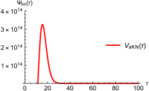
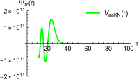
Figure 8: Radial modes $\Psi_{lm}$ as function of $r\in[11.3,100]$ with trapping well: (Left) quasi-bound state with $V_{aKN}(r)$ and (Right) oscillation with $V_{aaKN}(r)$. All parameters go together with Fig. 6.

Let us observe radial modes $\Psi_{lm}(r)$ for the case of superradiant instability (see Fig. 6). As is shown in (Left) Fig. 8, Eq.(35) shows a quasi-bound state followed by exponentially decaying mode, whereas Eq.(37) indicates an oscillation followed by exponentially decaying mode [see (Right) Fig. 8].

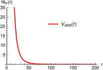
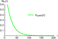
Figure 9: Radial modes $\Psi_{lm}$ as function of $r\in[12,100]$ without trapping well: (Left) exponentially decaying function with $V_{aKN}(r)$ and (Right) exponentially decaying function with $V_{aaKN}(r)$. All parameters go together with Fig. 2.

Contrastively, we consider radial modes for the potential without trapping well (shown in Fig. 2), implying superradiant stability. As is shown in Fig. 9, Eqs.(35) and (37) show exponentially decaying modes, describing bound states.

From (Left) Fig. 8 and (Left) Fig. 9, we observe a difference between quasi-bound state and bound state. It depends on the sign of the first argument $a$ in the confluent hypergeometric function $U[a,b,x]$ in Eq.(35). As is shown in (Left) Fig. 10, the superradiant instability (trapping well) could be achieved whenever $a$ is negative as

$$a<0\to\quad\frac{M\mu^{2}-qQ\omega}{\sqrt{\mu^{2}-\omega^{2}}}>\tilde{m}+\frac{1}{2}$$ (38)

together with $\omega<\omega_{c}$ and $\omega<\mu$. On the other hand, from (Right) Fig. 10 we have the superradiant stability (no trapping well) for positive $a$ as

$$a>0\to\quad\frac{M\mu^{2}-qQ\omega}{\sqrt{\mu^{2}-\omega^{2}}}<\tilde{m}+\frac{1}{2}$$ (39)

together with $\omega<\omega_{c}$ and $\omega<\mu$.

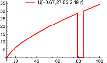
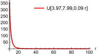
Figure 10: (Left) Confluent hypergeometric function $U[-0.8,27.8;2.17r]$ for quasibound state is an increasing function of $r$. (Right) Confluent hypergeometric function $U[3.97,7.99;0.09r]$ for bound state is a decreasing function of $r$.

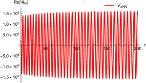
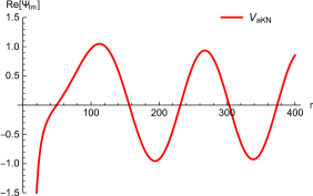
Figure 11: (Left) Real part of $\Psi_{lm}(r)$ as function of $r\in[10,200]$ where all parameters go together with Fig. 7 except $\omega=4>\mu=3.85$. (Right) Real part of $\Psi_{lm}(r)$ as function of $r\in[10,400]$ where all parameters go together with Fig. 3 except $\omega=0.05>\mu=0.02$.

On the other hand, it is interesting to observe superradiant scattering pictures for $\omega>\mu$. As is shown in Fig. 11, they are plane waves but their differences appear in the wave number and amplitude when adopting $V_{aKN}(r)$. These pictures are compared to (Left) Fig. 8 and (Left) Fig. 9. However, it is known that the scalar absorption cross section is always positive for plane waves. For the KN black hole, the total absorption cross section becomes negative for co-rotating spherical waves at low frequencies [13].

5 Discussions

It was reported that the superradiant stability of the KN black hole can be achieved if $qQ/\mu M>1$ and $r_{-}/r_{+}\leq 1/3$ are satisfied when analyzing the potential $V(r)$ in Eq.(11) [2]. Honestly, one could not regard $V(r)$ as a correct potential because it is negatively singular at the outer horizon as well as it was derived from a radial wave equation (8) without introducing the tortoise coordinate $r_{*}$. We note that the potential $V(r)$ was obtained just by imposing on the disappearance of $\Psi^{\prime}_{lm}$ in Eq.(10) from $\Psi_{lm}(r)=\sqrt{\Delta}R_{lm}(r)$ with $r$. It is worth noting that an opposite bound of $qQ/\mu M<1$ was firstly denoted as a condition for getting a trapping well (superradiant instability) around the KN black hole [22]. However, this condition is not satisfied simultaneously when imposing the superradiance condition ($\omega<\omega_{c}$) and thus, it is considered as a condition for bound states [18]. Also, we note that their effective potential $V_{\rm eff}(r)$ belongs to a shortened form because $\Psi_{\ell m}(r)=rR_{\ell m}(r)$ and a modified tortoise coordinate $x$ with $dx=r^{2}dr/\Delta$ are used to derive it.

In this work, we have found a correct potential $V_{KN}(r)$ in Eq.(18) from $\Psi_{lm}(r)=\sqrt{a^{2}+r^{2}}R_{lm}(r)$ with $r_{*}$ to discuss the condition for superradiant stability (no trapping well). To show the existence of a trapping well is a necessary condition for the superradiant instability because superradiant modes are localized in the trapping well [15]. If there is no trapping well, it means the superradiant stability. For superradiant stability, one needs to check the condition for no trapping well, in addition to two boundary conditions: $\omega<\omega_{c}$ and ($\omega<\mu$). Actually, the condition for no trapping well is given by $V^{\prime}_{aKN}(r)<0$. However, it is not easy to derive any analytic condition for no trapping well from $V^{\prime}_{aKN}(r)<0$ directly. As is shown in Fig. 8 (superradiant instability), Eq.(35) with $V_{aKN}(r)$ shows a quasi-bound state followed by exponentially decaying mode, whereas Eq.(37) with $V_{aaKN}(r)$ indicates an oscillation followed by exponentially decaying mode. On the other hand, for the case of superradiant stability (Fig. 9), Eqs.(35) and (37) show exponentially decaying modes only. From the observation of its asymptotic scalar function $U[a,b,x]$ in Fig. 10 based on $V_{aKN}(r)$, we find Eq.(38) for a condition of superradiant instability and Eq.(39) as a condition of superradiant stability.

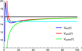
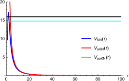
Figure 12: (Left) Potential $V_{KN}(r)$ and its asymptotic potentials $V_{aKN}(r)$ and $V_{aaKN}(r)$ as functions of $r\in[r_{+}=1.062,100]$ with $M=1,Q=0.01,\omega=3.85,a=0.998,m=13,q=0,\lambda_{lm}=180,\mu=4$. $V_{KN}(r\to r_{+})$ is 9.72 and a trapping well is located at $r=9.6$. We note $\omega<\omega_{c}=6.11$ and $\omega<\mu$ as the condition for superradiant instability. (Right) Potential $V_{KN}(r)$ and its asymptotic potentials $V_{aKN}(r)$ and $V_{aaKN}(r)$ as functions of $r\in[r_{+}=1.062,100]$ with $M=1,Q=0.01,\omega=3.85,a=0.998,m=13,q=0.2,\lambda_{lm}=180,\mu=0$. There is no trapping well because of $\mu=0$ and $\omega<\mu$ is not satisfied.

Finally, we wish to discuss the limitation on superradiance and superradiant instability. As was shown in [21], black hole superradiance is a radiation enhancement process that allows for energy extraction from the black holes at the classical level. This process is available from the static charged black hole, the rotating black hole, the charged rotating black hole, and the analogue black hole geometries. On the other hand, Press and Teukolsky [23] have suggested the ‘rotating black hole-mirror bomb’ idea: if the superradiance emerging from a perturbed black hole were reflected back onto the rotating black hole by a spherical mirror, an initially small perturbation could be made to grow without bound [24]. This superradiant instability is caused by either the mirror (artificial wall) or the cavity (AdS background). The reflection will occur naturally if a perturbed bosonic field has a rest mass $\mu$ [25]. The superradiant instability is surely possible to occur in the KN black hole (see Fig. 6 for its charged massive scalar potential with trapping well) and in the Kerr black hole (see Fig. 4 for its massive scalar potential with trapping well). We could have the superradiant instability for a massive scalar with $q=0$ around the KN black hole [see (Left) Fig. 12 with trapping well], whereas it is hard to have the superradiant instability for a charged scalar with $\mu=0$ because there is no mirror [see (Right) Fig. 12 without trapping well]. In addition, it is worth noting that the superradiant instability is not found from a charged massive scalar around the RN black holes. However, the superradiant instability of a charged massive scalar could be obtained if the RN black hole is enclosed in a cavity [17, 18]. This is called the charged black hole-mirror bomb, which is a spherically symmetric analogue of the rotating black hole-mirror bomb.

Acknowledgments

This work was supported by a grant from Inje University for the Research in 2021 (20210040).

References

- [1] T. J. M. Zouros and D. M. Eardley, Annals Phys. 118, 139-155 (1979) doi:10.1016/0003-4916(79)90237-9
- [2] J. H. Xu, Z. H. Zheng, M. J. Luo and J. H. Huang, Eur. Phys. J. C 81, no.5, 402 (2021) doi:10.1140/epjc/s10052-021-09180-y [arXiv:2012.13594 [gr-qc]].
- [3] S. Chandrasekar, The Mathematical Theory of Black holes, (Oxford Press, New York, 1983).
- [4] S. Hod, Phys. Lett. B 708, 320-323 (2012) doi:10.1016/j.physletb.2012.01.054 [arXiv:1205.1872 [gr-qc]].
- [5] Y. Huang and D. J. Liu, Phys. Rev. D 94, no.6, 064030 (2016) doi:10.1103/PhysRevD.94.064030 [arXiv:1606.08913 [gr-qc]].
- [6] J. H. Huang, W. X. Chen, Z. Y. Huang and Z. F. Mai, Phys. Lett. B 798, 135026 (2019) doi:10.1016/j.physletb.2019.135026 [arXiv:1907.09118 [gr-qc]].
- [7] J. M. Lin, M. J. Luo, Z. H. Zheng, L. Yin and J. H. Huang, Phys. Lett. B 819, 136392 (2021) doi:10.1016/j.physletb.2021.136392 [arXiv:2105.02161 [gr-qc]].
- [8] Y. F. Zou, J. H. Xu, Z. F. Mai and J. H. Huang, Eur. Phys. J. C 81, no.9, 855 (2021) doi:10.1140/epjc/s10052-021-09642-3 [arXiv:2105.14702 [gr-qc]].
- [9] J. H. Huang, R. D. Zhao and Y. F. Zou, Phys. Lett. B 823, 136724 (2021) doi:10.1016/j.physletb.2021.136724 [arXiv:2109.04035 [gr-qc]].
- [10] J. H. Huang, [arXiv:2201.00725 [gr-qc]].
- [11] S. Hod, Phys. Rev. D 90, no.2, 024051 (2014) doi:10.1103/PhysRevD.90.024051 [arXiv:1406.1179 [gr-qc]].
- [12] C. L. Benone, L. C. B. Crispino, C. Herdeiro and E. Radu, Phys. Rev. D 90, no.10, 104024 (2014) doi:10.1103/PhysRevD.90.104024 [arXiv:1409.1593 [gr-qc]].
- [13] C. L. Benone and L. C. B. Crispino, Phys. Rev. D 99, no. 4, 044009 (2019) doi:10.1103/PhysRevD.99.044009 [arXiv:1901.05592 [gr-qc]].
- [14] S. R. Dolan, Phys. Rev. D 76, 084001 (2007) doi:10.1103/PhysRevD.76.084001 [arXiv:0705.2880 [gr-qc]].
- [15] A. Arvanitaki and S. Dubovsky, Phys. Rev. D 83, 044026 (2011) doi:10.1103/PhysRevD.83.044026 [arXiv:1004.3558 [hep-th]].
- [16] R. A. Konoplya and A. Zhidenko, Rev. Mod. Phys. 83, 793-836 (2011) doi:10.1103/RevModPhys.83.793 [arXiv:1102.4014 [gr-qc]].
- [17] C. A. R. Herdeiro, J. C. Degollado and H. F. Rúnarsson, Phys. Rev. D 88, 063003 (2013) doi:10.1103/PhysRevD.88.063003 [arXiv:1305.5513 [gr-qc]].
- [18] J. C. Degollado and C. A. R. Herdeiro, Phys. Rev. D 89, no.6, 063005 (2014) doi:10.1103/PhysRevD.89.063005 [arXiv:1312.4579 [gr-qc]].
- [19] L. Di Menza and J. P. Nicolas, Class. Quant. Grav. 32, no.14, 145013 (2015) doi:10.1088/0264-9381/32/14/145013 [arXiv:1411.3988 [math-ph]].
- [20] C. L. Benone and L. C. B. Crispino, Phys. Rev. D 93, no.2, 024028 (2016) doi:10.1103/PhysRevD.93.024028 [arXiv:1511.02634 [gr-qc]].
- [21] R. Brito, V. Cardoso and P. Pani, Physics,” Lect. Notes Phys. 906, pp.1-237 (2015) doi:10.1007/978-3-319-19000-6 [arXiv:1501.06570 [gr-qc]].
- [22] H. Furuhashi and Y. Nambu, Prog. Theor. Phys. 112, 983-995 (2004) doi:10.1143/PTP.112.983 [arXiv:gr-qc/0402037 [gr-qc]].
- [23] W. H. Press and S. A. Teukolsky, Nature 238, 211-212 (1972) doi:10.1038/238211a0
- [24] V. Cardoso, O. J. C. Dias, J. P. S. Lemos and S. Yoshida, Phys. Rev. D 70, 044039 (2004) [erratum: Phys. Rev. D 70, 049903 (2004)] doi:10.1103/PhysRevD.70.049903 [arXiv:hep-th/0404096 [hep-th]].
- [25] T. Damour, N. Deruelle and R. Ruffini, Lett. Nuovo Cim. 15, 257-262 (1976) doi:10.1007/BF02725534