Antimodes and Graphical Anomaly Exploration via Adaptive Depth Quantile Functions

Abstract

This work proposes and investigates a novel method for anomaly detection and shows it to be competitive in a variety of Euclidean and non-Euclidean situations. It is based on an extension of the depth quantile functions (DQF) approach. The DQF approach encodes geometric information about a point cloud via functions of a single variable, whereas each observation in a data set is associated with a single such function. Plotting these functions provides a very beneficial visualization aspect. This technique can be applied to any data lying in a Hilbert space.

The proposed anomaly detection approach is motivated by the geometric insight of the presence of anomalies in data being tied to the existence of antimodes in the data generating distribution. Coupling this insight with novel theoretical understanding into the shape of the DQFs gives rise to the proposed adaptive DQF (aDQF) methodology. Applications to various data sets illustrate the DQF and aDQF’s strong anomaly detection performance, and the benefits of its visualization aspects.

Keywords— multi-scale, object data, outlier detection, visualization, high dimensional data

1 Introduction

Anomaly detection (alternatively: outlier detection, novelty detection, etc.) can be regarded as the identification of rare observations in a data set that differ significantly from the remaining bulk of the data. Detection of anomalies is an important task, as anomalies can be related to problematic behavior, or to novelties, potentially driving scientific innovation, etc. There is no standard definition of an outlier or anomalous observation, though the definition provided by Hawkins (1980) captures the essence used in the current work:

…an observation which deviates so much from other observations as to arouse suspicion it was generated by a different mechanism.

Anomalous observations can be defined in terms of either density or distance. For instance, Hyndman (1996) and others have defined outliers as those lying in low density regions, while others (e.g. Burridge and Taylor, 2006, and Wilkinson, 2017) define them as observations lying far from the bulk of the data.

Considering these different points of view on outliers or anomalies, one sees that rare (anomalous) events obviously correspond to low density. Furthermore, the idea of an alternative mechanism $Q$ generating these observations relates to mixture distributions in the sense of Huber’s (1964) $\epsilon-$contamination model, where the data is generated via $(1-\epsilon)P+\epsilon Q,$ $\epsilon>0$ small and $P$ representing the non-anomalous mechanism. Thus, under this model, the presence of anomalies corresponds with the existence of antimodes, assuming $P$ and $Q$ have modes in sufficiently separated locations. Certainly, deviating substantially from the bulk of the data means that the geometry, at least “locally” around the anomalous point or anomalous “micro-cluster”, differs from that of non-anomalous points. Additionally, at least on a heuristic level, one can expect to see an antimode of the density along the line connecting such an anomaly and a non-outlying observation, and since this antimode lies between areas of higher density, its centrality can be expected to be larger than tail regions with similar density.

We explore the depth quantile function (DQF) approach put forward in Chandler and Polonik (2021) in relation to the anomaly detection task. By exploiting the multiscale geometric information contained in the DQFs, we also provide an adaptation of the DQF, termed adaptive DQF (aDQF), that is tailored to the specific task of anomaly detection and is partly motivated by an implicitly assumed low-dimensional manifold structure for the non-anomalous points.

Due to the lack of a clear definition of what constitutes a true anomaly, a graphical summary of data can provide the practitioner with valuable information about unusual observations in their data that they might investigate further, just as a standard box plot does in one dimension. The DQF provides such a visualization of the data that is shown to be highly beneficial for the anomaly detection task. These visualizations are standard output of an associated R package.

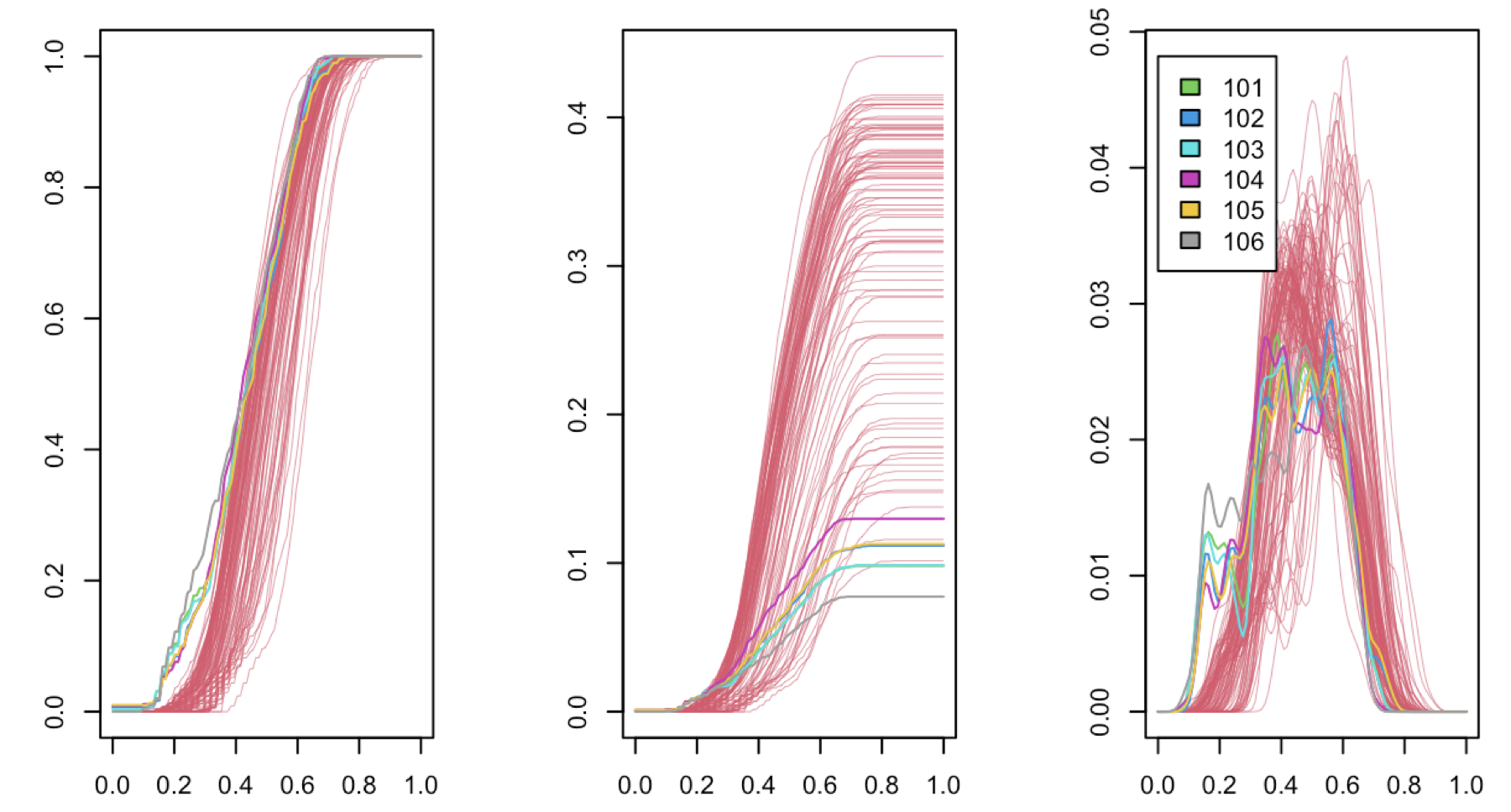
Figure 1: Functional representations via the DQF methodology for simulated data set; panels show standardized aDQFs, the aDQFs themselves, and their 1st derivatives, respectively; Data: $n=100$ observations, lying in a $d=30$ dimension annulus ($r=\frac{1}{3},R=1$) centered at origin drawn from a density decreasing as a function of the norm. Data $x_{101},\dots,x_{105}$ form an inlying micro-cluster inside the annulus, and $x_{106}=-x_{101}$ constitutes an isolated inlying anomaly. Anomalous observations (color-coded) show different behavior than non-anomalous observations, and micro-cluster separates itself from isolated anomaly.

It is important to note here that the visualization aspect of the DQF approach applies to any Hilbert space-valued data. In particular, the approach applies to data lying in a Euclidean space of arbitrary dimension and, in conjunction with the kernel trick, it also applies to non-Euclidean data. Indeed, as described below, the DQF maps Hilbert space valued data points to real valued functions of a single variable, which can then be easily plotted. Figure 1 shows three representations of such functions, described in detail below, for a constructed data set in a 30-dimensional Euclidean space that includes various notions of anomalies (an isolated point in the “hole” of the annulus that forms the support of the non-anomalous observations, and a micro-cluster of five points also in the “hole” but away from the first point).

The relation to antimodes becomes particularly evident when considering the DQF approach for $d=1$. Therefore we present this case which, in turn, establishes a perhaps unexpected connection to the concept of modal intervals put forward by Lientz (1974), and the related shorth plot (Sawitzki, 1994, Einmahl et al., 2010a,b).

The literature on tools for detecting anomalous observations is extensive, and it is impossible to provide a comprehensive overview. We refer to Hodge and Austin (2004), Aggarwal (2013) and Ruff et al. (2021) for surveys of both applications of this problem and various approaches to it.

Section 2 gives an introduction to the general DQF approach in both $d=1$ and higher, including discussion of tuning parameters, which yields the adaptive DQF. Section 3 considers anomaly detection in $d=1$ and elucidates the connections to existing tools, particularly the shorth. Anomaly detection for multivariate and object data, including numerical studies on both real and simulated data, is considered in Section 4. Section 5 presents a discussion of issues related to the implementation of this method including the accompanying R package. The final section contains technical proofs.

2 The DQF approach

Suppose we observe data lying in ${\mathbb{R}}^{d}.$ The DQF associated with an anchor point $x\in{\mathbb{R}}^{d}$ is a real-valued function of a one-dimensional parameter that is generated by considering random subsets of ${\mathbb{R}}^{d}$ containing $x$, and computing a measure of centrality of $x$ within each random subset. This then results in a distribution of centralities (for each anchor point $x$), and the quantile function of this distribution is the DQF corresponding to the anchor point (see below for details). The anchor point can be any point that can be covered by the random subsets considered. Below we consider two types of anchor points: data points, and midpoints between pairs of data points. The latter is not only motivated by our application, but also to alleviate challenges with notions of centrality in very high dimensions. The random subsets of ${\mathbb{R}}^{d}$ are randomly chosen spherical cones, and the measure of centrality used is based on Tukey’s (halfspace) depth (Tukey, 1975) applied to one-dimensional projections, where for a one-dimensional distribution function $F$, Tukey depth of $x\in{\mathbb{R}}$ is defined as $TD(x,F)=\min\{F(x),1-F(x)\}$.

The essence of choosing a random subset (spherical cone) and only considering points captured inside this cone is related to the concept of masking that Tukey introduced with PRIM-9 (see Fisherkeller et al. (1974), Friedman and Stuetzle (2002)). The idea of masking is to display low-dimensional projections of the subset of the data points not being masked, and to then interactively change the mask and inspect the resulting changes in the display. Rather than directly visualizing projections, the DQF approach first computes a summary statistic of the non-masked data points selected by the cone. This summary statistic is the centrality of the anchor point within the selected data. It then varies the mask randomly, and displays the quantile function of the summary statistic. This will be discussed further below.

2.1 The case ${\mathbf{d}\;}{\boldsymbol{=}\;}{\mathbf{1}}$

As said above, one of the advantages of the DQF approach is to provide a methodology for the visual exploration of geometric structure in data (including outliers, clusters, etc.) in any dimension, and even for non-Euclidean data via the kernel-trick. It turns out, however, that important insight can be gained by studying the DQF in dimension one, which also has the benefit of providing a gentle introduction to the DQF approach.

We first introduce the so-called depth functions. For $d=1$, the random subsets (cones) considered by the DQF approach are simply half-infinite intervals induced by a random split point $S$. For a probability measure $F$, we use the shorthand $F(x)=F((-\infty,x]),x\in{\mathbb{R}}$ to denote the distribution function. Given a point $x\in{\mathbb{R}}$, and a realization $s$ of $S$, define

$$d_{x}(s)=\begin{cases}\min\{F(x),F(s)-F(x)\}&\text{\rm if }\,x\leq s,\\ \min\{F(x)-F(s),1-F(x)\}&\text{\rm if }\,x>s,\end{cases}$$ (1)

where we notice, for instance when $s\geq x$, $d_{x}(s)$ is the Tukey depth of $x$ with respect to $F$ restricted to $(-\infty,s]$. Similarly, $d_{x}(s)$ also is the Tukey depth of $x$ in case $s<x,$ but this time for $F$ restricted to $[s,\infty).$ So, while the notion of centrality used by the DQF approach is Tukey’s (1975) data depth, it is with respect to an improper distribution, as we don’t rescale the mass on the subset.

Clearly, $d_{x}(s)$ is non-decreasing when $s$ moves away from $x$ in either direction, and the values for $s$ on the boundaries of the support of $F$ (which could be $\pm\infty$) are both equal to the global Tukey depth ${\rm TD}(x,F)$. Figure 2 shows functions $d_{x}(s)$ for a variety of $x$ values on a grid with $F$ admitting a symmetric density on $[0,1]$ comprised of two isosceles triangles.

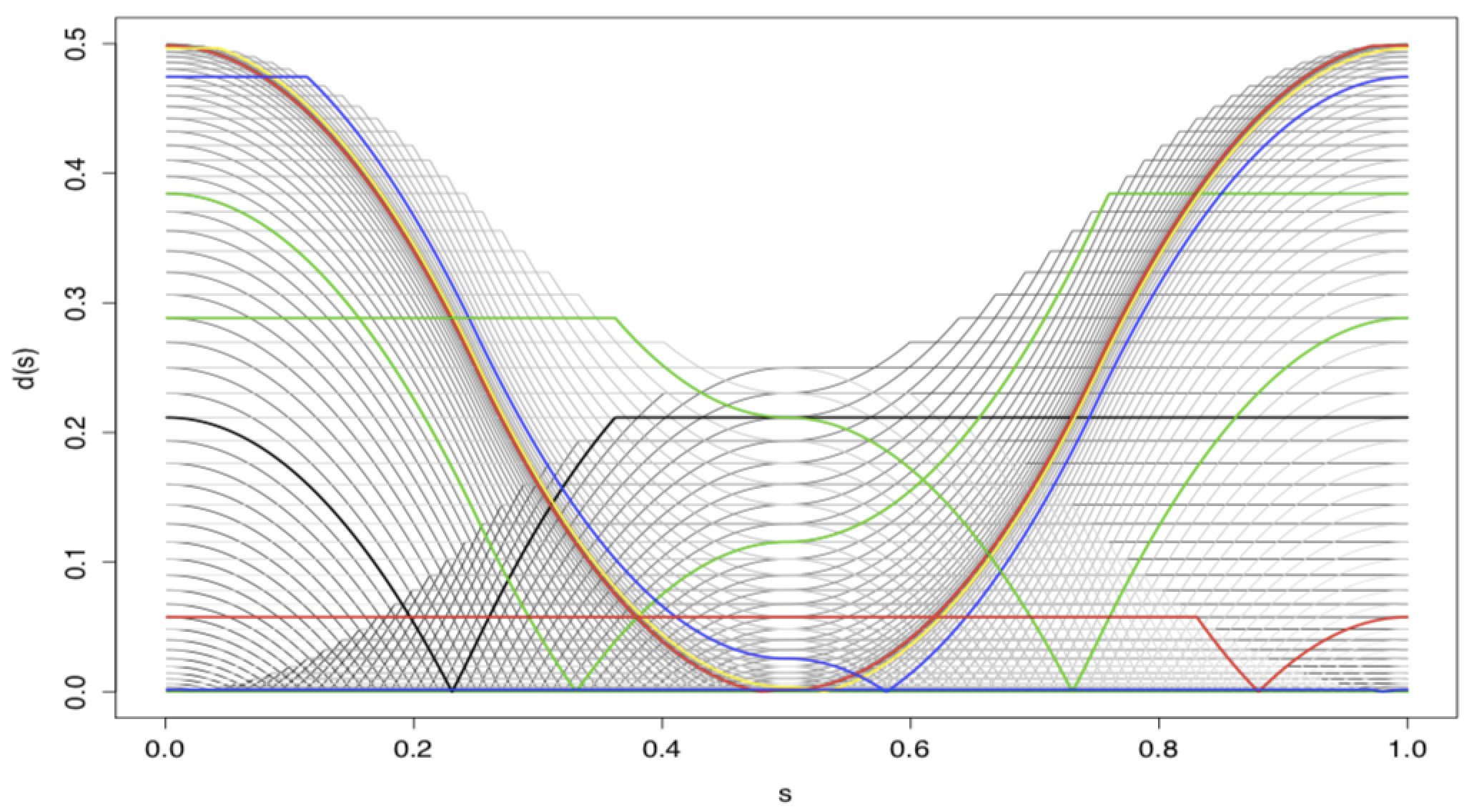
Figure 2: The function $d_{x}(s)$ for a grid of $x$ values, based on a symmetric density comprised of two isosceles triangle. The associated $x$ value for each curve is the point at which $d_{x}(s)=0$. Colored lines added to select points to aid visualization.

The random variable $S\sim G$ induces a distribution on $d_{x}(S)$, and the corresponding quantile function,

$$q_{x}(\delta)=\inf\{t\geq 0:G(d_{x}(S)\leq t)\geq\delta\},$$ (2)

is the object of interest, where, for a distribution $G$ and a measurable set $A$, we let $G(A)$ denote the probability content of $A$ under $G$. The parameter $\delta$ can be thought of as measuring the scale at which information is extracted.

Empirical versions are obtained by replacing $F$ with the empirical distribution $F_{n}$ based on the observations $X_{1},\ldots,X_{n},$ i.e. with

$$\widehat{d}_{x}(s)=\begin{cases}\min\{F_{n}(x),F_{n}(s)-F_{n}(x)\}&\text{\rm if }\,x\leq s,\\ \min\{F_{n}(x)-F_{n}(s),1-F_{n}(x)\}&\text{\rm if }\,x>s,\end{cases}$$ (3)

where we again use the shorthand $F_{n}(x)=F_{n}((-\infty,x]).$ Let

$$\widehat{q}_{x}(\delta)=\inf\{t\geq 0:G(\widehat{d}_{x}(S)\leq t)\geq\delta\}$$

(note that $G$ is the (marginal) distribution of $S$, so that $G(\widehat{d}_{x}(S)\leq t)$ depends on the data).

The following lemma addresses the median property and the zero interval property of the DQF. The median property is related to the concept of an antimode, while the presence of a zero interval is closely related to anomaly detection, as will be discussed further below. Figure 3 below illustrates the assertions of the lemma geometrically.

Lemma 2.1 (median property and zero interval).

Let $G$ be a continuous distribution with support $S_{g}\subseteq{\mathbb{R}}$ and density $g$ with $g(x)>0$ for $x\in S_{g}.$ Let $F$ be a continuous distribution with support $S_{f}\subseteq S_{g}$. For $x\in S_{g},$ let

$$\delta^{*}_{x}=\begin{cases}G\big{(}F^{-1}(2F(x))\big{)},&\text{for }\;F(x)\leq\frac{1}{2}\\ 1-G\big{(}F^{-1}(2F(x)-1)\big{)},&\text{for }\;F(x)\geq\frac{1}{2}.\end{cases}$$ (4)

Then, for $0\leq\delta<\delta^{*}_{x}$, there exists an interval $I_{x,\delta}=[a_{x,\delta},b_{x,\delta}]\subset[0,1]$ of $G$-measure $\delta$ with

$$q_{x}(\delta) =\frac{1}{2}F(I_{x,\delta})=F([a_{x,\delta},x])=F([x,b_{x,\delta}]).$$ (5)

Moreover,

$$q_{x}(\delta)=\begin{cases}0&\text{for }\;0\leq\delta\leq l_{x}\\ TD(x,F)&\text{for }\;\delta_{x}^{*}\leq\delta\leq 1\end{cases},$$ (6)

where $l_{x}=\sup\{G(b)-G(a):\,x\in[a,b],\,F([a,b])=0\}.$

The zero interval property expressed in (6) also holds in the multivariate case (see Lemma 2.2). It is quite important in the context of anomaly detection, as it provides an explanation for the empirical observation that the behavior of the DQF for small values of $\delta$ has a discriminatory effect in the context of anomaly detection. One of the situations in which this is of particular interest is when the anchor point $x$ is chosen as the midpoint between two observations, which might fall outside the support of $F$. All of this will be discussed in detail below.

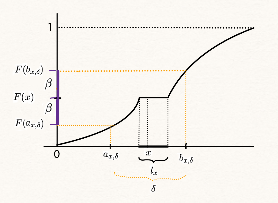
(a)

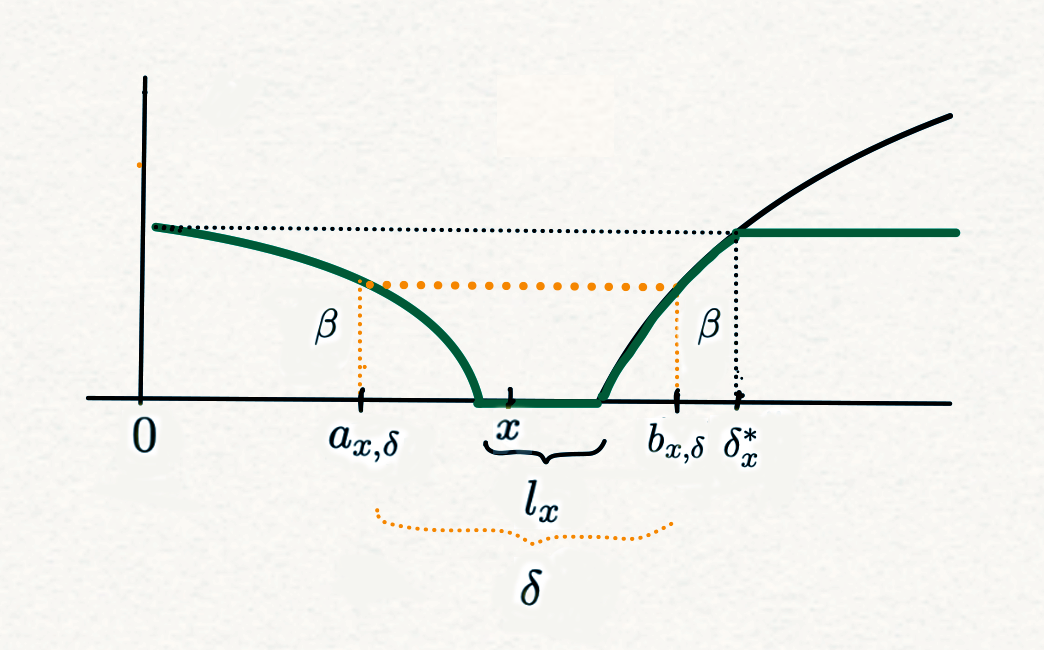
(b)

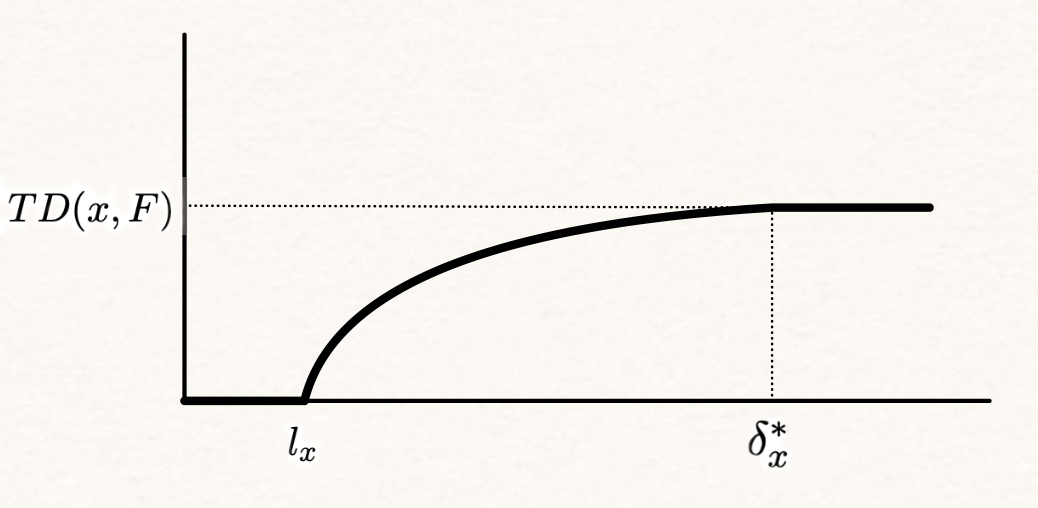
(c)

Figure 3: Illustration of Lemma 2.1 with $G=U[0,1]$: Panel (a) shows the cdf $F$ with a flat part around $x$, i.e. $x$ lies outside the support; here, the length of the flat part is $l_{x}$; for a given $\delta>0$, find an interval on the vertical axis symmetric about $F(x)$ (of length $2\beta$), such that its preimage is of length $\delta;$ this preimage is the interval $[a_{x,\delta},b_{x,\delta}]$; note that the $F$-measure of this interval by construction is $2\beta$, and having $F(x)$ in the center of the vertical interval corresponds to the median property; Panel (b) shows the corresponding depth function $d_{x}(s)$ (in green); it is obtained by reflecting the cdf to the left of $x$ upwards about the horizontal axis at height $F(x)$, then shifting the graph down by the amount $F(x)$ and capping the cdf (on the right) at height $F(x)$; the sublevel set of $d_{x}(s)$ at height $\beta$ now is the interval $[a_{x,\delta},b_{x,\delta}]$; note that there is no symmetric interval with nonnegative endpoints about $F(x)$ for $\beta>F(x)$, and this leads to the flat part on the right of $d_{x}(\delta);$ Panel (c) shows the DQF $q_{x}(\delta)$, which is $\beta$ as a function of $\delta.$

Corollary 2.1.

Consider the set-up of Lemma 2.1, and suppose that $F$ has density $F^{\prime}=f$. Then, for $x\in S_{g}$,

$$\lim_{\delta\to 0}\frac{2q_{x}(\delta)}{\delta} =\frac{f(x)}{g(x)}.$$

The statement directly follows from the representation of $q_{x}(\delta)$ given in (5) by assuming that $F$ is not constant in a neighborhood of $x$.

The above results, more precisely, (6) and Corollary 2.1, show that the DQF is informative at both large and small scales, i.e. for large and small values of $\delta$, motivating the usefulness of the entire function in examining a data set. An analogous property for the case $d\geq 2$ can be found in Chandler and Polonik (2021). This property is in contrast to other multi-scale methods, such as the mode tree (Minnotte and Scott, 1993), which transitions from $n$ modes to 1 (thus no information on either extreme), or a multi-scale version of the shorth which we discuss and explore in section 3.

2.2 The case ${\mathbf{d}\;}{\boldsymbol{>}\;}{\mathbf{1}}$

As localization is an important aspect of the DQF for small values of $\delta$, one finds that half-spaces as our random subsets will not suffice. Rather, we consider subsets of the data space formed by spherically symmetric cones with opening angle $\alpha$ strictly less than $\pi/4$ (the angle between a point on the surface of the cone and the axis of symmetry). We use spherical cones to not privilege any particular direction in our space beyond the specified axis of symmetry for the cone. The question is then how to put a distribution over cones in order to compute quantile functions.

First we discuss the construction of the empirical version of the DQF. For any two points in the data set, say $x_{i}$ and $x_{j}$, let $\ell_{ij}$ denote the line passing through them, and consider spherically symmetric cones $C_{ij}(s)$ with $\ell_{ij}$ as axis of symmetry, $s$ as the tip located on $\ell_{ij}$, and a fixed opening angle $\alpha$, which is a tuning parameter. Select a point $m_{ij}$ on that line as the “anchor point.” The choice of $m_{ij}$ might depend on the specific application considered. In our applications, we choose $m_{ij}=\frac{x_{i}+x_{j}}{2}$, the midpoint, but it could also be $x_{i}$, or $x_{j}$, as we are using in the one-dimensional case discussed above. See section 4.1 for discussion of this choice. The orientation of the cone $C_{ij}(s)$ is such that $m_{ij}$ is contained inside. In other words, the orientation of the cones flips depending on which side of $m_{ij}$ the tip lies.

Given any such cone $C_{ij}(s)$, split the cone into two parts $A_{ij}(s)$ and $B_{ij}(s)=C_{ij}(s)\setminus A_{ij}(s)$ with $A_{ij}(s)$ being the “top part” of the cone, obtained by cutting $C_{ij}(s)$ along a hyperplane orthogonal to $\ell_{ij}$ passing through $m_{ij}$. We sometimes also call these two type of sets $A$-sets (cones themselves) and $B$-sets (frustums). The base of $A_{x,y}(s)$ (or the top of $B_{x,y}(s)$) is considered to be part of $A_{x,y}(s)$ but not of $B_{x,y}(s)$. Then, the measure of centrality of $m_{ij}$ that we are using is the depth

$$\hat{d}_{ij}(s)=\min\big{(}F_{n}(A_{ij}(s)),F_{n}(B_{ij}(s))\big{)}.$$

Equivalently, one can think of constructing $\hat{d}_{ij}(s)$ by projecting the data lying inside the cone $C_{ij}(s)$ onto $\ell_{ij}.$ Then $\hat{d}_{ij}(s)$ is the one dimensional Tukey depth of $m_{ij}$ among these projections, again with respect to the improper empirical (sub)distribution.

Finally, we choose the tip randomly according to a distribution $G_{ij}(s)$ along the axis of symmetry $\ell_{ij}$. (Choosing $G_{ij}$ is discussed in 2.3.) The DQF $\hat{q}_{ij}(\delta)$ is then defined as the quantile function of the distribution of the random depths with respect to $G_{ij}(s)$, i.e.

$$\hat{q}_{ij}(\delta)=\inf\big{\{}t>0:\,G_{ij}(s:\hat{d}_{ij}(s)\leq t)\geq\delta\big{\}},$$

where, for a measurable set $D\subset\ell_{ij}$ we let $G(D)$ denote the $G$-measure of $D$. Note that $G_{ij}(s:\hat{d}_{ij}(s)\leq t)$ depends on all of the data. One might use different approaches to reduce the total number of functions $\hat{q}_{ij}(\delta)$ to consider. A natural approach is to use averaging: For each data point $x_{i},$ average the functions $\hat{q}_{ij}(\delta)$ over $j\neq i$, i.e. for each $x_{i}$, we consider

$$\overline{q}_{i}(\delta)=\frac{1}{n-1}\sum_{j=1\atop j\neq i}^{n}\hat{q}_{ij}(\delta).$$

More robust approaches include Winsorized averages, truncated averages, etc. A slightly different summary is to consider normalized averages of the DQFs of the form

$$\widetilde{q}_{i}(\delta)=\frac{\bar{q}_{i}(\delta)}{\bar{q}_{i}(1)}.$$

These normalized averages embed the global behavior of the DQF at all $\delta$ values and focus solely on the shape of the DQF.

Population versions of the empirical depth functions $\hat{d}_{ij}(s)$ and the corresponding empirical DQFs are defined as follows. For $x,y\in{\mathbb{R}}^{d}$, let $\ell_{x,y}$ denote the line passing through both $x$ and $y$. For $s\in\ell_{x,y}$ let $C_{x,y}(s)$ denote the spherically symmetric cone in ${\mathbb{R}}^{d}$ with tip $s$ containing the anchor point, say $m_{x,y}=\frac{x+y}{2},$ with axis of symmetry given by $\ell_{x,y}$, and with opening angle given by the tuning parameter $\alpha$. The hyperplane through $m_{x,y}$ perpendicular to $u$ again divides $C_{x,y}(s)$ into two sets, a cone $A_{x,y}(s)$ and a frustum $B_{x,y}(s),$ where for definiteness, the intersection of the hyperplane and the cone (the base of $A_{x,y}(s)$ or the top of $B_{x,y}(s)$) is considered to be part of $A_{x,y}(s)$ but not of $B_{x,y}(s)$. Then,

$$d_{x,y}(s)=\min\big{(}F(A_{x,y}),\,F(B_{x,y})\big{)}.$$

Similar to the empirical version, $d_{x,y}(s)$ is the one-dimensional Tukey depth of the (sub)distribution obtained by projecting the mass of the cone $C_{x,y}(s)$ onto the axis of symmetry $\ell_{x,y}$. Figure 4 illustrates this for a two-dimensional bi-modal density.

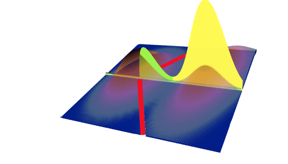
Figure 4: A 2-dimensional bimodal density (transparent blue to orange), a given anchor point $m_{x,y}$ (green/yellow region intersection), direction $\ell_{x,y}$ (green line in plane), and cone tip $s$ (convergence of red cone boundaries). Green/yellow function over $\ell_{x,y}$ indicates the probability mass inside the cone projected onto $\ell_{x,y}$. For this cone tip, $d_{x,y}(s)$ would equal the green area under the one-dimensional curve rather than the larger yellow area.

Again, choosing the tip randomly on the line $\ell_{x,y}$ according to $S\sim G=G_{x,y}$ results in a random variable $d_{x,y}(S)$ whose quantile function is the DQF $q_{x,y}(\delta)$. Formally,

$$q_{x,y}(\delta)=\inf\{t>0:\,G_{x,y}(d_{x,y}(S)\leq t)\geq\delta\}.$$

The empirical average $\overline{q}_{i}(\delta)$ corresponds to

$$\overline{q}_{x}(\delta)={\rm E}\big{[}q_{x,Y}(\delta)\big{]},\quad Y\sim F,$$

and similarly $\tilde{q}_{x}(\delta)=\frac{\overline{q}_{x}(\delta)}{\overline{q}_{x}(1)}$ is the normalized expected DQF. As already mentioned, a result for $d\geq 2$, analogous to Corollary 2.1 can be found in Chandler and Polonik (2021). The flatness of the DQF for anchor points lying outside the support of $F$, i.e. a result analogous to the last assertion of Lemma 2.1, also holds for $d\geq 2,$ as shown in Lemma 2.2.

We use the following setting: For a given distribution $F$ on ${\mathbb{R}}^{d}$ with compact support (for simplicity) and $x,y\in{\mathbb{R}}^{d}$, let $[a_{x,y},b_{x,y}]\subseteq\ell_{x,y}$ denote the range of the push-forward distribution on $\ell_{x,y}$ obtained by the projection map $\pi_{x,y}(z)$, which is the orthogonal projection of $z\in{\mathbb{R}}^{d}$ onto $\ell_{x,y}.$ We assume $\|b_{x,y}-a_{x,y}\|>0$. Let $G_{x,y}$ denote a continuous distribution on $[a_{x,y},b_{x,y}]$. This is a distribution on the “one-dimensional interval” of length $\|b_{x,y}-a_{x,y}\|$. Also, we represent $\ell_{x,y}$ as $\ell_{x,y}=\{z\in{\mathbb{R}}^{d}:\,z=m_{x,y}+tu_{x,y},t\in{\mathbb{R}}\}$, where $m_{x,y}$ is the anchor point, and $u_{x,y}\in S^{d-1}$ is the unit vector giving the direction of $\ell_{x,y}.$

Lemma 2.2 (zero interval property in multivariate settings).

Consider the above setting for given $x,y\in{\mathbb{R}}^{d}.$ Set

$$t^{\pm}_{x,y} =\inf_{t\geq 0}\{s=m_{x,y}\pm tu_{x,y},\;s\in[a_{x,y},b_{x,y}]\;\text{\rm and}\;F(A_{x,y}(s))\neq 0\}$$

and

$$s^{\pm}_{x,y} =m_{x,y}\pm t^{\pm}_{x,y}u.$$

Then,

$$q_{x,y}(\delta)=0\qquad\text{for }\;\;\delta\in[0,\delta_{x,y}],$$

where $\delta_{x,y}=G_{x,y}([s^{-}_{x,y},s^{+}_{x,y}]).$ In case $G_{x,y}=U[a_{x,y},b_{x,y}]$, the uniform distribution on $[a_{x,y},b_{x,y}],$ we can write $G_{x,y}([s^{-}_{x,y},s^{+}_{x,y}])=\frac{t^{+}_{x,y}+t^{-}_{x,y}}{\|b_{x,y}-a_{x,y}\|}.$ Furthermore, we have

$$\overline{q}_{x}(\delta)=0\qquad\text{for }\;\;\delta\in[0,\inf_{y}\delta_{x,y}].$$

Geometrically, the quantity $t^{+}_{x,y}+t^{-}_{x,y}=\|s^{+}_{x,y}-s^{-}_{x,y}\|$ is the sum of the heights of two cones $A_{x,y}(s^{+}_{x,y}),A_{x,y}(s^{-}_{x,y})$, see Figure 5. Note that the two cones point in opposite directions, and by definition of $t^{+}_{x,y}$ and $t^{-}_{x,y}$, they are chosen such that they give the largest spherically symmetric cones under consideration that do not intersect with the support of $F.$ Also note that the two cones belong to the same anchor point that is lying between the bases of these two cones.

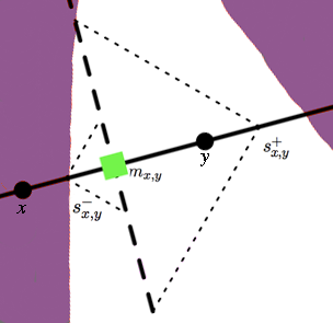
Figure 5: The point $y$ corresponds to an anomalous observation living outside the support (purple shaded region). This point is compared to the non-anomalous $x$, and the midpoint is used as the anchor point. The length of the zero-interval, $\delta_{x,y}$, is the $G-$measure of the interval $(s_{x,y}^{-},s_{x,y}^{+})$.

Suppose that the support of $F$ has a hole and the anchor point $m_{x,y}$ lies in this hole (think of $m_{x,y}$ as the midpoint between $x$ and $y$), then the $G_{x,y}$-measure of the combined heights, $\delta_{x,y}=G_{x,y}([s^{-}_{x,y},s^{+}_{x,y}]),$ measures some aspects of the geometry of the hole. Moreover, if, for a given $x$, there is a high probability that a randomly chosen $y$ is such that the corresponding anchor point lies off the support of $F$, then $\overline{q}_{x}(\delta)$ will also be small for a range of small values of $\delta.$ (Recall also that everything depends on the opening angle of the cones as well.)

Also note that Lemma 2.2 is a generalization of the one-dimensional case presented in the last part of Lemma 2.1. In this one-dimensional case there is of course no need to consider pairs since there is only one axis. For further discussion of the population version and theoretical properties of the corresponding estimators, see Chandler and Polonik (2021).

2.2.1 Discussion of the (near) zero-interval property

As indicated above, the behavior of the (average) DQF for small values of $\delta$ is quite useful for visual anomaly inspection. Indeed, in our experiments we have observed two types of anomalies that are expressed by opposite behaviors of the zero intervals: One type of anomaly leads to a longer zero interval (e.g. see Figure 10), the other one to a shorter interval (see Figures 1). In either case, the zero interval property is an important visual indicator of possible anomalies. The two types of behavior can be explained geometrically as is discussed in the following in the population setting. A similar interpretation holds in the sample setting.

Type 1: Anomalies that give rise to longer (near) zero intervals. Assume again an $\epsilon$-contamination model $(1-\epsilon)P+\epsilon Q,$ $\epsilon>0$ (small), and let $S_{P}$ and $S_{Q}$ denote the supports of $P$ and $Q$, respectively. Assume that $S_{P}$ is convex, and $S_{Q}\cap S_{P}=\emptyset$. For simplicity, assume that $P$ is the uniform distribution on $S_{P},$ and in the construction of the DQFs choose the midpoint $m_{x,y}$ as a base point. Then, by convexity, for all pairs $(x,y)\in S_{P}\times S_{p}$, the base point $m_{x,y}$ lies in $S_{P},$ so there is no zero interval for such $(x,y)$. On the other hand, for pairs $(x,y)\in S_{Q}\times S_{P}$ with $m_{x,y}=(x+y)/2\notin S_{P}\cup S_{Q}$, we do observe a zero interval. As a result, for $x\in S_{Q}$ (anomalous), the average DQFs (which are used in all the numerical experiments in this work) will display smaller DQF values for $\delta$ close to zero than for $x\in S_{P}$ (non-anomalous). The visual power of this approach depends on how much the lengths of the (near) zero intervals differ for anomalous points $x$ versus non-anomalous points. In particular, it depends on the $G_{x,y}$-measure, and it also depends on the geometry of $S_{P}$ (in this discussion, we assume $S_{Q}$ to be negligibly small). The adaptive DQF methodology (see below) attempts to find $G_{x,y}$ adaptively to enhance the differences in the lengths of the (near) zero interval.

Type 2: Anomalies that give rise to shorter (near) zero intervals. A constellation that gives rise to such behavior of the DQFs is the situation illustrated in Figure 1. There, considering again the $\epsilon$-contamination model, the support $S_{P}$ is not convex. Indeed, in the example presented in Figure 1, the support $S_{P}$ is an annulus, and $S_{Q}$ lies inside the empty region. For simplicity, assume that $S_{Q}$ itself is also a ball with midpoint zero, but with a very small (negligible) radius. In this case, the maximum zero interval of $q_{x,y}$ with $(x,y)\in S_{Q}\times S_{P}$ is at most the $G_{x,y}$-measure of the line segment obtained by intersection $\ell_{x,y}$ with the empty ball (the actual measure depends on the opening angle of the cones used in the construction of the DQFs). In contrast to that, for many pairs $(x,y)\in S_{P}\times S_{P},$ the zero (or near zero) interval are longer. In the extreme case, they can be as long as the $G_{x,y}$-measure of the entire line segment obtained by intersection $\ell_{x,y}$ with the empty ball. This implies that the average DQFs display much longer near zero intervals for non-anomalous points, as seen in Figure 1.

2.2.2 Other (nearly) flat parts

Similar to the (near) zero intervals, the DQFs can also display other (nearly) flat portions, where the increase of the DQFs is almost zero over a range of $\delta$ values not close to zero. On a heuristic level, this again indicates the presence of ‘empty regions’ that are visible when looking in the ‘right’ direction. Note, however, that here the flat parts are not caused by the behavior locally around the base point. Instead, assuming that the DQFs $q_{x,y}(\delta)$ for $\delta$-values in the region of interest are determined by the $A$-sets, say, i.e. $q_{x,y}(\delta)=F(A_{x,y})$, a flat spot at larger values of $\delta$ corresponds to a small change of mass of the $A$-sets when changing the cone tip, and for a larger value of $\delta$, the $A$-sets also become large. Recalling that, for fixed $(x,y)$, the $A$-sets are nested, we see that a flat spot of the DQF corresponds to an empty region along the surface of the corresponding $A$-sets. One example of a second flat spot in the DQFs can be seen in the green DQFs in Figure 9 corresponding to the ‘5’s.

Whether or not such plateaus indicate ‘anomalies’ in general is not entirely clear. Of course, any features of the DQFs that are displayed by only a few of them (whether flat regions or not), rise suspicions of anomalies, or, at least they might indicate some interesting geometric features in the data that might be worth exploring further. Again, this is an advantage of a visualization tool.

2.3 Choice of $\mathbf{G}_{\mathbf{x,y}}$ - The Adaptive DQF

In order to pronounce the discriminatory effect of the (near) zero intervals of the DQFs that has been discussed above (cf. type 1 zero intervals), we now introduce the adaptive DQF. The adaptation of the DQF approach is achieved via the function $G_{x,y}$, which is one of the “tuning parameters.” Again the discussion is presented in the population setting.

The formal results presented above, i.e., Lemma 2.1, Corollary 2.1 and Lemma 2.2 provide important insights into the role of the distribution $G_{x,y}$ in the context of anomaly detection. Consider depth quantile functions $q_{x,y}(\delta)$ with base points $m_{x,y}$. Our results imply that, for points $x$ such that $m_{x,y}$ is close to an antimode, or even falls outside the support, $q_{x,y}$ will tend to exhibit a (near) zero interval for values of $\delta$ close to zero. On the other hand, if $m_{x,y}$ lies in the bulk of the data, then the slope of $q_{x,y}$ for small $\delta$ will tend to be large. This interpretation is mainly motivated by the magnitude of $f(m_{x,y})$. However, our results tell us that one actually should consider the magnitude of the ratio $\frac{f}{g}(m_{x,y})$ instead. The goal of adaptation now is to attempt to choose $G_{x,y}$ depending on $m_{x,y}$ in order to pronounce the discriminatory effect of the DQF described above, where we have type 1 anomalies in mind, i.e. $g_{x,y}$ should be (relatively) large for anomalous points $x$ and (relatively) small for non-anomalous points near $m_{x,y}$. To put it differently, the concentration of $G_{x,y}$ about $m_{x,y}$ should be pronounced when $x$ is an anomalous point.

Adaptive uniform distributions. Here we propose to choose $G_{x,y}$ as the uniform distribution on $\ell_{x,y}$ over the range $[a_{x,y},b_{x,y}]$ of the push-forward distribution under the projection of $F$ onto $\ell_{x,y}.$ In practice, we of course use the empirical analog (projecting the empirical distribution onto $\ell_{x,y}$). This choice can be motivated as follows:

Consider again a contamination model on ${\mathbb{R}}^{d}$ of the form $(1-\epsilon)P+\epsilon Q,$ where $\epsilon>0$ is “small”, with $P$ a uniform distribution on the support $S_{P}$, and $S_{Q}\cap S_{P}=\emptyset.$ Suppose we use $\frac{x+y}{2}$ as the anchor point. For $X\sim P$ and $y\in S_{Q}$, the gap between $S_{P}$ and $y$ is measured by $\delta_{X,y}$, the length of the zero-interval of $q_{X,y}$ from Lemma 2.2. Notice, however, that the same physical gap (Hausdorff distance between $S_{Q}$ and $S_{P}$) can lead to different distributions of $\delta_{X,y}$, depending on where $S_{Q}$ is located under an adaptive choice of $G_{x,y}$. For instance, suppose that $S_{P}$ is an elongated ellipsoid, and $S_{Q}$ is a ball with Hausdorff distance to $S_{P}$ being a given positive value. Then, using a similar rational as described above, we can see from Lemma 2.2 that with this adaptive choice of $G_{x,y}$, the values of $\delta_{x,y}$ will tend to be smaller if $S_{Q}$ is located along the main axis of $S_{P}$ than if it is located along one of the minor axis. The reason is that the range of the corresponding push-forward distributions tends to be larger in the former case, and $\delta_{X,y}$ is the physical length of the gap divided by the range. In this latter case, this will lead to small values of the averaged DQF, $\overline{q}_{y}(\delta),y\in S_{Q}$ for a larger range of $\delta$. The rational for this adaptive choice is similar to that of Mahalonobis distance, as a point at a fixed distance from $S_{P}$ in the direction of a minor axis is arguably more of an anomaly than one along the main axis. The same rational holds if we have a non-uniform distribution on $S_{P}$.

Adaptive normal distributions: An adaptive choice for $G_{x,y}$ showing a strong performance in our simulation studies is a normal distribution on $\ell_{x,y}$ with mean $m_{x,y}$ chosen as the midpoint, and variance equal to a robust estimate of the variance of the push-forward distribution of the projection of $F$ onto $\ell_{x,y}$, such as a Windsorized variance. The heuristic idea is that for an anomalous point $x$ and the previous model, removing the extreme points (Windsorizing) means removing outliers, which then will result in a variance estimate that is smaller for anomalous points than for non-anomalous points. The above discussion then shows that this leads to a longer (near) zero interval, which enhances the anomaly detection performance based on the DQF plots. As an extreme case, consider data living on a plane with an anomalous observation $x$ living off of it, and suppose that $y$ is such that $\ell_{x,y}$ is orthogonal to the plane. By using a robust measure of spread, $G_{x,y}$ will be degenerate (the pushforward distribution is simply two points, one with mass $\frac{1}{n}$) and thus $q_{x}(\delta)=0$ for all $\delta$. In less extreme situations, the parallels to Mahalonobis distance discussed above also hold for this choice of base distribution.

Of course non-normal choices are also possible, including distributions with heavier tails such as $t$-distributions, etc.

Non-adaptive $G_{x,y}$: For $G_{x,y}=G$, altering the base distribution from uniform simply amounts to a non-linear rescaling of the horizontal axis in the DQF plot, and accordingly only uniform base distributions were considered in Chandler and Polonik (2021). Considering the above motivation for adaptation, one can imagine the non-anomalous support $C$ being a sufficiently curved manifold such that midpoints of non-anomalous pairs of points also tend to live outside the support $C$ and anomalous observations do not have non-anomalous projections. In such cases, Windsorizing will not have the above stated benefit. Even without clear geometric adaptivity, the functions are still likely to reflect the difference in geometry between anomalous and non-anomalous points, though visually the discriminatory information may exist away from $\delta=0$ (see Figures 1 and 8), further motivating consideration of the entire function.

In the following we refer to a DQF approach with an adaptive choice of the distribution $G_{x,y}$ as the “adaptive DQF” (aDQF). We will make the actual choice of $G_{x,y}$ clear when presenting our numerical studies.

2.4 Choice of the opening angle $\boldsymbol{\alpha}$

Similar to the distribution $G_{x,y}$, the choice of the opening angle of the cones influences the shape of the aDQFs, and a good choice will depend on the underlying geometry and also on the dimension. As for the dimension, for a spherical cone in ${\mathbb{R}}^{d}$ with a given height $h$ and radius of the base $r,$ it is straightforward to see that in order for the volume of this cone not to tend to zero as $d\to\infty$, one needs $r=O(\sqrt{d})$. This knowledge is of limited use, however, as, for instance, the data often lies on a lower dimensional manifold. For practical application everything will depend on the constant $c$ when choosing $r=c\sqrt{d}$, and again a good choice of $c$ will depend on the underlying geometry.

Now, while a certain robustness to the choice of $\alpha$ has been observed in our numerical studies, a more refined study of the aDQF plots indicates subtle, but (at least visually) important differences for different angles. Our recommendation here is to consider a few choices of $\alpha$ at once and to compare the resulting plots. Computationally, this does not pose a huge burden, because in order to determine whether a point $w$ falls inside a cone with tip $s$ and axis of symmetry $\ell_{x,y}$, all we need to determine is the angle between $\ell_{x,y}$ and $\overline{sw}$. Then one simply compares this angle to the opening angle. Accordingly, the standard output of the R package presents the aDQF at three different values of $\alpha$.

3 A connection to the shorth in the case ${\mathbf{d}}{\boldsymbol{=}}\;{\mathbf{1}}$

For anomalies of the type that are far from the bulk of the data, techniques such as the box plot are both well-known and effective. Instead, we consider the density based definition of an anomaly for $d=1$. We look at the case where anomalous observations exist in particular types of antimodes, which we call “holes”, characterized by a low density region surrounded closely by much higher density regions. Such observations are occasionally referred to as “inliers” in the literature (for example, Talagala et al., 2021). As we relate distance based outliers to antimodes via the use of midpoints of pairs of points as our anchor points in the multidimensional case, this section also provides insight into the strength of the DQF approach for $d>1$.

We consider the distribution used in Einmahl et al. (2010a), visualized in Figure 6 and defined as:

$$f_{X}(x)=\begin{cases}0.05&\text{for}\quad|x|\leq 0.13\\ 0.987[\phi(x)+\phi(|x|-0.13)]&\text{for }\quad 0.13<|x|<0.26\\ 0.987\phi(x)&\text{for}\quad|x|\geq 0.26.\end{cases}$$ (7)

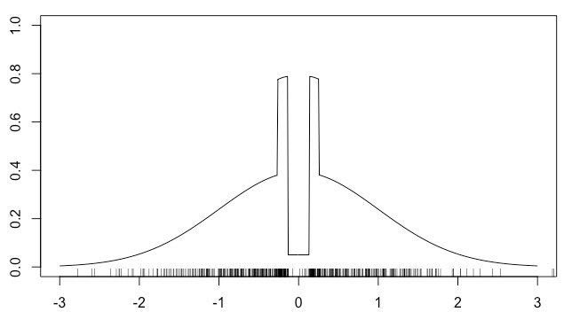
Figure 6: The density $f$ defined in (7) with a rug plot of a random sample of size $n=500$.

Einmahl et al. (2010a) motivated the shorth plot in part by demonstrating the shortcomings of standard techniques like the histogram or kernel density estimation in distinguishing this density (and its antimode) from a standard normal density based on a random sample. Just as the DQF $q_{x}(\delta)$ is related to the probability measure of an interval of size $\delta$ for which $x$ is the “median”, the shorth, $S_{\lambda}(x)$, also relates the length of a particular interval with its probability content, specifically

$$S_{\lambda}(x)=\inf\{|I|:P(I)\geq\lambda,I\in\mathcal{I}_{x}\},$$

where $\mathcal{I}_{x}$ is the class of intervals containing the point $x$. A similar approach was considered by Lientz (1974), where the set ${\cal I}_{x}$ was the set of intervals with midpoint $x$. Empirical versions are found by again replacing the probability measure with its empirical counterpart.

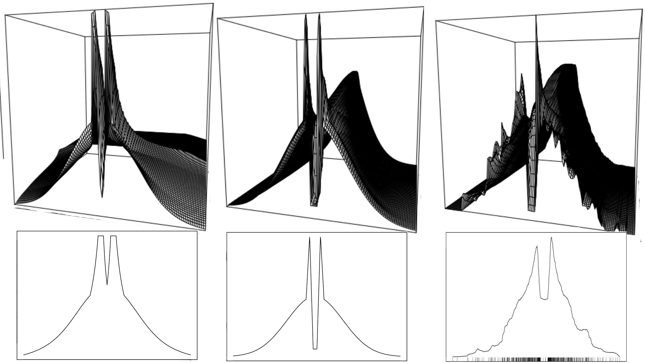
Figure 7: (left) reciprocal of the shorth over all $\lambda$; (middle) DQF over all $\delta;$ (right) estimated DQF based on a sample of size $n=500$, smoothed over $\delta$. All have been scaled at each $\lambda(\delta)$ to aid in visualization. Bottom shows individual slices at individual values of the scale parameter.

The shorth-plot was introduced as a function in $x$ for a given parameter $\lambda$ in Sawitzki (1994). The shorth-process considered in Einmahl et al. (2010b) is studied as a process in both $x$ and $\lambda$. The DQF is defined as a function in the parameter $\delta$ for each fixed $x,$ but of course for $d=1,$ it can also be plotted as a function in $x$. Figure 7 provides plots of these functions in both $x$ and the corresponding parameter. To make them comparable, we plot the reciprocal of $S_{\lambda}(x)$ (left figure), in addition to normalizing each plot such that, for a fixed value of the scale parameter, the integral over $x$ is 1. This means that for small parameter values, both functions (in $x$) might be considered as some type of density estimator. However, neither of these approaches is to be understood as such. Indeed, particularly in high dimensions when the curse of dimensionality kicks in, we are aiming at extracting more structural information in the sense of feature extraction.

One notable feature is that, in the low density “hole”, the shorth is “v”-shaped, while the DQF (both population and smoothed empirical versions) is “u”-shaped, matching the underlying density. To see why this is, consider the point $x=0.10$, which exists in the “hole”, though near its right hand boundary of 0.13. The interval of length 0.15 for the DQF will be approximately (-0.015, 0.135), almost entirely in the “hole,” and something similar will be true for any $x$ value in the “hole.” Meanwhile, the interval of the same length that will be considered by the shorth will be (0.1, .25) (corresponding to $\lambda$=0.095). Thus, as $x$ nears the boundary of the “hole,” the intervals instead increasingly resemble the intervals of non-anomalous points, masking the hole and resulting in the observed “v” shape.

A second feature of Figure 7 is that, for large $\lambda$, the information quality tends to degrade as $\lambda\to 1$, since $S_{1}(x)=|{\rm supp}(F)|$ for all $x$. This is in contrast to the DQF, which, by Lemma 2.1 yields information about the centrality of $x$ for large $\delta$. While visualizations of the type contained in Figure 7 will not be possible beyond the univariate set-up, the realization that valuable information is contained at both extremes of $\delta$ motivates plotting the DQF for each data point as a function of $\delta$, which will be possible for data of any dimension, as seen below.

4 Anomaly detection for $\mathbf{d}\boldsymbol{\geq}\mathbf{2}$ and object data

In this section numerical studies of the (a)DQF approach to anomaly detection are presented and discussed. We fix the cone angle $\alpha=\pi/4$ unless mentioned otherwise. We also drop the axis from the plots of the DQFs and their derivatives, because the scale is not of importance for our discussion. Recall that as described in subsection 2.3 (see Uniform distribution (iii)), the non-adaptive DQF uses the same (uniform) distribution $G_{ij}$ for all $i,j$.

4.1 Anomaly detection for multivariate Euclidean data

In low dimensional situations, using the observations themselves as anchor points may make sense. For instance, this would be beneficial in trying to detect the hole in a bivariate “rotated” version of (7). However, as the dimension of the data increases, issues related to the curse of dimensionality arise. A particularly salient one for the current method is that the fraction of points living on the boundary of the convex hull increases in dimension (Rényi and Sulanke, 1963). Points living on this boundary will tend to have very small half space depth. As half space depth underlies the construction of the depth quantile functions, in high dimensions the DQF for a large quantity of points will have nearly identical behavior, which empirically has been seen to be functions that only take on the values 0 and $1/n$. Thus, the ability to recognize anomalous observations is hampered. This provides rational for using $m_{ij}=\frac{x_{i}+x_{j}}{2}$ as our anchor points. Beyond having the aforementioned benefit of relating to antimodes for anomalous observations, these points are very likely to live in the interior of the convex hull and thus return informative (a)DQFs. Each observation is then associated with the averaged (a)DQF over midpoints formed between itself and other observations. Considering midpoints has the additional benefit of reducing the computational complexity of the algorithm, from $n(n-1)$ comparisons when the observations themselves are the “anchor points” to ${n\choose 2}$ when using midpoints. In the applications that follow, the averaged (a)DQFs are based on a random sample of 50 pairs rather than all pairs of points, further reducing the computational burden of the method.

A common feature of high dimensional data is the so-called manifold hypothesis (Fefferman, et al. 2016) that posits that the data often lives (at least approximately) on a manifold of much lower dimension than the $d$-dimensional ambient space. This fact is often exploited by dimension reduction algorithms, either linear (for instance, principal component analysis) or non-linear (for instance, Isomap by Tenenbaum, et al. 2000). Certainly an observation far in the tails of the point cloud might be considered anomalous, and this is the higher dimensional analog of what the box plot is designed to detect. Considering a definition of an outlier as an observation that is generated according to a different mechanism from the rest of the data set, such a point may lie off of the manifold, despite otherwise living “near” the point cloud (with respect to the ambient space).

A particular benefit of the DQF approach is adaptivity to sparsity. Suppose that the non-anomalous data lives in a $d^{\prime}$ dimensional affine subspace of the ambient space with dimension $d$, $d^{\prime}<d$. For any two non-anomalous points, the line $\ell_{ij}$ will also live in this subspace, and the intersection of our $d$-dimensional cones with this subspace will be cones of dimension $d^{\prime}$. In other words, the DQF approach will behave as if we had done appropriate dimension reduction beforehand.

In the following empirical studies, we use midpoints as anchor points, i.e. $m_{ij}=\frac{x_{i}+x_{j}}{2}.$ The aDQF uses a normal base distribution, centered at $m_{ij}$ with variance proportional to the $(\frac{n-6}{n})100\%$-Windsorized variance of the projected (onto $\ell_{ij}$) data. In the Euclidean case, the data is first $z$-scaled.

While the DQF approach results in a functional representation of each observation, a particularly informative region of these functions is for $\delta$ small, particularly the range of $\delta$ for which $\bar{q}(\delta)$ is 0. Considering the zero interval of the (a)DQFs means to look for “large distance gaps,” measured by $\delta_{x,y}$ (see Lemma 2.2). Of course, Lemma 2.1 also makes clear that $\delta$ small is related to the underlying density, resulting in somewhat of a unification of the two standard types of outliers, those far from the bulk of the data and those lying in low-density regions, even in the case of micro-clusters. To explore the sense in which the DQF approach to measuring distance gaps can facilitate anomaly detection, we contrast the DQF approach to stray (Talagala et al, 2021), an extension of the HDoutliers algorithm (Wilkinson, 2017), a well-studied and popular anomaly detection method based on the distribution of the $k$-nearest neighbors distances, specifically for anomalies defined by large distance gaps. We note that for an underlying manifold structure, an outlier lying off the manifold may have a small distance gap with respect to Euclidean distance in the ambient space, but a large distance gap with respect to a Mahalanobis-type distance with respect to the distribution on the manifold. We argue that the DQF approach, and particularly the aDQF, is sensitive to this type of anomaly and implicitly recognizes the large distance gap relative to a notion of distance based on the underlying geometry without the need for manifold learning.

4.1.1 Simulation Study

Consider the following example: 100 observations live on a 2-manifold defined by $y_{3}=2\cos((y_{1}-.5)\pi)$ with $(y_{1},y_{2})$ uniform in the unit square. A single observation lives at the point (0.5,0.5,1.5), so that the manifold is curving around this observation. This point cloud is then embedded in $d=30$ via a random linear map with matrix coefficients chosen uniformly on (-1,1) to form the data set we consider. Figure 8 shows the manifold in 3 space before mapping to the higher dimensional space, as well as the corresponding normalized aDQFs $\tilde{q}_{i}(\delta)$’s. The function corresponding to the outlying observation differentiates itself from the bulk of the data, including but not limited to a long zero interval. For this data set, the stray algorithm ranks the true outlier as the $3^{nd}$ most unusual point out of 101 (using oracle value of tuning parameter of $k=1$). The most outlying point according to stray corresponds to the function that is the smallest for intermediate values of $\delta$ in the figure. The corresponding point lies on the manifold, though in a region of the manifold which is sparse with respect to the given random sample.

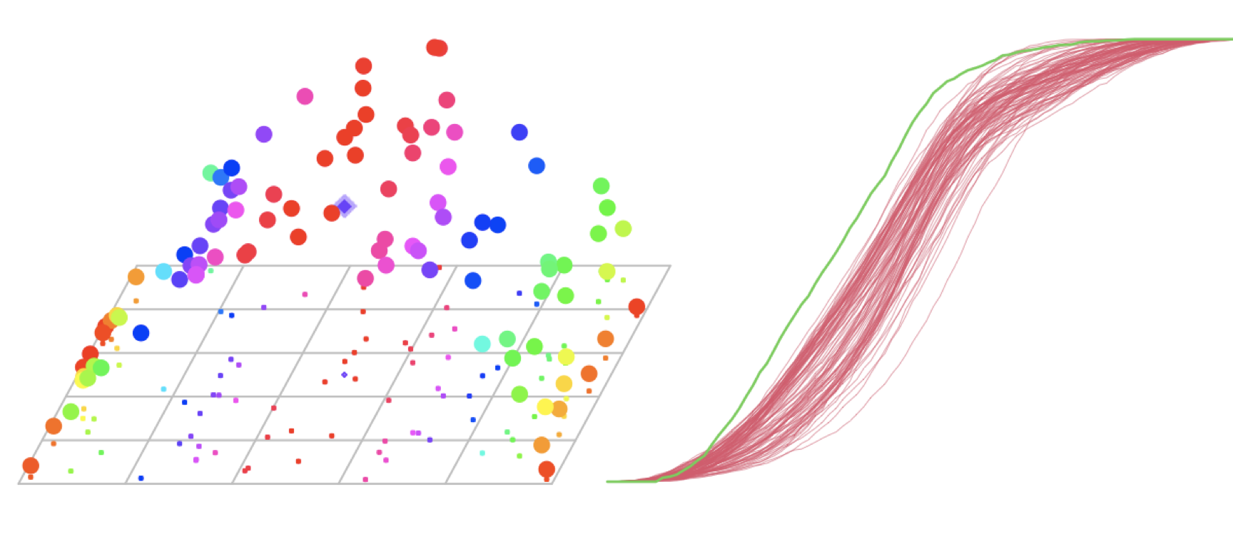
Figure 8: $x_{1},\ldots,x_{100}$ living on a 2-manifold embedded in $d=30$ with $x_{101}$ living off the manifold. (left) Data before mapping to ambient space, color coded by vertical height, outlier as diamond 0.5 below the apex of manifold, with rug plot (right) Normalized aDQFs $\tilde{q}_{i}(\delta)$ with outlier in green. The function living primarily below the bulk of functions corresponds to the non-anomalous blue-green point in the relatively sparse region of the manifold whose projection appears in the upper left.

As a more rigorous comparison, we simulated from several different models for high dimensional data with a single anomaly added to the point cloud. Our evaluation criterion is the rank of the true outlier according to the three methods. The rank of the outlier for the (a)DQFs corresponds to the rank at the smallest $\delta$ such that $\arg\min_{i}\bar{q}_{i}(\delta)$ is unique. Doing this ignores the multi-scale nature of the method. Indeed, we have seen in Figures 1 and 8, the most compelling information may be for $\delta$ away from 0, and in the case of anomalous micro-clusters as seen in Figure 1, the distance gap is actually smallest for the anomalous observations. However, in this study we explore isolated anomalies and thus rely on Lemma 2.2 and use small values of $\delta$. For stray, rank is based on the value of the outlier score, optimized over the parameter $k$. Table 1 contains results for the simulation set-ups, which we describe here.

The first model generates $(Y_{1},Y_{2})\sim U(0,1)^{2}$. A sample size of $n=80$ is then embedded in $d=50$ space again via a random linear map. A single observation is modified by adding a vector orthogonal to the plane with norm 0.4, that now constitutes the outlier. (Both the observation and the orthogonal vector are selected randomly.) The second simulation generates $n=100$ points uniformly in the 6-dimensional unit hyper-cube before embedding it into an ambient space of $d=100$ in the same manner as above. Noise is then added of the form $\epsilon\sim{\rm MVN}(0,.05^{2}I)$. The outlier is again generated by adding a vector, orthogonal to the 6 dimensional hyperplane, now with norm 10, to a single observation. The third simulation generates 100 points on the non-linear manifold described above, with a $101^{st}$ at (.5,.5,1) prior to being mapped into the ambient space of $d=30$. Finally, we compare the two methods outside of a manifold structure. To this end, $n=50$ multivariate standard normal draws are taken in $d=30$. To obtain an outlier, the first component is set to 6 for a single observation.

In all cases, the aDQF outperforms the ranks provided by stray according to both metrics considered. Furthermore, the aDQF outperforms the non-adaptive version in all simulations where the manifold hypothesis held true. Interestingly, in a similar simulation to the $3^{rd}$ one above, it was very uncommon for a given data set to confuse both methods, suggesting that the information used in the DQF is quite different to the distances used by stray, see table 2. Finally, improved results were observed for the aDQF using a normal base distribution $G_{ij}$ versus a uniform. For instance, in the 6 dimensional subspace example, a uniform $G_{ij}$ with support proportional to the Windsorized standard deviation identified the outlier correctly only 46% of the time.

$d$	$d^{\prime}$	$n$	DQF	aDQF	stray
50	2	80	0.994 (1.01)	0.998 (1.00)	0.60 (1.79)
100	6 + noise	100	0.39 (3.49)	0.91 (1.12)	0.22 (4.2)
30	2 (non-linear)	101	0.93 (1.22)	0.97 (1.07)	0.67 (1.50)
30	30	50	0.54 (2.76)	0.54 (2.80)	0.20 (8.82)

Table 1: Simulation results comparing DQF, aDQF and stray for $d^{\prime}$ dimensional data embedded in a $d$ dimensional ambient space. One outlier present in all cases. Results are proportion of simulations where outlier is identified as most outlying observation (average rank of true outlier).

	Correct	Incorrect
Correct	932	42
Incorrect	23	3

Table 2: Simulation results for a noisy version of the non-linear manifold example. Outlier is $x_{101}=(0.5,0.5,0)+MVN(0,.05^{2}I)$.

4.1.2 Real Data

As a real data example, we consider the multiple features data set available at the UCI Machine Learning Repository (https://archive.ics.uci.edu/). The data set consists of $d$=649 features of handwritten digits, with 200 observations for each digit. This data set was considered in Chandler and Polonik (2021), where a data set consisting of all “6” and “9” observations were contaminated with 20 “0”s. Figure 9 considers all 200 “4” digits and the first five “5” digits in the data set. The DQFs again use midpoints as anchor points. The 5 anomalous observations clearly separate themselves out from the rest of the data, whereas stray assigns ranks 2,3,4,10 and 11 to them. For the anomalies, flat parts away from $\delta=0$ are observed, as discussed in section 2.2.2. These are due to the five anomalies being the only observations in the $A$-sets for a large range of cone tips. This behavior also suggests that the manifold comprising the non-anomalous support curves around the five outliers, similar to what is illustrated in figure 5. The curvature of this manifold is seemingly the reason that the visual information in the non-adaptive DQF presented here is better than the aDQF.

Next, we consider a data set of size $n=210$, consisting of all “5” observations and the first 10 “9” observations. Based on the visually chosen 0.42 quantile, the area under the response operator curve (ROC AUC) is 0.97 (0.989 if based on the normalized DQF), compared to 0.915 for stray. Comparing all 200 “6” observations to the second 10 “9” observations yielded an AUC of 0.975 versus 0.95 for stray.

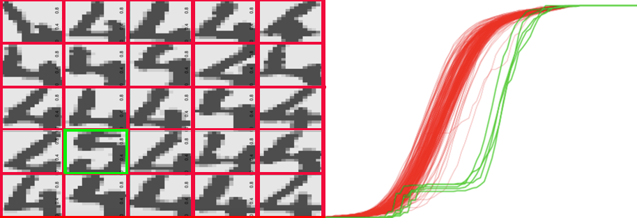
Figure 9: Normalized DQFs $\tilde{q}_{i}(\delta)$ from the multiple features data set. 200 “4” digits (red) and the first 5 “5” digits (green).

4.2 Object Data - Kernelized DQF

Given that the (a)DQF only requires computing distances between observations, any object data for which a kernel function is defined can be visualized by using the corresponding Reproducing Kernel Hilbert Space (RKHS) geometry via the (a)DQF. Here we consider three such examples.

In each of the following examples, the data itself can be visualized, unlike the previous Euclidean data settings. However, the (a)DQF, guided by Lemma 2.2, provides a visualization that structures the data according to its outlyingness, facilitating identification that may be difficult when observing the raw data. We begin by consider Example 1 from Nagy and Hlubinka (2017). We generate 100 functions of the form $X(t)=A+B\arctan(x)+G(t)$, with $A\sim N(0,4)$, $B\sim{\rm Exp}(1)$ and $G(t)$ a zero-centered Gaussian process with covariance function $k(s,t)=0.2e^{\frac{-|s-t|}{0.3}}$, $0<s,t<1$. These constitute the non-anomalous observations, while a $101^{st}$ observation generated as $Y(t)=1-2\arctan(t)+G(t)$ forms the anomaly, off the manifold bounded by $B=0$. Figure 10 shows both the raw data and the aDQF based $L_{2}$-inner product.

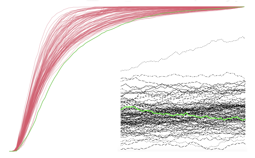
Figure 10: Functional data example, raw data (inset) and normalized aDQF $\tilde{q}_{i}(\delta)$. The anomaly (green) tends to decrease while the non-anomalous observations tend to increase. The other observation identified by the aDQF corresponds to the highest function.

The second example is the shape classification task studied in Reininghaus et al. (2015), where we analyze 21 surface meshes of bodies in different poses, in particular the first 21 observations of the SHREC 2014 synthetic data set. The first 20 correspond to one body, while the $21^{st}$ corresponds to a different body, which we regard as an outlier.

The approach to compare these surface meshes consists of various steps that we now briefly indicate. The first step is to construct the so-called Heat Kernel Signature (HKS) for each of the surface meshes. The HKS is a function of the eigenvalues and eigenvectors of the estimated Laplace-Beltrami operator (see Sun et al., 2009). One can think of the HKS as a piece-wise linear function on the surface mesh, whose values reflect certain geometric aspects of the surface. This piece-wise linear function is constructed by first defining function values $h_{t}(v_{i})$ on all the vertices $v_{i},i=1,\ldots,N$ (where $t$ is a tuning parameter), and then finding the function value at each face $f_{j}$ of the mesh as $h_{t}(f_{j})=\max_{v_{i}\in f_{j}}h_{t}(v_{i})$. The values $h_{t}(v_{i})$ have the form $h_{t}(v_{i})=\sum_{k=1}^{N}e^{-\lambda_{k}t}\phi_{ik},$ where $\phi_{i}=(\phi_{i1},\ldots,\phi_{iN})$ is the $i$-th eigenvector of a normalized graph Laplacian. For more details we refer to Belkin et al. (2008). Comparing these functions directly is not possible, because they live on different surfaces. Thus, certain features of these functions are extracted. This is accomplished by constructing a persistence diagram for each of the HKSs, using their (lower) level set filtration. We refer to Chazal and Michel (2021) or Wasserman (2018) for introductions to persistent homology, including persistence diagrams. In a nutshell, these persistence diagrams measure the number of topological features of the level sets of the HKSs along with their significance (persistence), which in turn is related to the heights of the critical points of the functions. In particular, it is not a single level set that is considered, but the entire filtration of level sets. Persistence diagrams are multisets of 2-dimensional points, and thus one is faced with comparing such 2-dimensional point sets. To this end, one can use the kernel trick to implicitly map the persistence diagram into a RKHS and use the corresponding RKHS geometry in our DQF approach. The kernel we are using is the persistence scale-space kernel (PSSK) $k_{\sigma}$ of Reininghaus et al. (2015). Based on this we construct the Gram matrix on which the aDQF is based, with the resulting aDQF plot shown in Figure 11, which provided stronger visual evidence than the non-adaptive DQF.

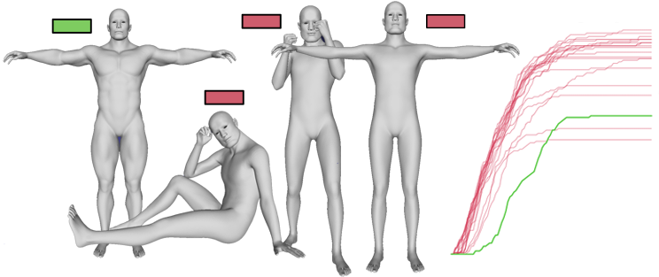
Figure 11: aDQFs $\bar{q}_{i}(\delta)$ based on a kernel defined on persistence diagrams. Red lines correspond to 20 poses of one body, green line corresponds to a single pose of a different body (outlier). Tuning parameters of $t=500$ for the HKS and $\sigma=1$ for the PSSK were used.

Our third example in this subsection is considering gerrymandering. We follow the techniques of Duchin, et al. (2021) to compute a persistence diagram based on a graph representation of districting maps filtered by Republican vote percentage in the 2012 Pennsylvania Senate election. Again one can think of these persistence diagrams being constructed by first constructing a function over each potential districting map. This is accomplished by associating each districting map with a graph (vertices are the districts; edges are placed between vertices if the districts physically share a part of their boundary). Then, a function is constructed over this graph, by defining a function value at each vertex (district), which is given by the portion of Republican votes (based on counts of precincts at a given election). Then, as in our previous example, one constructs a persistence diagram for this function by again using its level set filtration. This is done for both the 2011 map invalidated by the Supreme Court for partisan gerrymandering as well as random maps generated according to the ReCom algorithm (Deford, et al. 2021). The idea is that these randomly chosen districting maps constitute a representative sample of maps, and they are being used to answer the question of whether the gerrymandered map is an anomaly.

In our analysis, the aDQFs were again computed using the kernel trick via PSSK, resulting in a visualization of the extent at which the 2011 map is anomalous, see Figure 12.

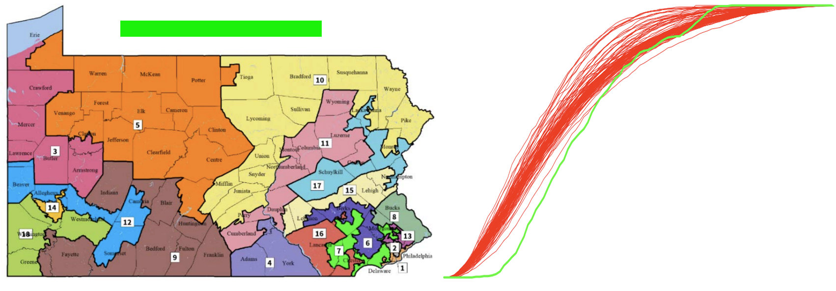
Figure 12: Normalized aDQFs $\tilde{q}_{i}(\delta)$ based on a kernel defined on persistence diagrams. Red lines correspond to 99 randomly generated districting maps via ReCom, green corresponds to 2011 map (pictured, source: https://ballotpedia.org/) invalidated by the Supreme Court in 2018 for partisan gerrymandering.

5 Implementation

The computational complexity of the method is somewhat high, due primarily to the construction of a matrix of feature functions, as pairs of points are considered. Since we are not working with these individual functions directly but rather their averages, we propose basing these averages on only a subset of these pairwise comparisons. For a fixed number of comparisons, this allows the complexity to grow linearly in the sample size rather than quadratic. The algorithm is also embarrassingly parallel.

We propose using three visualizations of the (a)DQFs, the averaged (over a random subset) $\bar{q}_{i}(\delta)$, its normalized (by the maximal value) version, $\tilde{q}_{i}(\delta)$, and the first derivative of the normalized version $\frac{d}{d\delta}\tilde{q}_{i}(\delta)$ (after a small amount of smoothing), at multiple values of $\alpha$ (which as discussed above, does not add much computational complexity to the algorithm). The functions dqf.outlier and dqf.explore in the R package dqfAnomaly generate and visualize these three functions as interactive plots in base-R.

For instance, the 30-dimensional simulation data demonstrates the need to consider multiple angles. For sufficiently high dimension, there is likely to exist a range of $\delta$ such that $\widehat{q}_{ij}(\delta)=\frac{1}{n}$ for all $i,j$, as these cones will only include the two points $x_{i}$ and $x_{j}$ that define the direction. This is apparent in Figure 13 at angle $\alpha=\pi/6$.

As a real data example, we consider the wine data, commonly used for illustrating classification algorithms and available at the UCI Machine Learning Repository (https://archive.ics.uci.edu/). The data set was subsampled by considering all 59 class 1 observations and 3 random points from other classes (observations 122, 153, and 164 from the full data set) to see if it is possible to detect these three anomalous observations. The functions above generate the plots shown in the right panel of Figure 13. All three outliers differentiate themselves from the fairly homogenous aDQFs corresponding to the class 1 observations.
Rather than consider the current method as competing with existing outlier detection algorithms, we rather view the (a)DQF as complementary. It’s clear from the simulation studies and real data examples that both the (a)DQF and stray are effective at identifying anomalous observations. Many other effective techniques exist as well. Due to the computational complexity of computing the (a)DQF (mainly with respect to sample size), identifying a suitable subset of the data to visualize via a more computationally friendly method such as stray for very large data sets would ease the computational burden. That is, one can compute the (a)DQF of a random subset of non-anomalous observations and any identified interesting observations to create a useful visualization of subsets of the data.

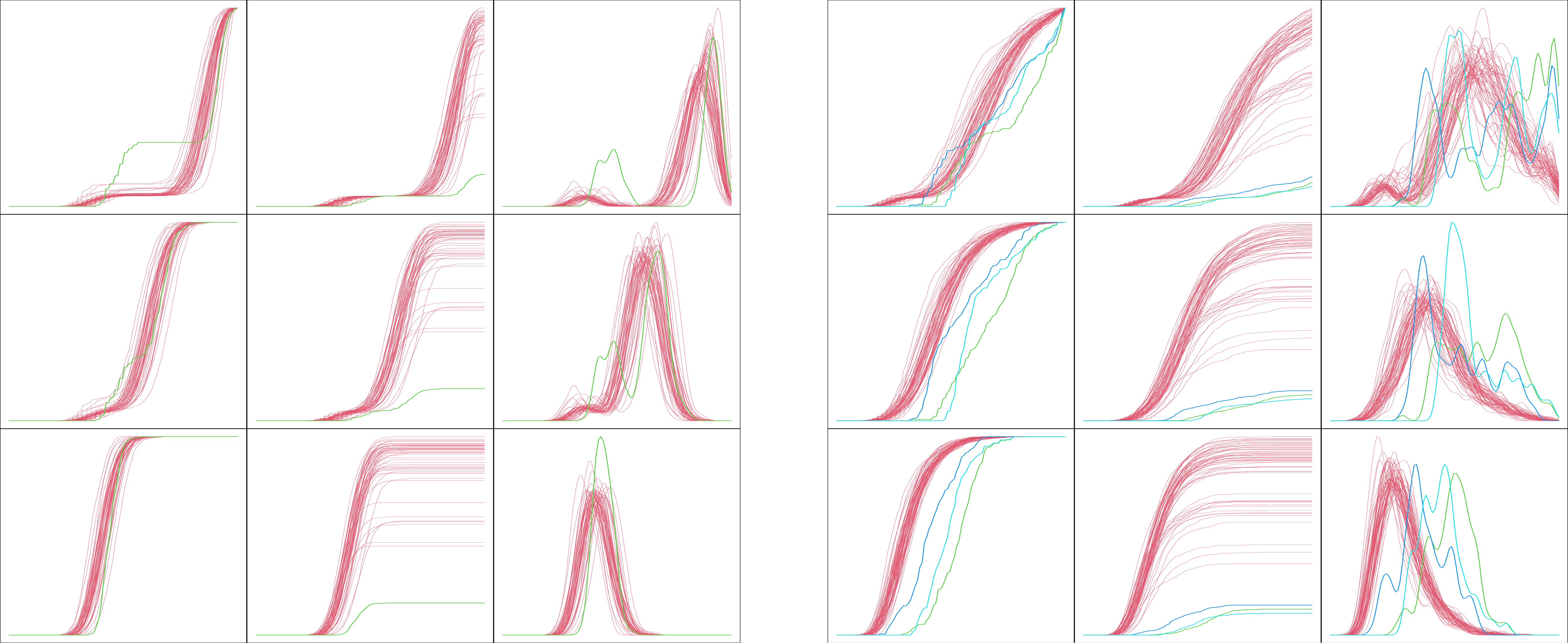
Figure 13: Visualization of (left column) normalized aDQFs $\tilde{q}_{i}(\delta)$, (center column) raw averaged aDQFs $\bar{q}_{i}(\delta)$ and (right colum) first derivative of normalized aDQF $\frac{d}{d\delta}\tilde{q}_{i}(\delta)$ for the (left panel) $d=30$ simulation data and the (right panel) subsampled wine data. Outliers indicated by color. Rows correspond to different angles ($\alpha=\pi/6,\pi/4,\pi/3$).

6 Technical proofs.

Proof of Lemma 2.1. We present the proof for the case $G=U[0,1]$. The extension to more general $G$ is straightforward.

By definition of $d_{x}(s)$ (see (1)), we have that $d_{x}(s)$ is continuous, $d_{x}(x)=0$, and $d_{x}(s)$ is non-decreasing for $s\in[x,1]$ and non-increasing for $s\in[0,x].$ Thus for each $0\leq t\leq 1$ there exist $0\leq a_{x}(t)\leq b_{x}(t)\leq 1$ with $\{s:d_{x}(s)\leq t\}=[a_{x}(t),b_{x}(t)].$ Let $S\sim G=U(0,1).$ The random depth that we are considering here is $d_{x}(S)$, and its cdf is

$$D_{x}(t)=P(d_{x}(S)\leq t)=b_{x}(t)-a_{x}(t).$$ (8)

We further have $D_{x}(TD(x,F))=1,$ and with $\delta_{x}^{*}$ given in (4),

$$\lim_{t\nearrow{\rm TD}(x,F)}D_{x}(t)=\delta^{*}_{x}.$$ (9)

To see (9), simply find the smallest value $s^{*}$ for which $d_{x}(s^{*})$ attains its maximum ${\rm TD}(x,F)$. Then, the limit in (9) equals $s^{*}$ in case $s^{*}>x$, and $1-s^{*}$ for $s^{*}<x.$ To find $s^{*}$ for $x$ with $F(x)<\frac{1}{2}$ (i.e. ${\rm TD}(x,F)=F(x)$), note that $d_{x}(s)<F(x)$ for $s<x$, so that $s^{*}>x$. So we simply find $s^{*}$ by solving $F(s^{*})-F(x)=F(x)$ (see (1)), which gives $s^{*}=F^{-1}(2F(x))$. The case $F(x)>\frac{1}{2}$ is similar. If $F(x)=\frac{1}{2}$ then there is no value $s^{*}$ for which $d_{x}(s^{*})={\rm TD}(x)$, and in this case the limit in (9) equals 1, which immediately follows from (1). So unless ${\rm TD}(x)=\frac{1}{2},$ i.e. unless $x$ is the median of $F$, the function $D_{x}(t)$ has a discontinuity at $t={\rm TD}(x).$

Another needed observation is the following. Recall (see (8)) that $D_{x}(t)$ equals the length of an interval (the sublevel set of $d_{x}(s)$ at level $t$). Given such a a sublevel set $[a,b]$ of length $\delta<\delta_{x}^{*},$ the values of $d_{x}(s)$ at the boundaries of this interval are $d_{x}(a)=F(a)-F(x)$ and $d_{x}(b)=F(x)-F(b)$, respectively. Since $[a,b]$ is a sublevel set of $d_{x}(s)$, these values need to be equal to the corresponding level, and their sum equals $F(b)-F(a)$, the probability content of the interval. In other words, the level corresponding to a sublevel set of length $\delta<\delta^{*}$ equals half of the probability content of the sublevel set. Since

$$q_{x}(\delta)=\inf\{t:D_{x}(t)\geq\delta\},$$

the above arguments now give that $q_{x}(\delta)$ reaches its maximum value $TD(x,F)$ at $\delta^{*}_{x}$. Now let $\Delta_{x}$ be the set of all the lengths of the sublevel sets $d_{x}(s)$, i.e. $\Delta_{x}=\{\delta\in[0,1]:\,\exists\,t_{\delta}\;\text{\rm with }\,D_{x}(t_{\delta})=\delta\}$. For $\delta\in\Delta_{x}$ with $\delta<\delta^{*}_{x},$ we have $q_{x}(\delta)=t_{\delta}$, and the above arguments imply that $q_{x}(\delta)=t_{\delta}=\frac{1}{2}F(a_{x,\delta},b_{x,\delta}]),$ where $a_{x,\delta}=a_{x}(t_{\delta})$ and $b_{x,\delta}=b_{x}(t_{\delta})$.

It remains to show (5) for values of $\delta\in[0,1]\setminus\Delta_{x}$. They correspond to levels $t_{\delta}$ at which the cdf $D_{x}(t)$ is not continuous, or $q_{x}(\delta)$ has a flat part. More precisely, for $\delta\in[0,1]\setminus\Delta_{x}$, let $\delta_{u}=\inf\{\gamma\in\Delta_{x}:D_{x}(t_{\gamma})\geq\delta\}$ and $\delta_{\ell}=\sup\{\gamma\in\Delta_{x}:D_{x}(t_{\gamma})<\delta\}$. Then, $\delta_{\ell}\leq\delta\leq\delta_{u}$ (with at least one of the inequalities being strict). For any sequence $\{\delta_{m}\}\subset\Delta_{x}$ with $\delta_{m}\searrow\delta_{u}$, the corresponding sequence $t_{\delta_{m}}=\frac{1}{2}F([a_{x}(t_{\delta_{m}}),b_{x}(t_{\delta_{m}})])$ converges to $t_{\delta},$ and the intervals $[a_{x}(t_{\delta_{m}}),b_{x}(t_{\delta_{m}})]$ converge (the endpoints converge monotonically) to an interval $[a_{\delta_{u}},b_{\delta_{u}}]$ with $d_{x}(a_{\delta_{u}})=d_{x}(b_{\delta_{u}})=\frac{1}{2}F([a_{\delta_{u}},b_{\delta_{u}}])=t_{\delta}.$ Similarly, for $\{\delta_{m^{\prime}}\}\subset\Delta_{x}$ with $\delta_{m^{\prime}}\nearrow\delta_{\ell}$, the corresponding sequence of intervals $[a_{x}(t_{\delta_{m^{\prime}}}),b_{x}(t_{\delta_{m^{\prime}}})]$ converges to an interval $[a_{\delta_{\ell}},b_{\delta_{\ell}}]$ with $[a_{\delta_{u}},b_{\delta_{u}}]\subset[a_{\delta_{\ell}},b_{\delta_{\ell}}],$ and $t_{\delta}=\frac{1}{2}F([a_{\delta_{\ell}},b_{\delta_{\ell}}]).$ Geometrically, the function $d_{x}(s)$ has a flat part (is constant equal to $t_{\delta}$) on $A_{x}=[a_{\delta_{\ell}},b_{\delta_{\ell}}]\setminus[a_{\delta_{u}},b_{\delta_{u}}],$ where $A_{x}$ has strictly positive Lebesgue measure, but $F(A_{x})=0$. In particular, $x$ is the median for any interval $[a,b]$ with $[a_{\delta_{u}},b_{\delta_{u}}]\subset[a,b]\subset[a_{\delta_{\ell}},b_{\delta_{\ell}}].$ So, we have $q_{x}(\delta)=\frac{1}{2}F[a_{x,\delta_{u}},b_{x,\delta_{u}}]=\frac{1}{2}F[a_{x,\delta_{\ell}},b_{x,\delta_{\ell}}]=\frac{1}{2}F([a,a+\delta]).$ This completes the proof of (5).

To see the last assertion of the lemma, observe that

$$\lim_{t\searrow 0}D_{x}(t)=l_{x}.$$ (10)

In particular, this implies that for $x\notin{\rm supp}(F)$, $D_{x}(t)$ has a discontinuity at $t=0,$ and thus, for such values of $x$, the DQF $q_{x}(\delta)$ is constant equal to zero for $\delta\in[0,l_{x}].$

$\Box$

Proof of Lemma 2.2: By definition of $t^{\pm}_{x,y}$, we have $F\big{(}A_{x,y}(s)\big{)}=0$ for $s\in\big{(}m_{x,y}-t^{-}_{x,y}u,\,m_{x,y}+t^{+}_{x,y}u)\subseteq[a_{x,y},b_{x,y}].$ From this we have that $d_{x,y}(s)=\min\big{(}F(A_{x,y}(s),B_{x,y}(s)\big{)}=0.$ The $G_{x,y}$-measure of this set by definition equals $\delta_{x,y}.$ It follows that $q_{x,y}(\delta)=0$ for $\delta\in[0,\delta_{x,y}],$ and thus have $q_{x,y}(\delta)=0$ for all $\delta\in[0,\delta_{x,y}].$ This implies that $\overline{q}_{x}(\delta)=0$ for all $\delta\in[0,\inf_{y}\delta_{x,y}].$

$\Box$

7 References

Aggarwal, C.C. (2013): Outlier Analysis. Springer, New York.
Belkin, M., Sun, J. and Wang, Y. (2008): Discrete Laplace operator on meshed surfaces. In SCG ’08: Proceedings of the twenty-fourth annual symposium on computational geometry, 278 - 287.
Burridge, P., and Taylor, R. (2006): Additive Outlier Detection Via Extreme-Value Theory. J. Time Ser. Anal. 27. 685-701.
Chandler, G. and Polonik, W. (2021): Multiscale geometric feature extraction for high-dimensional and non-Euclidean data with applications. Ann. Statist. 49, 988-1010.
Chazal, F. and Michel, B. (2021): An introduction to topological data analysis: fundamental and practical aspects for data scientists. Front. Artif. Intell., 4.
DeFord, D., Duchin, M. and Solomon, J. (2021): Recombination: A Family of Markov Chains for Redistricting. Harvard Data Sci. Rev. 3.1
Duchin, M., and Needham, T. and Weighill, T. (2021): The (homological) persistence of gerrymandering. Found. Data Sci. 10.3934/fods.2021007.
Einmahl, J. H. J., Gantner, M., and Sawitzki, G. (2010a): The Shorth Plot. J. Comput. Graphical Stat., 19(1), 62-73.
Einmahl, J. H. J., Gantner, M., and Sawitzki, G. (2010b): Asymptotics of the shorth plot. J. Stat. Plann. Inference, 140, 3003–3012.
Fefferman, C., Mitter, S., and Narayanan, H. (2016): Testing the manifold hypothesis. J. Am. Math. Soc. 29, 983–1049.
Fisherkeller, M. A., Friedman, J. H. and Tukey, J. W. (1974): PRIM-9, an interactive multidimensional data display and analysis system. Proceedings of the Pacific ACM Regional Conference. [Also in The Collected Works of John W. Tukey V (1988) pp. 307–327.]
Friedman, J.H. and Stuetzle, W. (2002): John W. Tukey’s work on interactive graphics. Ann. Stat., 30, 1629-1639.
Hawkins, D. M. (1980): Identification of Outliers. Chapman and Hall, London – New York.
Huber, P.J. (1964): Robust estimation of a location parameter. Ann. Math. Stat., 35(1), 73–101.
Hyndman, R. J., (1996): Computing and graphing highest density regions. Am. Stat., 50, 120-126.
Hodge, V.J. and Austin, J. (2004): A survey of outlier detection methodologies. Artif. Intell. Rev., 22 (2), 85-126.
Lientz, B. P. (1974): Results on nonparametric modal intervals, SIAM J. Appl. Math, 19, 356-366.
Minnotte, M. and Scott, D. (1993): The Mode Tree: A Tool for Visualization of Nonparametric Density Features. J. Comput. Graphical Stat. 2, 51-68.
Nagy, S., Gijbels I., and Hlubinka, D. (2017): Depth-Based Recognition of Shape Outlying Functions, J. Comput. Graphical Stat., 26, 883-893.
Reininghaus, J., Huber, S., Bauer, U. and Kwitt, R. (2015): A stable multi-scale kernel for topological machine learning. IEEE Conference on Computer Vision and Pattern Recognition (CVPR), 4741–4748.
Rényi, A. and Sulanke, R. (1963): Über die konvexe Hülle von n zufällig gerwähten Punkten I. Z. Wahrsch. Verw. Gebiete, 2, 75–84.
Ruff, L., Kauffmann, J., Vandermeulen, R., Montavon, G., Samek, W., Kloft, M., Dietterich, T., and Müller, K. (2021): A Unifying Review of Deep and Shallow Anomaly Detection. Proceedings of the IEEE. 109(5), 1-40.
Sun, J., Ovsjanikov, M. and Guibas, L. (2009): A concise and probably informative multi-scale signature based on heat diffusion. Computer Graphics Forum, 28(5), 1383 - 1392.
Sawitzki, G. (1994): Diagnostic plots for one-dimensional data. In: Ostermann, R., Dirschedl, P. (Eds.), Computational Statistics, 25th Conference on Statistical Computing at Schloss Reisensburg. Physica-Verlag, Springer, Heidelberg, pp. 237–258.
Talagala, P.D., Hyndman, R.J. and Smith-Miles, K. (2021): Anomaly Detection in High-Dimensional Data, J. Comput. Graphical Stat., DOI: 10.1080/10618600.2020.1807997
Tenenbaum JB, de Silva V., and Langford JC. (2000): A global geometric framework for nonlinear dimensionality reduction. Science. 290(5500), 2319-23.
Tukey, J. W. (1975): Mathematics and the picturing of data. Proceedings of the International Congress of Mathematicians. 1975, pp. 523–531.
Wasserman, L. (2018): Topological data analysis. Annu. Rev. Stat. Appl., 5, 1501-532.
Wilkinson, L. (2017): Visualizing big data outliers through distributed aggregation. IEEE Trans. Visual Comput. Graphics 24(1), 256–266.