Computing nodal deficiency with a refined Dirichlet-to-Neumann map
Abstract.
Recent work of the authors and their collaborators has uncovered fundamental connections between the Dirichlet-to-Neumann map, the spectral flow of a certain family of self-adjoint operators, and the nodal deficiency of a Laplacian eigenfunction (or an analogous deficiency associated to a non-bipartite equipartition). Using a refined construction of the Dirichlet-to-Neumann map, we strengthen all of these results, in particular getting improved bounds on the nodal deficiency of degenerate eigenfunctions. Our framework is very general, allowing for non-bipartite partitions, non-simple eigenvalues, and non-smooth nodal sets. Consequently, the results can be used in the general study of spectral minimal partitions, not just nodal partitions of generic Laplacian eigenfunctions.
Key words and phrases:
Spectral flow, nodal deficiency, Dirichlet-to-Neumann operators, minimal partitions2010 Mathematics Subject Classification:
35P051. Introduction
Let be an open, bounded set, with piecewise boundary, and suppose is an eigenfunction of the Dirichlet Laplacian on , with eigenvalue . We denote by the nodal set of ,
and by the number of nodal domains of , i.e. the number of connected components of the set . We also let denote the minimal label of the eigenvalue , where are the ordered Dirichlet eigenvalues of , repeated according to their multiplicity. The Courant nodal domain theorem states that , or equivalently, that the nodal deficiency is nonnegative.
Letting denote the two-sided Dirichlet-to-Neumann map on , which will be defined below, we now state a special case of our main result.
Theorem 1.1.
The eigenfunction has nodal deficiency
| (1.1) |
and the corresponding eigenvalue has multiplicity
| (1.2) |
The symbol denotes the Morse index, i.e. the number of negative eigenvalues of the operator , which is self-adjoint and lower semi-bounded. A similar formula for the nodal deficiency appeared in [12]; see also [8]. The version of the Dirichlet-to-Neumann map appearing in the above theorem is more involved than the one used in [8, 12], but consequently gives us a stronger result, as we now explain.
We denote the nodal domains of by . When defining the Dirichlet-to-Neumann map, one must take into account that is a Dirichlet eigenvalue on each . Introducing the notation , we define the closed subspace
| (1.3) |
of , where denotes the restriction of to , is the restriction of to , and is the outward unit normal to . For sufficiently smooth , each boundary value problem
| (1.4) |
has a solution . Defining a function on by
| (1.5) |
for all , we let
| (1.6) |
where denotes the -orthogonal projection onto the subspace .
The solution to the problem (1.4) is non-unique, but the choice of particular solution is irrelevant for the definition on account of the projection in (1.6). In Theorem 3.1 we use this freedom to give an equivalent formulation of the Dirichlet-to-Neumann map that does not involve .
The earlier works [8, 12] avoided the difficulty of defining the Dirichlet-to-Neumann map at a Dirichlet eigenvalue by evaluating the quantities in Theorem 1.1 at , with a small positive . The resulting expression for the nodal deficiency was
| (1.7) |
Unlike (1.1), which immediately implies , the equality (1.7) only yields the same conclusion if we know that is simple, or have additional information about the spectrum of . Therefore, we obtain a more useful result by computing the Dirichlet-to-Neumann map at instead of .
An even stronger motivation for eliminating the -perturbation is that the unperturbed operator appears naturally as the Hessian of the energy functional on the space of generic equipartitions [7]. The minima of this functional are spectral minimal partitions, as defined in [17], which are often non-bipartite (unlike the decompositions of into nodal domains of an eigenfunction , mentioned above). One of the simplest examples of a non-bipartite partition is the so-called Mercedes star partition, which is an (unproven but natural) candidate for the minimal -partition of the disk; see [11] and references therein. The main result of this paper, Theorem 1.7, is a generalization of Theorem 1.1 to partitions that are not necessarily bipartite, but have certain criticality properties that make them prime candidates for being minimal.
We first recall111Here we are following the convention of [18]; in [11, 17] such a is called a strong partition. that a -partition of is a family of mutually disjoint, open, connected subsets of , with . We say that the subdomains and are neighbors if . We also recall that is bipartite if we can color the partition with two colors in such a way that any two neighbors have different colors. Defining the boundary set of the partition to be
| (1.8) |
we next impose a suitable regularity assumption on .
Definition 1.2.
A partition is said to be weakly regular if its boundary set satisfies:
-
(i)
Except for finitely many critical points , is locally diffeomorphic to a regular curve. In a neighborhood of each , is a union of smooth half-curves with one end at .
-
(ii)
consists of a finite set of boundary points . In a neighborhood of each , is a union of distinct smooth half-curves with one end at .
-
(iii)
The half-curves meeting at each and are pairwise transversal to one another, and to .
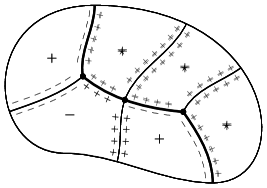
The subdomains are only allowed to have corners at points where at least three subdomains meet, or on . However, the definition still allows for partitions where a subdomain is a neighbor of itself, as shown in Figure 1.1. To rule out such examples, we say that a partition is two-sided222In [11] such partitions are said to be nice. We prefer the term two-sided, as it conveys the fact that each smooth component of is contained in the boundary of two distinct subdomains. if for each . For the rest of the paper we will only consider two-sided, weakly regular partitions. This is a reasonable hypothesis, as it is satisfied by nodal partitions, and more generally by spectral minimal partitions [10, 17].

For a two-sided, weakly regular partition each is a Lipschitz domain, so we can define trace operators and solve boundary value problems in a standard way. Without the transversality condition (iii) the may have cusps, and the analysis becomes much more difficult; see, for instance [5]. If the partition is not two-sided, then some lies on both sides of its boundary. In this case it is possible to define separate trace operators on each side of the common boundary; we do not to this here, but refer to [15, Section 1.7] for an example of this construction.
To extend the notion of a “nodal partition” to partitions that are not necessarily bipartite, it is convenient to introduce a generalization of the Laplacian. The construction involves a choice of signed weight functions, which will also be used to define a generalized two-sided Dirichlet-to-Neumann map on the partition boundary set.
Definition 1.3.
Given a two-sided, weakly regular partition , let
| (1.9) |
We say that functions are valid weights if they are constructed as follows. Given an orientation of each , and an orientation of each smooth component of , we define on each smooth component of to be if the orientation of agrees with the orientation of the corresponding smooth component of , and equal to otherwise.
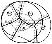
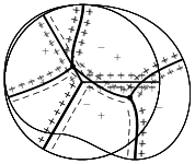
In Figure 1.2 we illustrate the construction of a valid set of weights, and also give an example of a non-valid choice of weights. Note that is constant on each smooth segment of ; the value at the corner points is irrelevant. According to Definition 1.3, there are two ways can change sign on : 1) it can change sign at a corner; or 2) it can take different signs on different connected components. It is easily shown that a partition is bipartite if and only if the weights are valid, cf. [7, Lemma 9], and so non-constant weights are essential for the study of non-bipartite partitions.


Remark 1.4.
An equivalent construction of valid weights can be given in terms of a co-orientation of each and each smooth component of . Along each we choose a vector field that is equal to either or . Choosing a vector field that is a smooth unit normal to each smooth component of , we set . A special case of this construction appeared in [7], where was chosen to be the outward unit normal , in which case whenever and are neighbors. The extra flexibility in the present construction will be useful below, in our discussion of -nodality.
Valid weights have a natural geometric interpretation in terms of the cutting construction in [18, Section 4], where one removes a portion of the nodal set from the domain in such a way that the resulting partition of is bipartite; see Appendix A for details.
We now introduce a weighted version of the Laplacian, , corresponding to the bilinear form defined on the domain consisting of such that
| (1.10) | |||||
| (1.11) | |||||
| (1.12) |
and given by
| (1.13) |
The Laplacians for different valid weights will be shown in Proposition 2.6 to be unitarily equivalent. As a consequence, if the partition is bipartite, then is unitarily equivalent to the Dirichlet Laplacian on . Furthermore, the nodal sets of the eigenfunctions of are independent of , justifying the following definition.
Definition 1.5.
A two-sided, weakly regular partition is said to be -nodal if it is the nodal partition for some eigenfunction of . The defect of a -nodal -partition is defined to be
| (1.14) |
where denotes the minimal label of in the spectrum of .
In Section 2.3 we will show that a partition is -nodal if and only if it satisfies the strong pair compatibility condition [18].
Definition 1.6.
A two-sided, weakly regular partition is said to satisfy the strong pair compatibility condition (SPCC) if there exists a choice of positive ground states for the Dirichlet Laplacians on such that, for any pair of neighbors and , the function defined by
| (1.15) |
is an eigenfunction of the Dirichlet Laplacian on .
We stress that the choice of the ground states in the definition (which is merely a choice of normalization on each ) is global — it can not change from one pair of neighbors to another. This distinguishes SPCC from the weak pair compatibility condition333In earlier papers, for instance [16], WPCC is simply referred to as the pair compatibility condition (PCC). (WPCC) also appearing in the literature; see Appendix A. It is immediate that nodal partitions satisfy the SPCC. We also mention that for a smooth partition, where the set of singular points is empty, the SPCC is equivalent to being a critical point of the energy functional on the set of equipartitions; see [9].
Finally, we will define a -weighted version of the two-sided Dirichlet-to-Neumann map, denoted . The full definition, given in Section 3, is rather delicate because is a Dirichlet eigenvalue and has corners. We just mention here that, similar to the Laplacian , the Dirichlet-to-Neumann maps defined with different valid are unitarily equivalent; the precise nature of the equivalence is clarified in Theorem 3.1. If each is constant, reduces to the operator already described in (1.6).
The main result of this paper is the following.
Theorem 1.7.
A two-sided, weakly regular partition satisfies the SPCC if and only if it is -nodal, in which case it has defect
| (1.16) |
and the corresponding eigenvalue of has multiplicity
| (1.17) |
The quantities in (1.16) and (1.17) are independent of . In particular, different valid weights may be used in defining the Laplacian and the Dirichlet-to-Neumann map .
Remark 1.8.
Remark 1.9.
In higher dimensions the nodal sets of eigenfunctions can be more complicated, and the analysis of corner domains is significantly more involved (see, for instance [13]), so we restrict our attention to the planar case. The conclusion of Theorem 1.7 immediately extends to higher dimensions if the nodal set is a smoothly embedded hypersurface.
Outline
In Section 2 we give some preliminary analysis, describing Sobolev spaces on the boundary set , weighted Dirichlet and Neumann traces, and the weighted Laplacian . We also show that a partition is -nodal if and only if it satisfies the SPCC, and prove some delicate regularity results. In Section 3 we define the weighted, two-sided Dirichlet-to-Neumann operator and establish its fundamental properties. In Section 4 we prove Theorem 1.7 by studying the spectral flow of an analytic family of self-adjoint operators. In Section 5 we illustrate our results by applying them to partitions of the circle.
In Appendix A we discuss the strong and weak pair compatibility conditions, and the connection between our weights and the cutting construction of [18]. Finally, in Appendix B we describe an alternate, more explicit construction of the canonical solution to a boundary value problem that arises in our construction of the Dirichlet-to-Neumann map.
Acknowledgments
The authors thank Yaiza Canzani, Jeremy Marzuola and Peter Kuchment for inspiring discussions about nodal partitions and Dirichlet-to-Neumann maps, and the organizers of the Spectral Geometry in the Clouds seminar (namely, Alexandre Girouard, Jean Lagacé and Laura Monk), where the present collaboration was initiated. G.B. acknowledges the support of NSF Grant DMS-1815075. G.C. acknowledges the support of NSERC grant RGPIN-2017-04259.
2. Preliminary analysis
In this section we provide some background for our construction of the Dirichlet-to-Neumann map, in particular defining Sobolev spaces on the boundary set , weighted Dirichlet and Neumann traces, and the weighted Laplacian. We also establish that SPCC is equivalent to -nodality.
2.1. Sobolev spaces on the boundary set
Recall that . Since on , we have
The situation for is more complicated. If has intersections then it is not a Lipschitz manifold, and the space cannot be defined in the usual way; cf. [19]. Moreover, on each subdomain the conditions and need not be equivalent, due to the possible discontinuities of at the corner points. We thus define the space
| (2.1) |
where is the extension by zero to the rest of , i.e.
The condition is more restrictive than if . For instance, if is a nonzero constant on , its extension by zero will not be an element of . A necessary and sufficient condition for will be recalled below, in Lemma 2.12. We define the norm
| (2.2) |
and let denote the dual space to .
We next define a weighted Dirichlet trace (i.e. restriction to the nodal set) operator. A natural domain for this operator is the set that was defined above in (1.10)–(1.12), equipped with the norm .
Lemma 2.1.
The trace map
| (2.3) |
defined by is bounded, and has a bounded right inverse.
Proof.
For each there is a bounded trace operator . We thus let for each ; the condition guarantees that is a well-defined function for any . Moreover, for each we have , and hence
because on . Since , it follows from (2.1) that , with
as was to be shown.
To construct a right inverse, we first recall that for each the trace map has a bounded right inverse, . Let , so that , and define . The corresponding function , defined by for each , is contained in , since
for all . Moreover, we have
and so defines a bounded right inverse . ∎
We next define a weighted, two-sided version of the normal derivative that will appear naturally in our construction of the Dirichlet-to-Neumann map.
Lemma 2.2.
If , with and for each , then there exists a unique such that
| (2.4) |
for all , where denotes the dual pairing between and .
Note that the definition of does not require any consistency conditions on the boundary values of along . That is, we do not require .
Proof.
2.2. The sign-weighted Laplacian
In this section we describe the self-adjoint operator and its dependence on .
Definition 2.4.
We say that two sets of valid weights and are edge equivalent if for each we have on , and domain equivalent if for each we have either or .

Remark 2.5.
In terms of Definition 1.3, edge equivalence corresponds to only changing the orientations of the smooth components of , while domain equivalence corresponds to only changing the orientations of the . It is thus clear that for any valid sets of weights and there is a valid weight such that is edge equivalent to and is domain equivalent to .
Recall that corresponds to the bilinear form defined in (1.13), with given by (1.10)–(1.12). The following proposition summarizes its basic properties.
Proposition 2.6.
If is a two-sided, weakly regular partition and are valid weights, then is a self-adjoint operator on , with domain
| (2.6) |
For any other set of valid weights we have:
-
(1)
If and are edge equivalent, then ;
-
(2)
If and are domain equivalent, then is unitarily equivalent to .
Consequently, and are unitarily equivalent for any choices of valid weights, and so the property of being -nodal is independent of the choice of a valid .
Proof.
It is easily seen that is a closed, semi-bounded bilinear form, with dense domain in . It thus generates a semi-bounded self-adjoint operator, which we denote , with domain
| (2.7) | ||||
For any such we have .
To prove (2.6), we first assume that , as described in (2.7). If for some , then its extension by zero to the rest of is contained in . Denoting this extension by , we get from (1.13) and (2.7) that
Since was an arbitrary function in , this means in a distributional sense. This holds for each , so it follows from Lemma 2.2 that is defined, and satisfies
for all . Since is surjective, this implies .
On the other hand, suppose satisfies for each and . Lemma 2.2 then implies
for all , where is defined by for each . Using (2.7), this gives and completes the proof.
Finally, we describe the dependence of the operator on the weights . The first claim follows immediately from the definitions. If on , then is equivalent to , hence and the result follows.
For the second claim, consider the unitary map defined by
This sends to , with for all , which implies and completes the proof.
These two equivalences combined with Remark 2.5 shows that is unitarily equivalent to any other with a valid . The unitary map does not affect the nodal set, therefore a partition is -nodal either for all valid choices of or for none. ∎
2.3. Pair compatibility and -nodal partitions
Next, we discuss the connection between the strong pair compatibility condition and the -nodal condition.
Proposition 2.7.
A two-sided, weakly regular partition is -nodal if and only if it satisfies the SPCC.
Proof.
First suppose is -nodal, so it is the nodal set of some eigenfunction of . Since is contained in , we can use Remark 2.3 and Proposition 2.6 to get
| (2.8) |
for any neighbors and .
We now let . For each the function is a positive ground state, and the transmission condition (2.8) becomes
| (2.9) |
Since and are both negative, we conclude that , yielding on . It follows that , as defined in (1.15), is a Dirichlet eigenfunction on , hence satisfies the SPCC.
Conversely, suppose satisfies the SPCC. This means there exist positive ground states for the Dirichlet Laplacian on such is a Dirichlet eigenfunction on whenever and are neighbors. This implies on .
Now define valid weights by choosing the same orientation for all . This implies that on (the orientation of the segments of is irrelevant). It follows that the function defined by satisfies the transmission condition (2.8) and hence is an eigenfunction of . ∎
Remark 2.8.
It is well known that nodal partitions and spectral minimal partitions have the equal angle property: at a singular point, the half-curves meet with equal angle [17]. This is also true of -nodal partitions.
Corollary 2.9.
If is -nodal, then it satisfies the equal angle property.
Proof.
Since satisfies the SPCC, the result follows from applying [17, Theorem 2.6] to each pair of neighboring domains. ∎
It is an immediate consequence of the equal angle property that each has convex corners, a fact we will use in Proposition 2.10 to conclude regularity of Dirichlet eigenfunctions.
2.4. Regularity properties of the Dirichlet kernel
Let be the Laplacian in with Dirichlet boundary conditions imposed on . More precisely, it is the Laplacian with the domain
The reason for the subscript will become apparent in Section 4. For now, we would like to understand the properties of the eigenspace of corresponding to the eigenvalue . The main result of this section is the following.
Proposition 2.10.
Let be a -nodal -partition and be the eigenfunction of with boundary set . The subspace
| (2.10) |
has the following properties:
-
(1)
;
-
(2)
;
-
(3)
for any , ;
-
(4)
.
Proof.
It follows immediately that for each the restriction of satisfies the eigenvalue equation in a distributional sense. Moreover, it does not change sign and is therefore the ground state of the Dirichlet Laplacian on .
Extending each by zero outside its domain, we obtain linearly independent eigenfunctions of corresponding to the eigenvalue . Conversely, for any , its restriction is a -eigenfunction of the Dirichlet Laplacian on (if non-zero), and therefore must be proportional to the ground state. We conclude that .
From Proposition 2.6 we get . Let be another function such that . Since the restriction of to (say) subdomain is a multiple of its ground state, there is a linear combination of and which identically vanishes on . By a straightforward extension of the unique continuation principle to , this linear combination is zero everywhere and therefore is a multiple of .
Next, Corollary 2.9 implies that each has piecewise smooth boundary with convex corners, so it follows from [15, Remark 3.2.4.6] that for any .
Finally, let
| (2.11) |
denote extension by zero. We have
| (2.12) |
and therefore the claim follows from the next proposition applied to . ∎
Proposition 2.11.
If , then , and .
The assumption that vanishes on the boundary is essential. If has corners, then the unit normal is discontinuous there, and for a general function in , or even , there is no guarantee that . A simple example is on the unit square; its normal derivative is piecewise constant, but is not contained in .
Localizing around a single corner and performing a suitable change of variables, it suffices to prove the result for the model domain , which has boundary . We first recall some preliminary results on boundary Sobolev spaces.
Lemma 2.12.
In particular, the conclusion holds for any and satisfying the stronger condition
| (2.14) |
We also need to know the image of the trace map on each smooth component of the boundary.
Lemma 2.13.
[15, Theorem 1.5.2.4] The trace map
| (2.15) | ||||
is continuous, with image consisting of all that satisfy the compatibility conditions
| (2.16) |
and
| (2.17) |
While the above two lemmas are both if and only if statements, we do not require their full strength in the following proof. It is enough to know that (2.14) is a sufficient condition for to be in , and (2.17) is a necessary condition for to be in the image of the trace map defined in (2.15).
Proof of Proposition 2.11.
As mentioned above, it suffices to prove the result for the model domain . If , then its corresponding traces
satisfy and for all , so Lemma 2.13 implies
It then follows from Lemma 2.12 that the function
is in . Since , this proves the first part of the proposition.
Since the weight is constant (either or ) on each axis, we obtain
| (2.18) |
and similarly for the integral involving , which implies .
This completes our analysis on the model domain , where we have shown that . Finally, we consider the extension to the rest of . Fixing another domain , we must show that . On each smooth segment of , this function is given by (if intersects nontrivially) and otherwise. Either way, it follows from (2.18) that the finiteness condition (2.14) holds, and so , as was to be shown. ∎
3. Defining the weighted Dirichlet-to-Neumann operator
In this section we construct the weighted, two-sided Dirichlet-to-Neumann operator for a -nodal partition with eigenvalue . In Section 3.1 we give a definition using the standard theory of self-adjoint operators and coercive bilinear forms; the details of this construction are then provided in Sections 3.2 and 3.3.
As mentioned in the introduction, the construction is rather involved because is a Dirichlet eigenvalue on each . In this case one can also view the Dirichlet-to-Neumann map as a multi-valued operator (or linear relation); this approach is described in [2, 4, 6]. Another difficulty is that has corners. While the Dirichlet-to-Neumann map can be defined on domains with minimal boundary regularity (see [1]), our results require delicate regularity properties, as in Proposition 2.10, that are not available in that case.
3.1. Definition via bilinear forms
We define as the self-adjoint operator corresponding to a bilinear form on the closed subspace
| (3.1) |
of , where denotes the restriction of to , and we recall that .
Let . For each , the problem
| (3.2) |
has a unique solution that satisfies the orthogonality condition
| (3.3) |
Using these solutions, we define the symmetric bilinear form
| (3.4) |
It follows from Lemma 2.2 that the two-sided normal derivative is defined.
The main result of this section is the following.
Theorem 3.1.
Let be a -nodal partition.
-
(1)
The bilinear form defined in (3.4) generates a self-adjoint operator , which has domain
(3.5) and is given by
(3.6) where is the -orthogonal projection onto .
-
(2)
For each , there exists a function such that and solves (3.2) for each , hence
(3.7) If we additionally require , then is unique.
-
(3)
For any other set of valid weights , we have:
-
(a)
If and are edge equivalent, then is unitarily equivalent to ;
-
(b)
If and are domain equivalent, then .
Consequently, and are unitarily equivalent for any two valid sets of weights and .
-
(a)
Remark 3.2.
If and solves (3.2) for each , it must be of the form for some , by Proposition 2.10. Since , we have , meaning can be replaced by any other solution to (3.2). The distinguished solution has nice analytic properties, which we will use in Lemma 3.6 to prove that is semi-bounded and closed. On the other hand, may not be in the subspace , so we need to apply the orthogonal projection in (3.6). By choosing different solutions to (3.2) we can eliminate this projection, as in (3.7).
3.2. The subspace
We start by discussing some useful properties of the subspace defined in (3.1). Recall that is the kernel of the Dirichlet Laplacian , as described in Proposition 2.10.
Lemma 3.3.
The subspace can be written as
| (3.8) |
Therefore, it is a closed subspace of codimension .
Proof.
Lemma 3.4.
The set is dense in .
Proof.
We first claim that is dense in . Fix and let . Letting denote the smooth part of , which is diffeomorphic to a finite number of open intervals, we can find a function on such that and . Since the weights are constant on each component of , it follows that , and hence , for each . This implies and thus proves the claim.
Finally, we describe the set of functionals in that vanish on . This will be used below, in the proof of Theorem 3.1, when we describe the domain of the Dirichlet-to-Neumann map.
Lemma 3.5.
If and for all , then there exists a function such that for all .
Proof.
From Lemma 3.4 we have the -orthogonal decomposition
therefore any functional that vanishes on is a functional on extended by zero. Since is finite dimensional, a functional is continuous with respect to any choice of norm. In particular, it is continuous with respect to the norm, so there exists such that for all . ∎
3.3. Proof of Theorem 3.1
From Lemma 3.4 we know that the symmetric bilinear form is densely defined. The next step is to show that it is semi-bounded and closed. This is an immediate consequence of the completeness of and the following inequalities; see, for instance, [20, Section 11.2].
Lemma 3.6.
There exist constants and such that
| (3.10) |
and
| (3.11) |
for all .
In the proof we let denote positive constants, and a real constant, whose meaning may change from line to line.
Proof.
For each the unique solution to (3.2) and (3.3) satisfies a uniform estimate
Recalling the definition of the norm in (2.2), it follows that
for all .
On the other hand, a standard compactness argument (see [3, Lemma 2.3]) shows that for any there exists a constant such that
| (3.12) |
for all in the set
In particular, the estimate (3.12) holds for each . It then follows, exactly as in [3, Proposition 3.3], that
for each , with constants and , and hence
for all . ∎
We are now ready to prove the main result.
Proof of Theorem 3.1.
From Lemmas 3.4 and 3.6 we know that the symmetric bilinear form is densely defined, lower semi-bounded and closed, so it generates a self-adjoint operator on , which we denote by for brevity. Its domain is given by
| (3.13) | ||||
and for any such .
We now characterize the domain of . First suppose , and let . Using Lemma 2.2 and the definition of in (3.4), we get
| (3.14) |
for all . On the other hand, (3.13) implies
so we find that
vanishes on . From Lemma 3.5 we get , and hence . Since , it follows that .
Next, we prove the existence of . Since is the orthogonal projection onto , we have
for some . Setting , we obtain , as required. If is another function in such that and solves (3.2) for each , then and also . By Proposition 2.10, is a multiple of , and so requiring to be orthogonal to determines it uniquely.
Finally, we establish the dependence on the weights. If and are edge equivalent, the desired unitary transformation is multiplication by on . The edge equivalence ensures this is well-defined, since on . The result when and are domain equivalent follows immediately from the definition. ∎
4. The spectral flow: proof of Theorem 1.7
To prove our main theorem we study the spectral flow of a family of self-adjoint operators. This idea was pioneered by Friedlander in [14], though our approach is closer to that of [3, 4]. To characterize the negative eigenvalues of it is fruitful to study the family of operators , , induced by the symmetric bilinear form
| (4.1) |
where was defined in (1.10)–(1.12). As in Proposition 2.6, it can be shown that each is self-adjoint, with domain
| (4.2) | ||||
It can be easily seen that the eigenfunction of that vanishes on the set is an eigenfunction of for all . We can therefore consider the reduced operator , which is simply restricted to . We recall (see Section 2.4) that is the Laplacian on with Dirichlet boundary conditions imposed on .
Proposition 4.1.
For each the linear mapping
| (4.3) |
is surjective, and its kernel is spanned by , hence
Equivalently, in terms of the reduced operator, the restriction of to is bijective and
Proof.
We first show that is well-defined. Assume that is an eigenfunction of with eigenvalue . From (4.2) we see that satisfies the transmission condition on . On each we can use Green’s second identity to conclude that
This means that the Dirichlet trace belongs to the subspace defined in (3.1). Moreover, since is contained in , we see from (3.5) that belongs to the domain of , with
| (4.4) |
This means , so is well-defined.
We next show that is surjective. Let be given. From the second part of Theorem 3.1, we know that there exists satisfying the equation and the boundary conditions , such that
| (4.5) |
This is precisely the transmission condition , so we conclude from (4.2) that and hence . Since , this proves surjectivity.
Remark 4.2.
We are now ready to prove our main result.
Proof of Theorem 1.7.
The equality (1.17) follows from Proposition 4.1 with . To prove (1.16) we consider the spectral flow for the reduced operator family defined above. Since this is an analytic family of self-adjoint operators for , we can arrange the eigenvalues into analytic branches such that:
-
(1)
are the ordered eigenvalues of , repeated according to multiplicity;
-
(2)
each function is non-decreasing;
-
(3)
as , the converge to the eigenvalues of .
The first statement is simply our convention for labelling the branches, the second follows from the monotonicity of the quadratic form from (4.1), and the third can be proved using the method of [3, Theorem 2.5].
At the operator has eigenvalues below . On the other hand, at the first eigenvalue of is , with multiplicity (one for each nodal domain). This means the first eigenvalue of the reduced operator is also , but with multiplicity .
Therefore, of the first eigenvalue curves, precisely converge to , while the remaining converges to strictly larger values, and hence intersect at some finite value of . In other words,
From Proposition 4.1 we know that is an eigenvalue of if and only if is an eigenvalue of , with the same multiplicity, and hence
is the number of negative eigenvalues of , counted with multiplicity. ∎
5. Equipartitions of the unit circle revisited
Here we analyze equipartitions of the circle, calculating explicitly the different terms in Theorem 1.7. The same example was previously considered in [18], but with the Dirichlet-to-Neumann map evaluated at , as described in the introduction. Also, in [18] the magnetic point of view was used, with the operator . We use here the equivalent presentation with cuts, replacing by .
Leting be a -equipartition of the circle, we will show that is -nodal, corresponding to a eigenvalue of multiplicity two, with defect . Comparing with Theorem 1.7, we should thus have
| (5.1) |
Indeed, we find that is identically zero on the space , which is one dimensional, confirming (5.1).
Remark 5.1.
Recall that has codimension . A -partition of the circle has boundary points, so and hence is one dimensional. A partition of an interval, however, has only boundary points, and so is zero dimensional. In this case the nullity and Morse index of must be zero, so Theorem 1.7 says that the partition has zero deficiency and corresponds to a simple eigenvalue, thus reproducing the Sturm oscillation theorem.
We view the circle as with the endpoints identified. We choose as division points for , naturally identifying and . The partition thus consists of the subintervals
and the boundary set is given by . We next define the weight functions , which in our case are functions on with values in .
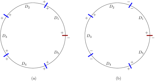
If is even we are in the bipartite case, and we can choose for each , in which case is the Laplacian. We therefore only consider odd , and introduce a single cut at , as was done in [18]. As weight functions we take for , and for we take and , see Figure 5.1(a).
For the operator we recall from (1.12) the compatibility condition on the common boundaries of and , which here says that functions in the domain of should be continuous at each except the cut, where . We recall also from (2.6) the transmission conditions . The outward normal derivative is at the left end-point and at the right end-point, so functions in the domain of should be differentiable at each except the cut, where . In summary, we have
| (5.2) |
This operator is known as the anti-periodic Hill operator or the magnetic Laplace operator on a circle with flux .
The spectrum of consists of eigenvalues , where is positive and odd. Each eigenspace is two dimensional, spanned by and . The partition is -nodal since it is generated by the eigenfunction . The minimal label of the corresponding eigenvalue is and thus , as claimed above.
We now turn to the Dirichlet-to-Neumann operator, for which we use a different valid choice of weights444The two choices of weights are edge equivalent, therefore the Laplacian is identical to ., letting and for all ; see Figure 5.1(b). The condition for the boundary data to be in the subspace defined in (3.1) is , yielding , . For this choice of , the boundary value problem (3.2) becomes
| (5.3) |
with the general solution
where is an arbitrary constant. According to Remark 3.2, we can calculate the Dirichlet-to-Neumann map using any solution to the boundary value problem, so we choose . It follows immediately that
for each , hence the two-sided normal derivative vanishes on , and
| (5.4) |
as expected.
Appendix A Weights, cuts and pair compatibility conditions
In this section we elaborate on some of our constructions and their connection to previous literature. In Section A.1 we discuss the relationship between the strong pair compatibility condition in Definition 1.6, and the weak pair compatibility that appeared in earlier works, such as [16], where it was simply referred to as the pair compatibility condition. In Section A.2 we describe the cutting construction of [18], and explain how it is related to the valid weights introduced in Definition 1.3.


A.1. Weak vs strong pair compatibility conditions
The strong pair compatibility condition (SPCC) was already described in Definition 1.6, which we repeat here for convenience.
Definition A.1.
A two-sided, weakly regular partition is said to satisfy the strong pair compatibility condition (SPCC) if there exists a choice of positive ground states for the Dirichlet Laplacians on such that, for any pair of neighbors , the function defined by
| (A.1) |
is an eigenfunction of the Dirichlet Laplacian on .
Nodal partitions obviously satisfy the SPCC. The same is true of spectral minimal partitions (see [17]), and in Proposition 2.7 we showed that a partition satisfies the SPCC if and only if it is -nodal. A partition satisfying the SPCC is necessarily an equipartition, in the sense that the ground state energy (the smallest eigenvalue of the Dirichlet Laplacian) on each is the same. We denote this common value by .
We next recall the weak pair compatibility condition.
Definition A.2.
A two-sided, weakly regular equipartition is said to satisfy the weak pair compatibility condition (WPCC) if for each pair of neighbors , there exists an eigenfunction of the Dirichlet Laplacian on with eigenvalue and nodal set .
Remark A.3.
It is obvious that SPCC implies WPCC. When is simply connected, a bipartite equipartition satisfying WPCC is nodal, and hence satisfies SPCC, by [16, Theorem 1.3]. If is not simply connected, however, it is possible to find an equipartition (for a Schrödinger operator with potential) that satisfies WPCC but not SPCC, as shown in [16, Section 7].
A.2. Weights and cuts
Assuming throughout that is a two-sided, weakly regular partition, with nodal set , we first decompose the smooth part of into disjoint open curves, labeled , so that . Since is two-sided, each is contained in for some . Without loss of generality we can assume , and we denote these labels by and .
Definition A.4.
A subset is called a valid cut of the partition if there exists a choice of orientations on the subdomains such that if and only if and have the same orientation.
It is sometimes convenient to identity a subset with the corresponding closed subset
| (A.2) |
of . We mention that is a valid cut if is a -homological 1-cycle of (viewed as a cell complex) relative to the boundary . It is immediate that the empty set is a valid cut of if and only if is bipartite.
The maximal cut , for which , is always valid — it corresponds to all subdomains having the same orientation. However, usually one is interested in cuts that are as small as possible. We thus say that a cut is minimal if is connected.
Proposition A.5.
[18, Prop 4.2] There exists a minimal valid cut .
Finally, we describe how valid cuts are related to the valid weights in Definition 1.3. Given a set of valid weights , we obtain a valid cut by declaring that if and only if . That is, the cut set is the union of all along which . More precisely, we have the following.
Proposition A.6.
Valid cuts are in one-to-one correspondence with edge-equivalence classes of valid weights.
Proof.
Given a valid cut, i.e. a choice of orientation for each , we get an induced orientation on each . Choosing an orientation on each smooth component of , we obtain a valid set of weights with the property that if and only if is in the cut set . Changing the orientation on any smooth part of will give a different, but edge equivalent, set of weights (recall Definition 2.4), so we get a map from valid cuts to edge-equivalence classes of valid weights. Conversely, a set of valid weights gives an orientation on each , and hence a valid cut. It is easily seen that edge-equivalent weights generate the same cut. ∎
Remark A.7.
The proof of Proposition A.6 suggests an equivalent way to define valid cuts and weights: a cut is valid if a generic closed path in intersects an even number of times, and a choice of weights is valid if the set defines a valid cut. This alternative definition is not as constructive as Definition 1.3, but it has the advantage of not depending on the manifold structure of , and is thus more convenient for considering partitions on metric graphs.
Remark A.8.
Another way of viewing the constructions in this paper is to introduce Aharonov–Bohm operators, as in [18]. Given a set of weights that generates a minimal valid cut, the corresponding is equivalent to a certain Aharonov–Bohm operator, with Aharonov–Bohm solenoids with flux placed at the singular points of for which is odd (recall Definition 1.2).
Appendix B Explicit construction of the canonical solution to (3.2)
In this section we give an alternate, more explicit proof of the second claim in Theorem 3.1, regarding the existence of a “canonical solution” such that and solves (3.2) for each . To do this we write the condition as a finite system of linear equations and then, by analyzing the corresponding matrix, prove that a solution always exists.
Fix . For each , the general solution of (3.2) is given by
| (B.1) |
for some . Since , we know from (3.5) that the two-sided normal derivative is a function in , and is given by on . This will be an element of the subspace if and only if
| (B.2) |
for each . Since each point in the smooth part of is contained in precisely one other , we can rewrite this integral as
| (B.3) | ||||
where we have denoted for convenience. Let us introduce the notations
It follows from (2.8) that on , and so for all . We similarly get
We then define
| (B.4) |
so the equation (B.3) becomes
| (B.5) |
We write the resulting system of equations in matrix form as
| (B.6) |
and observe that the vector lies in the kernel of the matrix .
Without loss of generality, we can label the domains in the partition inductively so that is a neighbor of at least one of , with arbitrary. For the numbers , this means that
| (B.7) |
Lemma B.1.
Proof.
Consider the quadratic form corresponding to the matrix above, where . From (B.5) we find that the quadratic form can be written as
Since for all , we see that (and hence ) is non-negative. It remains to identify the kernel. Assume that for some . Then, reading from the top line above, we conclude that since . Inserting , we conclude from the next row that since . Continuing in this manner, we conclude that . This means that the kernel of is spanned by the vector . ∎
References
- [1] W. Arendt and A. F. M. ter Elst. The Dirichlet-to-Neumann operator on rough domains. J. Differential Equations, 251(8):2100–2124, 2011.
- [2] W. Arendt, A. F. M. ter Elst, J. B. Kennedy, and M. Sauter. The Dirichlet-to-Neumann operator via hidden compactness. J. Funct. Anal., 266(3):1757–1786, 2014.
- [3] Wolfgang Arendt and Rafe Mazzeo. Spectral properties of the Dirichlet-to-Neumann operator on Lipschitz domains. Ulmer Seminare, 12:28–38, 2007.
- [4] Wolfgang Arendt and Rafe Mazzeo. Friedlander’s eigenvalue inequalities and the Dirichlet-to-Neumann semigroup. Commun. Pure Appl. Anal., 11(6):2201–2212, 2012.
- [5] Ram Band, Graham Cox, and Sebastian Egger. Defining the spectral position of a Neumann domain. arXiv:2009.14564, 2021.
- [6] J. Behrndt and A. F. M. ter Elst. Dirichlet-to-Neumann maps on bounded Lipschitz domains. J. Differential Equations, 259(11):5903–5926, 2015.
- [7] Gregory Berkolaiko, Yaiza Canzani, Graham Cox, and Jeremy L. Marzuola. Spectral minimal partitions, nodal deficiency and the Dirichlet-to-Neumann map: the generic case. arXiv:2201.00773, 2022.
- [8] Gregory Berkolaiko, Graham Cox, and Jeremy L. Marzuola. Nodal deficiency, spectral flow, and the Dirichlet-to-Neumann map. Lett. Math. Phys., 109(7):1611–1623, 2019.
- [9] Gregory Berkolaiko, Peter Kuchment, and Uzy Smilansky. Critical partitions and nodal deficiency of billiard eigenfunctions. Geom. Funct. Anal., 22(6):1517–1540, 2012.
- [10] Lipman Bers. Local behavior of solutions of general linear elliptic equations. Comm. Pure Appl. Math., 8:473–496, 1955.
- [11] Virginie Bonnaillie-Noël and Bernard Helffer. Nodal and spectral minimal partitions—the state of the art in 2016. In Shape optimization and spectral theory, pages 353–397. De Gruyter Open, Warsaw, 2017.
- [12] Graham Cox, Christopher K.R.T. Jones, and Jeremy L. Marzuola. Manifold decompositions and indices of Schrödinger operators. Indiana Univ. Math. J., 66:1573–1602, 2017.
- [13] Monique Dauge. Elliptic boundary value problems on corner domains, volume 1341 of Lecture Notes in Mathematics. Springer-Verlag, Berlin, 1988. Smoothness and asymptotics of solutions.
- [14] Leonid Friedlander. Some inequalities between Dirichlet and Neumann eigenvalues. Arch. Rational Mech. Anal., 116(2):153–160, 1991.
- [15] Pierre Grisvard. Elliptic problems in nonsmooth domains, volume 69 of Classics in Applied Mathematics. Society for Industrial and Applied Mathematics (SIAM), Philadelphia, PA, 2011.
- [16] B. Helffer and T. Hoffmann-Ostenhof. Converse spectral problems for nodal domains. Mosc. Math. J., 7(1):67–84, 167, 2007.
- [17] B. Helffer, T. Hoffmann-Ostenhof, and S. Terracini. Nodal domains and spectral minimal partitions. Ann. Inst. H. Poincaré Anal. Non Linéaire, 26(1):101–138, 2009.
- [18] Bernard Helffer and Mikael Persson Sundqvist. Spectral flow for pair compatible equipartitions. Communications in Partial Differential Equations, pages 1–28, 2021.
- [19] William McLean. Strongly elliptic systems and boundary integral equations. Cambridge University Press, Cambridge, 2000.
- [20] Konrad Schmüdgen. Unbounded self-adjoint operators on Hilbert space, volume 265 of Graduate Texts in Mathematics. Springer, Dordrecht, 2012.