Improving the Quality Control of Seismic Data through Active Learning

Abstract

In image denoising problems, the increasing density of available images makes an exhaustive visual inspection impossible and therefore automated methods based on machine-learning must be deployed for this purpose. This is particulary the case in seismic signal processing. Engineers/geophysicists have to deal with millions of seismic time series. Finding the sub-surface properties useful for the oil industry may take up to a year and is very costly in terms of computing/human resources. In particular, the data must go through different steps of noise attenuation. Each denoise step is then ideally followed by a quality control (QC) stage performed by means of human expertise. To learn a quality control classifier in a supervised manner, labeled training data must be available, but collecting the labels from human experts is extremely time-consuming. We therefore propose a novel active learning methodology to sequentially select the most relevant data, which are then given back to a human expert for labeling. Beyond the application in geophysics, the technique we promote in this paper, based on estimates of the local error and its uncertainty, is generic. Its performance is supported by strong empirical evidence, as illustrated by the numerical experiments presented in this article, where it is compared to alternative active learning strategies both on synthetic and real seismic datasets.

1 Introduction

Our goal is to perform noise detection, which are very structured and contain information on the composition of the subsurface. To this end, we present a new active learning algorithm that can perform this task after being manually trained by an expert, with minimal training time. The "images" on which we want to perform noise detection are the concatenation of seismic times series into a coherent image. Each time series is the measure by a sensor of the response of the subsurface to an artificial sound source at a particular geographical point. They are called "shot point gather" in geophysics research field. Those images are then used within an inverse problem to obtain a 3D "images" of the subsurface and derived its properties (porosity, velocity…) (barclay2008). Providing accurate properties of the subsurface, for instance below the oceans (yilmaz1), requires seismic data, what we denote images in our approach, to go through a large number of signal processing steps, so that they can be efficiently used within the inverse problem. Among these steps, tasks dedicated to the removal of various types of noise are particularly important and subject to errors due to their inherent complexity. They are handled by various specific algorithms that are cascaded within workflows and all contain user-defined parameters tuned by humans (called processing geophysicists), such that the quality of the results is controlled with respect to these parameters in order to minimize the residual noise. These quality controls (QCs) are often done manually (castelao2021), which is demanding due to the large volume of the seismic data (terabytes of data). In this paper, the problem of automatically detecting residual noise in seismic processed images in our case with the objective of controlling the quality of the denoised images, is considered from a machine-learning perspective. Specifically, we investigate how to apply machine-learning techniques to train a classifier detecting the presence of noise or residual noise. This is undeniably a Big Data issue in every sense of the term, insofar as billions of images are currently available for each seismic survey. A Seismic image have dimensions of at least $500\times 2500$ pixels. Whereas the problem of learning a predictive rule to detect the presence of possible noise, using a preprocessed seismic image as input, can be naturally cast as a multi-class classification problem, the performance that can be achieved is conditioned by the availability of a sufficiently large number of labeled data containing both well and poorly denoised images. Obtaining a large number of labeled images is extremely difficult and costly.

The goal of this paper is to present a new method to build a classifier for noise detection that uses as little training data as possible. We present a new active learning technique, which allows us to find the most relevant training images in order to improve our classifier. By doing so, we iteratively improve the classifier by enhancing our training set with the most relevant data. As a consequence, the classifier trained on this adapted dataset has very good performance, even though it was trained on little data. Finally, this procedure will allow us to continue improving our noise detection algorithm as new data is obtained.

This paper is organized as follows: We start by first presenting the very specific structure of the seismic images and then give an overview of the machine learning modeling of the problem. In a second step, we present our active learning method and its algorithms. Finally, we test our method on several datasets: one proprietary dataset of seismic images and one classical machine learning dataset that is well suited for this kind of classification problem.

2 Seismic data and machine learning background

In the seismic experiments considered here, a sound source is towed by a boat and generates waves that will propagate in the subsurface and be reflected back to the surface when the waves encounter discontinuities in the subsurface. These waves are then recorded by sensors regularly distributed along cables located near the surface of the water that are also towed by a boat. Those time series then go through a complicated processing sequence (mari1997) to obtain properties of the subsurface (yilmaz1).

In the seismic image shown in Figure 1, each column represents the amplitude measured by a sensor over time and can be read from top to bottom (increasing recording time), with grey scale representing the amplitude of the reflected waves. Two adjacent columns correspond to two adjacent sensors along a cable measuring a very similar seismic response. This leads to a coherent and colored (with respect to the amplitude) seismic image, as displayed in Figure 1.

The blue curve on this image represents the wave reflection of the sea floor. These images are usually made up of $10^{6}$ pixels. Finally, a seismic survey usually covers $10,000$km² and contains millions of such images, i.e.  billions of time series and can easily require $40$ Tera octets of storage capacity.

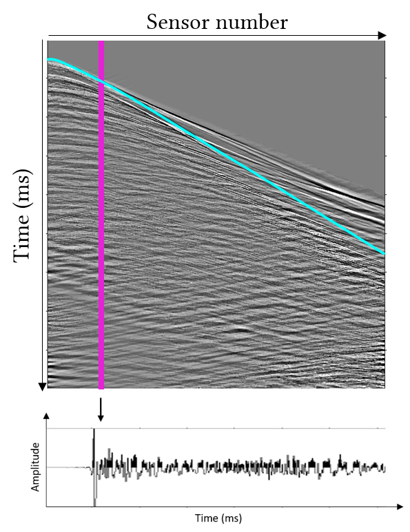
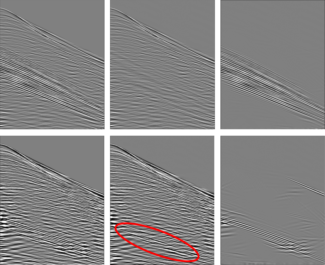
Figure 1: On the left : top, A seismic image, composed of many seismic time series, corresponding to the recordings of many sensors at one particular location. Bottom: One seismic time series, i.e.  , one sensor. On the right : two examples (top versus bottom) of an original image (left), its denoised version (center) and the corresponding extracted noise (right): the denoise process on top is efficient, while that on the bottom exhibits some residual noise (red circled area)

2.1 Seismic processing

Seismic processing consists of finding accurate properties of the subsurface from the raw seismic time series records (yilmaz1; taner1979). However, while the recorded images contain signal (i.e.  , desired seismic events), they will also contain noise, which may compromise the inverse problem to find the properties of the subsurface. In practice, the seismic processing sequence is made up of tens of numerical processing steps applied to the data to prepare it for the inverse problem that will lead to certain properties of the subsurface usable for the interpretation. In the following, we will only focus on the process of noise removal. Before and after examples are displayed in Figure 1. The cleaning process is heavy in human and computer time and should be performed with maximum care. The issue of the processing sequence is that if some noise remains in the data at a particular processing step, or if a processing step creates an issue with the data, it can affect adjacent time series during the processing flow and lead to an unrealistic representation of the subsurface. Should an issue on the data be detected a posteriori, the entire process will have to be rerun from scratch, entailing both a considerable schedule delay and extra machine and human cost.

2.2 Machine learning and noise detection

Following the statistical learning paradigm (hastie2001), generic seismic data, i.e.  shot gather image in our case, is viewed as a random pair $(X,Y)$ of input and output, with joint unknown distribution $\bbP_{(X,Y)}$. The input $X\in\mathbb{R}^{d}$ corresponds to the seismic image (i.e.  the concatenation of times series) and the output $Y\in\{0,1\}$ to a quality label. It equals $0$ if the image passes the quality control check, i.e.  if there is no residual noise in $X$, and equals $1$ as soon as the presence of residual noise is suspected. In that case, the image should be evaluated by an expert. The dataset, indexed by $\I\subset\bbN$ with cardinal $|\I|$, is modeled as a collection $(X_{i},Y_{i})_{i\in\mathcal{I}}$ of independent copies of the random vector $(X,Y)$. The index set $\mathcal{I}$ can be decomposed as $\mathcal{I}=\mathcal{L}\cup\mathcal{T}\cup\mathcal{U}$, where $\mathcal{L}$ and $\mathcal{T}$ respectively identify the learning set and the test set, both made of labeled data, while $\U$ designates the unlabeled observations.

The goal in machine learning is to find a function $g:\mathbb{R}^{d}\to\{0,1\}$, called a classifier, that accurately predicts $Y$ given $X$. It is generally constructed from the training dataset to be optimal in some sense. Then, its performance is evaluated through its risk, defined as

$$\mathcal{R}_{g}:=\mathbb{E}(\ell(Y,g(X)))$$

where $\ell(y,y^{\prime})\{0,1\}\times\{0,1\}\to\{0,1\}=1_{y\neq y^{\prime}}$. In practice, since it relies on the unknown distribution $\mathbb{P}_{(X,Y)}$, it is replaced by its empirical version, computed from the test set:

$$\widehat{\mathcal{R}}_{g}:=\frac{1}{|\mathcal{T}|}\sum_{i\in\mathcal{T}}\ell(Y_{i},g(X_{i})).$$

In order to improve the classifier, the training set can be extended by labeling some elements of $\U$ and adding them to $\mathcal{L}$. They are usually picked at random, uniformly in $\mathcal{U}$. Proceeding so guarantees convergence towards an optimal classifier as the number of labeled data tends to infinity. Nevertheless, it may take a lot of labeled data to reach an efficient, satisfactory classifier.

In the present situation, labeling seismic data is very costly. Thus, improving the speed of convergence of the classifier towards its equilibrium is paramount: the amount of labeled data needed to get a sufficient result should be as small as possible. To acheve this, the active learning paradigm proposes selecting the most relevant data in the unlabeled set, instead of picking these new observations purely at random.

3 Our method: local risk-based active learning strategy

We present our solution to the noise detection problem, which includes efficiently building a classifier thanks to a new active learning strategy.

3.1 Optimal classifier: minimizing the estimated local risk

In order to implement an active learning scheme, the training set needs to be enhanced with the data that has maximum influence on risk minimization. We adopt an approach based on the local risk function, defined for a classifier $g$ and a loss function $\ell$ as the mapping:

$$x\in\bbR^{d}\mapsto R_{g}(x):=\mathbb{E}(\ell(Y,g(X))\mid X=x).$$

It is related to the risk $\mathcal{R}_{g}$ through the chain rule

$$\mathcal{R}_{g}=\mathbb{E}(\ell(Y,g(X)))=\mathbb{E}(\mathbb{E}(\ell(Y,g(X))\mid X))=\mathbb{E}(R_{g}(X)).$$

To this end, the unlabeled data that maximizes the local risk function would be selected and experts would be asked to label it. Then, the corresponding input-output couple would be added to the training set, with index

$$i_{\ast}:=\underset{{i\in\mathcal{U}}}{\mathrm{argmax}}\ R_{g}(X_{i}).$$

Intuitively, thinking of the graph of the local risk function as a surface in $\mathbb{R}^{d}\times[0,1]$, this amounts to selecting its high peaks and setting them to $0$ in the next update of the classifier. This approach is expected to work under the condition that, when adding a point to the training set, the local risk function does not change drastically, and new peaks do not appear (thereby avoiding a whack-a-mole configuration). This should be the case for local classifiers such as $k$-nearest-neighbors or random forests. This approach is not expected to perform well with non-local classifiers, such as logistic regression. Choosing a point according to the $L^{\infty}$ norm to minimize the $L^{1}$ norm may be surprising at first glance. The distribution $\mathbb{P}_{X}$ is unknown. If one approximates $\bbP_{X}$ by the empirical distribution of the $X_{i}$’s for $i\in\U$ $\widehat{\bbP_{X}}=\frac{1}{|\U|}\sum_{i\in\U}\delta_{X_{i}},$ then the risk of a classifier $g$ can be written as

$$\mathcal{R}_{g}\approx\frac{1}{|\U|}\sum_{i\in\U}R_{h}(x_{i}).$$

With this representation, the most relevant data to label is the one maximizing the local risk.

Unfortunately, this approach cannot be performed exactly, as it relies on the unknown distribution $\mathbb{P}_{(X,Y)}$. The vector $(R_{g}(X_{i}))_{i\in\U}$ of the local risk function taken at each unlabeled data point is replaced by an estimator $(\widehat{R_{g}(X_{i})})_{i\in\U}$. Incidentally, $i_{\ast}$ is redefined as

$$i_{\ast}:=\underset{{i\in\mathcal{U}}}{\mathrm{argmax}}\text{ }\widehat{R_{g}(X_{i})}.$$ (1)

When several indices reach this maximum, $i_{\ast}$ is picked at random, uniformly among them. A plethora of estimators could be chosen to assess the local risk function. We opted for the Nadaraya-Watson (also called local-constant) estimator, for both its non-parametric and local qualities; using a local estimator for a local classifier seems sensible. Given a window parameter $h\in\bbR^{+}$ and a kernel function $K_{h}$ (typically the standard Gaussian kernel $(x,x^{\prime})\in\bbR^{d}\times\bbR^{d}\mapsto e^{-\|x-x^{\prime}\|^{2}/h}$), this estimator of the local risk function at point $x\in\bbR^{d}$ is defined as

$$\widehat{R_{g}(x)}:=\sum_{i\in\L}\ell(Y_{i},g(X_{i}))\,\dfrac{K_{h}(x,X_{i})}{\sum\limits_{j\in\L}K_{h}(x,X_{j})}.$$

In the sequel, when necessary, its dependence on $h$ and $\L$ shall be made explicit by writing $\widehat{R_{g}}(x;h,\L)$.

3.2 Batch approach and survey schemes

The seismic data experts who will label new observations, are humans (geophysicists). From a practical point of view, it is sub-optimal to occasionally solicit them to label a single image. Taking this into account, our procedure is readily adapted to the case where batches of $K\in\bbN$ images are added to the training set at each update of the classifier. After consulting with the geophysics experts we work with, it was decided to set $K\approx 20$ (this task is completed in about $15$ minutes).

Alternately, the selection process could be made random to favor the exploration of the input space. In the vein of CBCP19 or beygelzimer2009, a conditional Poisson sampling design could be used to that effect. The general idea is to give priority to the unlabeled data with high estimated local risk, but still allow the others to be picked once in a while. Precisely, each candidate $i\in\U$ is given a sampling weight $\pi_{i}\in[0,1]$, named inclusion probability, such that $\sum_{i\in\U}\pi_{i}=K$. Then, it is selected independently according to the result of a Bernoulli trial with probability $\pi_{i}$. The procedure is repeated until exactly $K$ elements of $\U$ are selected (LABEL:alg:survey). The inclusion probabilities are taken proportional to the estimated local risk (possibly augmented by its variance):

$$\forall\,i\in\U,\quad\pi_{i}:=K\,\dfrac{\widehat{R_{g}(X_{i})}}{\sum\limits_{j\in\U}\widehat{R_{g}(X_{j})}}.$$ (2)

It can happen that some number $K_{0}$ of them exceed $1$. In that case, the corresponding data are automatically chosen and the process is restarted with the remaining data, using $K-K_{0}$ instead of $K$ in (2).

4 Algorithms

In this section, we give all the algorithms to precisely implement our methods, in the same order as presented above. We start with the empirical risk minimization, where the parameter $h$ in the kernel is computed thanks to the classical leave-one-out cross-validation method.

[]