EMPRESS. VII.
Ionizing Spectrum Shapes of Extremely Metal-Poor Galaxies:
Uncovering the Origins of Strong Heii and the Impact on Cosmic Reionization

Abstract

Strong high-ionization lines such as He ii of young galaxies are puzzling at high and low redshift. Although recent studies suggest the existence of non-thermal sources, whether their ionizing spectra can consistently explain multiple major emission lines remains a question. Here we derive the general shapes of the ionizing spectra for three local extremely metal-poor galaxies (EMPGs) that show strong He ii$\lambda$4686. We parameterize the ionizing spectra composed of a blackbody and power-law radiation mimicking various stellar and non-thermal sources. We use photoionization models for nebulae, and determine seven parameters of the ionizing spectra and nebulae by Markov Chain Monte Carlo methods, carefully avoiding systematics of abundance ratios. We obtain the general shapes of ionizing spectra explaining $\sim 10$ major emission lines within observational errors with smooth connections from observed X-ray and optical continua. We find that an ionizing spectrum of one EMPG has a blackbody-dominated shape, while the others have convex downward shapes at $>13.6$ eV, which indicate a diversity of the ionizing spectrum shapes. We confirm that the convex downward shapes are fundamentally different from ordinary stellar spectrum shapes, and that the spectrum shapes of these galaxies are generally explained by the combination of the stellar and ultra-luminous X-ray sources. Comparisons with stellar synthesis models suggest that the diversity of the spectrum shapes arises from differences in the stellar age. If galaxies at $z\gtrsim 6$ are similar to the EMPGs, high energy ($>54.4$ eV) photons of the non-stellar sources negligibly contribute to cosmic reionization due to relatively weak radiation.

1 Introduction

Understanding the epoch of reionization (EoR) is one of the most important goals for astronomy today. Many studies have suggested that galaxies are the dominant sources of ionizing photons at EoR (e.g., Wise et al., 2014; Madau & Haardt, 2015; Stanway et al., 2016). From the hydrodynamical simulations, high-redshift young galaxies at the early formation phase are expected to have low metallicities, low stellar masses, and high specific star formation rates (e.g., Wise et al., 2012). High-redshift galaxies are studied with various large telescopes including the Hubble Space Telescope (HST) (e.g., Bouwens et al., 2015; Livermore et al., 2017; Atek et al., 2018; Oesch et al., 2018; Harikane et al., 2016; Kikuchihara et al., 2020). Although there are spectroscopic studies for very bright or lensed galaxies at high redshifts (e.g., Shibuya et al., 2018; Mainali et al., 2018; Stark et al., 2015), dwarf galaxies at high-redshift are too faint to be detected with current observational instruments. For example, even with upcoming James Webb Space Telescope (JWST), we can detect H$\alpha$ for galaxies with stellar mass below $10^{6}~{}M_{\odot}$ only at $z\lesssim 2$ without gravitational lensing (Isobe et al., 2021a)

Owing to the observational difficulties, many studies use local dwarf galaxies as analogs of high-redshift young dwarf galaxies (e.g., Berg et al., 2019). Among the local dwarf galaxies, local extremely metal-poor galaxies (EMPGs) are recently gaining attention (e.g., Izotov & Thuan, 1998; Thuan & Izotov, 2005; Sánchez Almeida et al., 2016; Kojima et al., 2020). EMPGs are defined as galaxies with metallicity below $10\%$ solar metallicity $Z_{\odot}$. So far, EMPGs with metallicities down to $1.6\%~{}Z_{\odot}$ have been identified using data obtained with Subaru/Hyper Suprime Cam (HSC) (Kojima et al., 2020). Local EMPGs have low masses and high specific star-formation rates (sSFRs), both of which are comparable to those of high-redshift young galaxies (e.g., Wise et al., 2012). Local EMPGs are therefore regarded as local analogs of high-redshift young galaxies.

The importance of relationships between local EMPGs and high-redshift galaxies is further emphasized because very strong high-ionization nebular emission lines (i.e., He ii, C iii], C iv) are detected from local EMPGs (Berg et al., 2019; Senchyna et al., 2017; Guseva et al., 2000; Shirazi & Brinchmann, 2012; Kojima et al., 2021) and high-redshift galaxies (Stark et al., 2015; Schmidt et al., 2017; Laporte et al., 2017; Mainali et al., 2018). Most of the EMPGs have detections of optical recombination lines He ii$\lambda$4686 that need high energy ionizing photons ($>54.4~{}{\rm eV}$) (López-Sánchez & Esteban, 2010; Shirazi & Brinchmann, 2012; Senchyna et al., 2017). A statistical study of local galaxies shows that fluxes of He ii $\lambda 4686$ increase as the metallicities decrease (e.g., Schaerer et al., 2019). These results indicate the presence of hard ionizing sources in the metal-poor environments.

The origin of strong He ii emission line is still under debate. Xiao et al. (2018) examine contributions from stellar radiation using the photoionization code cloudy (Ferland et al., 2013) and the Binary Population and Spectral Synthesis (BPASS) code (Stanway et al., 2016; Eldridge et al., 2017). BPASS binary models incorporate contributions from hard radiation from Wolf-Rayet stars and stripped binary stars. However, a line ratio He ii$\lambda$4686/H$\beta$ predicted in Xiao et al. (2018) falls short of the observed value by more than 0.5 dex, suggesting that stars are not major contributors to the He ii ionizing photons. Addition of extra stars (e.g., metal-poor, very massive, or Wolf-Rayet stars) could boost the He ii ionizing photons, but several studies suggest that these stars cannot fully account for the observed strength of He ii in EMPGs (e.g., Kehrig et al., 2018; Olivier et al., 2021). Pérez-Montero et al. (2020) suggest that ordinary stellar synthesis models with non-zero ionizing photon escape fraction can explain He ii$\lambda$4686/H$\beta$, but their models require very high escape fraction values ($\sim 70\%$) that are not compatible with the typical values reported for $z\lesssim 3$ galaxies (e.g., Izotov et al., 2021c; Rutkowski et al., 2016; Alavi et al., 2020; Steidel et al., 2018; Saxena et al., 2022).

Non-thermal ionizing sources have been proposed to explain the strong nebular He ii from EMPGs. Active galactic nuclei (AGNs) are one of the candidates of non-thermal emission sources (e.g., Berg et al., 2018; Plat et al., 2019). Berg et al. (2018) find that AGN models can reproduce observed He ii$\lambda$1640, while that other emission lines, such as C iv$\lambda$$\lambda$1548,1551 and C iii]$\lambda$1909 cannot be reproduced simultaneously. However, their AGN models does not consider metal-poor ($<0.25$ $Z_{\odot}$) AGNs. Shocks are another candidates for the ionizing sources of He ii (e.g., Thuan et al., 2005; Isobe et al., 2021b; Berg et al., 2018; Plat et al., 2019). Berg et al. (2018) also examine contributions from radiative shocks using radiative shock models of Allen et al. (2008). The calculations with the radiative shock models also suggest that radiative shocks cannot explain the strong He ii$\lambda$1640 emission for a given intensity of other emission lines such as C iv$\lambda$$\lambda$1548,1551 and C iii]$\lambda$1909 (see also Izotov et al. 2021a).

Alternatively, other hard radiation sources are also proposed. Schaerer et al. (2019) show that X-ray luminosities have a positive correlation with line ratios He ii$\lambda$4686/H$\beta$ with X-ray binary population models, indicating the contributions of the He ii ionizing photons from high mass X-ray binaries (HMXBs). Lebouteiller et al. (2017) demonstrate that HMXBs can be the sources of He ii ionizing photons in well-studied EMPG I Zw 18 through detailed modeling of radiation fields and interstellar mediums. Kehrig et al. (2021) argue that the ultra-luminous X-ray source (ULX) in I Zw 18 cannot fully account for all of He ii ionizing photons. However, new integral field spectroscopic observations of I Zw 18 suggest that the ULX still remains the possibility (see Rickards Vaught et al., 2021). Moreover, while Senchyna et al. (2020) argue that HMXBs cannot be the main contributors of He ii in EMPGs through the photoionization models representing HXMB spectra by simple multi-color disk models, Simmonds et al. (2021) examine the photoionization models using several detailed spectrum models for HMXBs/ULXs and find that some of the models can reproduce He ii$\lambda$4686/H$\beta$ and other line ratios such as [O iii]$\lambda$$\lambda$4959,5007/H$\beta$ and [O iii]$\lambda$$\lambda$4959,5007/[O ii]$\lambda$3727. The studies of Schaerer et al. (2019), Simmonds et al. (2021), and Lebouteiller et al. (2017) claim that HMXB/ULX can explain strong He ii emission lines (cf. Saxena et al. 2020 and Senchyna et al. 2020), but whether a simple physical model can explain all the emission lines from a galaxy in a self-consistent manner remains uncertain. There are also attempts to explain emission lines from EMPGs by non-uniform inter-stellar medium (ISM) (e.g., Berg et al., 2021; Izotov et al., 2021a; Ramambason et al., 2020). For example, Ramambason et al. (2020) show that ordinary stellar population synthesis models can reproduce high-ionization emission lines [O iii]$\lambda$$\lambda$4959,5007 simultaneously with low-ionization emission lines [O ii]$\lambda$3727 by introducing so-called “two-zone” models.

Variations of models presented by these previous studies raise difficulties in reproducing strong He ii emission line fluxes for given low-ionization line fluxes. Instead, we aim to determine the self-consistent general spectrum shape by a parametric method. By obtaining the general spectrum shapes first, we can infer the possibility of countless ionization sources without running costly calculations using photoionization code each time. Moreover, we expect to uncover the spectral features that were not previously mentioned.

In this work, we search for the self-consistent spectrum shapes that can reproduce observed emission line fluxes of three EMPGs. Similar work such as Olivier et al. (2021) (hereafter, O21) uses a blackbody and BPASS models to search for the spectrum shape. Another similar study uses combinations of BPASS models and ULX models as ionizing spectra (Simmonds et al., 2021). With the minimum assumptions, we construct generalized spectral models that cover spectrum shapes examined in O21 and Simmonds et al. (2021). We use a generalized spectrum as an ionizing spectrum in a uniform ISM to compute emission line fluxes using photoionization code cloudy. We then search for the self-consistent spectrum shapes using Markov Chain Monte Carlo (MCMC) method.

Our sample and methodology are described in Section 2. We present our results for the general spectrum shapes and reproduction of emission lines in Section 3. In Section 4, we evaluate several candidates for the hard radiation sources using the general spectrum shape. We also examine the contributions of the hard radiation sources to cosmic reionization. In Section 5, we summarize our main results. Throughout this paper, magnitudes are in the AB system, and we assume a standard $\Lambda$ CDM cosmology with parameters of ($\Omega_{\rm m}$, $\Omega_{\rm\Lambda}$, $H_{0}$) = (0.3, 0.7, 70 km s^-1${\rm Mpc}^{-1}$) and the solar metallicity scale of Asplund et al. (2009), where $12$+$\log({\rm O/H})$=8.69.

Table 1: Sample Properties

Name of the Galaxy	$z$	$i$	$\log$($M_{\star}$)	$\log$(SFR)	$Z$	$F$(H$\beta$)	$\textrm{EW}_{0}$(H$\beta$)	$L_{{\rm X,}0.5-10~{}{\rm keV}}$	References
		(mag)	($M_{\odot}$)	($M_{\odot}$ yr-1)	($Z_{\odot}$)	($10^{-14}~{}$erg s-1 cm-2)	(Å)	($10^{39}$ erg s-1)
	(1)	(2)	(3)	(4)	(5)	(6)	(7)	(8)	(9)
J1631+4426	$0.031$	$22.5$	$5.9$	$-1.28$	$0.016$	$0.13$	$123.5$	$\cdots$	(a)
J104457	$0.013$	$18.7$	$6.8$	$-0.85$	$0.058$	$0.95$	$\cdots$	$\cdots$	(b), (c)
I Zw 18 NW	0.002	$20.1$	$5.5$	$-2.70$	$0.030$	$3.19$	$81.2$	$1.4-1.6$	(d), (e), (f), (g)

Note. — (1): Redshift. (2): $i$-band magnitude. The magnitudes are the cmodel magnitudes of Subaru/HSC (SDSS) for J1631+4426 (J104457 and I Zw 18 NW). (3): Stellar mass. (4): Star-formation rate (SFR). The SFR of I Zw 18 NW is derived from the H$\alpha$ flux in the same manner as Isobe et al. (2021b). (5): Gas-phase Metallicity derived by the direct $T_{\rm e}$ method. (6): H$\beta$ flux. (7): Rest-frame equivalent width of an H$\beta$ emission line. (8): X-ray luminosity at $0.5-10.0$ keV obtained by ${\it Chandra}$ X-ray observations. (9): References for values in the columns $(1)-(8)$: (a) Kojima et al. (2020), (b) B21, (c) SDSS DR2 (Abazajian et al., 2004), (d) SDSS DR6 (Adelman-McCarthy et al., 2008), (e) TI05, (f) Lebouteiller et al. (2017), (g) Thuan et al. (2004)

2 Sample and Methods

2.1 Sample

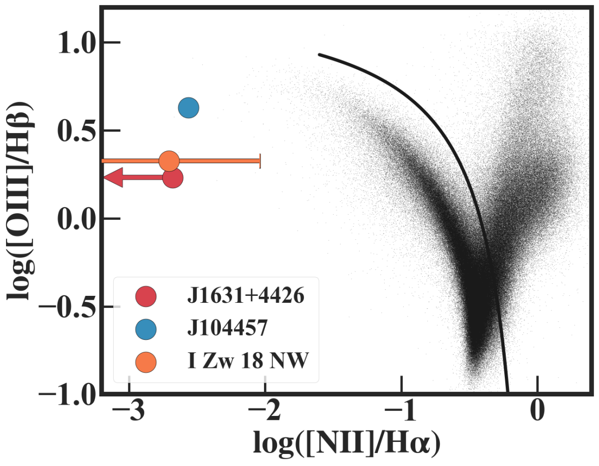
We investigate general ionizing spectrum shapes for a sample of three galaxies, J1631+4426, J104457, and I Zw 18 NW, whose properties are summarized in Table 1. All three galaxies are extremely metal-poor ($Z<10\%~{}Z_{\odot}$), nearby ($z\sim 0$), and low-mass ($\lesssim 10^{6}M_{\odot}$) galaxies. J1631+4426 is the most metal-poor galaxy detected, with $Z=1.6\%~{}Z_{\odot}$ (Kojima et al., 2021, hereafter, K21). Thus, J1631+4426 is a good test-bed for investigating the nature of EMPGs. J104457 is a metal-poor galaxy, whose optical spectrum has been studied previously and shown that BPASS models alone cannot explain high-energy ionization lines (Berg et al., 2021, hereafter, B21). Olivier et al. (2021) have also studied J104457 and have shown that the combination of a blackbody and BPASS model can explain multi-level emission lines of J104457. Therefore, we can compare our results to those of Olivier et al. (2021). I Zw 18 NW is one of the most well-known EMPG that has optical and X-ray data (Thuan & Izotov, 2005, hereafter, TI05). This allows us to check the consistency between the ionizing spectrum shapes beyond 54.4 eV and X-ray luminosity data for I Zw 18 NW. All three galaxies in our sample have optical spectroscopic data available. In Figure 1, we present the locations of all three galaxies on a diagram of [N ii]$\lambda$6583/H$\alpha$ and [O iii]$\lambda$5007/H$\beta$ emission line ratios, so-called the Baldwin-Philips-Terlevich diagram (BPT diagram; Baldwin et al., 1981). The black dots represent the emission line ratios of $z\sim 0$ star forming galaxies (SFGs) and AGNs from the Sloan Digital Sky Survey (SDSS) Data Release 7 (DR7) (Abazajian et al., 2009). [N ii]$\lambda$6583/H$\alpha$ and [O iii]$\lambda$5007/H$\beta$ emission line ratios for all three galaxies can be explained by only stellar radiation (Kauffmann et al., 2003). However, because Kewley et al. (2013) suggest that metal-poor gas heated by AGN can produce emission line ratio values that fall on the SFG region, we cannot conclude the contributions from AGNs from this classification.

Figure 1: Our three galaxies on the BPT diagram. The red, blue, and orange dots represent the emission line ratios of J1631+4426, J104457, and I Zw 18 NW, respectively. The bars represent errors of the emission line ratios. The red arrow indicates an upper limit with $1\sigma$ level for [N ii]$\lambda$6583/H$\alpha$ of J1631+4426. The black dots represent $z\sim 0$ SFGs and AGNs derived from the emission line catalog of SDSS DR7. The solid curve depicts the maximum photoionization models that can be reproduced solely by stellar radiation (Kauffmann et al., 2003). The region left (right) to the solid curve is the SFG (AGN and composite) region.

In this work, we use observed optical emission lines from hydrogen, helium, oxygen, and sulfur ions to determine the best-fit model parameters. The optical emission lines and their flux ratios are listed in Table 2. We avoid using H$\alpha$ for the fitting of J1631+4426 because the reported H$\alpha$ flux is not consistent with the Balmer decrements. We also avoid using H$\alpha$ for the fitting of I Zw 18 NW because the value of H$\alpha$ flux has been obtained using a different spectrometer from the one used to obtain the fluxes of the other lines. We use line ratios between sulfur doublets [S ii]$\lambda$6316/$\lambda$6731 instead of line ratios between sulfur and hydrogen to minimize effects from the uncertainty of sulfur’s abundance ratio to oxygen. Another reason to use [S ii]$\lambda$6316/$\lambda$6731 is that this line ratio is sensitive to the gas density in H ii regions (Osterbrock & Ferland, 2006). We avoid including emission line fluxes from other elements to minimize systematics of abundance ratios. We note that He ii$\lambda$4686 lines of J1631+4426 and J104457 are narrow and have no broad-line features (Kojima et al., 2021; Berg et al., 2021). There is a report of a Wolf-Rayet bump centered at 4645 Å for I Zw 18 NW, but no underlying broad component is detected for He ii$\lambda$4686 (Legrand et al., 1997). Therefore, we treat He ii$\lambda$4686 lines of our three galaxies as the nebular origin. All the line ratios in Table 2 use the dust-corrected fluxes.

Table 2: Fluxes and Flux ratios

Ion	J1631+4426	J104457	I Zw 18 NW
$F_{\lambda}/F_{{\rm H\beta}}$
[O ii]$\lambda$$\lambda$3727,3729	50.12$\pm$2.66	26.37$\pm$0.27	37.66$\pm$0.61
He i$\lambda$4026	$\cdots$	1.72$\pm$0.03	1.03$\pm$0.09
H$\delta$	27.53$\pm$0.65	25.59$\pm$0.42	26.52$\pm$0.42
H$\gamma$	46.88$\pm$0.50	46.55$\pm$0.67	47.53$\pm$0.71
[O iii]$\lambda$4363	8.18$\pm$0.48	13.51$\pm$0.21	6.74$\pm$0.14
He i$\lambda$4471	$\cdots$	3.97$\pm$0.09	2.76$\pm$0.08
He ii$\lambda$4686	2.32$\pm$0.38	1.80$\pm$0.04	3.44$\pm$0.09
H$\beta$	100.00$\pm$0.37	100.0$\pm$1.4	100.00$\pm$1.45
[O iii]$\lambda$4959	55.76$\pm$0.34	143.0$\pm$1.5	67.15$\pm$0.97
[O iii]$\lambda$5007	170.92$\pm$0.38	427.5$\pm$4.3	200.62$\pm$2.89
H$\alpha$	$\cdots$	296.7$\pm$4.2	$\cdots$
Line Ratios
[S ii]$\lambda$6316/$\lambda$6731	$1.41\pm 0.40^{a}$	1.23$\pm$0.04	1.30$\pm$0.61

Note. — Dust-corrected emission line fluxes and emission line ratios for all galaxies in our sample. The fluxes are all scaled with H$\beta$$=100$, and taken from K21, B21, and TI05, except for [S ii] $\lambda$6316/$\lambda$6731 of J1631+4426.

2.2 Photoionization Models

We use the spectral synthetic code cloudy (version 17.02; Ferland et al., 2017) to calculate the emission line fluxes from a gas cloud ionized by a central ionizing source. With cloudy, we simulate physical conditions within a gas cloud to predict the emission line fluxes. To obtain the emission line fluxes, we use photoionization models with free parameters of ionizing spectra and nebulae. We describe these free parameters as well as fixed parameters below.

2.2.1 Geometry and Density

In our photoionization model, we assume a spherical shell of the gas cloud surrounding the central ionizing source, in accordance with the default setting of cloudy. We fix the inner radius (outer radius) of the gas cloud $R_{\rm{in}}$ ($R_{\rm{out}}$) at the default value. The default value of $R_{\rm{out}}$ is at $R_{\rm{out}}=10^{30}~{}\rm{cm}$, and this large $R_{\rm{out}}$ value produces an effectively plane-parallel geometry. For simplicity, we assume the gas cloud with the constant hydrogen density $n_{\rm{H}}$. To cover a range of typical $n_{\rm H}$ values for the hydrogen density of star-forming galaxies, we apply the hydrogen density ranging in ${10^{0.5}}\leq{n_{\rm{H}}}\leq{10^{5}~{}{\rm cm}^{-3}}$.

2.2.2 Ionizing Spectra

Previous studies have examined ionizing spectra of a blackbody, stellar, and hard radiation sources (e.g., ULXs, and combinations of these sources (e.g., Olivier et al., 2021; Simmonds et al., 2021; Fernández et al., 2021). However, for all the soft and hard radiation models, whether a single self-consistent model can explain emission line fluxes from a single galaxy remains unclear. To solve this, we use a generalized ionizing spectrum composed of a blackbody and power-law radiation. The flux of this spectrum at the frequency $\nu$ is given as

$$F_{\nu}=B(\nu,~{}T_{\rm BB})+C_{\rm mix}P(\nu,~{}\alpha_{\rm X}).$$ (1)

$B(\nu,~{}T_{\rm BB})$ and $P(\nu,~{}\alpha_{\rm X})$ are given as

$$B(\nu,~{}T_{\rm BB}) = \frac{h\nu^{3}}{\exp(h\nu/kT_{\rm{BB}})-1}$$ (2)

$$P(\nu,~{}\alpha_{\rm X}) = \nu^{\alpha_{\rm X}}\exp(h\nu/E_{\rm{lc}})\exp(-h\nu/E_{\rm{hc}}),$$ (3)

where $T_{\rm{BB}}$, $C_{\rm mix}$, $\alpha_{\rm X}$, $h$ and $k$ are the blackbody temperature, the mixing parameter, the power-law index, the Planck constant, and the Boltzmann constant, respectively. For the power-law component, we define the lower (higher) cut energy $E_{\rm{lc}}$ ($E_{\rm{hc}}$). We set $E_{\rm{lc}}=0.1~{}\rm{Ryd}$ ($E_{\rm{hc}}=10000~{}\rm{Ryd}$) to avoid strong free-free (pair-creation and Compton) heating. We limit the blackbody temperature and power-law index in a range of $4\leq\log T_{\rm BB}~{}\leq 6$ and $-3\leq\alpha_{\rm X}\leq 1$, respectively. For $C_{\rm mix}$, we introduce the alternative parameter $a_{\rm mix}$ defined as

$$a_{\rm mix}\equiv C_{\rm mix}\frac{P(\nu=1~{}{\rm Ryd}/h,\alpha_{\rm X})}{B(\nu=1~{}{\rm Ryd}/h,T_{\rm BB})}.$$ (4)

In our model calculations, we specify a value for $a_{\rm mix}$ instead of a value for $C_{\rm mix}$ to match the specification of cloudy. We allow $a_{\rm mix}$ to vary in a range of $-3\leq\log a_{\rm mix}\leq 3$. Our generalized spectral models cover various spectrum shapes. For example, ($T_{\rm BB}$, $\alpha_{\rm X}$, $a_{\rm mix}$)=($10^{5}~{}{\rm K}$, -1.8, -0.1) can mimic the FUV spectrum shape of an AGN model generated by cloudy “AGN” continuum command with the default parameters.

2.2.3 Chemical Abundance

We use solar abundance ratios of Grevesse et al. (2010) (i.e., GASS10) as an initial condition of our cloudy model calculations. We scale all the abundances linearly with the oxygen abundance (hereafter referred to as metallicity) $Z$, except for those of helium, carbon, and nitrogen. We assume that the helium and carbon abundances follow the non-linear relationships that are given by Dopita et al. (2006). For the scaling of nitrogen with metallicity, we use the formula given by López-Sánchez et al. (2012). We adopt a metallicity range of $-3\leq\log~{}Z/Z_{\odot}\leq 0$. Note that we do not use emission lines from carbon and nitrogen, so the uncertainty for these ions’ abundances will only have minor effects on our results.

2.2.4 Ionizing Spectrum Intensity

The intensity of the ionizing spectrum is specified with the ionization parameter $U$. The ionization parameter is defined as

$$U\equiv\frac{Q({\rm H}^{0})}{4\pi{R_{\rm S}}^{2}n_{\rm H}c},$$ (5)

where $Q({\rm H}^{0})$, $R_{\rm S}$, and $c$ are the intensity of ionizing photons above the Lyman limit ($\leq 912~{}$Å), the Strömgren radius, and the speed of light, respectively. Because $R_{\rm S}$ is nearly equal to $R_{\rm in}$ in the geometry of our model, we approximate $U$ by substituting $R_{\rm S}=R_{\rm in}$. We impose a flat prior for $U$ in a range of $-5\leq\log~{}U\leq-0.5$.

2.2.5 Other Model Specifications

Our models are truncated at a neutral hydrogen column density $N_{\rm{HI}}$ at $N_{\rm{HI}}=10^{21}~{}\rm{cm}^{-2}$. We normalize the output emission line fluxes relative to the model $\rm{H\beta}$ flux for convenience of calculation.

2.3 Markov Chain Monte Carlo methods

To estimate the best-fit parameters, we combine our cloudy photoionization models with Markov Chain Monte Carlo (MCMC) methods. To run the MCMC methods, we use emcee (Ferland et al., 2013), a Python implementation of an affine invariant MCMC sampling algorithm. We use the log-likelihood Gaussian function in our MCMC methods. Our log-likelihood function $\ln\mathcal{L}$ is:

$$\ln\mathcal{L}=-\frac{1}{2}\sum_{\lambda\in\Lambda}\left[\left(\frac{F_{\lambda,\rm{obs}}-F_{\lambda,\rm{mod}}}{\sigma_{\lambda,\rm{obs}}}\right)^{2}+\ln(2\pi\sigma_{\lambda,\rm{obs}}^{2})\right],$$ (6)

where $\Lambda$, $F_{\lambda,\rm{obs}}$, $F_{\lambda,\rm{mod}}$, and $\sigma_{\lambda,\rm{obs}}$ are the set of emission lines used, the observed emission line flux at wavelength $\lambda$, the model emission line flux at wavelength $\lambda$, and the observed error of the emission line at wavelength $\lambda$, respectively. $F_{\lambda,\rm{mod}}$ in equation 6 is given by

$$F_{\lambda,\rm{mod}}=\mathit{N}_{\rm{H\beta}}\frac{F_{\lambda,\rm{cloudy}}}{F_{\rm{H\beta},\rm{cloudy}}},$$ (7)

where $F_{\lambda,\rm{cloudy}}$ and $\mathit{N}_{\rm{H\beta}}$ are the output of cloudy for the emission line flux at the wavelength $\lambda$ and the normalization factor for an $\rm{H\beta}$ emission line, respectively. $F_{\lambda,\rm{cloudy}}$ values are normalized at $F_{\rm{H\beta},\rm{cloudy}}=1$ by default in cloudy. We introduce $\mathit{N}_{\rm{H\beta}}$ as a new free parameter to scale the model fluxes to the observed fluxes. We allow $\mathit{N}_{\rm{H\beta}}$ (i.e., $F_{{\rm H\beta},\rm{mod}}$ by definition) to vary with in a range of $3\sigma_{\rm{H\beta},\rm{obs}}$ from $F_{\rm{H\beta},\rm{obs}}$. Here, $F_{\rm{\lambda},\rm{obs}}$ values are normalized at $F_{\rm{H\beta},\rm{obs}}=100$ as shown in Table 2. We have a total of seven free parameters in our photoionization models. As a prior probability distributions for each model parameters, we adopt a simple uniform distributions in the range permitted for each variable. We summarize the prior distributions for all the free parameters in Table 3.

We initialize the positions of the parameters by randomly selecting values from the prior distributions. We use 40 walkers and let each chain run for 1000 steps. We define the “best-fit” parameter set as a parameter set with the maximum likelihood value in the sampled parameter sets. The uncertainty is defined by the range between the minimum and maximum values of the parameter sets that satisfy a condition

$$\ln\mathcal{L} \geq\ln\mathcal{L}_{3\sigma}$$ (8)

$$\equiv-\frac{1}{2}\sum_{\lambda\in\Lambda}\left[\left(\frac{3\sigma_{\lambda,\rm{obs}}}{\sigma_{\lambda,\rm{obs}}}\right)^{2}+\ln(2\pi\sigma_{\lambda,\rm{obs}}^{2})\right].$$

Note that this uncertainty is only a rough standard and the actual uncertainty could be more strictly given.

Table 3: Prior Distributions for Free Parameters

	Parameter	Prior Range
(1)	$\log a_{\rm mix}$	$[-3,3]$
(2)	$\log T_{\rm BB}/{\rm K}$	$[4,6]$
(3)	$\alpha_{\rm X}$	$[-3,1]$
(4)	$\log U$	$[-5,-0.5]$
(5)	$\log n_{\rm H}/{\rm cm^{-3}}$	$[0.5,5]$
(6)	$\log Z/Z_{\odot}$	$[-3,0]$
(7)	$\mathit{N}_{{\rm H}\beta}$	within $3\sigma_{{\rm H}\beta,{\rm obs}}$

Note. — (1): Ratio of the blackbody flux to the power-law flux at 1 Ryd. (2): Blackbody temperature. (3): Power law index. (4): Ionization parameter. (5): Hydrogen density. (6): Gas-phase metallicity. (7): Normalization factor for an H$\beta$ emission line (i.e., model emission line flux for H$\beta$). Here, the observed H$\beta$ emission line flux values are normalized at 100.

3 Results

3.1 Posterior Probability Distribution Functions

We obtain the best-fit parameters for all three galaxies in our sample using the method described in Section 2. We present the posterior probability distribution functions (PDFs)-triangles for J1631+4426, J104457, and I Zw 18 NW in Figure 2, 3, and 4, respectively.

One-dimensional and two-dimensional PDFs are plotted along the diagonal and on the off-diagonal, respectively. The grey scale in each of the two-dimensional PDFs represents the probability density of the sampled parameters. The darker region on the two-dimensional PDFs indicates a higher density of the sampled parameter sets. The red lines (the black dashed lines) indicate the values of the best-fit parameters (uncertainty ranges). The yellow dots are the sampled parameter sets within the uncertainty ranges. We summarize the best-fit parameters and their uncertainties in Table 4.

Figure 2: Posterior PDF-triangles for J1631+4426. One-dimensional PDFs are shown along the diagonals, while the two-dimensional PDFs are shown on the off-diagonals. The darker regions on the two-dimensional PDFs indicate the higher density of the parameter sets. The red lines (black dashed lines) indicate the values of the best-fit parameters (uncertainty ranges). The yellow dots are the sampled parameter sets within the uncertainty ranges.

Figure 3: Posterior PDF-triangles for J104457. One-dimensional PDFs are shown along the diagonals, while the two-dimensional PDFs are shown on the off-diagonals. The darker regions on the two-dimensional PDFs indicate the higher density of the parameter sets. The red lines (black dashed lines) indicate the values of the best-fit parameters (uncertainty ranges). The yellow dots are the sampled parameter sets within the uncertainty ranges.

Figure 4: Posterior PDF-triangles for I Zw 18 NW. One-dimensional PDFs are shown along the diagonals, while the two-dimensional PDFs are shown on the off-diagonals. The darker regions on the two-dimensional PDFs indicate the higher density of the parameter sets. The red lines (black dashed lines) indicate the values of the best-fit parameters (uncertainty ranges). The yellow dots are the sampled parameter sets within the uncertainty ranges.

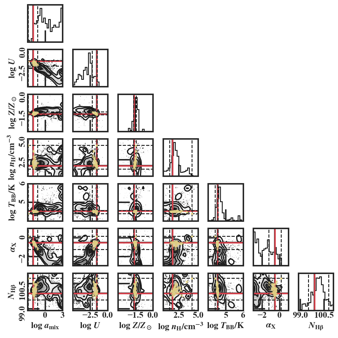
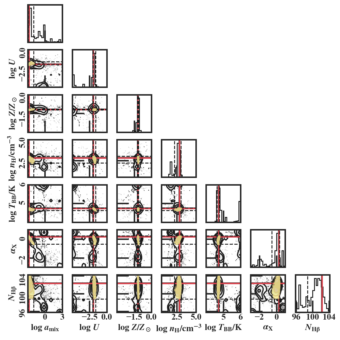
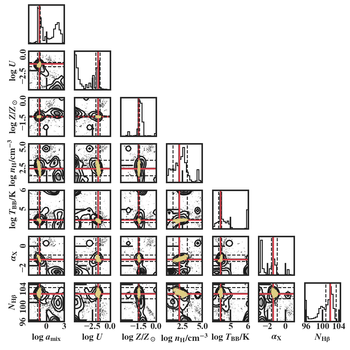
In Figure 2, 3, and 4, the prior ranges are wide enough to reveal the overall shapes of the PDFs that are not distorted by the prior boundaries except for that of $\log a_{\rm mix}$ of J104457. However, the uncertainty ranges for $\log a_{\rm mix}$ of J104457 are within its prior range. The PDF for some of the parameters has multi-modal distribution. In contrast, parameter sets within the uncertainty ranges (yellow dots) are concentrated around the best-fit parameters. This suggests that peaks other than those of the best-fit parameters are just local maxima of equation 6. The best-fit values for metallicity of our three galaxies are comparable (within 0.2 dex) with the literature values of metallicity.

3.2 Reproduction of Emission Lines

Table 4: Best Fit Parameters

	Parameters	J1631+4426	J104457	I Zw 18 NW
Best Fit Parameters
(1)	$\log a_{\rm mix}$	$-2.05^{+0.74}_{-0.84}$	$-2.81^{+0.83}_{-0.08}$	$-1.18^{+0.14}_{-0.35}$
(2)	$\log T_{\rm BB}/{\rm K}$	$4.54^{+0.02}_{-0.14}$	$4.74^{+0.03}_{-0.11}$	$4.45^{+0.05}_{-0.12}$
(3)	$\alpha_{\rm X}$	$-0.53^{+0.70}_{-0.71}$	$0.26^{+0.09}_{-0.80}$	$-1.37^{+0.45}_{-0.20}$
(4)	$\log U$	$-1.55^{+0.05}_{-0.68}$	$-1.95^{+0.34}_{-0.07}$	$-1.67^{+0.22}_{-0.34}$
(5)	$\log n_{\rm H}/{\rm cm^{-3}}$	$1.74^{+2.48}_{-0.39}$	$2.82^{+0.19}_{-0.63}$	$2.12^{+0.97}_{-0.82}$
(6)	$\log Z/Z_{\odot}$	$-1.61^{+0.19}_{-0.05}$	$-1.19^{+0.05}_{-0.03}$	$-1.48^{+0.07}_{-0.05}$
(7)	$\mathit{N}_{{\rm H}\beta}$	$99.9^{+0.9}_{-0.4}$	$102.3^{+1.9}_{-3.5}$	$101.9^{+1.4}_{-1.1}$

Note. — Best fit parameters are the sampled parameters that maximize $\log\mathcal{L}$ in equation (6). Uncertainties for best fit parameters are derived from condition shown in equation (LABEL:uncert). (1): Ratio of blackbody flux to power-law flux at 1 Ryd. (2): Blackbody temperature. (3): Power law index. (4): Ionization parameter. (5): Hydrogen density. (6): Gas-phase metallicity. (7): Normalization factor for an H$\beta$ emission line. (i.e., model emission line flux for H$\beta$). Here, the observed H$\beta$ emission line flux values are normalized at 100.

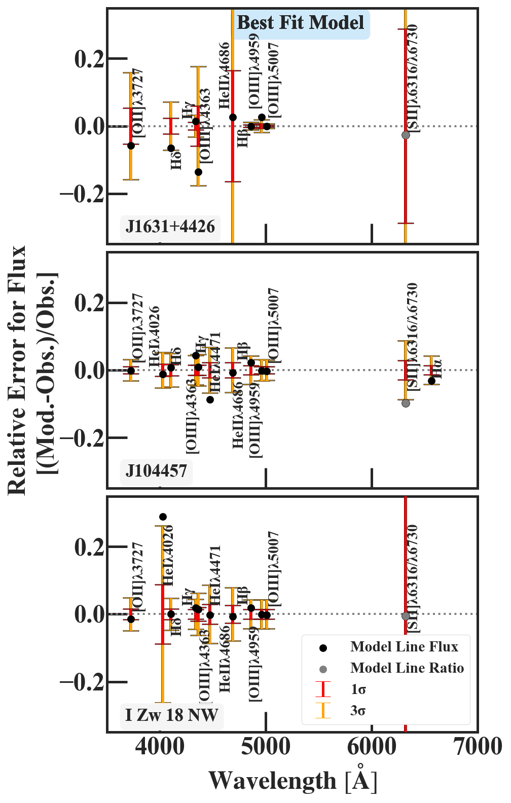
We compare the observed emission line fluxes with the model emission line fluxes reproduced with the best-fit parameters. In Figure 5, we present normalized differences between the observed and the model fluxes for emission lines in the black dots. We also plot the $1\sigma_{\lambda,\rm{obs}}$ and $3\sigma_{\lambda,\rm{obs}}$ ranges for the emission lines in the red and yellow bars, respectively. From Figure 5, we find that the best-fit models simultaneously reproduce all the emission lines within around $3\sigma_{\lambda,\rm{obs}}$ for all of our three galaxies. Interestingly, [O iii]$\lambda$4363 is the most deviant line for J1631+4426. This deviance is probably because our current model for the MCMC method could be weighting too much on reproducing [O iii]$\lambda$$\lambda$4959,5007. The 1$\sigma$ values for [O iii]$\lambda$$\lambda$4959,5007 are below 1% of the flux values, while 1$\sigma$ values for [O iii]$\lambda$4363 is about 5% of the flux value.

Figure 5: Emission line fluxes and flux ratios reproduced from the best-fit parameters. We show results for J1631+4426 (top), J104457 (middle), and I Zw 18 NW (bottom). The relative errors for fluxes (black dots) are differences between the value produced from the best-fit parameters and the observed values, normalized by the observed values. The red (yellow) bars represent the $1\sigma$ ($3\sigma$) errors of the observed values.

3.3 Ionizing Spectrum Shapes

In Figure 6, we depict the general ionizing spectrum shapes reproduced from the best-fit parameters for our three galaxies . Hereafter, we call these ionizing spectra as the “best-fit” ionizing spectra. For comparison, we overplot the ionizing spectrum of the BPASS binary model at the stellar age 10 Myr and the stellar metallicity $Z_{*}$ at $0.05~{}Z_{\odot}$. We use BPASS v2.2.1 (Eldridge et al., 2017; Stanway & Eldridge, 2018) with a Kroupa initial mass function (IMF) and a high mass cut-off at $300~{}M_{\odot}$. All ionizing spectra are normalized at 910 Å. We also plot uncertainties for the spectral fluxes at ionization energies of ions used in our parameter search. The uncertainty bars are given by the maximum and the minimum spectral flux values reproduced with the sampled parameter sets satisfying equation LABEL:uncert. We note again that these uncertainties are only rough standards and the actual uncertainties could be be more strictly given.

Figure 6: Ionizing spectrum shapes reproduced for J1631+4426 (red line), J104457 (blue line), and I Zw 18 NW (orange line) with our MCMC methods. The grey line is an example ionizing spectrum from the BPASS binary model (${\rm Age}=10~{}{\rm Myr},~{}Z_{*}=0.05Z_{\odot}$). The vertical dotted lines mark the ionization energies of ${\rm H^{0}}$, ${\rm O^{0}}$, ${\rm He^{0}}$, ${\rm O^{+}}$, and ${\rm He^{+}}$. The colored dot (bar) represents the value of flux (the range of uncertainty) at each ionization energy for the best-fit ionizing spectra. The black cross represents the value of flux at each ionization energy for the BPASS binary model. All ionizing spectra are normalized at $910~{}$Å

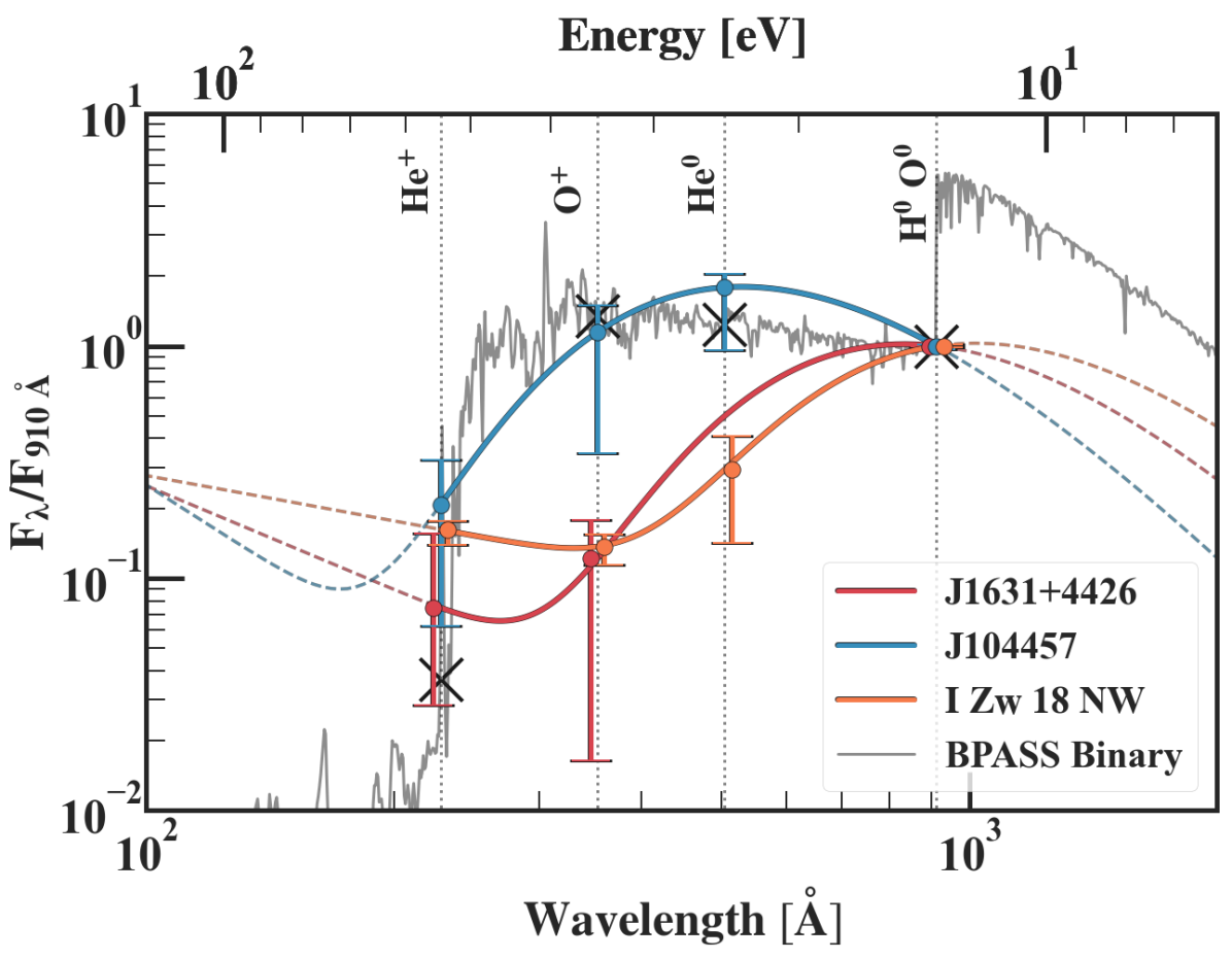
Between the ionization energies of ${\rm H^{0}}$ $(13.6~{}{\rm eV})$ and ${\rm He^{+}}$ $(54.4~{}{\rm eV})$, we find that the best-fit ionizing spectra have two types of general spectrum shapes. The best-fit ionizing spectrum for J104457 has a convex upward spectrum shape like the one for BPASS binary models, except that most of the He ii ionizing photons are absorbed by the stellar atmosphere in the BPASS binary models. On the other hand, the best-fit ionizing spectra for J1631+4426 and I Zw 18 NW have convex downward spectrum shapes that BPASS binary models cannot reproduce. These convex downward spectrum shapes have dominant contributions from the power-law radiation around the ionization energy of ${\rm He}^{+}~{}(54.4~{}{\rm eV})$. These two types of general spectrum shapes indicate a diversity of the ionizing spectrum shapes for EMPGs.

3.4 Comparison with Other Models

O21 claim that the combination of a BPASS binary model and blackbody radiation can reproduce emission lines from J104457 in a self-consistent manner. We compare our self-consistent model for J104457 with the model for J104457 presented in O21. We construct a mock model for the model presented O21 using the model parameters listed in the bottom column of Table 5 in the same paper. We use the same BPASS version and initial mass function as O21 for the mock model. In Figure 7 (a), we present a spectrum of the mock model in the blue line, the spectrum from O21 in the green line, and our result for J104457 in the red solid line. Only the spectrum for below 54.4 eV is shown for the model in O21. We find that the spectrum in O21 has relatively higher fluxes around 54.4 eV than the spectrum of our result.

Figure 7: Comparison between our result for J104457 and other models. (a) The blue, green, red solid, and red dashed lines are the spectrum of the mock model for O21, the model in O21, our result for J104457, and our result when we include [Ne v]$\lambda$3426/[Ne iii]$\lambda$3869, respectively. Only the spectrum below 54.4 eV is shown for the model in O21. The other symbols are the same as those in Figure 6. (b) Emission line fluxes and emission line ratios from two models. The blue (back) dots are the emission line fluxes and emission line ratio from the mock model of O21 (our result for J104457). The other symbols are the same as those in Figure 5.

In Figure 7 (b), we show emission line fluxes and emission line ratios for the mock model (our model) in blue (black) dots. The mock model of O21 reproduces the observed He ii$\lambda$4686 fairly well. However, other emission lines, especially the low-ionization emission line fluxes such as [O ii]$\lambda$$\lambda$3727,3729, He i$\lambda$4026, and He i$\lambda$4471, are systematically underproduced, unlike our result. One possible explanation for this underproduction by the mock model is that the general spectrum shape for the mock model has a relatively lower ratio of low-energy ($13.6-24.6$ eV) fluxes to high-energy ($35.1-54.4$ eV) fluxes than that of our result.

Next, we consider how taking [Ne v] emission lines into consideration affects our result. [Ne v] emission lines are detected in some of the He ii emitting EMPGs including J104457 (e.g., Izotov et al., 2004; Senchyna et al., 2017; Isobe et al., 2021a; Izotov et al., 2021b). Because [Ne v] is a very-high ionization line with an ionization potential of 97.1 eV, its relative flux to H$\beta$ can be used to constrain the contribution of very hard (i.e., X-ray) radiation to the ionizing spectrum shapes (e.g., Lebouteiller et al., 2017; Senchyna et al., 2020; Simmonds et al., 2021). Simmonds et al. (2021) show that some ULX models can reproduce He ii$\lambda$4686 and [Ne v]$\lambda$3426 flux values that are comparable to those from observations.

We conduct the same method as described in 2, but add [Ne v]$\lambda$3426 into consideration. We only examine for J104457 because [Ne v] emission lines are not detected in the other two galaxies, most likely due to the lack of sensitivity. To avoid uncertainty in abundance ratio, we use [Ne v]$\lambda$3426/[Ne iii]$\lambda$3869 as we have done to [S ii]$\lambda$$\lambda$6316,6731. The observed [Ne v]$\lambda$3426/[Ne iii]$\lambda$3869 value and its 1$\sigma$ error for J104457 are $0.00347\pm 0.00315$ (B21). We obtain similar best-fit values for each parameter from MCMC. In Figure 7, we have overplotted the ionizing spectrum produced from the parameter in Table 5 as the red dashed line. Although the blackbody component has a higher temperature, the newly obtained ionizing spectrum generally has a similar spectrum shape as the one we obtain without considering [Ne v]$\lambda$3426/[Ne iii]$\lambda$3869. [Ne v]$\lambda$3426/[Ne iii]$\lambda$3869 value produced from new ionizing spectrum shapes is produced within around 3$\sigma$ of the observed value. Moreover, this new ionizing spectrum shape produces other emission lines within around 3$\sigma$. Therefore, we confirm that the general spectrum shape for J104457 is consistent with [Ne v]$\lambda$3426, which requires very high energy ($>97.1$ eV) ionizing photons.

Table 5: Best Fit Parameters with [Ne v] for J104457

	Parameters	Best Fit Values
(1)	$\log a_{\rm mix}$	$-2.97$
(2)	$\log T_{\rm BB}/{\rm K}$	$4.80$
(3)	$\alpha_{\rm X}$	$0.37$
(4)	$\log U$	$-2.05$
(5)	$\log n_{\rm H}/{\rm cm^{-3}}$	$2.84$
(6)	$\log Z/Z_{\odot}$	$-1.16$
(7)	$\mathit{N}_{{\rm H}\beta}$	$102.8$

Note. — (1): Ratio of the blackbody flux to the power-law flux at 1 Ryd. (2): Blackbody temperature. (3): Power law index. (4): Ionization parameter. (5): Hydrogen density. (6): Gas-phase metallicity. (7): Normalization factor for an H$\beta$ emission line. The best fit values listed in this table are obtained with the analysis described in Section 2 but with taking [Ne v]$\lambda$3462/[Ne iii]$\lambda$3869 into consideration.

4 Discussion

4.1 Contributions from Stellar Radiation

Our best-fit ionizing spectra have blackbody temperature around $3-5\times 10^{4}~{}{\rm K}$. B-type (O-type) stars have surface temperature of $1-3\times 10^{4}~{}{\rm K}$ ($\geq 3\times 10^{4}~{}{\rm K}$). This suggests that blackbody radiation in our best-fit ionizing spectra, especially for that of J104457, can be explained by B- and O-type stars. However, the convex downward spectra of J1631+4426 and I Zw 18 NW suggest that contributions from stars to hard photons around 35.1 to 54.4 eV might not be as significant as expected in BPASS binary models. Stellar models including fast-rotating stars (e.g., Kubátová et al., 2019) and population III stars (e.g., Grisdale et al., 2021) also have convex upward spectra around $13.6-54.4$ eV, unlike our results. These mismatches suggest that hard radiation from stellar sources cannot solely explain He ii ionizing photons for the two of our galaxies with convex downward spectrum shapes.

We also note that our general spectrum shapes do not take account of stellar absorptions. Stellar absorptions weaken intrinsic stellar radiation above ionization energies of ${\rm H^{0}}$ (13.6 eV), ${\rm He^{0}}$ (24.6 eV), and ${\rm He^{+}}$ (54.4 eV). This raises the question of whether stellar models with stellar absorption can really reproduce ionizing spectra of our three galaxies including the blackbody-dominated spectra of J104457. More sophisticated spectral modeling is needed to further examine the stellar contributions, but this is beyond the scope of our paper.

4.2 Contributions from Black Holes

We examine the contributions from black holes (BHs) such as AGNs and HMXBs/ULXs. BHs can produce very hard radiation through non-thermal radiation from Comptonization/synchrotron radiation. Because non-thermal radiation has a power-law-like shape, radiation from BH could explain the power-law-like component seen in the ionizing spectrum of J1631+4426 and I Zw 18 NW. BH radiation also has hot ($\gtrsim 10^{5}~{}{\rm K}$) thermal radiation from their accretion disks. Temperatures of accretion disks are roughly proportional to $M_{\rm BH}^{-1/4}$, where $M_{\rm BH}$ is the mass of BH. Following the relation between the accretion disk temperature and $M_{\rm BH}$, intermediate-mass BHs ($10^{2}\leq M_{\rm BH}\leq 10^{5}~{}M_{\odot}$) and less massive ones would not produce sufficient ionizing photons in the soft energy range of $<54.4$ eV. For this reason, we will first examine if AGN can solely account for the general spectrum shapes of our three galaxies by comparing them with spectra of AGNs. Then, we will investigate whether the combinations of a BH and stellar population can explain the general spectrum shapes of our three galaxies.

4.2.1 Only BHs

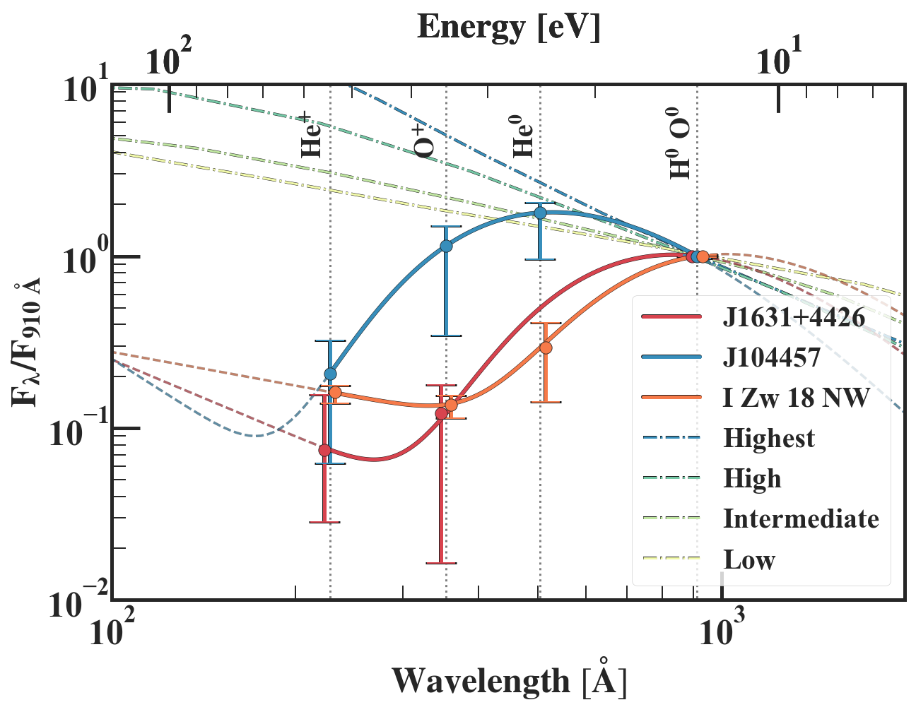
The inner-disk temperature $T_{\rm in}$ of the accretion disk is around $10^{4-5}~{}{\rm K}$ for AGNs. The blackbody radiation from the inner disk of an AGN gives a Big Blue Bump (BBB) feature in the UV range of the ionizing spectrum. The BBB feature combined with non-thermal radiation can produce a spectrum shape like the one reproduced from the combination of a blackbody and power-law radiation. We compare the shapes of four different AGN spectra with the general spectrum shapes of our three galaxies in Figure 8. These four AGN spectra are taken from Ferland et al. (2020), and they represent mean spectra of observed Type-1 AGNs grouped by Eddington ratios (Highest, High, Intermediate, and Low). As shown in Figure 8, all four AGN spectra have power-law like shapes between $13.6-54.4$ eV, unlike the ionizing spectra of our three galaxies. The deformation of disk-blackbody by the Compotonization in observed AGN might be the reason why AGN spectra does not have blackbody-like shapes in $13.6-54.4$ eV (see Ferland et al., 2020). From this comparison, we cannot conclude that AGN can solely explain the general spectrum shapes for our three galaxies. However, we note that ionizing spectrum shapes of AGNs remain unclear especially around the Lyman limit to soft X-ray because of the intervening absorption.

Figure 8: Comparison of our result with AGN spectra. The dash-dotted lines represent mean AGN spectra by different Eddington ratios (Highest, High, Intermediate, and Low) taken from Ferland et al. (2020). The other symbols are the same as those in Figure 6.

4.2.2 BHs and Stars

We will explore the combinations of BHs and stellar sources to see if they can account for the general spectrum shapes of our three galaxies. We choose ULXs as non-stellar sources because they are popular candidates for the origin of He ii. Moreover, there are detections of a ULX in I Zw 18 through X-ray observations (e.g., Kaaret & Feng, 2013). As a ULX spectrum, we use a spectral model described in Gierliński et al. (2009). According to Simmonds et al. (2021), this ULX spectral model reproduces emission line ratios in metal-poor galaxies better than other ULX spectral models. We produce the ULX spectrum models from numerical calculations. To run the numerical calculations, we have referred to the code of the DISKIR model provided in xspec (Arnaud, 1996). As presented in Simmonds et al. (2021), ULX spectral models cannot produce enough photons in UV region, we combine ULX spectral model with stellar spectral model (hereafter ULX $+$ BPASS single model). We use spectra reproduced from BPASS single star models as stellar spectra. We assume single-aged stellar population with the same IMF as the BPASS binary model we presented in Figure 6. We do not use BPASS binary models because adding extra hard components from ULX would not alter the convex upward spectrum shape of the spectra reproduced from BPASS binary models. We use fluxes at the ionization energies of ${\rm H^{0}}$, ${\rm He^{0}}$, ${\rm O^{+}}$, and ${\rm He^{+}}$ for the best-fit ionizing spectra to restrict the ULX $+$ BPASS single models for our three galaxies. We allow a stellar age $t$ and a ratio between $0.5-8$ keV X-ray luminosity $L_{\rm X}$ and SFR ($L_{\rm X}/{\rm SFR}$) to vary. A SFR for $L_{\rm X}/{\rm SFR}$ is calculated from UV luminosity at 1500 Å using relationships presented in Kennicutt (1998). For each of our three galaxies, we fix the value of stellar metallicity $Z_{*}$ at the best-fit value of gas-phase metallicity.

Table 6: Parameters for ULX + BPASS Single Models

Name of the Galaxy	$t$	$\log L_{{\rm X}}/{\rm SFR}$
	(Myr)	(erg s-1/$M_{\odot}\,{\rm yr}^{-1}$)
	(1)	(2)
J1631+4426	$8.2$	$40.7$
J104457	$2.2$	$41.5$
I Zw 18 NW	$8.5$	$41.0$

Note. — (1): Stellar Age. We assume a single-aged stellar populations. (2): $0.5-8$ keV X-ray luminosity to SFR.

Figure 9: ULX+BPASS single models for J1631+4426 (red thin line), J104457 (blue thin line), and I Zw 18 NW (orange thin line). The other symbols are the same as those in Figure 6.

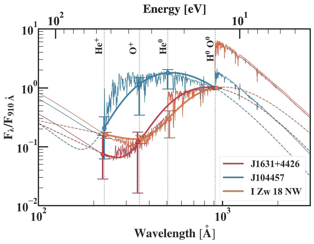
In Table 6, we summarize the parameters of the ULX + BPASS single models that reproduce the general spectrum shapes for our three galaxies. We compare the general spectrum shapes with the ULX + BPASS single star models in Figure 9. The spectrum of ULX + BPASS single star models for J1631+4426, J104457, and I Zw 18 NW are represented by the red, blue, and orange thin lines, respectively. We successfully reproduce the general spectrum shape of the best-fit ionizing spectra between $13.6-54.4$ eV for our three galaxies, despite the diversity in the general spectrum shapes. For both types of the spectrum shapes, the $L_{\rm X}/{\rm SFR}$ values are $\lesssim 10^{41}~{}{\rm ergs^{-1}/M_{\odot}{yr}^{-1}}$, which are comparable to the values obtained in Simmonds et al. (2021). The blackbody-like spectrum shape of J104457 can be explained by prominent stellar contributions relative to that of the ULX, while the convex downward spectrum shapes of J1631+4426 and I Zw 18 NW can be explained by the less prominent stellar contributions around $35.1-54.4$ eV than that of J104457. Moreover, the stellar component for J104457 has the stellar age around 2 Myr, while the stellar components for J1631+4426 and I Zw 18 NW have the stellar age above 5 Myr. This suggests that the diversity of the spectrum shapes can arises from the stellar age difference of the stellar components. The stellar contributions become less prominent at $\gtrsim$ 5 Myr because massive stars with their mass at $\gtrsim 40~{}M_{\odot}$ already reach their lifetimes (Xiao et al., 2018).

4.3 Other Possibilities

We have only examined ULX as the non-stellar component when considering the combination with the stellar component, but it does not limit the possibilities of other sources such as low luminosity AGNs and supersoft X-ray sources. Photoionization by shocks is still not ruled out from the candidate by our analysis. The ionization of He ii by soft X-rays from cluster winds and superbubbles also remains a possibility (see Oskinova & Schaerer, 2022). Further X-ray observations for J1631+4426 and J104457 may enable us to constrain contributions from X-ray emitting sources.

4.4 Multi-Wavelength Comparison and Relation with Cosmic Reionization

Figure 10: Comparison between the multi-wavelength data and our models for I Zw 18. The black diamonds represent the unfolded X-ray luminosities. The leftward (rightward) black circle represents the $i^{\prime}$- ($z^{\prime}$-) band magnitudes. The yellow (green) line represents the ionizing spectrum (net transmitted spectrum) of the comparison model. We also overplot the ionizing spectrum of I Zw 18NW in Figure 6 (BB+PL, orange line) under an assumption that the whole system has the same spectral shape. The other symbols are the same as those in Figure 6.

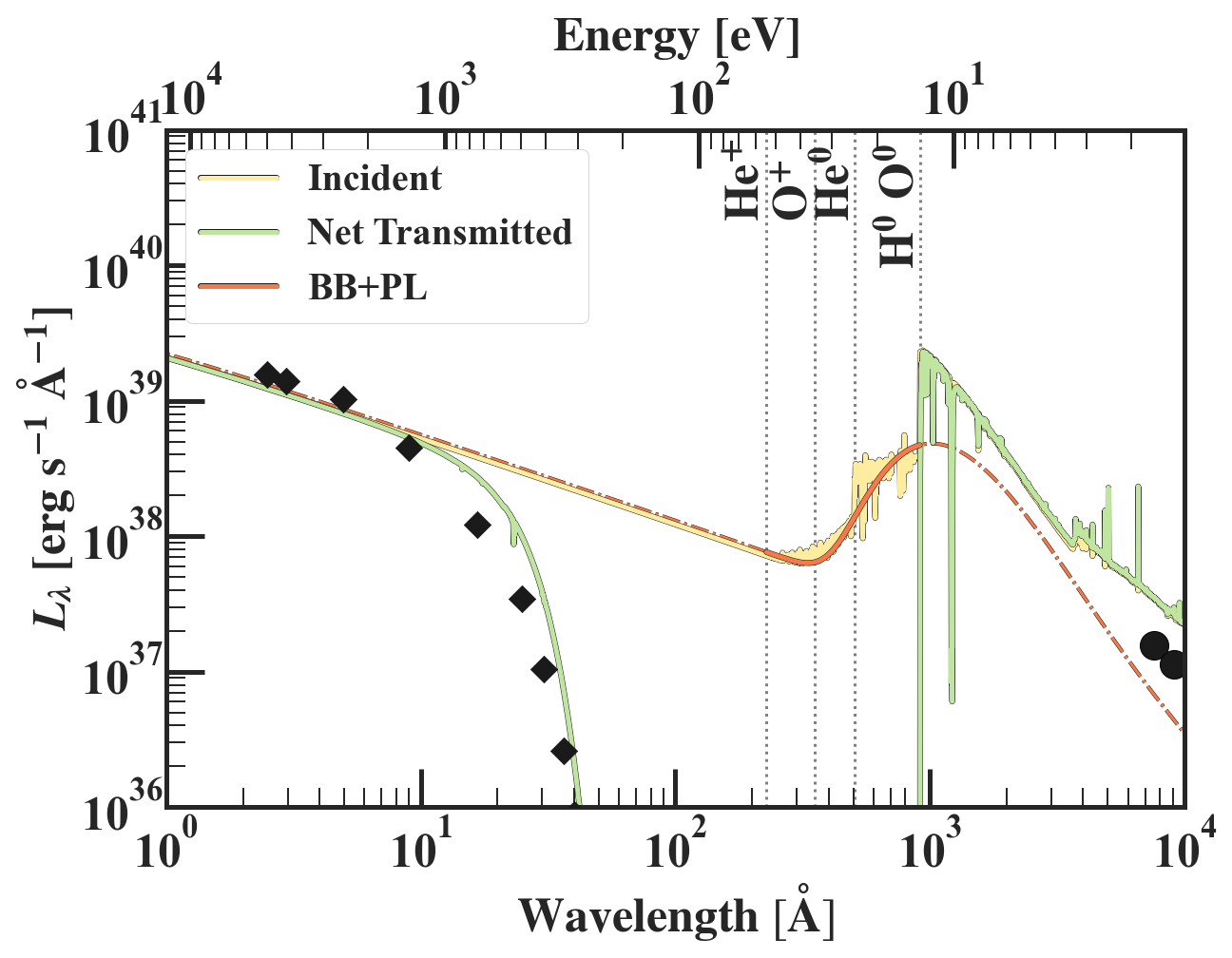
We investigate the consistency between our ionizing spectrum shapes and the observed values of I Zw 18, where multi-wavelength data from the X-ray to optical photometry data are available. We assume that whole I Zw 18 has the same ionizing spectrum shape as our result for I Zw 18 NW to compare the model with the observed values of I Zw 18 as a whole. We use the X-ray luminosity obtained by the X-ray Multi-Mirror Mission (XMM-Newton) (Kaaret & Feng, 2013; Lebouteiller et al., 2017). For optical photometry, we use SDSS $i^{\prime}$- and $z^{\prime}$-band magnitudes from DR16 (Ahumada et al., 2020) for I Zw 18 NW and I Zw 18 SE to compare the fluxes of the continuum. We do not use photometry data in other bands, where many strong emission lines are detected. To compare the optical photometry data, we replace the blackbody component of the ionizing spectrum with the BPASS single star model reproduced with the parameters for I Zw 18 NW in Table 6. We normalize the luminosity by adopting a distance of 18.2 Mpc (Aloisi et al., 2007), H$\beta$ luminosity of $10^{39.43}$ erg s^-1, and a relation between the number of hydrogen ionizing photons produced per second and the H$\beta$ luminosity presented in Ono et al. (2010). We show the comparison between the multi-wavelength data and the comparison model in Figure 10. The black diamonds represent unfolded X-ray luminosities and the leftward (rightward) black circle represents the $i^{\prime}$- ($z^{\prime}$-) band magnitude. The incident (net transmitted) spectrum of the comparison model is shown in the yellow (green) line. Here, the net transmitted spectrum is the sum of attenuated incident radiation and the outward portion of the emitted continuum and lines. The orange line is the same ionizing spectrum for I Zw 18 NW as the one presented in Figure 6. From Figure 10, we find that the optical photometry data is slightly below what our comparison model predicts. However, the net transmitted spectrum of our comparison model is consistent with the X-ray luminosities.

Figure 11: Cumulative fraction of the hydrogen ionizing photon numbers at energies (red line) above the ionization energy of ${\rm H^{0}}$ (13.6 eV) for our spectrum model. The dotted lines mark the ionization energies of ${\rm H}^{0}$, ${\rm O}^{0}$. ${\rm He}^{0}$, ${\rm O}^{+}$, and ${\rm He}^{+}$. The cumulative fraction of the ionizing photon numbers at the ionization energy of ${\rm He^{0}}$ (24.6 eV) already reaches $\sim 90\%$ (dashed line). The cumulative fraction at the ionization energy of ${\rm He^{+}}$ (54.4 eV) exceeds $97\%$ (dotted-dashed line).

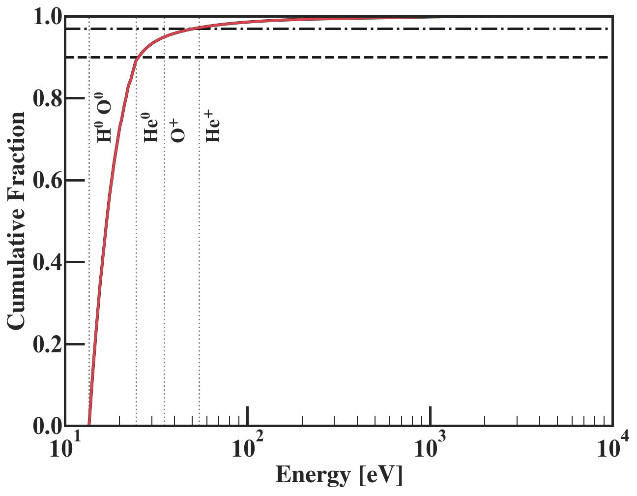
As described in Section 1, a nearby EMPG can be a probe for young galaxies at EoR. We evaluate the contribution of X-ray photons from the young galaxies to cosmic reionization, assuming that the young galaxies have the same ionizing spectrum shapes as the spectrum of I Zw 18. We adjust the ionizing photon escape fraction of 20% to match the standard picture of cosmic reionization (e.g., Ouchi et al., 2009; Robertson et al., 2013). To do so, we consider the model spectrum that linearly combines the incident ionizing spectrum and the net transmitted spectrum with their luminosities multiplied by 0.2 and 0.8, respectively. In Figure 11, we depict the cumulative fraction of the hydrogen ionizing photon number at each energy in the red line. As shown in Figure 11, about $90\%$ ($97\%$) of the ionizing photons have energy below 24.6 eV (54.4 eV). Moreover, the contributions of the high energy ($>$54.4 eV) photons would be further reduced because the photoionization cross-section has the photon energy dependency of approximately $E^{-3}$ (Osterbrock & Ferland, 2006). Thus, we conclude that the hard ionizing radiation does not affect the standard picture of cosmic reionization (Robertson, 2021).

5 Conclusions

We have searched for the general spectrum shapes of ionizing sources in EMPGs that can explain major emission lines including He ii. We have prepared parameterized ionizing spectra with generalized shapes, and use these ionizing spectra in photoionization models with free parameters of ionizing spectra and nebulae. For three EMPGs with strong He ii$\lambda$4686, we have determined seven parameters of the ionizing spectra and nebulae using MCMC methods.

Our main findings can be summarized as follows:

1. We have determined the best-fit parameters for our three galaxies. All the best-fit parameters are comparable to ordinary values. With the best-fit parameters, we successfully reproduced all major emission lines within $\lesssim 3\sigma$ errors.

2. The ionizing spectrum produced from the best-fit parameters for J104457 has a blackbody-dominated shape around $13.6-54.4$ eV with blackbody temperature $5\times 10^{4}$ K. In contrast, the ionizing spectra for J1631+4426 and I Zw 18 NW have significant contributions from power-law radiation around 54.4 eV, with relatively low-temperature ($3\times 10^{4}$ K) blackbody radiation. As a result, the general spectrum shapes for J1631+4426 and I Zw 18 NW have convex downward shapes around $13.6-54.4$ eV, which are fundamentally different from the shapes predicted by BPASS binary models. These two types of spectrum shapes indicate a diversity in ionizing spectrum shapes in EMPGs.

3. We compare obtained general shapes of ionizing spectra with that of ionizing spectra from stars, AGNs, and ULXs. We find that ULX $+$ BPASS single star models can explain the general shapes of the obtained ionizing spectra for our three galaxies. Furthermore, we show that the diversity of the spectrum shapes can be attributed to the differences in the stellar age.

4. We confirm that our result is consistent with the X-ray to optical photometry data for I Zw 18, of which the multi-wavelength data are available. We also find that the hard ionizing radiation inferred from our general spectrum shape of I Zw 18 does not contradict the standard picture of cosmic reionization.

Spectroscopic observation of J1631+4426 and I Zw 18 NW for optical [Ne v] emission lines with high sensitivity would also be helpful in terms of constraining contributions of ionizing photons $\gtrsim 100$ eV in He ii emissions. Our new analysis method would provide new insights into the statistical nature of EMPGs if applied to the sample with a large number of EMPGs.

References

- Abazajian et al. (2004) Abazajian, K., Adelman-McCarthy, J. K., Agüeros, M. A., et al. 2004, AJ, 128, 502, doi: 10.1086/421365
- Abazajian et al. (2009) Abazajian, K. N., Adelman-McCarthy, J. K., Agüeros, M. A., et al. 2009, ApJS, 182, 543, doi: 10.1088/0067-0049/182/2/543
- Adelman-McCarthy et al. (2008) Adelman-McCarthy, J. K., Agüeros, M. A., Allam, S. S., et al. 2008, ApJS, 175, 297, doi: 10.1086/524984
- Ahumada et al. (2020) Ahumada, R., Prieto, C. A., Almeida, A., et al. 2020, ApJS, 249, 3, doi: 10.3847/1538-4365/ab929e
- Alavi et al. (2020) Alavi, A., Colbert, J., Teplitz, H. I., et al. 2020, ApJ, 904, 59, doi: 10.3847/1538-4357/abbd43
- Allen et al. (2008) Allen, M. G., Groves, B. A., Dopita, M. A., Sutherland, R. S., & Kewley, L. J. 2008, ApJS, 178, 20, doi: 10.1086/589652
- Aloisi et al. (2007) Aloisi, A., Clementini, G., Tosi, M., et al. 2007, ApJ, 667, L151, doi: 10.1086/522368
- Arnaud (1996) Arnaud, K. A. 1996, in Astronomical Society of the Pacific Conference Series, Vol. 101, Astronomical Data Analysis Software and Systems V, ed. G. H. Jacoby & J. Barnes, 17
- Asplund et al. (2009) Asplund, M., Grevesse, N., Sauval, A. J., & Scott, P. 2009, ARA&A, 47, 481, doi: 10.1146/annurev.astro.46.060407.145222
- Atek et al. (2018) Atek, H., Richard, J., Kneib, J.-P., & Schaerer, D. 2018, MNRAS, 479, 5184, doi: 10.1093/mnras/sty1820
- Baldwin et al. (1981) Baldwin, J. A., Phillips, M. M., & Terlevich, R. 1981, PASP, 93, 5, doi: 10.1086/130766
- Berg et al. (2019) Berg, D. A., Chisholm, J., Erb, D. K., et al. 2019, ApJ, 878, L3, doi: 10.3847/2041-8213/ab21dc
- Berg et al. (2021) —. 2021, arXiv e-prints, arXiv:2105.12765. https://arxiv.org/abs/2105.12765
- Berg et al. (2018) Berg, D. A., Erb, D. K., Auger, M. W., Pettini, M., & Brammer, G. B. 2018, ApJ, 859, 164, doi: 10.3847/1538-4357/aab7fa
- Bouwens et al. (2015) Bouwens, R. J., Illingworth, G. D., Oesch, P. A., et al. 2015, ApJ, 811, 140, doi: 10.1088/0004-637X/811/2/140
- Dopita et al. (2006) Dopita, M. A., Fischera, J., Sutherland, R. S., et al. 2006, ApJS, 167, 177, doi: 10.1086/508261
- Eldridge et al. (2017) Eldridge, J. J., Stanway, E. R., Xiao, L., et al. 2017, PASA, 34, e058, doi: 10.1017/pasa.2017.51
- Ferland et al. (2020) Ferland, G. J., Done, C., Jin, C., Landt, H., & Ward, M. J. 2020, MNRAS, 494, 5917, doi: 10.1093/mnras/staa1207
- Ferland et al. (2013) Ferland, G. J., Porter, R. L., van Hoof, P. A. M., et al. 2013, Rev. Mexicana Astron. Astrofis., 49, 137. https://arxiv.org/abs/1302.4485
- Ferland et al. (2017) Ferland, G. J., Chatzikos, M., Guzmán, F., et al. 2017, Rev. Mexicana Astron. Astrofis., 53, 385. https://arxiv.org/abs/1705.10877
- Fernández et al. (2021) Fernández, V., Amorín, R., Pérez-Montero, E., et al. 2021, MNRAS, doi: 10.1093/mnras/stab3150
- Gierliński et al. (2009) Gierliński, M., Done, C., & Page, K. 2009, MNRAS, 392, 1106, doi: 10.1111/j.1365-2966.2008.14166.x
- Grevesse et al. (2010) Grevesse, N., Asplund, M., Sauval, A. J., & Scott, P. 2010, Ap&SS, 328, 179, doi: 10.1007/s10509-010-0288-z
- Grisdale et al. (2021) Grisdale, K., Thatte, N., Devriendt, J., et al. 2021, MNRAS, 501, 5517, doi: 10.1093/mnras/stab013
- Guseva et al. (2000) Guseva, N. G., Izotov, Y. I., & Thuan, T. X. 2000, ApJ, 531, 776, doi: 10.1086/308489
- Harikane et al. (2016) Harikane, Y., Ouchi, M., Ono, Y., et al. 2016, ApJ, 821, 123, doi: 10.3847/0004-637X/821/2/123
- Isobe et al. (2021a) Isobe, Y., Ouchi, M., Suzuki, A., et al. 2021a, arXiv e-prints, arXiv:2108.03850. https://arxiv.org/abs/2108.03850
- Isobe et al. (2021b) Isobe, Y., Ouchi, M., Kojima, T., et al. 2021b, ApJ, 918, 54, doi: 10.3847/1538-4357/ac05bf
- Izotov et al. (2004) Izotov, Y. I., Noeske, K. G., Guseva, N. G., et al. 2004, A&A, 415, L27, doi: 10.1051/0004-6361:20040006
- Izotov & Thuan (1998) Izotov, Y. I., & Thuan, T. X. 1998, ApJ, 497, 227, doi: 10.1086/305440
- Izotov et al. (2021a) Izotov, Y. I., Thuan, T. X., & Guseva, N. G. 2021a, MNRAS, doi: 10.1093/mnras/stab2798
- Izotov et al. (2021b) —. 2021b, MNRAS, 508, 2556, doi: 10.1093/mnras/stab2798
- Izotov et al. (2021c) Izotov, Y. I., Worseck, G., Schaerer, D., et al. 2021c, MNRAS, 503, 1734, doi: 10.1093/mnras/stab612
- Kaaret & Feng (2013) Kaaret, P., & Feng, H. 2013, ApJ, 770, 20, doi: 10.1088/0004-637X/770/1/20
- Kauffmann et al. (2003) Kauffmann, G., Heckman, T. M., Tremonti, C., et al. 2003, MNRAS, 346, 1055, doi: 10.1111/j.1365-2966.2003.07154.x
- Kehrig et al. (2021) Kehrig, C., Guerrero, M. A., Vílchez, J. M., & Ramos-Larios, G. 2021, ApJ, 908, L54, doi: 10.3847/2041-8213/abe41b
- Kehrig et al. (2018) Kehrig, C., Vílchez, J. M., Guerrero, M. A., et al. 2018, MNRAS, 480, 1081, doi: 10.1093/mnras/sty1920
- Kennicutt (1998) Kennicutt, Robert C., J. 1998, ARA&A, 36, 189, doi: 10.1146/annurev.astro.36.1.189
- Kewley et al. (2013) Kewley, L. J., Dopita, M. A., Leitherer, C., et al. 2013, ApJ, 774, 100, doi: 10.1088/0004-637X/774/2/100
- Kikuchihara et al. (2020) Kikuchihara, S., Ouchi, M., Ono, Y., et al. 2020, ApJ, 893, 60, doi: 10.3847/1538-4357/ab7dbe
- Kojima et al. (2020) Kojima, T., Ouchi, M., Rauch, M., et al. 2020, ApJ, 898, 142, doi: 10.3847/1538-4357/aba047
- Kojima et al. (2021) —. 2021, ApJ, 913, 22, doi: 10.3847/1538-4357/abec3d
- Kubátová et al. (2019) Kubátová, B., Szécsi, D., Sander, A. A. C., et al. 2019, A&A, 623, A8, doi: 10.1051/0004-6361/201834360
- Laporte et al. (2017) Laporte, N., Nakajima, K., Ellis, R. S., et al. 2017, ApJ, 851, 40, doi: 10.3847/1538-4357/aa96a8
- Lebouteiller et al. (2017) Lebouteiller, V., Péquignot, D., Cormier, D., et al. 2017, A&A, 602, A45, doi: 10.1051/0004-6361/201629675
- Legrand et al. (1997) Legrand, F., Kunth, D., Roy, J. R., Mas-Hesse, J. M., & Walsh, J. R. 1997, A&A, 326, L17. https://arxiv.org/abs/astro-ph/9707279
- Livermore et al. (2017) Livermore, R. C., Finkelstein, S. L., & Lotz, J. M. 2017, ApJ, 835, 113, doi: 10.3847/1538-4357/835/2/113
- López-Sánchez et al. (2012) López-Sánchez, Á. R., Dopita, M. A., Kewley, L. J., et al. 2012, MNRAS, 426, 2630, doi: 10.1111/j.1365-2966.2012.21145.x
- López-Sánchez & Esteban (2010) López-Sánchez, Á. R., & Esteban, C. 2010, A&A, 516, A104, doi: 10.1051/0004-6361/200913434
- Madau & Haardt (2015) Madau, P., & Haardt, F. 2015, ApJ, 813, L8, doi: 10.1088/2041-8205/813/1/L8
- Mainali et al. (2018) Mainali, R., Zitrin, A., Stark, D. P., et al. 2018, MNRAS, 479, 1180, doi: 10.1093/mnras/sty1640
- Oesch et al. (2018) Oesch, P. A., Bouwens, R. J., Illingworth, G. D., Labbé, I., & Stefanon, M. 2018, ApJ, 855, 105, doi: 10.3847/1538-4357/aab03f
- Olivier et al. (2021) Olivier, G. M., Berg, D. A., Chisholm, J., et al. 2021, arXiv e-prints, arXiv:2109.06725. https://arxiv.org/abs/2109.06725
- Ono et al. (2010) Ono, Y., Ouchi, M., Shimasaku, K., et al. 2010, ApJ, 724, 1524, doi: 10.1088/0004-637X/724/2/1524
- Oskinova & Schaerer (2022) Oskinova, L., & Schaerer, D. 2022, arXiv e-prints, arXiv:2203.04987. https://arxiv.org/abs/2203.04987
- Osterbrock & Ferland (2006) Osterbrock, D. E., & Ferland, G. J. 2006, Astrophysics of gaseous nebulae and active galactic nuclei
- Ouchi et al. (2009) Ouchi, M., Mobasher, B., Shimasaku, K., et al. 2009, ApJ, 706, 1136, doi: 10.1088/0004-637X/706/2/1136
- Pérez-Montero et al. (2020) Pérez-Montero, E., Kehrig, C., Vílchez, J. M., et al. 2020, A&A, 643, A80, doi: 10.1051/0004-6361/202038509
- Plat et al. (2019) Plat, A., Charlot, S., Bruzual, G., et al. 2019, MNRAS, 490, 978, doi: 10.1093/mnras/stz2616
- Ramambason et al. (2020) Ramambason, L., Schaerer, D., Stasińska, G., et al. 2020, A&A, 644, A21, doi: 10.1051/0004-6361/202038634
- Rickards Vaught et al. (2021) Rickards Vaught, R. J., Sandstrom, K. M., & Hunt, L. K. 2021, ApJ, 911, L17, doi: 10.3847/2041-8213/abf09b
- Robertson (2021) Robertson, B. E. 2021, arXiv e-prints, arXiv:2110.13160. https://arxiv.org/abs/2110.13160
- Robertson et al. (2013) Robertson, B. E., Furlanetto, S. R., Schneider, E., et al. 2013, ApJ, 768, 71, doi: 10.1088/0004-637X/768/1/71
- Rutkowski et al. (2016) Rutkowski, M. J., Scarlata, C., Haardt, F., et al. 2016, ApJ, 819, 81, doi: 10.3847/0004-637X/819/1/81
- Sánchez Almeida et al. (2016) Sánchez Almeida, J., Pérez-Montero, E., Morales-Luis, A. B., et al. 2016, ApJ, 819, 110, doi: 10.3847/0004-637X/819/2/110
- Saxena et al. (2020) Saxena, A., Pentericci, L., Schaerer, D., et al. 2020, MNRAS, 496, 3796, doi: 10.1093/mnras/staa1805
- Saxena et al. (2022) Saxena, A., Pentericci, L., Ellis, R. S., et al. 2022, MNRAS, 511, 120, doi: 10.1093/mnras/stab3728
- Schaerer et al. (2019) Schaerer, D., Fragos, T., & Izotov, Y. I. 2019, A&A, 622, L10, doi: 10.1051/0004-6361/201935005
- Schmidt et al. (2017) Schmidt, K. B., Huang, K. H., Treu, T., et al. 2017, ApJ, 839, 17, doi: 10.3847/1538-4357/aa68a3
- Senchyna et al. (2020) Senchyna, P., Stark, D. P., Mirocha, J., et al. 2020, MNRAS, 494, 941, doi: 10.1093/mnras/staa586
- Senchyna et al. (2017) Senchyna, P., Stark, D. P., Vidal-García, A., et al. 2017, MNRAS, 472, 2608, doi: 10.1093/mnras/stx2059
- Shibuya et al. (2018) Shibuya, T., Ouchi, M., Harikane, Y., et al. 2018, PASJ, 70, S15, doi: 10.1093/pasj/psx107
- Shirazi & Brinchmann (2012) Shirazi, M., & Brinchmann, J. 2012, MNRAS, 421, 1043, doi: 10.1111/j.1365-2966.2012.20439.x
- Simmonds et al. (2021) Simmonds, C., Schaerer, D., & Verhamme, A. 2021, arXiv e-prints, arXiv:2108.12438. https://arxiv.org/abs/2108.12438
- Stanway & Eldridge (2018) Stanway, E. R., & Eldridge, J. J. 2018, MNRAS, 479, 75, doi: 10.1093/mnras/sty1353
- Stanway et al. (2016) Stanway, E. R., Eldridge, J. J., & Becker, G. D. 2016, MNRAS, 456, 485, doi: 10.1093/mnras/stv2661
- Stark et al. (2015) Stark, D. P., Richard, J., Charlot, S., et al. 2015, MNRAS, 450, 1846, doi: 10.1093/mnras/stv688
- Steidel et al. (2018) Steidel, C. C., Bogosavljević, M., Shapley, A. E., et al. 2018, ApJ, 869, 123, doi: 10.3847/1538-4357/aaed28
- Thuan et al. (2004) Thuan, T. X., Bauer, F. E., Papaderos, P., & Izotov, Y. I. 2004, ApJ, 606, 213, doi: 10.1086/382949
- Thuan & Izotov (2005) Thuan, T. X., & Izotov, Y. I. 2005, ApJS, 161, 240, doi: 10.1086/491657
- Thuan et al. (2005) Thuan, T. X., Lecavelier des Etangs, A., & Izotov, Y. I. 2005, ApJ, 621, 269, doi: 10.1086/427469
- Wise et al. (2014) Wise, J. H., Demchenko, V. G., Halicek, M. T., et al. 2014, MNRAS, 442, 2560, doi: 10.1093/mnras/stu979
- Wise et al. (2012) Wise, J. H., Turk, M. J., Norman, M. L., & Abel, T. 2012, ApJ, 745, 50, doi: 10.1088/0004-637X/745/1/50
- Xiao et al. (2018) Xiao, L., Stanway, E. R., & Eldridge, J. J. 2018, MNRAS, 477, 904, doi: 10.1093/mnras/sty646