Control of port-Hamiltonian differential-algebraic systems and applications
Abstract.
The modeling framework of port-Hamiltonian descriptor systems and their use in numerical simulation and control are discussed. The structure is ideal for automated network-based modeling since it is invariant under power-conserving interconnection, congruence transformations, and Galerkin projection. Moreover, stability and passivity properties are easily shown. Condensed forms under orthogonal transformations present easy analysis tools for existence, uniqueness, regularity, and numerical methods to check these properties.
After recalling the concepts for general linear and nonlinear descriptor systems, we demonstrate that many difficulties that arise in general descriptor systems can be easily overcome within the port-Hamiltonian framework. The properties of port-Hamiltonian descriptor systems are analyzed, time-discretization, and numerical linear algebra techniques are discussed. Structure-preserving regularization procedures for descriptor systems are presented to make them suitable for simulation and control. Model reduction techniques that preserve the structure and stabilization and optimal control techniques are discussed.
The properties of port-Hamiltonian descriptor systems and their use in modeling simulation and control methods are illustrated with several examples from different physical domains. The survey concludes with open problems and research topics that deserve further attention.
Key words and phrases:
port-Hamiltonian systems; structure-preserving model-order reduction; passivity; spectral factorization; -optimalKeywords: port-Hamiltonian systems, descriptor system, differential-algebraic equation, energy-based modeling, passivity, stability, interconnectability, condensed form, Dirac structure, structure-preserving model-order reduction, time discretization, linear system solves, optimal control, feedback control
AMS subject classification: 37J06, 37M99,49M05, 65L80, 65P99,93A30,93A15, 93B11, 93B17, 93B52
1. Introduction
Modern key technologies in science and technology require modeling, simulation, optimization or control (MSO) of complex dynamical systems. Most real-world systems are multi-physics systems, combining components from different physical domains, and with different accuracies and scales in the components. To address these requirements, there exist many commercial and open source MSO software packages for simulation and control in all physical domains, e.g. Abaqus111https://www.3ds.com/products-services/simulia/products/abaqus/, Ansys222https://www.ansys.com/, COMSOL333https://www.comsol.com, Dymola444https://www.3ds.com/products-services/catia/products/dymola/, FEniCS555https://fenicsproject.org, and Simulink666https://www.mathworks.com/products/simulink.html. Several of these also have multi-physics components, but all are still very limited when it comes to applications, such as digital twins, which require a cross-domain evolutionary modeling process, the coupling of different domain-specific tools, the incorporation of model hierarchies consisting of coarse and fine discretizations and reduced-order models as well as the incorporation of (optimal) control techniques. The latter point, in particular, requires tools to be open to performing easy and automatized model modifications.
Furthermore, flexible compromises between different accuracies and computational speed have to be possible to allow uncertainty quantification procedures, as well as error estimates that balance model, discretization, optimization, approximation, or roundoff errors, combined with sensitivity, stability, and robustness measures. Finally, with modern data science tools becoming increasingly powerful, it is necessary to have models and methods that allow pure data-based approaches and have the flexibility to recycle and reuse components in different applications. On top of all these requirements, the MSO tools cannot be separated from the available computing environments, ranging from process controllers, data, sensor, and visualization interfaces, linked up with high performance and cloud computing facilities.
To address all these challenges in the future and in an increasingly digitized world, a fundamental paradigm shift in MSO is necessary. For every scientific and technological product or process, and the whole life cycle from the design phase to the waste recycling, it is necessary to build digital twins with multi-fidelity model hierarchies or catalogs of several models that range from very fine descriptions that help to understand the behavior via detailed and repeated simulations, to very coarse (reduced or surrogate) models used for real-time control and optimization. Furthermore, the MSO tools should as much as possible be open for interaction, automatized, and allow the linking of subsystems or numerical methods in a network fashion. They should also allow the combination with methods that deal with large nets of real-time data that can and should be employed in a modeling or data assimilation process. Because of all this, it is necessary that mathematical modeling, analysis, numerics, control, optimization, model reduction methods, and data science techniques work hand in hand.
To illustrate these general comments, let us consider a major societal application. In order to reduce global warming, it is necessary to replace the emissions arising in the production of energy from fossil sources by increasing renewable energy production such as wind or solar energy. At the same time it is essential to allow energy-efficient multi-directional sector coupling such as power-to-heat or power-to-mobility, see Figure 1.
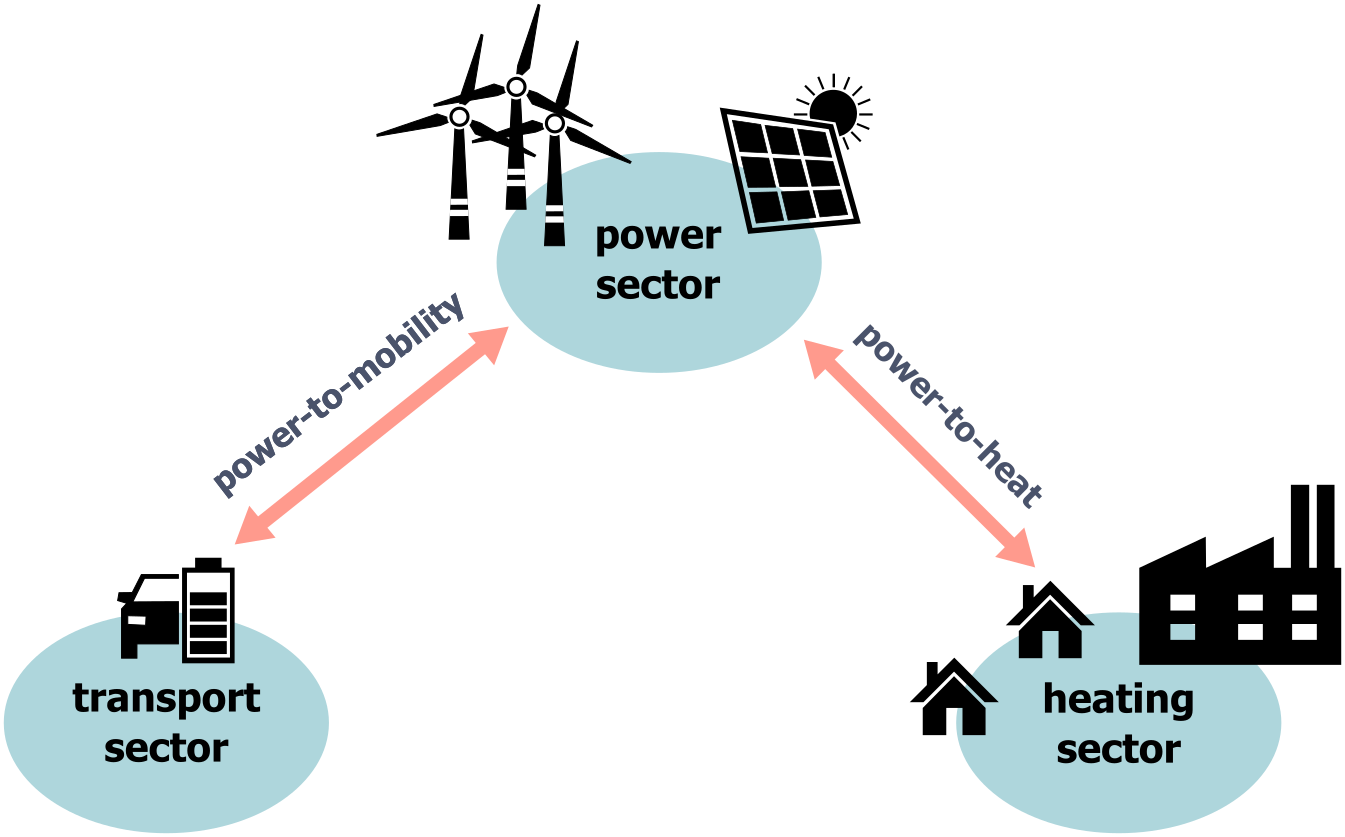
The coupling of energy sectors includes the storage or transformation to another energy carrier (like hydrogen) of superfluous electrical energy, as well the layout and operation of energy transportation networks, see e.g. [43, 61, 185].
On the mathematical/computational side, challenges arise because mathematical models of different energy conversion processes and energy transport networks live on very different time scales such as e.g., gas transport networks or electrical power networks. Furthermore, while most energy transport networks are currently operated in a stationary regime, in the future dynamic approaches are required that allow control and optimization of energy production and transport in real time, see e.g. [34, 152]. These further challenges lead to the following model class wish-list for a new flexible modeling, simulation, optimization, and control framework.
-
•
The model class should allow for automated modeling, in a modularized, and network based fashion, including pure data-based models.
-
•
The mathematical representation should allow coupling of mathematical models across different scales and physical domains, in continuous and discrete time.
-
•
The mathematical models should be close to the real (open or closed) physical system and easily extendable if further effects have to be considered.
-
•
The model class should have nice algebraic, geometric, and analytical properties. The models should be easy to analyze concerning existence, uniqueness, robustness, stability, uncertainty, perturbation theory, and error analysis.
-
•
The class should be invariant under local variable (coordinate) transformations (in space and time) to understand the local behavior, e.g. via local normal forms.
-
•
The model class should allow for simple space and time discretization and model reduction methods as well as fast solvers for the resulting linear and nonlinear systems of equations.
-
•
The model class should be feasible for simulation, control, optimization and data assimilation.
Can there be such a Jack of all trades? The main goal of this paper is to show that, even though many aspects are still under investigation, energy-based modeling via the model class of dissipative port-Hamiltonian (pH) descriptor systems has many great features and comes very close to being such a model class. Let us emphasize that the field of pHDAE systems is a highly active research area and many developments are just taking place. In this survey we thus focus only on selected topics.
Structure of the manuscript
The paper is organized as follows. We first review general nonlinear descriptor systems and its solution theory in Section 2 and associated control theoretical results in Section 3. Dissipative port-Hamiltonian (pH) descriptor systems are introduced in Section 4 and illustrated with several examples from different application domains in Section 5. In Section 6 we start to analyze pH descriptor systems in terms of our model class wish-list by discussing the inherent properties of pH descriptor systems. Condensed forms are presented in Section 7. We then turn to structure-preserving model order reduction in Section 8 and discuss time-discretization and associated linear system solves in Section 9. We conclude our presentation with a discussion of control methods in Section 10 and a summary (including open problems and future work) in Section 11. We emphasize that within this manuscript, we mainly focus on finite-dimensional problems. Nevertheless, the pH model class can be extended to the infinite-dimensional setting, and we provide a brief discussion and an (incomplete) list of references at the end of Section 11.
Notation
The sets , , , and denote the natural numbers, non-negative integers, real numbers, and complex numbers, respectively. For a complex number we denote its real part as . The set of matrices with values in a field is denoted with . The symbol is used for the identity matrix, whose dimension is clear from the context. The rank and corank of a matrix are denoted by and , where the latter is defined as
| (1.1) |
The transpose of a matrix and the conjugate transpose (if ) are denoted by and , respectively. To indicate that a matrix is positive definite, or positive semi-definite, we write and , respectively. The Moore-Penrose inverse of a matrix , i.e. the unique matrix satisfying , , , and , is denoted by . A block diagonal matrix with diagonal blocks is denoted by , and the span of a list of vectors is denoted by .
The spaces of continuous and -times continuously differentiable functions (with ) from the time interval to some Banach space are denoted by and , respectively. For a function we write to denote the (time) derivative. Similarly, we use the notation for the second derivative and for the th derivative. The Jacobian of a function is denoted by .
Abbreviations
Throughout the manuscript, we use the following abbreviations.
| DAE | differential-algebraic equation |
|---|---|
| dHDAE | dissipative Hamiltonian differential-algebraic equation |
| ECRM | effort constraint reduction method |
| FCRM | flow constraint reduction method |
| IRKA | iterative rational Krylov algorithm |
| LTI | linear time-invariant |
| LTV | linear time-varying |
| MM | moment matching |
| MSO | modeling, simulation, and optimization |
| MOR | model order reduction |
| ODE | ordinary differential equation |
| PDE | partial differential equation |
| pH | port-Hamiltonian |
| pHODE | port-Hamiltonian ordinary differential equation |
| pHDAE | port-Hamiltonian differential-algebraic equation |
| ROM | reduced order model |
2. The model class of descriptor systems
To allow network-based automated modularized modeling via interconnection, constraint-preserving simulation, optimization, and control of dynamic models, it is common practice in many application domains to use the class of (implicit) control systems, called descriptor systems or differential-algebraic equation (DAE) systems, of the form
| (2.1a) | ||||
| (2.1b) | ||||
on some time interval with
with open domains, vector spaces, or manifolds . In the finite dimensional case of real systems, which is predominantly discussed in this paper, we assume for the ease of presentation that
We refer to , , and , as the state, input, and output, respectively.
Note that there can be very different roles of inputs in different applications, e.g., to deal with control actions, interconnections, or disturbances, and different roles of outputs e.g., for measurements, interconnection, or observer design. Also, the models typically have parameters and/or may have random uncertain components such as e.g., unmodeled quantities, uncertainty in parameters, or disturbances.
We remark that most of the results and methods we present also hold for complex systems, but we restrict ourselves to the real case in this survey. In the following, for the sake of a simpler presentation, we will also often omit the time- or space argument whenever this is appropriate or clear from the context.
2.1. Solution concept
It is clear that depending on the application, different solution concepts for (2.1) may be necessary, see e.g. [41, 126, 138].
In the finite dimensional setting we restrict ourselves to classical function spaces of continuous or continuously differentiable functions. For control problems as in (2.1) we often follow the behavior framework, see for instance [174], in which a new combined state vector
| (2.2) |
is introduced (or if only the state-equation (2.1a) is considered). The descriptor system (2.1) is then turned into an under-determined DAE, see for instance [125], i.e., the meaning of the variables is not distinguished any more.
Definition 2.1 (Solution concept).
Let us emphasize that for DAE systems, typically, not every initial value is consistent. This is due to the fact that in order to deal with algebraic constraints as well as over- and under-determined systems, we allow the Jacobian to be singular or even rectangular. We refer to the forthcoming Section 2.2 for further details. For inconsistent initial values and systems with jumps in the coefficients one may still obtain a solution using weaker solution concepts, see e.g. [126, 182, 183, 218]. However, for ease of presentation, we will not cover these weaker solution concepts in this survey.
2.2. Solution theory for general nonlinear descriptor systems
In this subsection we recall the solution theory for general DAE systems
| (2.4) |
with and open sets . Here is the standard state or an extended behavior vector as in (2.2).
If the Jacobian is not square or singular, then a solution of (2.4), provided such a solution exists, may depend on derivatives of . This is illustrated in the following example.
Example 2.2.
Consider a linear DAE of the form
| (2.5) |
We immediately notice that does not contribute to the equations and hence can be chosen arbitrarily. Moreover, the third equation dictates , thus detailing that a smooth function is not sufficient for a solution to exist. The second equation yields , and hence the only valid initial value for is determined by . Substituting into the first equation yields
| (2.6) |
showing that the solution depends on the derivative of . Moreover, we notice that (2.6) constitutes another algebraic equation that is implicitly encoded in (2.5).
The difficulties arising with these differentations are classified by so-called index concepts, see [160] for a survey. In this paper, we mainly make use of the strangeness index concept [126], which is, roughly speaking, a generalization of the differentiation index, cf. [41], to under- and overdetermined systems. The strangeness index is based on the derivative array of level , see [52], defined as
| (2.7) |
Since it is a-priori not clear, that the DAE (2.4) is solvable and that the dimension of the solution manifold in terms of the algebraic vaiables is invariant over time, we need to assume that the set
| (2.8) |
is nonempty and (locally) forms a manifold. For notational convenience we assume that is a manifold of dimension . The number will later correspond to the dimension of the regular part of the DAE. Following [124], we introduce the Jacobians
| (2.9a) | ||||
| (2.9b) | ||||
In the following, we will make some constant rank assumptions, which in turn is the basis for a (local) smooth full rank decomposition as provided in the next theorem, see [126, Thm. 4.3].
Theorem 2.3.
For open sets let . Furthermore, assume that for all . Then, for every there exists a sufficiently small neighborhood of , and matrix functions and with pointwise orthonormal columns such that
To analyze the nonlinear DAE (2.4) we now make the following assumption, taken from [125] and presented similarly as in [221], to filter out the regular part. Note that we use the terminology to denote the difference between the size of a matrix and its rank; see also (1.1) for a formal definition.
Assumption 2.4.
The quantity in 2.4 measures the number of equations in the original system that give rise to trivial equations , i.e., it counts the number of redundancies in the system. After the quantification of the regular and redundant parts of the DAE (2.4), we use the next assumption to filter out the algebraic equations.
Assumption 2.5.
2.5 together with Theorem 2.3 ensures (locally) the existence of a smooth matrix function with pointwise maximal rank on that satisfies
| (2.13) |
The (linearized) algebraic equations are thus encoded in the matrix function
| (2.14) |
To ensure that we are able to solve the algebraic equations for unknowns, requires the matrix in (2.14) to have full rank. This is indeed the case, since (2.13) together with 2.4 implies that
Again, Theorem 2.3 implies (locally) the existence of a smooth matrix function
with pointwise maximal rank satisfying
| (2.15) |
The remaining differential equations must be contained in the original DAE (2.4) (in contrast to the algebraic equations, which are contained in the derivative array), and thus, we make the following additional assumption.
Assumption 2.6.
Once again, we employ Theorem 2.3 to (locally) obtain a smooth matrix function of size with pointwise maximal rank that satisfies . The matrix function will later be used to filter out the differential equations.
To summarize the previous discussion, we make the following assumption, which for historical reasons (cf. [125]) and since in the linear case it is actually a theorem, is referred to as a hypothesis. Note that due to the local character of Theorem 2.3 all assumptions hold only in a suitable neighborhood.
Hypothesis 2.7.
There exists integers , , , and such that defined in (2.8) is nonempty and such that for every there exists a (sufficiently small) neighborhood in which the following properties hold:
-
(i)
The set forms a manifold of dimension .
-
(ii)
We have on .
-
(iii)
We have on (with the convention ).
-
(iv)
We have on , such that there exist smooth matrix functions and of size and , respectively, and pointwise maximal rank, satisfying , , and on .
-
(v)
We have on such that there exists a smooth matrix function of size and pointwise maximal rank, satisfying .
Definition 2.8.
Remark 2.9.
Following the discussion in [125], we can use the matrix functions and to construct the DAE
| (2.16) |
with
Note, that although the matrix functions and depend on derivatives of , it is possible to show (cf. [125]) that the reduced quantities and are independent of higher derivatives of . In addition, one can show that (2.16) satisfies 2.7 with characteristic values , , , and . In particular, (2.16) is strangeness-free.
Hypothesis 2.10.
There exist integers and such that the set defined in (2.8) is nonempty and such that for every there exists a (sufficiently small) neighborhood in which the following properties hold:
-
(i)
We have on such that there exists a smooth matrix function of size and pointwise maximal rank such that on .
-
(ii)
We have on such that there exists a smooth matrix function of size with and pointwise maximal rank, satisfying on .
-
(iii)
We have on such that there exists a smooth matrix function of size and pointwise maximal rank, satisfying .
The relation between the original DAE (2.4) and the strangeness-free reformulation (2.16) is given in the following theorem, taken from [126, Thm. 4.11 and Thm. 4.13]. For the ease of presentation, we focus here on the regular case using 2.10 and remark that a similar result is also available for the more general setting described in 2.7, see [125] for further details.
Theorem 2.11.
Remark 2.12.
The relation of the strangeness index concept as presented above to other index concepts commonly used in the theory of DAEs, such as the differentiation index [53], the perturbation index [104], the tractability index [138], the geometric index [194, 189], and the structural index [172, 178], is discussed in [160].
2.3. Linear time-varying DAE systems
If the DAE (2.4) is linear time-varying, i.e., of the form
| (2.17) |
with smooth matrix functions , then the analysis of the previous subsection can be further simplified. In this case, the Jacobians (2.9) are given as
Since these matrix functions do not depend on the state variable nor its derivatives, we can get rid of the local character of 2.7 (respectively 2.10) by using the following simplified version of the smooth rank-revealing decomposition (cf. Theorem 2.3), see for instance [126, Thm. 3.9].
Theorem 2.13.
Let , , with for all . Then there exist pointwise orthogonal functions and , such that
with pointwise nonsingular .
In general, we can now proceed as in 2.7 and construct the matrix functions and . To avoid checking that is nonempty, we further construct a matrix function of size with pointwise maximal rank that filters out equations that do not depend on and its derivatives. If this number of equations is nonzero, we check whether the right-hand side vanishes as well. If this is the case, then we omit these equations. If not, then and the problem has to be regularized [126]. Defining
and
we obtain the solution equivalent strangeness-free system
| (2.18) |
Remark 2.14.
In the behavior case for a control system, where the state variable is given as , the matrix functions and have a block column structure, where the second block column corresponds to the control. Since the constructed coefficients and are obtained by transformations of the derivative array from the left, the block column structure of is retained in these matrices. Moreover, the strangeness-free reformulation does not depend on derivatives of the control .
If we further allow transformations of the solution space via a pointwise nonsingular matrix function, then we can obtain the following solvability result for the DAE (2.17).
Theorem 2.15.
Under some constant rank assumptions the DAE (2.17) is equivalent, in the sense that there is a change of basis in the solution space via a pointwise nonsingular matrix function, to a DAE of the form
where and are determined from .
-
(i)
If , then (2.17) is solvable if and only if .
-
(ii)
An initial value is consistent if and only if in addition the condition is implied by the initial condition.
-
(iii)
The initial value problem is uniquely solvable if and only if in addition .
2.4. Linear time-invariant DAE systems
In principle, we can perform the analysis for the linear time-varying case also in the case of general constant coefficient linear DAE systems
| (2.19) |
with matrices , also referred to linear time-invariant (LTI) DAE systems. However, in this setting it is common to work with an equivalence transformation and a corresponding canonical form. For notational convenience, for the next result we also allow complex valued matrices in (2.19) and work in the field of complex numbers.
We call the matrix pencils with , (strongly) equivalent, if there exists nonsingular matrices and such that
In this case, we write . The associated canonical form is given by the Kronecker canonical form, see e.g. [82].
Theorem 2.16 (Kronecker canonical form).
Let . Then
where the block entries have the following properties:
-
(i)
Every entry is a bidiagonal block of size , , of the form
-
(ii)
Every entry is a bidiagonal block of size , , of the form
-
(iii)
Every entry is a Jordan block of size , , , of the form
-
(iv)
Every entry is a nilpotent block of size , , of the form
The Kronecker canonical form is unique up to permutation of the blocks.
Remark 2.17.
If the matrices are real-valued and we want to stay within the field of real numbers, then only real-valued transformation matrices may be used. The corresponding canonical form is called the real Kronecker canonical form. Here, the blocks with are in real Jordan canonical form instead, but the other blocks are as in the complex case.
A value is called (finite) eigenvalue of if
If zero is an eigenvalue of , then is said to be an eigenvalue of . The blocks correspond to finite eigenvalues and the blocks to the eigenvalue . The size of the largest block is called the (Kronecker) index of the pencil , where, by convention, if is invertible. A finite eigenvalue is called semisimple if the largest Jordan block associated with this block has . The pencil is called regular if and for some . For regular pencils the Kronecker canonical form simplifies to the Weierstraß canonical form.
Theorem 2.18 (Weierstraß canonical form).
Assume that the pencil with matrices ( is regular. Then
| (2.20) |
where and are in Jordan (real Jordan) canonical form and is nilpotent.
If the pencil is not regular then there may not exist a solution of (2.19) or it may not be unique, see for instance Example 2.2, while in the regular case one has the following theorem, see [126] for the complex case.
Theorem 2.19.
Consider a regular matrix pencil of real square matrices and let and be nonsingular matrices which transform (2.19) to its real Weierstraß canonical form (2.20), i.e.
where are in real Jordan canonical form and is nilpotent of nilpotency index . Set
with analogous partitioning. If , then the DAE (2.19) is solvable. An initial value is consistent if and only if
In particular, the set of consistent initial values is nonempty and every initial value problem with consistent initial condition is uniquely solvable.
Remark 2.20.
To clarify the difference between the (Kronecker) index and the strangeness index, observe that a regular LTI DAE system has (Kronecker) index , then its strangeness index is and if , then also , see also [160].
3. Control concepts for general DAE systems
In this section we discuss different aspects related to control theory of general DAE systems. Most of our discussion focuses on linear descriptor systems of the form
| (3.1a) | ||||
| (3.1b) | ||||
with either
-
–
matrices , , for the LTI case, and
-
–
matrix functions , , for the linear time-varying (LTV) case.
Remark 3.1.
In general, the descriptor system (3.1) may also include a feedthrough term, i.e., the output equation (3.1b) is given as
with a suitable matrix or matrix function . However, in the DAE context, we can rewrite the descriptor system (3.1) without the feedthrough term, as follows. Consider any decomposition and the extended system matrices or matrix functions,
Then the solution of the associated descriptor system contains as a part the solution of the descriptor system with feedthrough term.
3.1. Feedback regularization
As we have seen in Section 2, a DAE system may not be regular, i.e., there may not be any initial values such that the initial value problem has a solution, or a solution for a consistent initial value may not be unique. To deal with this situation, we first discuss how to regularize a descriptor system via instantaneous, proportional (linear) state or output feedback, i.e., via feedback laws of the form
| (3.2) |
respectively, with suitable matrices or matrix functions and . After applying such a feedback, the closed-loop system matrices, respectively matrix functions, are given as and
respectively.
We start our analysis for the LTI case and recall important conditions for controllability and observability. If the matrix in (3.1) is nonsingular, then the well-known Hautus lemma, see e.g. [62], asserts that the LTI descriptor system (3.1) is controllable if and only if
| (3.3) |
If is singular, then the situation is more involved and we need the following conditions, taken for instance from [62, 47].
Definition 3.2.
The corresponding dual conditions with respect to the output equation are given as
| (3.5) | ||||
| (3.6) |
respectively, where is a matrix that spans the kernel of .
Definition 3.3.
Consider the LTI descriptor system (3.1) and let be a matrix with columns that span the kernel of .
- (i)
- (ii)
- (iii)
Conditions (3.5) and (3.6) are preserved under non-singular equivalence transformations as well as under state and output feedback. More precisely, if the system satisfies (3.5) and (3.6), then for any non-singular , , and any and , the system with coefficients satisfies the same condition for all of the following three choices:
Analogous invariance properties hold for (3.5) and (3.6). Further details and properties of LTI DAE systems are discussed in [33].
Note, however, that regularity or non-regularity of the pencil and the (Kronecker) index are in general not preserved under state or output feedback, respectively. On the contrary, feedback of the form (3.2) may be used to regularize the system, as detailed in the following theorem taken from [47].
Theorem 3.4.
Consider the LTI descriptor system (3.1).
- (i)
- (ii)
Remark 3.5.
Although instantaneous feedback is a convenient theoretical approach, it may suffer from the fact that signals have to be measured first, and some calculations have to be carried out, thus resulting in an intrinsically necessary time delay. If this time delay cannot be ignored in the modeling phase, then for some , the feedback takes the form
thus rendering the closed-loop system a delay DAE. However, the DAE can be regularized with delayed feedback if and only if it can be regularized with instantaneous feedback, see [219, 221] for further details. Nevertheless, we always assume that the feedback delay can be ignored in the modeling phase within this survey.
For the feedback regularization in the LTV and nonlinear case, we follow [54], and use the behavior approach as introduced in (2.2). In more detail, for the LTV descriptor system (3.1), we form the (matrix) functions
| (3.7) |
Ignoring the fact that is composed of parts that may have quite different orders of differentiability, we form the derivative array (2.7) and follow the approach presented in Section 2.3. In more detail, we construct matrices , , and , such that the system
| (3.8) |
is solution equivalent to (3.1) and strangeness-free. Since the matrix functions are obtained solely by transformations of the derivative array from the left, the partitioning of the matrices as introduced in (3.7) is retained in (3.8), see also Remark 2.14. In particular, the state and the input function are not mixed, such that we can rewrite (3.8) as
| (3.9) |
with , , and .
Remark 3.6.
Note that we have constructed (3.8) such that the system is strangeness-free (with respect to the combined state variable ). Since (3.9) is simply obtained by rewriting (3.8), it is also strangeness-free with respect to . However, it may not be strangeness-free with respect to the original state variable (in the sense that we assume to be given). To distinguish this subtlety in the following, we say that a descriptor system is strangeness-free as a free system, if it is strangeness-free with respect to for given input .
To theoretically analyze the regularizability via feedback control, we use the following condensed form, see [132].
Theorem 3.7.
Consider the LTV descriptor system (3.1) and assume that the corresponding behavior system defined in (3.7) has a well-defined strangeness index with strangeness-free form (3.8). Then, under some constant rank assumptions, there exist pointwise nonsingular matrix functions , , , , such that setting
and multiplying (3.9) by appropriate matrix functions from the left, yields a transformed control system of the form
| (3.10a) | |||||
| (3.10b) | |||||
| (3.10c) | |||||
| (3.10d) | |||||
| (3.10e) | |||||
| (3.10f) | |||||
where the number at the end of each block equation denotes the number of equations within this block.
Corollary 3.8.
Let the assumptions be as in Theorem 3.7. Furthermore, let the quantities and defined in (3.10) be constant. Then the following properties hold.
- (i)
-
(ii)
If , then for a given input function , an initial value is consistent if and only if it implies (3.10b). Solutions of the corresponding initial value problem will in general not be unique.
-
(iii)
The system is regular and strangeness-free (as a free system) if and only if and .
Analogous to the constant coefficient case we can use proportial feedback to modify some of the system properties. However, the following result, see [126, Thm. 3.80], states that some properties stay invariant.
Theorem 3.9.
Consider the LTV descriptor system (3.1) and suppose that the assumptions of Theorem 3.7 are satisfied. Then, the characteristic values , , and are invariant under proportional state feedback and proportional output feedback.
The strangeness index (as a free system) as well as the regularity of the system can, however, be modified by proportional feedback, cf. [132].
Corollary 3.10.
Let the assumptions of Corollary 3.8 hold.
-
(i)
There exists a state feedback such that the closed-loop system
is regular (as a free system) if and only if and .
-
(ii)
There exists an output feedback such that the closed-loop system
is regular (as a free system) if and only if , , and .
3.2. Stability
One of the key questions in control is whether a system can be stabilized via feedback control. In this section we therefore recall the stability theory for ordinary differential equations (ODEs) and discuss how these concepts are generalized to DAE systems. The classical stability concepts for ODEs are as follows, see, e.g., [109]. Consider an ODE of the form
| (3.11) |
and denote the solution satisfying the initial condition by .
Definition 3.11.
A solution of (3.11) is called
-
(i)
stable if for every there exists such that for all with
-
–
the initial value problem (3.11) with initial condition is solvable on and
-
–
the solution satisfies on ;
-
–
-
(ii)
asymptotically stable if it is stable and there exists such that for all with
-
–
the initial value problem (3.11) with initial condition is solvable on and
-
–
the solution satisfies ;
-
–
-
(iii)
exponentially stable if it is stable and exponentially attractive, i.e., if there exist , , and such that for all with
-
–
the initial value problem (3.11) with initial condition is solvable on and
-
–
the solution satisfies the estimate
If does not depend on , then we say the solution is uniformly (exponentially) stable.
-
–
By shifting the arguments we may assume that the reference solution is the trivial solution .
Remark 3.12.
For DAE systems
the stability concepts in Definition 3.11 essentially carry over. However, when perturbing a consistent initial value, it may happen that the perturbed initial value is not consistent anymore. Then the solution (if one allows discontinuities in the part of the state vector that is not differentiated) has a discontinuous jump that transfers the solution to the constraint manifold. For a strangeness-free DAE this would not be a problem because such a jump does not destroy the stability properties. If, however, the strangeness index is bigger than zero then, due to the required differentiations, the solution may only exist in the distributional sense, see for instance [126, 182, 218].
Example 3.13.
Consider the homogeneous linear time-invariant DAE from [67],
If then the DAE is strangeness-free and has the solution
With a consistent initial value , the solution is asymptotically stable but this limit would not exist for except if is bounded for . If then the DAE has strangeness index one and for the solution , the initial value is restricted as well. For then exists and is the discontinuous function that jumps from to at and would only be representable by a delta distribution. Finally, if then the solution is unstable.
The stability analysis and computational methods for DAE systems, therefore, assumes uniquely solvable strangeness-free systems. If the system is not strangeness-free, then one first performs a strangeness-free reformulation as discussed in Section 2.2.
For a strangeness-free system then a solution of the system is called stable, asymptotically stable, (uniformly) exponentially stable, respectively, if it satisfies the corresponding condition in Definition 3.11. Then many analytical results and computational methods can be extended to the case of strangeness-free DAE systems, see [127, 143, 144, 147, 146].
For LTI ODE systems
| (3.12) |
with , it is well-known, see e.g. [3], that the system is asymptotically (and also uniformly exponentially) stable if all the eigenvalues are in the open left half of the complex plane and stable if all the eigenvalues are in the closed left half plane and the eigenvalues on the imaginary axis are semisimple, i.e. the associated Jordan blocks have size at most one.
The stability analysis can also be carried out via the computation of a Lyapunov function given by , where for stability is a solution of the Lyapunov inequality
| (3.13) |
and for asymptotic stability it is a positive definite solution of the strict inequality, , see, e.g., [116].
The spectral characterization of stability for ODE systems can be generalized to LTI DAE systems
| (3.14) |
with , see e.g. [67].
Theorem 3.14.
Consider the DAE (3.14) with a regular pencil of (Kronecker) index at most one. The trivial solution then has the following stability properties:
-
(i)
If all finite eigenvalues have non-positive real part and the eigenvalues on the imaginary axis are semisimple, then the trivial solution is stable.
-
(ii)
If all finite eigenvalues have negative real part, then the trivial solution is uniformly and thus exponentially and asymptotically stable.
For LTV ordinary differential-equations
| (3.15) |
the different stability properties are characterized by means of the fundamental solution that satisfies
| (3.16) |
such that , see e.g. [3].
Theorem 3.15.
To obtain the results that extend this characterization to LTV DAE systems
| (3.17) |
assume again that the initial value problem associated with (3.17) has a unique solution for every consistent initial value and is strangeness-free. If the system is not strangeness-free then one first performs the transformation to strangeness-free form as in Section 2.2.
For a regular strangeness-free system (3.17) there exist pointwise orthogonal matrix functions , such that
| (3.18) |
with pointwise nonsingular, and . Under the condition of a bounded matrix function , one obtains the algebraic equation and the so-called inherent ODE associated with (3.17) given by
| (3.19) |
It is then clear that for the different stability concepts to extend to DAE systems it is necessary that (3.19) satisfies the corresponding stability conditions.
Remark 3.16.
For ODE systems there is also a well-known extension of the spectral stability analysis via the computation of Lyapunov, Bohl and Sacker-Sell spectral intervals. These results have been extended to DAE systems in [32, 143, 145, 146, 147]. We will not discuss this topic here further, but just mention that it is computationally highly expensive.
For general autonomous nonlinear ODE systems the fundamental approach to analyze the stability properties is to compute a Lyapunov function such that is negative definite in neighborhood of the solution . If such a Lyapunov function exists, then the equilibrium solution is asymptotically stable, see e.g. [136, 3]. This approach can be used as well for general strangeness-free DAE systems by reducing the system to the inherent ODE.
3.3. Stabilization
Since in physical systems the stability of a solution is typically a crucial property, it is important to know how a stable system behaves under disturbances or uncertainties in the coefficients and how an unstable system can be stabilized with the help of available feedback control. Let us consider this question first for LTI control problems of the form (3.1) and ask whether it is possible to achieve stability or asymptotic stability via proportional state or output feedback.
We have seen in Theorem 3.4 that for strongly stabilizable systems there exist an such that the pair is regular and of index at most one, and for strongly stabilizable and strongly detectable systems there exist an such that the pair is regular and of (Kronecker) index at most one. In the construction of stabilizing feedbacks we can therefore assume that such a (preliminary) state or output feedback has been performed, and therefore that the pair is regular and of (Kronecker) index at most one.
The calculation of stabilizing feedback control laws can then be performed via an optimal control approach (see also the forthcoming Section 3.5), by minimizing the cost functional
| (3.20) |
subject to the constraint (3.1). We could have also used the output function instead of the state function by inserting and modifying the weights accordingly. The following results, which are based on the Pontryagium maximum principle, are taken from [159].
Theorem 3.17.
Consider the optimal control problem to minimize (3.20) subject to the constraint (3.1) with a pair that is regular and of (Kronecker) index at most one. Suppose that a continuous solution to the optimal control problem exists and let be the solution of (3.1) with this input function. Then, there exists a Lagrange multiplier function such that , , and satisfy the boundary value problem
| (3.21) |
with boundary conditions
| (3.22) |
where denotes the Moore-Penrose inverse of .
Theorem 3.18.
The solution of the optimality boundary value problem (3.21) with boundary conditions (3.22) will yield the optimal control and the corresponding optimal state . However, in many real-world applications one would like the optimal control to be a state feedback. A sufficient condition for this to hold is that the matrix pencil associated with (3.21) is regular of (Kronecker) index at most one and has no purely imaginary eigenvalue. If the matrix is positive definite and is strongly stabilizable, then this can be guaranteed, see [159], and we can proceed as follows. Recall that we have assumed that the pair is regular and of (Kronecker) index at most one. Then the coefficients can be transformed such that is in Weierstraß canonical form (2.20), i.e.
with transformed cost function
Setting
and reordering equations and unknowns we obtain the transformed boundary value problem
| (3.23) |
with boundary conditions
| (3.24) |
Solving the third and fourth equation in (3.23) gives
Inserting these in the other equations gives the reduced optimality system
| (3.25) |
with , , and boundary conditions (3.24). This is the classical optimality condition associated with the ODE constraint and the cost matrix
for which the standard theory for optimal control with ODEs constraints can be applied, see, e.g., [159].
With an ansatz with the optimal control takes the form of a state feedback
Inserting in (3.25) we obtain the system
A sufficient condition for this system to have a solution is, see [159], that we can find a positive semi-definite solution to the algebraic Riccati equation
If is not invertible then there are further restrictions on the boundary conditions that may defer the solvability of the boundary value problem, see [159] for details and the forthcoming Section 10.2.
3.4. Passivity
Another important property of control systems is the concept of passivity. Let us first introduce a passivity definition for general DAE control systems of the form (2.1) with a state space , input space , and output space . See [51] for the definition for ODE systems.
To introduce this definition we consider a positive definite and quadratic storage function as well as a supply function satisfying
Definition 3.19.
An autonomous DAE of the from (2.1) is called (strictly) passive with respect to the storage function and the supply function if there exists a positive semi-definite (positive definite) function , such that for any and for any the equation
| (3.26) |
holds for all .
Equation (3.26) is called storage energy balance equation and directly implies that the dissipation inequality
holds for all .
For LTI ODE systems of the form
passivity can be characterized, see [230], via the existence of a positive definite solution of a linear matrix inequality, the Kalman–Yakubovich–Popov inequality
| (3.27) |
For strict passivity this inequality has to be strict. Note that (3.27) generalizes the Lyapunov inequality (3.13), which is just the leading block, and hence (strict) passivity directly implies (asymptotic) stability.
The relationship between passivity and the linear matrix inequality (3.27) has been extended to LTI DAE systems in [190, 193].
Since passive systems are closely related to port-Hamiltonian systems, we will come back to this topic in Section 7.6.
3.5. Optimal control
An important task in control theory is the solution of optimal control problems that minimize a cost functional subject to an ODE or DAE system. The optimal control theory for general nonlinear DAE systems was presented in [128]. In this section we recall these general results.
Consider the optimal control problem to minimize a cost functional
subject to a constraint given by an initial value problem associated with a nonlinear DAE system
We can rewrite this problem in the behavior representation, see the discussion in Section 2.2, with , and then study the optimization problem
| (3.28) |
subject to the constraint
| (3.29) |
If 2.7 holds, then for this system we (locally via the implicit function theorem) have a strangeness-free reformulation, cf. [126], as
| (3.30) | ||||
and the associated cost function reads
| (3.31) |
For this formulation, the necessary optimality conditions in the space
are presented in the following theorem. We refer to [128] for the original presentation and the proof.
Theorem 3.20.
Theorem 3.20 is a local result based on the implicit function theorem that has to be modified to turn it into a computationally feasible procedure, cf. [128], and which can be substantially strengthened for the minimization of quadratic cost functionals
| (3.32) |
with matrix functions , , , and , subject to LTV DAE constraints
| (3.33) |
with , , , , , , and . Using the property that for the Moore-Penrose inverse of , we have
we interpret (3.33) as
This allows the particular solution space, see [123],
which takes care that the differentiability of the state variable is only required in this restricted space. Note that with this definition, we slightly extend our solution concept from Definition 2.1.
Using this solution space, in [128] the following necessary optimality condition was derived.
Theorem 3.21.
Consider the optimal control problem (3.32) subject to (3.33) with a consistent initial condition. Suppose that (3.33) is strangeness-free as a behavior system and that the range of is contained in the of . If is a solution to this optimal control problem, then there exists a Lagrange multiplier function , such that satisfy the boundary value problem
| (3.34a) | ||||
| (3.34b) | ||||
| (3.34c) | ||||
| (3.34d) | ||||
Remark 3.22.
If we have an output equation, then we can also consider the cost functional (3.32) with the state replaced by the output. This problem can be treated analogously by inserting the output equation in the cost functional and renaming the coefficients. The same approach with a modified cost functional can also be used for the case that we want to optimally drive the solution to a reference function .
It [129], see also [17, 134], it was demonstrated that it is in general not possible to drop the assumptions of Theorem 3.21 and instead consider the formal optimality system
| (3.35) | ||||||
However, if this formal optimality system has a unique solution, then the state and the control are correct but the optimal Lagrange multiplier may be different. In this case, under some further assumptions, also a sufficient condition has been shown in [129] generalizing results from [17].
Theorem 3.23.
Consider the optimal control problem (3.32) subject to (3.33) with a consistent initial condition and suppose that in the cost functional (3.32) we have that the matrix functions and are (pointwise) positive semi-definite. If satisfies the formal optimality system (3.35), then for any satisfying (3.33) we have
Numerically, the solution of the boundary value problem (which always is DAE) is a challenge, in particular for large-scale problems. For the case that and if is positive definite, which means that the optimality system is strangeness-free, then a classical approach that is successfully employed in many applications is to resolve (3.34c) for , and then to decouple the state equation (3.34a) and the adjoint equation (3.34b) via the solution of a Riccati differential equation.
If some further conditions hold, then the Riccati approach can also be carried out for DAE systems, see [129]. If the constraint system with is regular, strangeness-free, and has constant rank, then, using Theorem 2.3, there exist pointwise orthogonal and such that
| (3.36) |
with and pointwise nonsingular. Forming the formal optimality system associated with this transformed system and rearranging the equations, the following theorem is proved in [129].
Theorem 3.24.
If is pointwise nonsingular, then
The remaining equations can be written as
Defining
we obtain the boundary value problem
| (3.37a) | ||||||
| (3.37b) | ||||||
Making the ansatz , one can solve the two initial value problems
and
to obtain and and to decouple the solution of (3.37). In [129], a Riccati approach is also obtained directly for the original optimality system (3.34) by the modified ansatz
| (3.38) | ||||
where
to fit to the solution spaces for and . If is invertible, then introducing the notation
yields two initial value problems for the Riccati DAE
| (3.39) | ||||
and
For this to be solvable, we must have with suitable and with suitable .
The major advantage of the ansatz via Riccati equations is that the resulting control can be directly expressed as a feedback control, e.g. using (3.38), we get
A similar result is also obtained if the cost functional is formulated in terms of the output and using an output feedback.
Note that in the LTI DAE case further results have been obtained, that allow the use of efficient numerical techniques for the computation of the solutions to (3.39) via eigenvalue methods, see [159].
In this section we have recalled several properties for general descriptor systems. In the following section we study the special class of port-Hamiltonian descriptor systems and show that the structure of the systems ensures many improved properties.
4. Port-Hamiltonian descriptor systems
To fulfill as many points on our wish-list as possible, we will not use general descriptor systems, but energy-based modeling within the class of (dissipative) port-Hamiltonian (pH) systems and their generalization to descriptor systems.
4.1. Nonlinear (dissipative) port-Hamiltonian descriptor systems
We start our exposition by introducing the general model class of (dissipative) pH descriptor systems, or pH differential-algebraic equation (pHDAE) systems, introduced in [162].
Definition 4.1 (pH descriptor system, pHDAE).
Consider a time interval , a state space , and an extended space . Then a (dissipative) port-Hamiltonian descriptor system (pHDAE) is a descriptor system of the form
| (4.1a) | ||||
| (4.1b) | ||||
with state , input , output , where
and an associated function , called the Hamiltonian of (4.1). Furthermore, the following properties must hold:
-
(i)
The matrix functions
(4.2a) (4.2b) called the structure matrix and dissipation matrix, respectively, satisfy and in .
- (ii)
If the pH descriptor system has no inputs and outputs, i.e., if and the output equation is omitted, then we refer to (4.1) as (dissipative) Hamiltonian differential-algebraic equation (dHDAE).
Note that in the literature and also in this survey the adjective dissipative is typically omitted, and we follow this tradition, even if the system has a dissipative part .
Remark 4.2.
Remark 4.3.
For many properties of pHDAEs that we discuss later, it is sufficient to require the properties (4.2) and (4.3) in Definition 4.1 to hold only along any solution of (4.1), thus further extending the model class. Nevertheless, to simplify the presentation, we work with the definition as presented here.
Remark 4.4.
If is the identity matrix, , and the coefficients do not explicitly depend on time , then Definition 4.1 reduces to the well-known classical representation for ODE pH systems, called pHODEs in the following, as for instance presented in [224].
Remark 4.5.
In the literature, pH systems are often described via a Dirac structure; see [224] and this approach has also been extended to descriptor systems, see [162, 223, 225], and the forthcoming Section 6.3. In this survey, however, we mostly focus on the dynamical systems point of view, which is prevalent in the simulation and control context.
In many applications, additional properties of the Hamiltonian such as convexity or non-negativity, may further strengthen the properties of pHDAEs, see Section 6. We thus make the following definition.
Definition 4.6.
The Hamiltonian for a pHDAE of the form (4.1) is called non-negative, if
Although satisfied in many applications, it may seem artificial from a mathematical point of view to require the Hamiltonian to be non-negative. This is however not a restriction, since any Hamiltonian that is bounded from below can be recast as a non-negative Hamiltonian by adding its infimum along any behavior solution. In the following we therefore always assume that the Hamiltonian is non-negative.
Remark 4.7.
The particular structure of the ports with equal dimensions and the described structure ensure that inputs and outputs are co-located or power-conjugated. This enables for easy power-conserving interconnection of pHDAE systems, see the forthcoming Section 6.4. However, in many applications, one has specific quantities that one can observe and others that one can use for control, and these are not necessarily co-located or power-conjugated. To allow classical control techniques as well as interconnectability, one can extend the inputs and outputs to obtain a power-conjugated formulation. Even if these variables are not explicitly used, they typically have a physical meaning in the context of supplied energy. We will demonstrate this with examples later on, see e.g. Sections 5.2 and 5.5.
There are different generalizations of Definition 4.1 to infinite-dimensional systems, e.g. one can formulate operator pHDAE systems via semigroup theory, introduce formal Dirac structures, or follow a gradient flow approach. In the final section of this survey, we present an incomplete list of references discussing different aspects of infinite-dimensional pHDAE systems. In this survey, we focus mainly on the finite-dimensional case. We assume that a space-discretization via Galerkin projection is performed for an infinite-dimensional case. For infinite-dimensional examples, we mimic the finite-dimensional properties, which are then preserved under Galerkin projection (see the forthcoming Section 6.2). We refer to the examples in Section 5 for further details.
4.2. Linear pHDAE systems
Important special subclasses of the general class of pHDAE systems, are LTV and LTI pHDAE systems. Such a general class with a quadratic Hamiltonian was introduced in [26].
Definition 4.8 (Linear pHDAE, quadr. Hamiltonian).
A linear time-varying descriptor system of the form
| (4.5a) | ||||
| (4.5b) | ||||
with
is called a linear pHDAE with quadratic Hamiltonian
| (4.6) |
if the following properties are satisfied.
-
(i)
The differential-operator
(4.7) is skew-adjoint, i.e. we have and for all ,
-
(ii)
The matrix function
(4.8) is positive semi-definite, i.e. for all .
If the Hamiltonian is quadratic, and the coefficients are not depending explicitly on the state , then Definitions 4.1 and 4.8 are closely related. Starting from Definition 4.8 we may set
Using the skew-adjointness of in Definition 4.8 (i) we then obtain
and
Thus, if additionally is skew-symmetric, i.e. , then the Hamiltonian satisfies the requirements (4.3) from Definition 4.1. Similarly, we notice that the positive semi-definiteness of the dissipation matrix function in Definition 4.8 is slightly more general than its counterpart in Definition 4.1. On the other hand, the requirement for the matrix functions and to be continuously differentiable, is a sufficient condition to obtain a continuously differentiable Hamiltonian as required in Definition 4.1.
Another important special class is that of (LTI) pHDAE systems with quadratic Hamiltonian, which is commonly used in closed-loop and data-based control applications as well as linear stability analysis.
Definition 4.9 (LTI pHDAE, quadr. Hamiltonian).
A descriptor system of the form
| (4.9a) | ||||
| (4.9b) | ||||
with matrices , , and is called linear time invariant pHDAE with (quadratic) Hamiltonian
| (4.10) |
if the matrices
satisfy and .
Having introduced the general modeling concept of (dissipative) pH descriptor systems, we now discuss two modeling simplifications, namely removing the factor in linear pHDAE systems and removing the feedthrough term .
4.3. Removing the factor in linear pHDAE systems
In many applications (time-varying or time-invariant) one has and that is the identity matrix in Definitions 4.8 and 4.9. In this case is the Hessian of the Hamiltonian. This representation has many advantages: All the coefficients appear linearly in (4.9), which greatly simplifies the analysis and also the perturbation theory. Also in many cases this leads to a convexification of the representation, cf. [69, 80]. In the following we will show how the factor can be removed, see [26, 158].
If has pointwise full column rank in (4.5), then the state equation can be multiplied with from the left, yielding a system with the same solution set given by
Then setting , , , , and , the transformed system
is again a pHDAE, but now has and hence .
If is not of full rank then the situation is more complex. If has constant rank in , then, using a smooth full rank decomposition (Theorem 2.13), there exist pointwise orthogonal matrix functions and of the same smoothness as such that
where the block in all three block matrices is square of size and is pointwise invertible. Since , we get and , and the transformed system, with , is given by
where is of size and of size . By the pHDAE structure it then follows that and the resulting subsystem
is a pHDAE with square and nonsingular, which determines independent of . In particular, we can multiply by as discussed before.
However, for given and , the remaining DAE system for
has no apparent structure. This is not a problem, since the variable does not contribute to the Hamiltonian. Actually, further equations, as well as state, input and output variables can always be added to a pHDAE system if they do not contribute to the Hamiltonian.
Remark 4.10.
In the case that is not of full rank, even in the case of pHODE systems the solution can grow unboundedly. In [157], the Hamiltonian ODE system
with Hamiltonian is presented. It has the solution , and thus has linear growth and thus is not stable.
Here the first equation is a pHODE with Hamiltonian , while the second equation has no specific structure and does not contribute to the Hamiltonian.
Remark 4.11.
A similar approach of generating a representation without a factor for nonlinear and even infinite-dimensional evolution equations in a weak formulation has been presented in [69], where for applications in linear generalized gradient systems, it is discussed that even in the case that , it may be more convenient to use a representation that reverses the roles of and . Note that if in both and are (pointwise) invertible, then by multiplying with , and setting , , the equivalent new system
has and .
In view of the observations concerning the term , one should avoid introducing a term in the representation already on the modeling level and rather work with an in front of the derivative.
4.4. Removing the feedthrough term in linear pHDAE systems
In many pHDAE models, there is no feedthrough term and in this case, by the semi-definiteness of the dissipation matrix , also . If this is not the case, then (under some constant rank assumptions) one can always remove the feedthrough term by extending the state space. However, the simple construction presented in Remark 3.1 may destroy the pH structure. In this subsection, we, therefore, discuss how such an extension is possible while preserving the pHDAE structure.
Consider the linear time-varying or time-invariant pHDAE in (4.9), or (4.5), respectively, and assume that has constant rank. Under this assumption by Theorem 2.13 there exists a pointwise orthogonal matrix function , such that
with pointwise nonsingular. By construction, the symmetric part of is pointwise positive semi-definite. Setting, with analogous partitioning,
the system can be written as
| (4.11a) | ||||
| (4.11b) | ||||
| (4.11c) | ||||
Using the positive semi-definiteness of the matrix (function) in Definitions 4.8 and 4.9, we immediately obtain . Let us introduce the new variable to obtain the extended system
Note that by this extension the Hamiltonian and the output have not changed, they are just formulated in different variables. Then, by multiplying the state equation with the nonsingular matrix (function) from the left, we obtain the extended descriptor system
| (4.12) | ||||
with extended state and matrices
Theorem 4.12.
Proof.
It remains to show that is (pointwise) positive semi-definite. Since the positive semi-definiteness of is equivalent to the positive semi-definiteness of the symmetric part of
the claim is an immediate consequence of the positive semi-definiteness of the dissipation matrix (4.8) and the Schur complement. Note that due to the special form of the coefficient of the derivative, the changes of basis do not introduce extra derivative terms. ∎
Thus, in the following we often assume that , which then also implies . We should be aware, however, that the matrix may be ill-conditioned with respect to inversion, so from a numerical point of view the removal of the feedthrough term may be not advisable.
Remark 4.13.
The extension of the pHDAE system by algebraic equations and variables that do not contribute to the Hamiltonian is the counterpart to Remark 4.10, where equations that do not contribute to the Hamiltonian can be separated from the system.
5. Applications and examples
In this section, we illustrate the generality and wide applicability of the model class of pHDAE systems introduced in Section 4 with several examples from different application areas. For further examples we refer to [188] and the references therein.
5.1. RLC circuit
An RLC circuit can be modeled as a directed graph with incidence matrix
conveniently partitioned into components associated with resistors, capacitors, inductors, voltage sources, and current sources; see [79] for further details. Let denote the vector of voltages at the nodes (except for the ground node at which the voltage is zero). Furthermore, let , , denote the vectors of currents along the edges for the inductors, voltage sources, and current sources, respectively, while and denote the vectors of voltages across the edges for the voltage sources and current sources. Using Kirchhoff’s current and voltage law combined with the so-called branch constitutive relations yield a pHDAE (in the spirit of Definition 4.9 with , , )
and Hamiltonian
which is associated with the stored energy in the capacitors and inductors. Here, the positive definite matrices , , and are defined via the defining properties of the resistors, capacitors, and inductors. Note that in this case we have an LTI pHDAE with quadratic Hamiltonian, and no feedthrough term.
For general circuits, recently in [169] a new pHDAE formulation has been suggested, which allows, in particular, for a structural index analysis and for more efficient and structurally robust implementations than classical modified nodal analysis. Another recent development is the formulation of dynamic iteration schemes for coupled pHDAE systems and their use in circuit simulation in [100].
5.2. Power networks
A major application of pHDAE modeling arises in power network applications. Consider the following simple model of an electrical circuit in Figure 2, which is presented in [162]. In this model is an inductor, are capacitors are resistances, and a controlled voltage source. This circuit can serve as a surrogate model of a DC generator (,), connected to a load ( with a transmission line and given by ). In real-world power networks one would have a large number of generators (including wind turbines and solar panels) and loads representing customers.
With a quadratic Hamiltonian describing the energy stored in the inductor and the two capacitors
| (5.1) |
a formulation as LTI pHDAE has the form
| (5.2a) | ||||
| (5.2b) | ||||
with , , , , and ,
If the generator is shut down (i.e. ), then the system approaches an equilibrium solution for which , so that , and then .
This system can also be considered as control problem that has the control task that a consumer (represented by a resistance ) receives a fixed amount of power . This can be achieved by controlling the voltage of the generator , so that the solution converges to the values , , , , and .
5.3. Stokes and Navier-Stokes equation
A classical example of a partial differential equation which, after proper space discretization leads to a pHDAE, see e.g. [74], are the incompressible or nearly incompressible Navier-Stokes equations describing the flow of a Newtonian fluid in a domain ,
together with suitable initial and boundary conditions, see e.g. [217]. When one linearizes around a prescribed stationary vector field , then one obtains the linearized Navier-Stokes equations,
If is also constant in space then and one obtains the Oseen equations. If also the term is neglected one obtains the Stokes equation. Performing a finite element discretization in space, see for instance [140], a Galerkin projection leads to a dHDAE of the form
| (5.3) |
where is the mass matrix, , are the skew-symmetric and the symmetric part of the discretized and linearized convection-diffusion operator, is the discretized divergence operator, which we assume to be normalized so that it is of full row rank, and is a stabilization term, typically of small norm, that is needed for some finite element spaces, see e.g. [186]. The variables and denote the discretized velocity and pressure, respectively, and is a forcing or control term.
This becomes a pHDAE by adding an output equation and an appropriate Hamiltonian, see [8]. Other possible inputs and outputs that are not necessarily co-located can be chosen, e.g. by different boundary conditions (added to the system via the trace operator and suitable Lagrange multipliers) or measurement points for the velocities or pressures.
5.4. Multiple-network poroelasticity
Biot’s poroelasticity model for quasi-static deformation, [35], describes porous materials fully saturated by a viscous fluid. Typical applications include geomechanics [236], and biomedicine [213]. The effect of different fluid compartments can be accounted for with the theory of multiple-network poroelasticity [18]. For instance, in the investigation of cerebral edema, see [220], one distinguishes different blood cycles (arterial, arteriole/capillary, venous) and a cerebrospinal fluid, giving a total of fluid compartments. The complete model is given by a coupled system of (nonlinear) partial differential equations (PDEs)
| (5.4a) | ||||
| (5.4b) | ||||
| with unknown displacements , unknown pressure variables () for the different fluid compartments, the Biot-Willis fluid-solid coupling coefficients , Biot modulus , fluid viscosities , (nonlinear) hydraulic conductivities , network transfer coefficients , volume-distributed external forces , and injection . The stress-strain relation is given by | ||||
| with the Lamé coefficients and and the identity tensor . For simplicity, we consider the system with Dirichlet boundary conditions | ||||
| (5.4c) | ||||
Following [7] (see also [72]), a pHDAE of the mixed finite-element discretization of (5.4) is given as
with positive definite mass and stiffness matrices , , and . Let us emphasize that in this representation we may use the boundary conditions as additional inputs (added to the system via the trace operator and suitable Lagrange multipliers) such that the system may be controlled via its boundary.
5.5. Pressure waves in gas network
The propagation of pressure waves on acoustic time scales through a network of gas pipelines is modeled in [42], see also [70, 71], via a linear infinite-dimensional pHDAE system on a finite directed and connected graph with vertices and edges that correspond to the pipes of the physical network. Denote by the pressure and by the mass flux in pipe , and using equations for the conservation of mass and the balance of momentum
where the coefficients , encode properties of the fluid and the pipe, and models the damping due to friction at the pipe walls. The coefficients are assumed to be positive and, for ease of presentation, constant on every pipe . To model the conservation of mass and momentum at the junctions at inner vertices of the graph, where several pipes are connected, one requires Kirchhoff’s law for the flow as well as continuity of the pressure, i.e.
Here , depending on whether the pipe starts or ends at the vertex . The time dependent quantities and denote the respective functions evaluated at the vertex . At the boundary vertices , we define co-located ports of the network by using the pressure
as input at , and the mass flux
as output. We further define initial functions
Note that typically gas is only inserted at some nodes of the network and extracted at other ends. Thus one could also use different input and output variables at the external nodes that may not necessarily be co-located. The discussed formulation however, allows easy interconnection, and still the variables have a physical interpretation.
In [70] several important properties have been shown. These include the existence of unique classical solutions for sufficiently smooth initial data , , as well as global conservation of mass, and that this system has pHDAE structure. Space-discretization via a structure-preserving mixed finite element method leads to a block-structured linear time-invariant pHDAE system
| (5.5a) | ||||
| (5.5b) | ||||
with
Here represents the discretized pressures, the discretized fluxes, while is a Lagrange multiplier vector introduced to penalize the violation of the space-discretized constraints. The coefficients , , and are positive definite, the matrix has full row rank and has full column rank. The discretized Hamiltonian is given by . Note that the Lagrange multiplier does not contribute to the Hamiltonian.
5.6. Multibody systems
Another natural class of applications arises in multibody dynamics. In [110] the model of a two-dimensional three-link mobile manipulator was derived, see also [47] for details. After linearizing around a stationary solution one obtains a control system
where is the vector of positions, is the linearized position constraint, its violation is penalized by a Lagrange multiplier vector , and is the control force applied at the actuators. The mass and stiffness matrices are positive definite and the damping matrix is positive semi-definite.
This DAE has the first and second time derivative of as hidden algebraic constraints and it is typically necessary to use a regularization procedure to make the system better suited for numerical simulation and control, see e.g. [73, 126, 181, 212]. One possibility is to replace the original constraint by its time derivative . By adding a tracking output , see e.g. [111], and transforming to first order form by introducing
one obtains a linear time-invariant pHDAE system of the form (4.9) with
The quadratic Hamiltonian (4.10) is given by
Note that the Lagrange multiplier does not contribute to the Hamiltonian.
5.7. Brake squeal
Disc brake squeal is a frequent and annoying phenomenon.
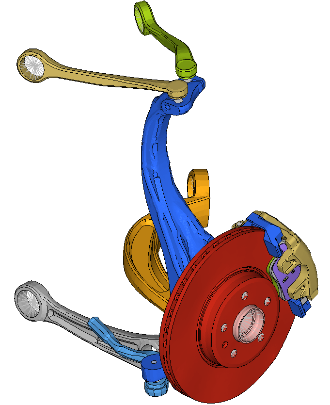
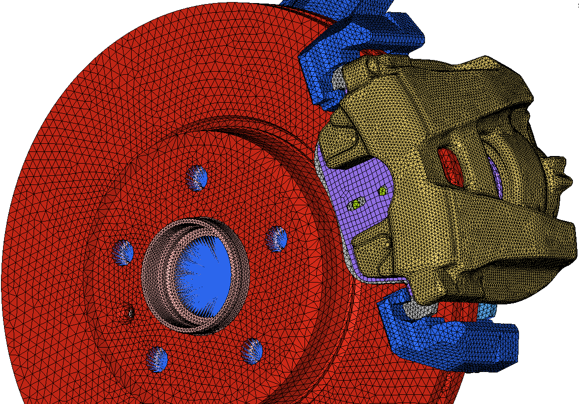
In [89] a very large finite element model of a brake system was derived that includes friction as well as circulatory and gyroscopic effects. This has the form
where is a vector of finite element coefficients, is a singular mass matrix, models material damping, models gyroscopic effects, models friction-induced damping and is typically generated from measurements, is a stiffness matrix, has no symmetry structure and models circulatory effects, while is a geometric stiffness matrix. One of many parameters is , the rotational speed of the disk scaled by a reference velocity .
Experiments indicate that there is a subcritical Hopf bifurcation (in the parameter ), when eigenvalues of the associated quadratic parametric eigenvalue problem
cross the imaginary axis. Here and are split into their symmetric and skew-symmetric parts.
By writing the system in first order formulation, it can be expressed as a perturbed dHDAE system , with
Instability and squeal arise only from the perturbation term , which is associated with the brake force restricted to the finite element nodes on the brake pad.
Performing a linear stability analysis by solving the eigenvalue problem for an industrial problem, incorporating the perturbation term via a homotopy parameter , , it has been determined in [28] that for the spectral abscissa, i.e., the maximal real part of all eigenvalues, is and for it is already , i.e., the unperturbed problem is already close to a problem with positive real part eigenvalues. The application task then is to design the brake in such a way (e.g. by including damping devices, so-called shims) that the unperturbed problem is such that the perturbation does not lead to eigenvalues in the right half plane, or at least make sure that they have a small real part.
6. Properties of pHDAE systems
In this section we discuss several general properties of the model class of pHDAE systems and show why they are a very good candidate for our modeling wishlist.
6.1. Power balance equation and dissipation inequality
A key property of pHDAE systems that shows the strong rooting in the underlying physical principles is the power balance equation and the associated dissipation inequality, see also Section 3.4.
Theorem 6.1.
Proof.
Let be a behavior solution of the pHDAE (4.1). Using the structural properties of the pHDAE system we obtain
∎
Using the fact that along any solution of (2.1), we immediately obtain that the pHDAE system satisfies the dissipation inequality
| (6.1) |
The power balance equation and the dissipation inequality are obvious in all the examples described in Section 5. In all cases the dissipation term is positive semi-definite. In the disk brake for the unforced system, without applying the brake force, cf. Section 5.7, this is also the case. The perturbation term with moves eigenvalues to the right half plane is due to the external force that can be interpreted as a supplied energy via the term .
6.2. Invariance under transformations and projection
Another essential property of the class of pHDAE systems is the invariance under different equivalence transformations, see [26, 162, 165].
Let us begin with general state space-transformations and consider and define with elements . Let and let be invertible. Define
and
together with a transformed Hamiltonian
| (6.2) |
We have the following transformation result taken from [162].
Theorem 6.2.
Proof.
The transformed DAE system is obtained from (4.1) by setting , pre-multiplying with and inserting in front of in the first equation. It is clear that if is a solution of (6.3), then is a behavior solution of the original system and if is a global diffeomorphism, then we can apply the inverse transformation to get a behavior solution for any behavior solution of the original system.
To show that (6.3) is still a pHDAE, we must check the defining conditions. By substitution, we get
since positive semi-definiteness is invariant under congruence. We also get
and
For linear pHDAE systems with quadratic Hamiltonian this invariance takes the following form, see [26].
Theorem 6.3.
Proof.
The transformed DAE system is obtained from the original DAE system by setting , pre-multiplying with , and by inserting in front of . The transformed operator corresponding to in (4.7) is given by
Because
we have that is again skew-adjoint. It is then straightforward to show that .
where is as defined in (4.8). Because is positive semi-definite for all , so is . ∎
Note that even if in an LTV pHDAE system with quadratic Hamiltonian, after the transformation given in Theorem 6.3 the extra term with will appear, and if an orthogonal change of basis is carried out in a system with then is skew-symmetric. However, even if , it has been shown in [26] that this term can be removed via a change of basis transformation that does not change the quadratic Hamiltonian.
Lemma 6.4.
Consider a pHDAE system
with Hamiltonian and . If is a pointwise invertible solution of the matrix differential equation with the initial condition , then setting and defining
then the system
is again a pHDAE with the same Hamiltonian .
Proof.
For a given matrix function , the system always has a solution that is pointwise invertible. The remainder of the proof follows by reversing the proof of Theorem 6.3 with and using that . ∎
Another important observation for linear pHDAE systems of the form (4.5) (with ) that is important in the context of space discretization and model reduction is that the pHDAE structure is invariant under Galerkin projection.
Corollary 6.5.
Remark 6.6.
Not that for LTV pHDAE systems with , strictly speaking, the invariance under Galerkin projection is violated, except if one incorporates a term between and so that the projected coefficient is approximated by .
The discussed invariance of a pHDAE system under transformations allows to simplify the representation further. These simplifications are discussed in Section 7 for linear time-varying pHDAE systems.
6.3. Geometric description of pHDAE systems
Port-Hamiltonian systems are often described through differential geometric structures known as Dirac structures, see e.g. [224]. This viewpoint is extremely helpful in many aspects, in particular in the construction of time-discretization methods, see Section 9.1.
Definition 6.7.
Let be a Euclidian vector space and its dual space. Let be a bilinear form on defined via
where is the standard duality pairing. Then a linear subspace , such that with respect to is called Dirac structure on . If , then and are called flow and effort, respectively.
The concept of a Dirac structure can also be generalized to vector bundles. Let for this denote the Whitney sum between vector bundles, see e.g. [139].
Definition 6.8.
Consider a state space and a vector bundle over with fibers . A Dirac structure over is a subbundle such that, for all , is a linear Dirac structure.
This definition generalizes the modulated Dirac structures, see [224], where is the tangent bundle to . To associate a Dirac structure to the pHDAE system (4.1), we assume that the system is autonomous, cf. Remark 4.2, and first show the following lemma.
Lemma 6.9.
Consider an autonomous pHDAE system (4.1) with skew-symmetric . If is a vector subbundle with fibers defined by
| (6.4) |
then is a Dirac structure.
Proof.
For generic and , we have
We show that if and only if for all . If , then holds for any . If , then and so there exists such that , but with . ∎
A Dirac structure for general pHDAE systems is then constructed as follows, see [162].
Theorem 6.10.
Consider an autonomous pHDAE system of the form (4.1). Define the flow fiber for all , where
Let us partition and . Then the subbundle with
is a Dirac structure over . Furthermore, the system of equations
| (6.5) | ||||||
is equivalent to the original pHDAE, and represents the power balance equation.
Proof.
Lemma 6.9 implies that is a Dirac structure. Writing (4.1) in compact form
it follows that can be written as
Together with the conditions (6.5) this is equivalent to
which is exactly the compact form of the pHDAE. Finally, note that the equation can be written as
which is the power balance equation. ∎
Note that, if we conversely want to retrieve a pHDAE system from a Dirac structure, then the additional conditions (6.5) and the definition of are needed.
Remark 6.11.
Since dHDAE systems generalize classical Hamiltonian systems, an immediate question is whether the associated flow has a geometric structure, such as symplecticity or generalized orthogonality when there is no dissipation, see [103]. While for pHODE systems this is well established, see e.g. [56, 224], for LTV dHDAE systems this has only been established recently in [204], and in a more general setting in [131].
Remark 6.12.
In the linear time-invariant case an extension that addresses different Lagrange and Dirac structures and their relation has been introduced in [225]. Ignoring the dissipation term as well as the inputs and outputs, the corresponding equation has the form
where satisfy with , i.e. the columns of , form a Lagrangian subspace, and with , i.e. the columns of are associated with a Dirac structure. A further generalization is discussed in [86].
Clearly, if , then and and we are in the case of dHDAE systems with , , where the extra condition has to be assumed. If then we are in the classical case of pHODE systems with and .
6.4. Structure-preserving interconnection
Another key property of the pH model class that is particularly important for modularized, network-based modeling across physical domains is that it is preserved under interconnection. To see this, consider two autonomous pHDAEs (cf. Remark 4.2)
of the form (4.1) with Hamiltonians , for , and assume that inputs and outputs satisfy a linear interconnection relation
Then the interconnected system can be written as a pHDAE of the form
with
with new state variables , , , , matrix functions
and
and combined Hamiltonian . It is clear that the structural conditions of the coefficients are still satisfied.
Unfortunately, due to the extension by extra state variables the dimension of the state space may substantially increase. However, if we assume that the interconnection is power-preserving (e.g. if defines a Dirac structure for ), cf. Section 6.3, then index reduction and removal of certain parts, see Section 7, can usually be applied to make the system smaller.
If we restrict ourselves to linear pHDAEs of the form
see Sections 4.3 and 4.4, then we can achieve the interconnection in a more condensed form. Assume an ouput-feedback of the form with aggregated variables and . Define , , , . Then the coupled system has the form
which is a pHDAE, whenever is positive semi-definite, where . A sufficient condition to retain the pH structure is thus to require that is negative semi-definite corresponding to a potentially dissipative component of the interconnection.
7. Condensed forms for dHDAE and pHDAE systems
To analyze the solution behavior of dHDAE or pHDAE systems, it is convenient to study canonical or condensed forms and to reformulate the system by removing high index and redundant parts, as it was done for general DAE systems in Section 2.2. But the general condensed forms do not reflect the structure and, in particular, canonical forms like the Kronecker or Weierstraß form (cf. Theorems 2.16 and 2.18) are obtained under transformations that may be arbitrarily ill-conditioned.
In this section, to overcome some of these disadvantages, we present condensed forms for dHDAE and pHDAE systems under (pointwise) orthogonal transformations that preserve the structure. The resulting condensed forms are close to normal forms and display all the important information, but they are typically not canonical.
7.1. Condensed forms for dHDAE systems
We first present a condensed form for linear time-varying dHDAE systems of the form (leaving off the argument )
| (7.1) |
which is a special case of the form for pHDAE systems presented in [204].
Lemma 7.1.
Under some constant rank assumptions, for a dHDAE system of the form (7.1), there exists a pointwise real orthogonal matrix function , such that with and multiplying the system with from the left, the transformed system
| (7.2) |
with
is still a dHDAE system with matrix functions in the block form
| (7.3) |
and block sizes . (Note that blocks may be void). The matrix function is pointwise symmetric positive definite, the matrix functions , with and are pointwise nonsingular, and the block
is pointwise skew-symmetric.
Proof.
We present a constructive proof that is similar to that for the constant-coefficient case in [2] and can be directly implemented as a numerical algorithm. The details are presented in Algorithm 1. We make the following remarks for the algorithm. First, the smooth rank revealing decompositions can be computed using Theorem 2.13. Second, the zero block structure in in Step 2 follows from the positive semi-definiteness of and that the second and third block row in do not destroy this structure since the multiplication by puts zeros in these positions. Third, note that the transformed matrix function in Step 3 does not destroy the structure. The extra zeros in the first two rows and the skew-symmetry of the extra term arising from the change of basis follow from the skew-adjointness of the operator in Definition 4.8 (for the case that ). ∎
Input: Pair of dHDAE matrix functions
Output: Matrix function and condensed block form (7.3)
- Step 1:
-
Assume that has pointwise constant rank in . Then perform a smooth full rank decomposition
(7.4) with pointwise orthogonal and pointwise positive definite of size (or ). Set , , , and with
- Step 2:
-
If then, assuming constant rank of in , apply a full rank decomposition under pointwise orthogonal congruence
with of size pointwise invertible or . Define the matrix functions , , , , and with
and pointwise nonsingular.
- Step 3:
-
If then, assuming that has constant rank in , perform a pointwise full rank decomposition
with of size pointwise nonsingular (or ). Set
Then , , , have the desired form with , , , .
- Step 4:
-
Set
From the condensed form we immediately obtain a characterization of existence and uniqueness of solutions.
Corollary 7.2.
Consider a dHDAE initial value problem of the form (7.1) in the normal form (7.3).
-
(i)
The initial value problem (7.1) is uniquely solvable (for consistent initial values) if and only if . If , then can be chosen arbitrarily.
-
(ii)
The solution of the initial value problem is not unique (for consistent initial values) if and only if the matrix functions have a common kernel.
-
(iii)
The strangeness index is if and only if . Otherwise the strangeness index is if and only if .
Proof.
We prove each item separately.
-
(i)
Note that the last equation can be omitted and the variable is arbitrary. So the solution is unique if and only if .
-
(ii)
This follows trivially from (i).
-
(iii)
If , then the fourth equation states that and the first equation yields that depends via the term on the derivative of and hence if , then the system has strangeness index . Finally the separated subsystem
has positive definite and invertible and hence is of strangeness index zero.∎
Remark 7.3.
In the staircase Algorithm we have made several constant rank assumptions. If these are not satisfied, then we can partition the time interval into smaller subintervals where the ranks are constants and record the points where these rank changes happen. For a more detailed discussion of such hybrid DAE systems with rank changes in the characteristic values, see [105, 126, 130].
In the linear time-invariant case (with , ) we have the following corollary.
Corollary 7.4.
For every LTI dHDAE system of the form
| (7.5) |
with , , , and , there exists a real orthogonal matrix , such that with
the system is still a dHDAE with block matrices
| (7.6) |
and block sizes . Note that some of the blocks may be void. The matrix is symmetric positive definite, and the matrices and are nonsingular.
Proof.
The proof follows directly from the time varying case and setting . ∎
We also have the corresponding existence and uniqueness result formulated with the (Kronecker) index.
Corollary 7.5.
Consider a dHDAE initial value problem of the form (7.5) in the staircase form (7.6).
-
(i)
The initial value problem (7.5) is uniquely solvable (for consistent initial values) if and only if . If , then can be chosen arbitrarily.
-
(ii)
The pencil is non-regular if and only if the three coefficients have a common kernel.
-
(iii)
The (Kronecker) index is zero if and only if and . It is one if and only if and , and otherwise the (Kronecker) index is two if and only if .
Proof.
The proof is as in the variable coefficient case (with ), just observing the different counting between strangeness and Kronecker index, see [160]. ∎
Remark 7.6.
The fact that the dHDAE system is not uniquely solvable if and only if the coefficients have a common nullspace is remarkable. It has significant importance in model evaluation since it allows to check this (pointwise) via the singular value decomposition. Moreover, in the constant-coefficient case, this allows to compute the distance to the nearest singular pencil, see [98, 158]. For general pencils, and even for pencils with just the symmetry structure of a dHDAE system, this property does not hold. Consider the pencil with
The pencil is not regular, since for any . However, and do not a have a common nullspace. The problem here is that is not semi-definite. In this case the singularity arises from higher dimensional singular blocks in the Kronecker form.
Remark 7.7.
As the proof of Lemma 7.12 shows, the numerical computation of the condensed forms (7.3) or (7.6) for a given dHDAE system requires a sequence of three (smooth) full rank decompositions. Unfortunately, these rank decisions may be sensitive under perturbations; see e.g. [50] where the construction of general staircase forms and the challenges are discussed. However, in contrast to general unstructured staircase forms, we see that for dHDAE systems the number of steps is limited to three and often (as in all the examples discussed in Section 5) the first step of performing a full rank decomposition of is not necessary.
Note also that the maximal strangeness index is one (the maximal (Kronecker) index of a LTI dHDAE is two), which is of great advantage in iterative solution methods, see [92] and Section 9.2, as well as time-discretization methods for DAE systems, see [104, 126], and Section 9.1.
Example 7.8.
To illustrate the construction of the condensed forms, consider the dHDAE resulting from the fluid flow example discussed in Section 5.3. In more detail, consider an instationary incompressible fluid flow prescribed in terms of velocity and pressure on the spatial domain with boundary for the time period , that is driven by external forces and has dynamic viscosity , see Section 5.3. The system is closed by non-slip boundary conditions and an appropriate initial value for the velocity. Spatial discretization by a finite difference method on a uniform staggered grid with the semi-discretized velocity and pressure vectors , , leads to a pHDAE system for the state given by
| (7.7) | ||||
The matrix has full row rank if the freedom in the pressure is removed. The initial conditions are and consistently . The input with input matrix results from the external forces. System (7.7) is an LTI pHDAE of (Kronecker) index two. To obtain the condensed form one does not have to carry out the first and second step of Algorithm 1 but only Step 3, i.e., the splitting of the discrete divergence operator by performing, e.g. a Leray projection as in [107] or a full rank decomposition,
with nonsingular matrix and an orthogonal matrix . Performing a congruence transformation we get a system in condensed form
This yields as is invertible and the first equation yields the (hidden) algebraic constraint as well as a consistency condition for the initial value which relates the initial condition for and to that for .
Example 7.9.
Consider the multiple-network poroelasticity problem discussed in Section 5.4. Ignoring the boundary terms and permuting the rows and columns, we obtain a dHDAE system of the form
| (7.8) |
with symmetric positive definite matrices , , and . Thus, Step 1 and Step 2 of Algorithm 1 are already done, and we see immediately that (7.8) is a pHDAE of (Kronecker) index two. Notably, if one does not assume that the model is quasi-static, then the block in the matrix on the left-hand side in (7.8) is nonsingular and we end up with an implicit dissipative Hamiltonian ODE. This details, that also within the pHDAE framework, small perturbations may change the index. Nevertheless, in contrast to general DAEs, the (Kronecker) index may be at most two.
Example 7.10.
In the gas network example presented in Section 5.5, and more precisely for the dHDAE obtained by setting in (5.5), we know directly from the structure what the constraints are, since the system is almost in the form that would be obtained from the staircase algorithm. The first step and second step are already performed, and it remains to transform the matrix , which has full row rank, by an orthogonal transformation to the form , with square and nonsingular. Setting and forming , , we get a dHDAE system with , , and .
The simplified construction of the condensed forms for the other examples presented in Section 5.7 and Section 5.6 is analogous.
Although for linear time-varying dHDAE systems we get a condensed form under pointwise orthogonal congruence transformations, in contrast to the constant-coefficient case, we would need time-varying changes of basis. Such a coordinate transformation requires derivatives of the basis transformation matrices, so a computational method needs to determine a smooth transformation. Such transformations can be determined via methods like a smooth singular value decomposition, cf. Theorems 2.3 and 2.13, or a decomposition, see e.g. [46, 64, 122]. However, these methods require the solution of matrix differential equations (operating in the orthogonal group). This substantially increases the computational costs.
7.2. Structure-preserving index reduction
Although pointwise condensed forms help a lot in the analysis, they are not practical in computational techniques. For general DAE systems, one, therefore, proceeds differently and uses derivative arrays, see [123, 126], and Section 2.2, to filter out a strangeness-free system by transformations that act only on the equations and their derivatives and avoid changes of basis. This approach will, however, in general, destroy the dHDAE structure.
An approach that achieves structure preservation on the basis of one smooth change of basis has been proposed in [26] for the case of pHDAE systems that include the factor , using a technique that was introduced for self-adjoint systems in [133]. We present this approach here for the case that and assume that the system has a well-defined strangeness index and a unique solution for all consistent initial conditions. Under these assumptions, see Section 2.2, from the (unstructured) derivative array, one can extract an algebraic equation of the form that contains all the explicit or hidden constraint equations. Then there exist a pointwise orthogonal such that
with pointwise nonsingular, so that the columns of the matrix function span the kernel of .
Using the same proof as in [133] for self-adjoint DAE systems, it follows that the system consisting of the first rows and columns of is square nonsingular, and therefore positive definite. With this in mind, the original dHDAE can be transformed congruently with , so that the dHDAE structure is preserved and with
we obtain that so that . Inserting this, the remaining part of the first block equation
is still a dHDAE but now with positive definite and the Hamiltonian is unchanged since .
Remark 7.11.
For nonlinear pHDAE systems satisfying 2.7 with , the corresponding local result follows directly via linearization and the implicit function theorem.
7.3. Condensed forms for pHDAE systems
In this section we extend the results presented in the previous section for dHDAE systems to systems with inputs and outputs.
For LTI pHDAEs of the form (4.9), the extension of the condensed forms to pHDAE systems was presented in [27] (unfortunately, some parts were omitted in the printed version; the correct condensed form is presented in the ArXiv version). For a LTV pHDAE system (4.5) this result follows by a variation of the condensed form presented in [204].
Let us first consider the following result that allows to remove the non-uniqueness part if there is any. Note that we again consider the case that , , and , cf. Sections 4.3 and 4.4.
Lemma 7.12.
For a pHDAE of the form (4.5) with , , and , under some constant rank assumptions, there exists a pointwise orthogonal change of basis such that the system has the form
| (7.9a) | ||||
| (7.9b) | ||||
where the system has a unique solution for every sufficiently often differentiable , and has full row rank. Furthermore, the subsystem
| (7.10a) | ||||
| (7.10b) | ||||
obtained by removing the third equation and the variable is still a pHDAE with the same Hamiltonian.
Proof.
The proof follows by computing as in (7.4) a pointwise orthogonal matrix such that
This exists by the condensed form (7.3), by just combining the first four rows and columns into one block. Then a row compression of via a pointwise orthogonal matrix (assuming constant rank) and a congruence transformation with is performed, so by a congruence transformation with , we obtain the zero pattern in (7.9). Updating the output equation accordingly gives the desired form. ∎
Remark 7.13.
Practically the constant rank assumptions that are required for the derivation of (7.3) can be reduced by performing only the transformation that splits off the common nullspace part of .
Lemma 7.12 shows that we can remove redundant equations and variables that do occur in the system. In the following we assume that this reduction has already been performed. The next result presents a condensed form, which extends the form that was obtained in [27] for LTI pHDAE systems with and for LTV pHDAE systems in [204].
Lemma 7.14.
Consider a linear time-varying pHDAE as in (7.10). Then under some constant rank assumptions, there exists a pointwise orthogonal basis transformation in the state space and in the control space such that in the new variables
the system has the form
with
| (7.11a) | ||||
| (7.11b) | ||||
| (7.11c) | ||||
where , , , and and are pointwise invertible.
Proof.
Starting from (7.10), in the first step (similarly as in (7.4)), one determines a pointwise orthogonal matrix function such that
with , and then performs a congruence transformation with the matrix function , yielding and
Next, under the assumption of a constant rank, compute a smooth full rank decomposition
where is invertible and . Such a full rank decomposition exists, since has a positive semi-definite symmetric part. Then, defining , and applying an appropriate congruence transformation with yields
where is invertible and has full row rank. Note that there is no contribution of in the third block column and row, which is due to the fact that is pointwise positive semi-definite.
Note also that the terms and arise due to the fact that the transformation from the right operates in these block columns. Note further that has full row rank so it can be transformed by a change of of basis to be of the form with invertible . Combining this with a smooth full rank decomposition of the block , one can perform a smooth transformation
with and square and pointwise nonsingular, where the number of rows in is that of . Applying an appropriate congruence transformation with one obtains block matrices
As final step one computes a column compression of the full row rank matrix function and applies an appropriate congruence transformation. This yields the desired form. ∎
Since in the condensed form (7.11) the blocks , and are pointwise invertible, it follows immediately that and that and is uniquely determined by the other variables and their derivatives. These parts are associated with equations for which a regularization is necessary, see Section 7.4.
Example 7.15.
The construction in Example 7.10 can also be used to derive the condensed form for the pHDAE, which yields a system of the form (7.11) in which the third, fourth, and sixth block row and the corresponding block columns do not occur. The system has (Kronecker) index two as a free system with .
Example 7.16.
The power network from Section 5.2 is already in the condensed form (7.11), where the first, fourth, fifth, and sixth block row and column do not occur, so the system has (Kronecker) index one as a free system with .
7.4. Regularization via output feedback
Consider a pHDAE system of the form (7.11) and denote the system that is obtained by removing the variables , and the corresponding first and fifth equation by
| (7.12a) | ||||
| (7.12b) | ||||
System (7.12) can be viewed as the subsystem that is controllable and observable at , see Definition 3.3, since we have the following corollary.
Corollary 7.17.
For system (7.12) there exists an output feedback
with , so that the resulting closed-loop system is a pHDAE system
is regular and strangeness-free as a free system with .
Proof.
This follows directly from the structure of the system, and the fact that is already in a form where the kernel of and can be directly read off. ∎
Remark 7.18.
A similar process of removing parts from a system and that cannot be made strangeness-free by (output) feedback has been discussed for general nonlinear DAE systems in [54]. The procedure can be applied directly to pHDAE systems.
7.5. Stability
In this subsection, we show that another important feature of pHDAE systems is that physical properties like stability or passivity are directly available from the structure. Conversely, if a system is (asymptotically) stable, then it typically can be written as pHDAE system.
Beginning with LTI ODE systems, an immediate consequence of the Lyapunov characterization of stability is the existence of a dHDAE formulation of (asymptotically) stable LTI ODE systems, see [87].
Corollary 7.19.
Consider the linear time-invariant system (3.12) and suppose that is a solution of the Lyapunov inequality , (). Setting and with and , then
| (7.13) |
is a dHDAE system with ().
Conversely every dHDAE of the form (7.13) with , () is (asymptotically) stable.
Proof.
The proof follows trivially since . ∎
For dHDAE systems we have the following stability characterizing spectral properties, see [157] also for an extended result that also deals with singular and high index dHDAE systems.
Theorem 7.20.
Consider a dHDAE of the form (7.5) and suppose that the pencil is regular and of (Kronecker) index at most one.
-
(i)
If is an eigenvalue of , then .
-
(ii)
If and is an eigenvalue of , then is semisimple. Moreover, if the columns of form a basis of a regular deflating subspace of associated with the eigenvalue , then .
Proof.
-
(i)
Let be an eigenvalue of and let be an eigenvector associated with . Then we have and thus
Considering the real parts of both sides of this equation, we obtain
where we used the fact that and are symmetric and is skew-symmetric. If , then also which would imply that the pencil is singular. Hence, we have , and since is positive semi-definite, we obtain , which finally implies
-
(ii)
We first prove the ’moreover’ part. For this, let the columns of form a basis of a regular deflating subspace of associated with the eigenvalue , , i.e. there exists a matrix with full column rank such that and , where only has the eigenvalue . Without loss of generality we may assume that is in Jordan canonical form, where is strictly upper triangular. Then , and taking the Hermitian part on both sides we obtain
Since is positive semi-definite, it remains to show that , because then we also have . For this, we show that
This follows, since first . If there exists such that , then with , real, one has . This implies that and . Hence,
with , which contradicts the fact that the columns of span a regular deflating subspace associated with .
If is the inverse of the Hermitian positive definite square root of , then
Moreover,
because has a zero diagonal. But this implies
and hence also , which finishes the proof of the ’moreover’ part.
To show that is a semisimple eigenvalue, it remains to show that the matrix is diagonal, i.e., . Since purely imaginary eigenvalues of the system correspond to eigenvectors of the non-dissipative system () that are in the kernel of , see [156], with we get and which implies that . Then
implies that is similar to a matrix which is congruent to , i.e., is similar to a skew-symmetric matrix, which implies that . Thus, is a semisimple eigenvalue of and assertion (ii) is proved. See [157] for further details.
∎
Note that if we consider an asymptotically stable linear system (3.12) and split in its skew-symmetric and symmetric part, then in general we do not have that and even for singular the system may be asymptotically stable, as is shown by the following characterization from [2].
Lemma 7.21.
Consider the LTI system (3.11) with , , . Then the following conditions are equivalent.
-
(i)
There exists a nonnegative integer such that
-
(ii)
There exists a nonnegative integer such that
-
(iii)
No eigenvector of lies in the kernel of .
-
(iv)
We have for every , in particular for every eigenvalue of .
Moreover, the smallest possible in (i) and (ii) coincide.
Proof.
See [2]. ∎
The smallest possible in (i) and (ii) of Lemma 7.21 is called the hypocoercivity index of and we have the following corollary.
Corollary 7.22.
Consider the LTI system (3.11) with , , . Then the system is asymptotically stable if and only if the hypocoercivity index is finite.
Remark 7.23.
Analogous to the ODE case, Theorem 7.20 implies that dHDAE systems with regular pencils of (Kronecker) index at most one are stable, but they are not necessarily asymptotically stable. To characterize asymptotic stability, a hypocoercivity index and the corresponding Lyapunov inequality for dHDAE systems is introduced in [2] also for the DAE case. For the proof we use the following simplification of the staircase form (7.6).
Lemma 7.24.
Proof.
The proof follows by block Gaussian elimination to create first the block diagonal structure of , using the positive definite diagonal block . This is followed by block Gaussian elimination using the nonsingular blocks and and then scaling these nonsingular blocks. Note that with as in (7.6), and , are skew-symmetric and symmetric part of the Schur complement obtained in this way, so the semi-definiteness of follows as in the proof of Lemma 9.3. See [2] for details. ∎
If the dHDAE system is transformed to the form (7.14) with transformed state vector partitioned according to the block structure, then we immediately obtain that , and , which gives restrictions in the initial values. Using the fact that , in [2] then the hypocoercivity index of (7.5) is defined as that of the underlying ODE
| (7.15) |
with . We have the following characterization of asymptotic stability, cf. [2].
Corollary 7.25.
If a dHDAE system of the form (7.5) has a regular pencil with (Kronecker) index at most one, and non-trivial dynamics with a finite hypocoercivity index, then for every consistent initial condition the solution is asymptotically stable.
Remark 7.26.
Using the transformation to the condensed form (7.14) we see that the short-time decay is as for the ODE case. This can be viewed as considering the decay in a semi-norm obtain by scaling the solution with the semi-definite matrix . To see this, let be the transformation matrix to the form (7.14). By assumption and the solution of (7.15) is asymptotically stable for every initial value . The solution of the original system is then , hence for every consistent initial value
where is the largest singular value of , is some exponential decay rate capturing the asymptotic stability of (7.15), and is the condition number of .
The condensed form (7.14) also allows a characterization of (asymptotic) stability via a generalized Lyapunov equation. The following theorem is a simplified and real version of a result in [2].
Theorem 7.27.
Consider a dHDAE of the form (7.5) with regular matrix pencil of Kronecker index at most two and finite hypocoercivity index. Then for every the generalized Lyapunov equation
| (7.16) |
has a solution. For all solutions of (7.16), the matrix is unique. Moreover, if is positive (semi-)definite, then every solution of (7.16) is positive (semi-)definite on the image of , the spectral projection onto the left deflating subspace associated with the finite eigenvalues of .
Proof.
Due to Theorem 7.20, the eigenvalues are in the closed left half-plane, the eigenvalues on the imaginary axis are semi-simple, and the pencil is of Kronecker index at most two. But since the pencil is regular and has a finite hypocoercivity index, its finite spectrum lies in the open left half-plane.
For general linear DAE systems with regular matrix pencil of (Kronecker) index at most two whose finite eigenvalues lie in the open left half-plane, the result then follows from [215]. ∎
Remark 7.28.
For LTI DAE systems the characterization of stability via different generalized Lyapunov equations and the relation to pHDAE systems has recently been studied in different contexts e.g. in a behavior context in [85], via generalized Kalman-Yakubovich-Popov inequalities in [190, 193], or via linear relations in [86].
All the discussed approaches are, if at all computationally feasible, highly involved. Fortunately, as we show in the next section, the dHDAE structure comes to help.
7.6. Stability and passivity of general dHDAE and pHDAE systems
In this section we show that for general dHDAE and pHDAE systems the stability analysis is straightforward, since it will turn out that the associated Hamiltonian is a Lyapunov function. To show this, we will use the power balance equation from Theorem 6.1 and for the passivity the dissipation inequality (6.1).
We have already seen in Section 6 that every pHDAE can be easily made autonomous by turning it to the form (4.4) without changing the Hamiltonian. The dissipation inequality (6.1) then implies that the Hamiltonian is locally negative semi-definite in an equilibrium point and hence is a Lyapunov function.
Corollary 7.29.
Consider an autonomous dHDAE obtained from the pHDAE (4.1) by setting and omitting the output equation. If the system is regular and strangeness-free, then it is stable. Furthermore, in this case a sufficient condition for the system to be asymptotically stable is that .
The dissipation inequality directly implies that strangeness-free pHDAE systems are passive.
Corollary 7.30.
Consider an autonomous pHDAE of the form (4.1). If the system is strangeness-free then it is passive. Furthermore, in this case a sufficient condition for the system to be strictly passive is that for all .
Remark 7.31.
For the examples in Section 5 we directly have asymptotic stability for the circuit (5.2), while for multi-body systems in Section 5.6, the gas network problem in Section 5.5, the poroelasticity problem in Section 5.4 and the fluid-dynamics example in Section 5.3 are not strangeness-free, but (asymptotic) stability is obtained after removing the algebraic parts that are associated with a strangeness index that is greater than zero, or (Kronecker) index greater than one. By an appropriate output feedback the circuit example of Section 5.1 can be made to have (Kronecker) index one.
Example 7.32.
The disk brake example in Section 5.7 is in general not stable, but it may be stable if the perturbation term is small enough.
It is currently under investigation how to extend the results on hypocoercivity to the LTV and nonlinear case to obtain a necessary and sufficient condition for asymptotic stability.
8. Model-order reduction
In this section, we discuss structure-preserving model-order reduction (MOR) methods for pHDAE systems. The main idea is to replace the potentially high-dimensional pHDAE with a low-dimensional pHDAE surrogate model, such that the output error approximation for a given input is below some given tolerance. A standard approach in the MOR literature, see for instance [9, 179, 108, 29, 12], is to construct the surrogate model via Galerkin or Petrov-Galerkin projection. In more detail, for a regular descriptor-system of the form (2.1) (i.e., we assume within this section), the projection-based surrogate is given as
| (8.1a) | ||||
| (8.1b) | ||||
with
| (8.2a) | ||||
| (8.2b) | ||||
for matrices . The task of MOR is (i) to construct suitable matrices in a numerically stable way, and (ii) to ensure that and in (8.1) can be evaluated efficiently (without the need to evaluate terms in the full model dimension ). In addition, MOR strives to quantify the error of the reduced-order model (ROM) (8.1) and preserve important properties (such as stability or passivity) within the ROM.
For general DAE systems, even if the original system is of (Kronecker) index zero, a Galerkin projection may change the index, the regularity, or the stability properties of the free system (with ).
Example 8.1.
Consider the implicit ODE system
Then with we obtain the ROM
which now has (Kronecker) index for and is even singular for .
A key advantage of modeling with pHODE and pHDAE systems is that effects as in Example 8.1 do not occur if the structure is not altered. Since pHDAE systems are invariant under Galerkin projection (cf. Corollary 6.5), the model class is ideal for projection-based discretization and MOR methods. This, together with the invariance under interconnection, allows the construction of model hierarchies ranging from fine models for simulation and parameter studies to very course or surrogate models that can be used in control and optimization.
Remark 8.2.
MOR for pHODEs is discussed for instance in [4, 5, 23, 37, 38, 40, 45, 58, 71, 81, 95, 96, 112, 118, 142, 166, 176, 177, 199, 201, 205, 208, 231, 232, 233]. Let us emphasize that for LTI systems, any passive system can be recast as a pH system, see [25, 24]. Thus, also any passivity-preserving MOR method can be used as a structure-preserving MOR method for LTI pHODEs (with a potentially necessary post-processing step to construct the low-dimensional pH representation). We exemplarily mention positive-real balanced trunction, see [63, 99, 113, 191, 192], and interpolation methods, e.g., [10, 11, 77, 114, 214].
In the following we focus solely on LTI pHDAE systems, since structure-preserving MOR methods for general pHDAE systems are still under investigation. In the following, we discuss different MOR techniques and their use for LTI pHDAE systems. One important class are methods related to the reduction of the underlying Dirac structure and the associated power conservation. These are the effort and flow constraint reduction methods discussed in Section 8.2. Another major class are (Galerkin) projection methods that operate in the classical differential equation domain and make sure that the corresponding transfer functions in frequency domain is well approximated. These methods are the well-known moment matching (Section 8.3) and tangential interpolation (Section 8.4). Before we present these methods, we provide some general considerations in the next subsection.
8.1. General considerations for LTI pHDAE systems
We assume that the pHDAE has been reformulated in such a way that the free system (with ) is of (Kronecker) index at most one, see Section 7.4, that and that the system has no feedthrough term, see Sections 4.3 and 4.4. This means that the system has the form
| (8.3a) | ||||
| (8.3b) | ||||
where the matrix pencil is regular and of (Kronecker) index at most one, , , and . In view of Corollary 6.5 and the general Petrov-Galerin projection approach described above, a ROM is constructed by choosing a suitable matrix , setting , and constructing the ROM matrices as
| (8.4a) | ||||||
| (8.4b) | ||||||
such that structure-preserving surrogate (8.1) for (8.3) is given as
| (8.5a) | ||||
| (8.5b) | ||||
In particular, the ROM for the LTI case can be evaluated efficiently and independent of the full model dimension , as soon as the matrices in (8.4) are constructed.
Remark 8.3.
Note that the techniques that we describe below can also be extended to the case that . In this case, one uses a Petrov-Galerkin approach as described in (8.2), i.e., different projection matrices from left and right. In more detail, if is nonsingular, then the choice retains the pHDAE structure in the ROM. This strategy is also prevailing in the context of pHODE systems, see for instance [58], and even used to ensure stability-preservation in the context of MOR for switched systems, see [205].
Remark 8.4.
Depending on the application at hand, the system matrices in (8.3) may depend on additional parameters . If these parameters are not fixed a-priori to a specific value, then one wants to preserve this parametric dependency in the ROM. A standard assumption in the MOR literature is, that the system matrices are available in a parameter-separable form, i.e.,
| (8.6) |
with scalar functions and constant matrices for (and similarly for the other matrices). In this case, the reduced matrices are simply obtained by reducing each separately. If the matrices are not in the parameter-separable form, or only with a very large , then the (discrete) empirical interpolation method, see [22, 59], can be used instead. For more details, we refer to [101].
Remark 8.5.
One advantage of the projection-based approach is that besides the pH structure, also the Hamiltonian is approximated with the same ansatz space. Thus, the general framework as discussed above not only preserves the pH-structure but also retains information about the original Hamiltonian. However, reformulating the pH system with a different Hamiltonian may be more amendable for MOR. This is demonstrated in detail in [38, 40] for pHODEs and in [39] for pHDAEs. Similar results are also achieved if the coefficients of the ROM matrices are directly obtained by minimizing a suitable error function, see [208] for further details.
Although this is not necessary in general, we often also perform another simplification that allows to clearly separate the dynamical part and the algebraic constraints. These parts have to be treated in a slightly different way and the reduction only takes place in the dynamical equations in order to assure that the model reduction does not violate the physical principles described by the constraints. For this, let be an invertible matrix such that
i.e., the transformed system is given as
| (8.7a) | ||||
| (8.7b) | ||||
The assumption that (8.3) is of (Kronecker) index at most one, implies that is nonsingular. The decomposition can be easily obtained by first computing a full rank factorization of the positive semi-definite matrix using e.g. a singular value decomposition
with invertible diagonal matrix and then forming
| (8.8) |
with .
Remark 8.6.
If a semi-explicit representation with is required, then one can compute the Cholesky factorization and perform another congruence transformation with . This yields, after renaming of the transformed matrices, the equivalent formulation
| (8.9a) | ||||
| (8.9b) | ||||
with nonsingular. For many MOR techniques it is essential that the semi-explicit form (8.9) is available. Fortunately, in many applications this can be done directly by exploiting the structure of the equations coming from the physical properties, see the examples in Section 5.
Performing a Laplace transformation for the system (8.3) yields the transfer function
| (8.10) |
which can be used to assess the approximation quality of the ROM via the or norm, see e.g. [12]. It is important to note that a singular implies that may contain a polynomial term. In general, using the Weierstraß canonical form (cf. Theorem 2.18), it is easy to see that the (Kronecker) index minus one defines an upper bound for the degree of the polynomial. Measuring the approximation error in the norm thus requires that the polynomial part is matched exactly since otherwise, the error is unbounded. The situation is analogous for the norm, except that the constant term in the polynomial does not need to be matched exactly.
For simplicity of the presentation, we will only describe the single-input, single-output case, i.e., we assume . All the algorithmic approaches can be easily extended to the multi-input multi-output case.
8.2. Power conservation based model order reduction
Two methods that carry out a MOR for the Dirac structure representation are the effort and flow constraint reduction methods that were introduced for standard pHODE systems in [177] and extended to pHDAE systems in [106]. The basic idea of these approaches is to find a suitable transformation for the dynamic part of the state that partitions the state into a part associated to the ROM, denoted with , and a part that does not contribute much to the input-output behavior of the system, denoted with . In more detail, one determines a matrix with orthonormal columns such that . Then one cuts the interconnection between the part of the energy storage port belonging to and the Dirac structure, such that no power is transferred. In this way, the power is exclusively exchanged via the energy storage of and the part associated with is omitted.
In more detail, following the general discussion about Dirac structures in Section 6.3, the relevant constitutive equations in term of MOR are given as
| (8.11) |
Remark 8.7.
Recall that in general the constitutive equation for the effort variable is in the nonlinear case, and in the linear case with quadratic Hamiltonian, see Theorem 6.10 for further details. The methods that we will discuss can also be formulated for the more general case, see [106], but for the ease of presentation, we proceed here with (cf. Section 4.3).
Using the semi-explicit formulation (8.9) and performing a congruence transformation with , transforms the constitutive equations (8.11) as
| (8.12) |
For the model reduction we have to identify the part that is influenced by the dissipation (the resistive port). For this we apply a symmetric full rank decomposition of to compute
| (8.13) |
with and . Plugging (8.13) into the transformed system and introducing the associated flow and effort variables accordingly, i.e.
yields a pHDAE with opened resistive port. Inserting the relations (8.12) and introducing the external port variables , where
we obtain a new representation as
| (8.14) |
With these preparations we are now ready to formulate the energy-based MOR methods. The main idea is to cut the interconnection
| (8.15) |
between the energy storage corresponding to and the Dirac structure, in such a way that no energy is transferred. The energy flow through the interconnection (8.15) is set equal to zero by enforcing
| (8.16) |
This can be achieved in two canonical choices, leading to two different MOR methods that are discussed in the remainder of this subsection.
In the Effort Constraint Reduction Method (ECRM), we set , which implies . This choice thus immediately yields (8.16). The reduced Dirac structure is obtained by inserting this relation and removing the second row in (8.14). This yields the reduced pHDAE model
| (8.17a) | ||||
| (8.17b) | ||||
It remains to show that (8.17) is indeed port-Hamiltonian, which is easily established with Corollary 6.5, since (8.17) can be constructed via Galerkin projection.
Remark 8.8.
Note that the ROM (8.17) is obtained by standard truncation, as is common in balancing type methods; see for instance [93]. The situation is different if the pHDAE (8.9) features a -term that is not identical to the identity. In this case, a simple truncation may destroy the pH structure. Nevertheless, one can proceed similarly as above and rewrite the reduced Dirac structure (obtained by setting and removing the second block row) as a pHDAE. We refer to [106] for further details.
In the Flow Constraint Reduction Method (FCRM), the energy transfer between the energy-storing elements and the Dirac structure is cut by setting , which implies , and thus also (8.16). Thus, is constant and can particularly be chosen as . The second row in (8.14) is then an algebraic equation which can be resolved for if is invertible, i.e.
| (8.18) |
Substituting (8.18) into (8.14) and removing the second block row, yields
| (8.19) |
The resulting ROM then is again a pHDAE system, but due to the elimination, it now has a feedthrough term (see the third block row in (8.19). We do not present the technical formulas here. For details, we refer to [106]. In contrast to ECRM, we immediately conclude that the ROM obtained by FCRM is not obtained via projection.
The reduced models obtained by ECRM and FCRM have similar properties but also major differences. Both methods have the same number of reduced states. The ROM in FCRM has an extra feedthrough term and requires the skew-symmetric matrix to be invertible, which is impossible if it is a square matrix of odd size. If is singular, then the procedure has to be modified, but a (rather technical) construction is possible to deal with this case.
The question that remains to be answered is how to choose the coordinates and in an optimal way, which in general is an open problem. Instead, we present a balancing-inspired algorithm to perform the separation, which, of course, can also be used to compute a (numerically) minimal realization for the pHODE. The details are presented in Algorithm 2; see also [106]. We emphasize that the resulting pHDAE is not balanced in the classical sense, but only inspired from standard balancing, see [38, 37] for other pH structure-preserving balancing approaches.
8.3. Moment matching
The moment matching (MM) method derives the ROM using a Galerkin projection in such a way that the leading coefficients of the Taylor series expansion of the transfer function at a given shift parameter of the reduced systems match those of the full-order system at . For details of the MM methods for LTI DAE systems we refer to [78] for and to [31] for . The adaptation of these methods for pHODE systems was developed in [175, 176]. Since the projection space that maps the original to the reduced problem is typically a Krylov subspace, constructed by using an Arnoldi or Lanczos iteration, see e.g., [19, 77, 90], the resulting MOR method is applicable to large-scale systems and numerically stable.
For a shift , a formal expansion of the transfer function around , see [9], leads to
| (8.20) |
The generalized moments can be written as with vectors that are determined recursively by solving the linear systems
| (8.21a) | ||||
| (8.21b) | ||||
and employing the Arnoldi-process [197] to generate an orthogonal basis for this Krylov subspace . Let the columns of denote this orthonormal basis and construct the matrices for the ROM as in (8.4). It is well-known that in this way the moments are matched up to level , see [78, 31]. To ensure that the algebraic constraints are preserved in the ROM, we exploit the semi-explicit form (8.9) and construct the projection matrix only for the dynamic part, as in the following result taken from [106].
Theorem 8.9.
Remark 8.10.
Theorem 8.9 presents a seemingly easy solution to structure-preserving MOR of pHDAE systems of (Kronecker) index one. Nevertheless, this may not be the maximal reduction that is possible, because redundant algebraic conditions cannot be removed, see [163] for further details.
8.4. Tangential interpolation
A fourth and very successful MOR method for LTI ODE systems is the tangential interpolation method, see [12] for the general theory and application. In contrast to moment matching, the transfer function and its derivatives are not interpolated at a single point but rather at multiple points. If the system has multiple inputs and outputs, the interpolation is typically only enforced along so-called tangential directions. The main motivation for this approach is the fact that an -reduced model interpolates the full-order model at several interpolation points along tangential directions, see [12]. For different classes of LTI pHDAE systems, the method has been introduced in detail in [27]. We discuss the method for pHDAE systems of the form (8.3).
As in the previous section, we work with single-input single-output systems to ease the presentation, i.e., we assume . All results can be extended to the multi-input multi-output case. For a prescribed set of interpolation frequencies , the goal is to construct a reduced pHDAE system whose transfer function interpolates the transfer function of the original model at the prescribed frequency points, i.e., we want
| (8.23) |
Following the moment matching approach from the previous subsection, we immediately obtain the following result for LTI pHDAE system of (Kronecker) index one.
Theorem 8.11.
As discussed in the previous subsection, cf. Remark 8.10, the construction in Theorem 8.11 suffers from the fact that possible redundant algebraic equations are not removed. We thus present an alternative approach in the next theorem. Again, the main idea is to construct the ROM via Galerkin projection such that the interpolation conditions (8.23) are satisfied. Since, in general, such a ROM will not match the polynomial part of the transfer function, we follow a strategy from [155] (see also [97]) and modify the feedthrough term without violating the interpolation conditions. The corresponding result for pHDAE systems from [27] is presented in the following theorem.
Theorem 8.12.
Consider a pHDAE (8.7) with (Kroecker) index at most one. For given interpolation points construct a matrix , partitioned accordingly, as in (8.11). Define the matrices
with . Then, the ROM
| (8.24a) | ||||
| (8.24b) | ||||
satisfies the interpolation conditions (8.23) and matches the polynomial part of . If, in addition, the matrix is positive semi-definite, then (8.24) is a pHDAE system.
Remark 8.13.
In general, the projection matrix in Theorems 8.11 and 8.12 is complex, and thus also the matrices in the ROM are complex-valued. Nevertheless, if the interpolation points are closed under complex conjugation, then a state-space transformation can be used to find a real-valued realization. In practice, this can be done a-priori by choosing appropriately. For details, we refer to [12]. A similar approach also applies to the MM approach discussed in Theorem 8.9.
Remark 8.14.
It is possible to extend these results to the pHDAE systems of (Kronecker) index two. Such a generalization is discussed in detail in [27].
The crucial question that remains to be answered is the choice of the interpolation points . It is well-known, see for instance [12], that an -optimal reduced model interpolates the transfer function of the full-order model at the mirror images of the poles of the ROM. In more detail, assume that the poles for of are semi-simple. If is an -optimal approximation, then
| (8.25) |
where denotes the derivative with respect to . Since, these poles are not known a-priori, they cannot be used as interpolation points in Theorems 8.11 and 8.12. Instead, [94] proposed a fixed-point iteration to resolve this problem, which is known as the iterative rational Krylov algorithm (IRKA). The main idea is to construct a ROM via Theorem 8.11 or Theorem 8.12, compute the poles of the transfer function and use its mirror images as the next set of interpolation points. This is repeated until convergence. For general unstructured descriptor systems, an Hermite interpolant can be constructed similarly as in Theorems 8.11 and 8.12, see for instance [97]. If we however preserve the pH-structure as in Theorems 8.11 and 8.12, then, in general, only a subset of the interpolation conditions (8.25) is satisfied, and hence, the resulting ROM may not be optimal with respect to the -norm. Indeed, as our forthcoming numerical examples (see Section 8.5) show, the approximation quality can be significantly improved, if a different Hamiltonian is used.
One way to achieve such a reformulation with a Hamiltonian that is particularly amendable for MOR is to adapt the strategy for passive ODE systems discussed in [40] to the pHDAE setting as follows. First, consider only the differential part of the pHDAE (8.7), i.e., the implicit pHODE
| (8.26a) | ||||
| (8.26b) | ||||
If (8.26) is not (numerically) minimal, compute a structure-preserving minimal realization, for instance via Algorithm 2 or via the method described in [38]. For the sake of notation, we assume that this step has already been done, i.e., we assume that (8.26) is already (numerically) minimal. Second, set , and compute the minimizing solution of the algebraic Riccati equation
Then, construct the matrices
and perform MOR for the system
| (8.27a) | ||||
| (8.27b) | ||||
provided that the matrix
is positive semi-definite.
Remark 8.15.
Interestingly, a (generalized) state-space realization is not necessary to construct an interpolatory ROM. As demonstrated in [155, 13], the ROM can be constructed solely from the interpolation points and associated measurements of the transfer function and its derivative. Generalizations to models with structure are proposed for instance in [206]. First attempts to use frequency measurements to construct a low-dimensional pHDAE, i.e., to use interpolation or least-squares approaches as a structure-inducing system identification framework, are presented in [13, 30, 60, 208, 207, 209]. A first approach that works with time-domain data is presented in [211]. Methods to analyze whether the available data is generated from a passive system are presented in [196, 195, 227].
8.5. Numerical examples
To illustrate the performance of the discussed structure-preserving MOR methods, we present a numerical example using a multibody system as described in Section 5.6. The reported -norms are computed as in [216], using the M-M.E.S.S. Toolbox [198].
A holonomically constrained mass-spring-damper system is a multibody problem that describes the one-dimensional dynamics of connected mass points in terms of their positions , velocities and a Lagrange multiplier , see Figure 4.
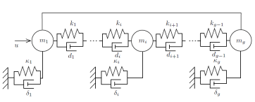
Here the th mass of the weight is connected to the mass by a spring and a damper with constants and , and also to the ground by a spring and a damper with the constants and , respectively. Furthermore, the first and the last mass points are connected by a rigid bar. The vibrations are driven by an external force , the control input, acting on the first mass point. The resulting system has a mass matrix , symmetric positive definite tridiagonal stiffness and damping matrices , , a constraint matrix , and an input matrix . Since and are symmetric positive definite, the problem can be formulated as a pHDAE of (Kronecker) index two by replacing the algebraic constraint by its first derivative yielding the pHDAE
| (8.28) |
with when adding an associated output equation .
The structure of the equations allows an easy construction of the condensed form required for the MOR methods. Performing a full rank decomposition of as with invertible and an orthogonal matrix , a congruence transformation yields the system
The last equation implies that . Differentiating this equation and inserting it into the second equation yields the hidden constraint for the Lagrange multiplier
which imposes a consistency condition for the initial value. The underlying pHODE of size together with the output equation are given by
| (8.29a) | ||||
| (8.29b) | ||||
If we permute the columns and rows such that the pHODE (8.29) is in the leading blocks, then we can mimic the MOR strategies from the previous subsections also for the pHDAE systems of (Kronecker) index two, by only reducing the pHODE (8.29). Note that the lower-right block matrix has no skew-symmetric contribution and hence the relevant submatrix for the FCRM is singular. We thus exclude FCRM in the following.
For our numerical example, we choose a similar setting as in [106] with parameters as listed in Table 1.
| parameter | ||||||||||
|---|---|---|---|---|---|---|---|---|---|---|
| value |
To compute a ROM with the different methods, we pick and reduce only the pHODE (8.29) while the algebraic part is not reduced, knowing that, in general, this is not optimal (cf. Remark 8.10). Whenever we report a reduced dimension , this means that one has to add the number of algebraic equations to the dimension of the ROM. A frequency sweep for the different ROMs with is presented in Figure 5 and relative -norms for different values of are reported in Figure 6.
For the ROMs with , cf. Figure 5, we observe that MM with shift and yields outstanding approximations (errors of order ) for high and low frequencies, respectively. ECRM and rational interpolation with interpolation points computed via IRKA as described in Section 8.4, in contrast, provides a uniformly good approximation quality of order , independently of the chosen frequency. As already discussed before, the structure-preserving variant of IRKA cannot satisfy all the necessary optimality conditions. To improve the situation, we also present the error for tangential interpolation via structure-preserving IRKA with a modified Hamiltonian, denoted as IRKA (mod. ) in the figures, as described in (8.27), which yields a significant improvement over the original formulation. This can also be seen in the relative -errors displayed in Figure 6, where for , the IRKA-reduced pHDAE with modified Hamiltonian yields an approximation that is at least one order of magnitude better.
9. Temporal discretization and linear system solvers
In this section, we discuss the time-discretization of dHDAE and pHDAE systems and the associated linear system solves. The numerical solution of initial and boundary value problems for general DAE systems of the form (2.1a) has been an important research topic, see the monographs [41, 102, 104, 138]. Following the approach discussed in [126, Cha. 6], we may assume that the DAE is represented at every time-step in one of the strangeness-free forms (2.16) or (2.18), and then it has been shown that many implicit one-step and multi-step methods can be applied and have the same convergence order as for ODE systems.
9.1. Time discretization for pHDAEs
Most of the classical time-discretization techniques do not respect a given dHDAE or pHDAE structure in such a way that the time-discretized system still satisfies a power-balance equation or dissipation inequality. To analyze for which approaches this is guaranteed is an active research area that is proceeding in different directions. A very promising approach is the discretization of pHDAE systems in such a way, that the time-discrete system satisfies a discrete version of the power-balance equation, see [56, 120, 121] for pHODE systems, and [162, 165] for pHDAE systems. Another class of methods, particularly for non-dissipative ODE methods, is based on energy preserving geometric integration, see e.g., [57, 103, 180]. The analysis and comparison of these techniques is a topic on its own, so we only briefly discuss the approach based on collocation methods for pHDAEs of the form (4.1) in [162].
Consider an autonomous pHDAE of the form (4.1) with a given input function , a consistent initial value , and suppose that we want to approximate the solution in a time interval by a polynomial of degree at most . For a collocation method, the polynomial is chosen such that satisfies the pHDAE (4.1) in the collocation points with for .
Let denote the -th Lagrange interpolation polynomial with respect to the nodes , i.e.
Then for collocation methods one requires that
for the values , and also
where the coefficients and , are the coefficients of the Butcher diagram of the associated Runge-Kutta method, see [103].
To preserve the pHDAE structure one uses the Dirac structure as described in (6.4) associated to the pHDAE (4.1) and defines the Dirac structure associated to the time-discretization
with and , where
In this way one obtains a system that is equivalent to the approach of applying the collocation method and then computing discrete inputs and outputs , for , and then introduces the associated collocation flows, efforts, input and output as
In this way the discrete values are in in all collocation points and the discretization preserves the structure. To see this, let us consider the evolution of the Hamiltonian along the collocation polynomial . For this, let . Then we have
and in the collocation points the power balance equation is satisfied, i.e.
for . Applying the quadrature rule associated to the collocation method to evaluate the integral, we get
where is the approximation order of the quadrature rule. With the same argument we get
| (9.2a) | ||||
| (9.2b) | ||||
and hence
If , then (9.2a) and (9.2b) are even exact, and, if for , as is the case for many collocation methods, we have that , thus the discrete system satisfies the same qualitative behaviour as the continuous problem.
If the Hamiltonian is quadratic, i.e.
for some , and , then we have that and are polynomials of degree and degree , respectively. Using the well-known fact, see e.g. [104], that the maximum degree of exactness for quadrature rules with nodes is , and that it is attained only with Gauß-Legendre collocation methods, it follows that for these methods the integration of is exact, i.e.
Since furthermore, for these methods we have , it follows that the dissipation term is always non-positive, and we obtain the discrete version of the dissipation inequality
hence for quadratic Hamiltonians the pHDAE structure is fully preserved.
Example 9.1.
Consider the numerical solution of the strangeness-free dHDAE system, given by the power network presented in Section 5.2. We use the artificial constants , , , , , and , see [162]. For the time integration we choose and and use the implicit midpoint rule, i.e., the Gauß-Legendre collocation method with stages and order . The numerical result for the consistent initial value
is presented in Figure 7. One observes that after an initial phase the state converges to zero and the Hamiltonian decreases monotonically.
9.2. Linear System Solvers
In every step of an implicit time-discretization method for a finite dimensional pHDAE system, it is necessary to solve linear algebraic systems of the form
| (9.3) |
where is the time-stepsize. The matrix can be split in its symmetric and skew-symmetric part , where and . An analogous linear system structure occurs in discretized linear time-varying and nonlinear pHDAE systems, in the construction of reduced models [71], and by multiplying some equations with in optimization methods,see also [92, 153].
The fact that the symmetric part is positive semi-definite can be exploited in direct or iterative solution methods. In the small and medium scale case we can make use of the following staircase form, see [2], which we present here in the real case.
Lemma 9.2.
Consider , where and . Then there exist a real orthogonal matrix , and integers and , such that
| (9.4) |
where is positive definite, for , and with being nonsingular for .
Proof.
We present the proof for completeness, see also [92]. The result is trivial when is nonsingular (and thus positive definite), since in this case it holds with , , , and .
Let be singular. We consider a full rank decomposition of with a real orthogonal such that
where we assume that , with , is void or positive definite. Applying the same orthogonal congruence transformation to gives the matrix
| (9.5) |
where , and , since is skew-symmetric. If is void or , then the proof is complete. Otherwise, let
be a singular value decomposition, where is nonsingular (and diagonal), and , are real orthogonal. We define and form
where is void or symmetric positive definite, and
with . If or is void then the proof is again complete. Otherwise we continue inductively and after finitely many steps we obtain a decomposition of the required form. ∎
When the staircase form (9.4) has been computed, then the transformed linear system can be solved using block Gaussian elimination.
Lemma 9.3.
Consider the matrix in (9.4). Then there exist invertible lower and upper block bi-diagonal matrices , respectively, such that
with Schur complements that have positive definite symmetric parts.
Proof.
A constructive proof via a sequence of block Gaussian elimination steps is given in [92]. It relies on the fact that in every step (except the last one) the Schur complement has a symmetric part which is positive definite. ∎
The properties of the linear system resulting from the dHDAE structure also have an immediate advantage in the context of iterative methods. If the symmetric part is positive definite then in [229] it is suggested to solve, instead of , the equivalent system
| (9.6) |
This transformation is a left preconditioning of the original system with its positive definite symmetric part, which defines the -inner product
This implies that one can construct optimal Krylov subspace methods based on three-term recurrences for the system (9.6), see [187, 229]. If the symmetric part is semi-definite but singular, then one has to identify the nullspace, which is actually easy in many applications. The advantages of this approach and the fact that one obtains a rigorous convergence analysis and optimality conditions is discussed in detail in [92] and illustrated with several numerical examples including those discussed in Section 5.
Example 9.4.
The finite element model of the disk brake discussed in Section 5.7 leads to a second order DAE of the form
with the coefficient vector of displacements of the structure, with frequency dependent mass matrix , damping matrix , and stiffness matrix , see [89] evaluated for . For , after a first-order reformulation and discretization with the implicit mid-point rule one obtains a linear system with and a positive definite symmetric part.
As shown in Table 2, a preconditioned GMRES methods (preconditioned with the inverse of the symmetric part), even though using fewer iterations, takes a significantly longer time than the method in [229], due to the full recurrences in the algorithm compared to three-term recurrences in Widlund’s method. This effect becomes even more pronounced for smaller stepsizes.
| method | time [s] | # of iter. | time [s] | # of iter |
|---|---|---|---|---|
| Widlund | 3.54 | 85 | 0.72 | 16 |
| GMRES | 31.10 | 65 | 10.51 | 13 |
10. Control methods for pHDAE systems
One of the main advantages to introduce pH descriptor systems is its direct base in control theory. In this section we therefore discuss classical control applications for pHDAE systems.
Consider a linear pHDAE system as in Definition 4.8 and a linear output feedback . Then, we can write the system in behavior form by introducing and new block matrices
as well as
| (10.1) |
which gives the closed-loop descriptor system
| (10.2) |
This is a dHDAE if and only if pointwise.
Analogously, for the general nonlinear pHDAE structure in Definition 4.1, we introduce
the Hamiltonian and matrix functions , and and as defined in (10.1). This gives the system in behavior form
| (10.3) |
satisfying and pointwise, which is a pHDAE if and only if pointwise.
In this way, using a parameterization via the output feedback matrix (function) , we can introduce control methods via the dHDAE systems (10.2) or (10.3), respectively.
10.1. Robust stabilization/passivation
We have seen in Section 7.6 that for dHDAE systems, stability and passivity can be easily characterized, while for asymptotic stability or strict passivity, in general, we have only sufficient conditions.
Considering a linear pHDAE system of the form (4.5) with that has no feedthrough term (cf. Section 4.4), and using a linear output feedback we obtain the closed-loop system
If is chosen to have a negative semi-definite symmetric part , then the new dissipation coefficient becomes and the skew-symmetric part becomes . If is positive definite then the system is asymptotically stable. The same approach can also be applied in the general nonlinear case, if an output feedback leads to a positive definite in (4.1). We only have this sufficient condition to guarantee asymptotic stability, see Corollary 7.29. At current, the problem to find a necessary and sufficient condition that guarantees that a pHDAE system can be made asymptotically stable by output feedback is under investigation.
The situation is much better understood in the case of LTI pHDAE systems, where we have a characterization via the hypocoercivity index being finite in Corollary 7.22. Then in view of Theorem 7.20 (ii), we have different options to obtain asymptotic stability.
Again, if we can achieve , then we have asymptotic stability. But we can also use the skew part to change the eigenvectors of the pair in such a way that no eigenvector is in the kernel of , or we can use a combination of both. It is clear from the classical theory of unstructured DAE systems, see Section 3.3, that if the system is strongly stabilizable and strongly detectable, then such an output feedback exists and can be computed by ignoring the structure and solving an optimal control problem.
In constructing an output feedback via optimal control methods, we have the freedom to choose the cost functional (3.20) and, furthermore, we also have some freedom in choosing the pHDAE representation, which is not unique (see, for instance, the discussion at the end of Section 8.4). This flexibility can be used to make the resulting closed-loop system maximally robust against perturbations, which for general LTI control systems recently has been an important research topic, see e.g., [164] and the references therein. For pHODE systems, this topic has recently been of great importance by introducing measures like the distance to instability for the robustness of pHODE representations, see [6], as well as their optimization [87, 88]. For pHDAE systems, this is currently an active research topic.
The analogous question arises in the context of passivity. We have that a regular strangeness-free pHDAE system is passive, but in general not necessarily strictly passive, since in (4.8) is only assumed positive semi-definite. To obtain strict passivity, it is necessary to consider the system in the formulation with feedthrough term and similarly we can analyze how to obtain robust representations as is done for pHODE systems in [20, 24, 161]. For pHDAE systems, this is again an active research topic.
10.2. Optimal control
Due to the many interesting properties of pHDAE systems, one may investigate whether some extra advantages can be obtained also in the context of optimal control problems. Clearly one can just use the general results in Section 3.5 and obtain the same optimality conditions. However, it has been observed in two recent papers, see [173, 76], that some surprising results arise for optimal control problems with LTI pHODE and pHDAE, when as very special cost functional the supplied energy is minimized, i.e.
| (10.4) |
subject to the constraint
| (10.5) |
and the output equation is . Note that in the cost functional (3.32) we then have , , and . Since we are in the LTI case, we can insert the data into the optimality system (3.34) and obtain the following result.
Corollary 10.1.
Consider the optimal control problem to minimize (10.4) subject to the constraint (10.5). Assume that the pair is regular and of (Kronecker) index at most one (as a free system with ) and that is in . If is a solution to this optimal control problem, then there exists a Lagrange multiplier , such that satisfy the boundary value problem
| (10.6) |
with boundary conditions
Use a full rank decomposition with and transform the other coefficients accordingly as
After some permutations we can express (10.6) in the form
| (10.7) |
with boundary conditions and , and consistency condition . Here we have used the condition that is in , which implies that , .
For the structured matrix pencil associated with (10.7) there exists a condensed form under real orthogonal congruence transformations, which has been introduced in [50], and from which the spectral properties, the (Kronecker) index and the regularity can be read off. If this pencil is regular, then we directly obtain that the system has (Kronecker) index one if and only if
is invertible, see Section 2.3. To simplify the algebraic equations, we can perform a congruence transformation with the orthogonal matrix
i.e., we multiply the system with from the left and set
Then we get that
Clearly, for this to be invertible, we need that has full column rank, which implies that is fixed as a linear combination of and . Considering the application examples in Section 5, where we typically have , we cannot expect the DAE associated with the optimality system to be of (Kronecker) index one. Thus we are in the case of a singular control problem, see e.g., [44].
The case that is not invertible has been analyzed in [200] for the pHODE case and in [76] for the pHDAE case, where is regular and of (Kronecker) index at most one. In these papers, it is assumed that the image of the matrix does not intersect with the kernel of and that even though this is a singular control problem, the optimal solution is still a feedback control that can be obtained via the solution of a Riccati equation. We refer to [15] for the analysis of such problems. The extension of this analysis to the LTV pHDAE case and the case that this assumption is not valid is currently under investigation.
11. Summary and open problems
This survey paper discusses the model class of port-Hamiltonian descriptor systems (differential-algebraic systems) for numerical simulation and control. We have demonstrated that this model class has many nice properties:
-
•
It allows for automated modeling in a modularized and network-based fashion.
-
•
It allows the coupling of mathematical models across different scales and physical domains.
-
•
It incorporates the properties of the real (open or closed) physical system.
-
•
It has nice algebraic, geometric, and analytical properties and allows analysis concerning existence, uniqueness, robustness, stability, and passivity.
-
•
It is invariant under local variable (coordinate) transformations which leads to local canonical and condensed forms.
-
•
Furthermore, it allows for structure-preserving (space-time) discretization and model reduction methods as well as fast solvers for the resulting linear and nonlinear systems of equations.
Despite the many promising results already available for pHDAEs, there are still many open problems that are either under investigation or pose challenging problems to be tackled in the future. In the following, we present an incomplete list to stimulate further research.
Many of the control theoretical concepts presented within this paper rely on instantaneous feedback. While this is a convenient theoretical approach, it is not always possible to realize in applications, where the states or outputs first have to be measured, the control action computed, and then fed back to the system, thus resulting in a necessary intrinsic time delay; see also Remark 3.5. Although some first results for pHODEs with delays are available in the literature, see for instance [202], a general model class for time-delayed pHDAEs is not yet available and the results presented in this paper have to be extended to the time-delay case.
In terms of MOR, the impact of the Hamiltonian on the approximation quality, see [38, 40], needs to be further investigated, in particular with an emphasis on nonlinear MOR methods. Structure-preserving balancing methods are still under investigation; see [39] for some first results for LTI systems. Another open problem in structure-preserving MOR is the construction of optimal projection spaces, in the sense that they minimize the Kolmogorov -widths, respectively the Hankel singular values, cf. [222]. First gradient-based optimization procedures are discussed for pHODEs in [166, 199, 208]. If the -widths do not decay rapidly, then one cannot expect accurate ROMs with a small dimension and current efforts in the reduction of transport-dominated phenomena, see for instance [36] and the references therein, need to be adapted to the pH framework.
A closely related topic to MOR is identifying a pHDAE realization from measurements. In view of large data sets, modern artificial intelligence approaches, and automatized machine learning methods used within the digital twin paradigm, this is an important topic requiring further research, with only a few available results for LTI systems, see Remark 8.15.
It is an open problem to derive necessary and sufficient conditions under which output feedback can make a general nonlinear pHDAE system asymptotically stable. A natural research question in this context would be to extend the concept of hypocoercivity to the LTV and nonlinear case.
The characterization of distance measures for general dHDAE systems, like the distance from an asymptotically stable dHDAE system to a system which is only stable or the distance of a strictly passive pHDAE system to the nearest system that is only passive, is an important research topic because it is a requirement for the design of real-world systems, as e.g., in Section 5.7. Even if such a characterization is available, then one needs computational methods to compute these distances. In the large-scale setting, this is a challenging issue that can only be achieved with a clever combination with model reduction techniques; see [6] for a first attempt.
Another important research problem is the exact characterization of the relationship between passivity, positive realness, and the port-Hamiltonian structure for pHDAEs, see [24, 25] for the pHODE case, as well as the characterization via Kalman-Yakobovich-Popov inequalities as it has been done for general LTI DAE systems in [190, 193].
A research field that has so far not received much attention are discrete-time pH descriptor systems. The primary research in this direction arises from discretizations of pHDAE systems, see [120, 162] for the most recent approaches. Since discrete-time systems not only arise from discretization but also from sampling or realization, it is an open question how to properly define discrete-time pH systems in a general way. This also concerns the stability and passivity analysis. An approach to modifying the concept of hypocoercivity for use in discrete-time systems is currently under investigation.
Since, in many cases, mathematical models are obtained from data via measurements, and the resulting parameters, as well as model coefficients (including the inputs and outputs), are only available with some uncertainty or randomness, it is an open question to include such uncertainties adequately into the pHDAE framework and also to study robust control methods that deal with such uncertainties, see [38, 39] for the modification of classical balanced truncation methods and [117] for the modification of robust control methods in the pHODE case. Another research area is the perturbation theory for the problems and the error analysis of the relevant numerical methods.
As we have seen, also the area of optimal control for pHDAE systems requires a lot of further research. This concerns, in particular, the optimal use of the structure for nonlinear systems, the choice of an appropriate cost functional, and also structure-preserving numerical methods in particular for large-scale problems.
Finally, we would like to discuss a topic that has only briefly been touched on in this survey: the extension of pH modeling to partial differential equations that has been pursued in many different directions in recent years. One can take the approach to replace the coefficient matrices with linear differential operators, one can follow a differential geometric approach via the extension of Lagrange or Dirac structures, or one can formulate all classical partial differential equations from physics in the areas of elasticity, electromagnetism, fluid dynamics, structural mechanics, geomechanics, poroelasticity, gas or water transport, to name a few directions, in a structure that resembles the pHDAE structure via the given symmetries or differential forms. These efforts have been the topic of many recent research papers on modeling, numerical methods, optimization, and control. Discussing these developments would be a considerable survey on its own, mainly since the field is growing immensely fast. An essential question that is widely open is to incorporate the boundary appropriately into the structure, to obtain well-posed partial differential equations and so that they, on the one hand, can be treated as controls and, on the other hand, also be used for the interconnection of subsystems. Another important topic that is actively pursued is appropriate time space-time discretization methods like finite element or finite volume approaches that preserve the structure.
Instead of discussing this further, we present the following incomplete list of references that describes many different research directions pursued: [7, 8, 14, 16, 21, 55, 68, 69, 70, 71, 75, 115, 83, 84, 91, 119, 121, 135, 141, 148, 149, 150, 151, 154, 165, 168, 167, 170, 171, 184, 226, 203, 210, 228, 234, 235].
Acknowledgments
The work of V. Mehrmann has been supported by the Deutsche Forschungsgemeinschaft (DFG, German Research Foundation) CRC 910 Control of self-organizing nonlinear systems: Theoretical methods and concepts of application: Project No. 163436311, CRC TRR 154 Mathematical modeling, simulation and optimization at the example of gas networks: Project No. 239904186, priority programs SPP 1984 Hybrid and multimodal energy systems: System theoretical methods for the transformation and operation of complex networks: Project No. 361092219, and SPP 1897, Calm, Smooth and Smart - Novel Approaches for Influencing Vibrations by Means of Deliberately Introduced Dissipation: Project No. 273845692, DFG Excellence Cluster 2046 Math+: Project No. 390685689, as well as the BMBF (German Ministry of Education and Research) via the Project EiFer.
B. Unger acknowledges funding from the DFG under Germany’s Excellence Strategy – EXC 2075 – 390740016 and is thankful for support by the Stuttgart Center for Simulation Science (SimTech).
References
- [1] F. Achleitner, A. Arnold, and E.A. Carlen. The hypocoercivity index for the short and large time behavior of ODEs. ArXiv e-print 2109.10784, 2021.
- [2] F. Achleitner, A. Arnold, and V. Mehrmann. Hypocoercivity and controllability in linear semi-dissipative ODEs and DAEs. ZAMM Z. Angew. Math. Mech., In Press, 2021.
- [3] L. Ya. Adrianova. Introduction to linear systems of differential equations. Trans. Math. Monographs, Vol. 146, AMS, Providence, RI, 1995.
- [4] B. M. Afkham and J. S. Hesthaven. Structure preserving model reduction of parametric Hamiltonian systems. SIAM J. Sci. Comput., 39(6):A2616–A2644, 2017.
- [5] B. M. Afkham and J. S. Hesthaven. Structure-preserving model-reduction of dissipative Hamiltonian systems. J. Sci. Comput., 81:3–21, 2019.
- [6] N. Aliyev, V. Mehrmann, and E. Mengi. Computation of stability radii for large-scale dissipative Hamiltonian systems. Adv. Comput. Math., 46(6):1–28, 2020.
- [7] R. Altmann, V. Mehrmann, and B. Unger. Port-Hamiltonian formulations of poroelastic network models. Math. Comput. Model. Dyn. Sys., 27(1):429–452, 2021.
- [8] R. Altmann and P. Schulze. A port-Hamiltonian formulation of the Navier-Stokes equations for reactive flows. Systems Control Lett., 100:51–55, 2017.
- [9] A. C. Antoulas. Approximation of large-scale dynamical systems. Advances in Design and Control. Society for Industrial and Applied Mathematics, Philadelphia, PA, USA, 2005.
- [10] A. C. Antoulas. A new result on passivity preserving model reduction. Systems Control Lett., 54:361–374, 2005.
- [11] A. C. Antoulas. On the construction of passive models from frequency response data. at - Automatisierungstechnik, 56(8):447–452, 2008.
- [12] A. C. Antoulas, C. A. Beattie, and S. Gugercin. Interpolatory Methods for Model Reduction. Computational Science & Engineering. Society for Industrial and Applied Mathematics, Philadelphia, PA, USA, 2020.
- [13] A. C. Antoulas, S. Lefteriu, and A. C. Ionita. Chapter 8: A tutorial introduction to the Loewner framework for model reduction. In P. Benner, A. Cohen, M. Ohlberger, and K. Willcox, editors, Model Reduction and Approximation, pages 335–376. Society for Industrial and Applied Mathematics, Philadelphia, PA, USA, 2017.
- [14] S. Aoues, F. L. Cardoso-Ribeiro, D. Matignon, and D. Alazard. Modeling and control of a rotating flexible spacecraft: A port-Hamiltonian approach. IEEE Trans. Control Sys. Tech., 27(1):355–362, 2017.
- [15] M. S. Aronna. Second order necessary and sufficient optimality conditions for singular solutions of partially-affine control problems. Discrete Contin. Dyn. Syst., 11:1179–1199, 2018.
- [16] A. Baaiu, F. Couenne, D. Eberard, C. Jallut, Y. Legorrec, L. Lefèvre, and B. Maschke. Port-based modelling of mass transport phenomena. Math. Comput. Model. Dyn. Sys., 15(3):233–254, 2009.
- [17] A. Backes. Optimale Steuerung der linearen DAE im Fall Index 2. Dissertation, Humboldt-Universität zu Berlin, 2006.
- [18] M. Bai, D. Elsworth, and J.-C. Roegiers. Multiporosity/multipermeability approach to the simulation of naturally fractured reservoirs. Water Resourc. Res., 29(6):1621–1633, 1993.
- [19] Z. Bai. Krylov subspace techniques for reduced-order modeling of large-scale dynamical systems. Appl. Numer. Math., 43(1–2):9–44, 2002.
- [20] D. Bankmann, V. Mehrmann, Y. Nesterov, and P. Van Dooren. Computation of the analytic center of the solution set of the linear matrix inequality arising in continuous- and discrete-time passivity analysis. Vietnam J. Math., 48:633–660, 2020.
- [21] H. Bansal, P. Schulze, M. H. Abbasi, H. Zwart, L. Iapichino, W. H. A. Schilders, and N. Wouw. Port-Hamiltonian formulation of two-phase flow models. Systems Control Lett., 149:104881, 2021.
- [22] M. Barrault, Y. Maday, N. C. Nguyen, and A. T. Patera. An ’empirical interpolation’ method: application to efficient reduced-basis discretization of partial differential equations. C. R. Math. Acad. Sci. Paris, 339(9):667–672, 2004.
- [23] C. Beattie and S. Gugercin. Structure-preserving model reduction for nonlinear port-Hamiltonian systems. In 50th IEEE Conference on Decision and Control and European Control Conference (CDC-ECC), 2011, pages 6564–6569, 2011.
- [24] C. Beattie, V. Mehrmann, and P. Van Dooren. Robust port-Hamiltonian representations of passive systems. Automatica J. IFAC, 100:182–186, 2019.
- [25] C. Beattie, V. Mehrmann, and H. Xu. Port-Hamiltonian realizations of linear time invariant systems. Preprint 23-2015, Institut für Mathematik, Technische Universität Berlin, 2015. ArXiv e-print.
- [26] C. Beattie, V. Mehrmann, H. Xu, and H. Zwart. Port-Hamiltonian descriptor systems. Math. Control Signals Systems, 30(17):1–27, 2018.
- [27] C. A. Beattie, S. Gugercin, and V. Mehrmann. Structure-preserving interpolatory model reduction for port-Hamiltonian differential-algebraic systems. ArXiv e-print 1910.05674, 2019. To appear in Festschrift to honor the 70th birthday of A. Antoulas.
- [28] A. Beckesch. Pfadverfolgung für Finite-Elemente-Modelle parametrischer mechanischer Systeme. Master thesis, Technische Universität Berlin, 2018.
- [29] P. Benner, A. Cohen, M. Ohlberger, and K. Willcox. Model Reduction and Approximation. Computational Science & Engineering. Society for Industrial and Applied Mathematics, Philadelphia, PA, 2017.
- [30] P. Benner, P. Goyal, and P. Van Dooren. Identification of port-Hamiltonian systems from frequency response data. Systems Control Lett., 143:104741, 2020.
- [31] P. Benner and V. I. Sokolov. Partial realization of descriptor systems. Systems Control Lett., 55(11):929–938, 2006.
- [32] T. Berger. Bohl exponent for time-varying linear differential-algebraic equations. Internat. J. Control, 85(10):1433–1451, 2012.
- [33] T. Berger and T. Reis. Controllability of linear differential-algebraic equations – a survey. In A. Ilchmann and T. Reis, editors, Surveys in Differential-Algebraic Equations I, Differential-Algebraic Equations Forum, pages 1–61. Springer-Verlag, Berlin, Heidelberg, 2013.
- [34] D. Bienstock. Electrical transmission system cascades and vulnerability: an operations research viewpoint. MOS-SIAM Series on Optimization. Society for Industrial and Applied Mathematics, Philadelphia, PA, 2015.
- [35] M. A. Biot. General theory of three-dimensional consolidation. J. Appl. Phys, 12(2):155–164, 1941.
- [36] F. Black, P. Schulze, and B. Unger. Projection-based model reduction with dynamically transformed modes. ESAIM: Math. Model. Numer. Anal., 54(6):2011–2043, 2020.
- [37] P. Borja, J. M. A. Scherpen, and K. Fujimoto. Extended balancing of continuous LTI systems: a structure-preserving approach. IEEE Trans. Automat. Control, 2021.
- [38] T. Breiten, R. Morandin, and P. Schulze. Error bounds for port-Hamiltonian model and controller reduction based on system balancing. Comput. Math. Appl., 2021. In press.
- [39] T. Breiten and P. Schulze. Structure-preserving linear quadratic gaussian balanced truncation for port-Hamiltonian descriptor systems. ArXiv e-print 2111.05065, 2021.
- [40] T. Breiten and B. Unger. Passivity preserving model reduction via spectral factorization. ArXiv e-print 2103.13194, 2021.
- [41] K. E. Brenan, S. L. Campbell, and L. R. Petzold. Numerical solution of initial-value problems in differential-algebraic equations. Society for Industrial and Applied Mathematics, Philadelphia, PA, 1996.
- [42] J. Brouwer, I. Gasser, and M. Herty. Gas pipeline models revisited: Model hierarchies, non-isothermal models and simulations of networks. Multiscale Model. Simul., 9:601–623, 2011.
- [43] T. Brown, D. Schlachtberger, A. Kies, S. Schramm, and M. Greiner. Synergies of sector coupling and transmission reinforcement in a cost-optimised, highly renewable european energy system. Energy, 160:720–739, 2018.
- [44] A. E. Bryson and Y.-C. Ho. Applied optimal control: optimization, estimation, and control. Routledge, Boca Raton, 2018.
- [45] P. Buchfink, S. Glas, and B. Haasdonk. Symplectic model reduction of Hamiltonian systems on nonlinear manifolds. ArXiv e-print 2112.10815, 2021.
- [46] A. Bunse-Gerstner, R. Byers, V. Mehrmann, and N. K. Nichols. Numerical computation of an analytic singular value decomposition of a matrix valued function. Numer. Math., 60(1):1–39, 1991.
- [47] A. Bunse-Gerstner, R. Byers, V. Mehrmann, and N. K. Nichols. Feedback design for regularizing descriptor systems. Linear Algebra Appl., 299(1–3):119–151, 1999.
- [48] R. Byers, T. Geerts, and V. Mehrmann. Descriptor systems without controllability at infinity. SIAM J. Cont., 35:462–479, 1997.
- [49] R. Byers, P. Kunkel, and V. Mehrmann. Regularization of linear descriptor systems with variable coefficients. SIAM J. Control Optim., 35(1):117–133, 1997.
- [50] R. Byers, V. Mehrmann, and H. Xu. A structured staircase algorithm for skew-symmetric/symmetric pencils. Electron. Trans. Numer. Anal., 26:1–13, 2007.
- [51] C. I. Byrnes, A. Isidori, and J. C. Willems. Passivity, feedback equivalence, and the global stabilization of minimum phase nonlinear systems. IEEE Trans. Automat. Control, 36:1228–1240, 1991.
- [52] S. L. Campbell. A general form for solvable linear time varying singular systems of differential equations. SIAM J. Math. Anal., 18:1101–1115, 1987.
- [53] S. L. Campbell and C. W. Gear. The index of general nonlinear DAEs. Numer. Math., 72(2):173–196, 1995.
- [54] S. L. Campbell, P. Kunkel, and V. Mehrmann. Regularization of linear and nonlinear descriptor systems. In L. T. Biegler, S. L. Campbell, and V. Mehrmann, editors, Control and Optimization with Differential-Algebraic Constraints, number 23 in Advances in Design and Control, pages 17–36. Society for Industrial and Applied Mathematics, 2012.
- [55] F. L. Cardoso-Ribeiro, D. Matignon, and V. Pommier-Budinger. A port-Hamiltonian model of liquid sloshing in moving containers and application to a fluid-structure system. J. Fluids Structures, 69:402–427, 2017.
- [56] E. Celledoni and E. H. Høiseth. Energy-preserving and passivity-consistent numerical discretization of port-Hamiltonian systems. ArXiv e-print 1706.08621, 2017.
- [57] E. Celledoni, R. I. McLachlan, D. I. McLaren, B. Owren, G. R. W. Quispel, and W. M. Wright. Energy-preserving Runge-Kutta methods. ESAIM: Math. Model. Numer. Anal., 43(4):645–649, 2009.
- [58] S. Chaturantabut, C. A. Beattie, and S. Gugercin. Structure-preserving model reduction for nonlinear port-Hamiltonian systems. SIAM J. Sci. Comput., 38(5):B837–B865, 2016.
- [59] S. Chaturantabut and D. Sorensen. Nonlinear model reduction via discrete empirical interpolation. SIAM J. Sci. Comput., 32(5):2737–2764, 2010.
- [60] K. Cherifi, V. Mehrmann, and K. Hariche. Numerical methods to compute a minimal realization of a port-Hamiltonian system. ArXiv e-print 1903.07042, 2019.
- [61] A. J. Conejo, S. Chen, and G. E. Constante. Operations and long-term expansion planning of natural-gas and power systems: a market perspective. Proc. IEEE, 108(9):1541–1557, 2020.
- [62] L. Dai. Singular Control Systems, volume 118 of Lecture Notes in Control and Inform. Sci. Springer-Verlag, Berlin, Heidelberg, 1989.
- [63] U. B. Desai and D. Pal. A transformation approach to stochastic model reduction. IEEE Trans. Automat. Control, 29(12):1097–1100, 1984.
- [64] L. Dieci and T. Eirola. On smooth decompositions of matrices. SIAM J. Matrix Anal. Appl., 20:800–819, 1999.
- [65] L. Dieci, R. D. Russell, and E. S. Van Vleck. On the computation of Lyapunov exponents for continuous dynamical systems. SIAM J. Numer. Anal., 34:402–423, 1997.
- [66] L. Dieci and E. S. Van Vleck. Lyapunov and other spectra: a survey. In Collected lectures on the preservation of stability under discretization (Fort Collins, CO, 2001), pages 197–218. Society for Industrial and Applied Mathematics, Philadelphia, PA, 2002.
- [67] N. H. Du, V. H. Linh, and V. Mehrmann. Robust stability of differential-algebraic equations. In Surveys in Differential-Algebraic Equations. I, pages 63–95. Springer-Verlag, Berlin, 2013.
- [68] V. Duindam, A. Macchelli, S. Stramigioli, and H. Bruyninckx. Modeling and control of complex physical systems: the port-Hamiltonian approach. Springer-Verlag, Berlin, Heidelberg, 2009.
- [69] H. Egger. Structure preserving approximation of dissipative evolution problems. Numer. Math., 143(1):85–106, 2019.
- [70] H. Egger and T. Kugler. Damped wave systems on networks: Exponential stability and uniform approximations. Numer. Math., 138(4):839–867, 2018.
- [71] H. Egger, T. Kugler, B. Liljegren-Sailer, N. Marheineke, and V. Mehrmann. On structure preserving model reduction for damped wave propagation in transport networks. SIAM J. Sci. Comput., 40:A331–A365, 2018.
- [72] H. Egger and M. Sabouri. On the structure preserving high-order approximation of quasistatic poroelasticity. Math. and Comp. in Simulation, 189:237–252, 2021.
- [73] E. Eich-Soellner and C. Führer. Numerical Methods in Multibody Dynamics. Vieweg+Teubner Verlag, Wiesbaden, 1998.
- [74] E. Emmrich and V. Mehrmann. Operator differential-algebraic equations arising in fluid dynamics. Comput. Methods Appl. Math, 13(4):443–470, 2013.
- [75] H. Ennsbrunner and K. Schlacher. On the geometrical representation and interconnection of infinite dimensional port controlled Hamiltonian systems. In Proceedings of the 44th IEEE Conference on Decision and Control, pages 5263–5268. IEEE, 2005.
- [76] T. Faulwasser, B. Maschke, F. Philipp, M. Schaller, and K. Worthmann. Optimal control of port-Hamiltonian descriptor systems with minimal energy supply. ArXiv e-preprint 2106.06571, 2021.
- [77] R. W. Freund. Krylov-subspace methods for reduced-order modeling in circuit simulation. J. Comput. Appl. Math., 123:395–421, 2000.
- [78] R. W. Freund. Padé-type model reduction of second-order and higher-order linear dynamical systems. In P. Benner, D. C. Sorensen, and V. Mehrmann, editors, Dimension Reduction of Large-Scale Systems, pages 191–223. Springer-Verlag, Berlin, Heidelberg, 2005.
- [79] R. W. Freund. The SPRIM algorithm for structure-preserving order reduction of general RLC circuits. In P. Benner, M. Hinze, and E. J. W. ter Maten, editors, Model reduction for circuit simulation, pages 25–52. Springer-Verlag, Dordrecht, 2011.
- [80] K. O. Friedrichs and P. D. Lax. Systems of conservation equations with a convex extension. Proc. Nat. Acad. Sci. U.S.A., 68(8):1686–1688, 1971.
- [81] K. Fujimoto and H. Kajiura. Balanced realization and model reduction of port-Hamiltonian systems. In 2007 American Control Conference, pages 930–934, 2007.
- [82] F.R. Gantmacher. The Theory of Matrices, volume 2. Chelsea, New York, 1959.
- [83] F. Gay-Balmaz and H. Yoshimura. Dirac structures in nonequilibrium thermodynamics. J. Math. Phys., 59(1):012701, 2018.
- [84] F. Gay-Balmaz and H. Yoshimura. From Lagranian mechanics to nonequilibrium thermodynamics: a variational perspective. Entropy, 21(1):8, 2019.
- [85] H. Gernandt and F. E. Haller. On the stability of port-Hamiltonian descriptor systems. IFAC-PapersOnLine, 54(19):137–142, 2021.
- [86] H. Gernandt, F. E. Haller, and E. Reis. A linear relation approach to port-Hamiltonian differential-algebraic equations. SIAM J. Matrix Anal. Appl., 42(2):1011–1044, 2021.
- [87] N. Gillis, V. Mehrmann, and P. Sharma. Computing the nearest stable matrix pairs. Numer. Lin. Alg. Appl., 25(5):e2153, 2018.
- [88] N. Gillis and P. Sharma. On computing the distance to stability for matrices using linear dissipative Hamiltonian systems. Automatica J. IFAC, 85:113–121, 2017.
- [89] N. Gräbner, V. Mehrmann, S. Quraishi, C. Schröder, and U. von Wagner. Numerical methods for parametric model reduction in the simulation of disc brake squeal. ZAMM Z. Angew. Math. Mech., 96:1388–1405, 2016.
- [90] E. J. Grimme. Krylov projection methods for model reduction. PhD thesis, University of Illinois, Urbana-Champaign, 1997.
- [91] M. Grmela and H. C. Öttinger. Dynamics and thermodynamics of complex fluids. I. Development of a general formalism. Phys. Rev. E, 56(6):6620–6632, 1997.
- [92] C. Güdücü, J. Liesen, V. Mehrmann, and D. Szyld. On non-Hermitian positive (semi)definite linear algebraic systems arising from dissipative Hamiltonian DAEs. ArXiv e-print 2111.05616, 2021.
- [93] S. Gugercin and A. C. Antoulas. A survey of model reduction by balanced truncation and some new results. Internat. J. Control, 77:748–766, 2004.
- [94] S. Gugercin, A. C. Antoulas, and C. A. Beattie. Model Reduction for Large-Scale Linear Dynamical Systems. SIAM J. Matrix Anal. Appl., 30(2):609–638, 2008.
- [95] S. Gugercin, R. V. Polyuga, C. Beattie, and A. van der Schaft. Interpolation-based model reduction for port-Hamiltonian systems. In Proceedings 48th IEEE Conference on Decision and Control, pages 5362–5369, 2009.
- [96] S. Gugercin, Rostyslav V. Polyuga, C. Beattie, and A. van der Schaft. Structure-preserving tangential interpolation for model reduction of port-Hamiltonian systems. Automatica J. IFAC, 48(9):1963–1974, 2012.
- [97] S. Gugercin, T. Stykel, and S. Wyatt. Model reduction of descriptor systems by interpolatory projection methods. SIAM J. Sci. Comput., 35(5):B1010–B1033, 2013.
- [98] N. Guglielmi and V. Mehrmann. Computation of the nearest structured matrix triplet with common null space. ArXiv e-print 2109.05737, 2021.
- [99] C. Guiver and M. R. Opmeer. Error bounds in the gap metric for dissipative balanced approximations. Linear Algebra Appl., 439:3659–3698, 2013.
- [100] M. Günther, A. Bartel, B. Jacob, and T. Reis. Dynamic iteration schemes and port-Hamiltonian formulation in coupled differential-algebraic equation circuit simulation. Int J. Circ. Theor. Appl., 49(2):430–452, 2021.
- [101] B. Haasdonk. Chapter 2: Reduced basis methods for parametrized PDEs – a tutorial introduction for stationary and instationary problems. In P. Benner, A. Cohen, M. Ohlberger, and K. Willcox, editors, Model Reduction and Approximation, pages 65–136. Society for Industrial and Applied Mathematics, Philadelphia, PA, USA, 2017.
- [102] E. Hairer, C. Lubich, and M. Roche. The Numerical Solution of Differential-Algebraic Systems by Runge-Kutta Methods. Springer-Verlag, Berlin, Heidelberg, 1989.
- [103] E. Hairer, C. Lubich, and G. Wanner. Geometric Numerical Integration. Structure-Preserving Algorithms for Ordinary Differential Equations. Springer-Verlag, Berlin, Heidelberg, 2002.
- [104] E. Hairer and G. Wanner. Solving Ordinary Differential Equations II: Stiff and Differential-Algebraic Problems. Springer-Verlag, Berlin, Germany, 2nd edition, 1996.
- [105] P. Hamann and V. Mehrmann. Numerical solution of hybrid systems of differential-algebraic equations. Comput. Meth. Appl. Mech. Eng., 197(6–8):693–705, 2008.
- [106] S.-A. Hauschild, N. Marheineke, and V. Mehrmann. Model reduction techniques for linear constant coefficient port-Hamiltonian differential-algebraic systems. Control & Cybernetics, 48:125–152, 2019.
- [107] M. Heinkenschloss, D. C. Sorensen, and K. Sun. Balanced truncation model reduction for a class of descriptor systems with application to the Oseen equations. SIAM J. Sci. Comput., 30(2):1038–1063, 2008.
- [108] J. S. Hesthaven, G. Rozza, and B. Stamm. Certified reduced basis methods for parametrized partial differential equations. SpringerBriefs in Mathematics. Springer, Cham, 2016.
- [109] D. Hinrichsen and A. J. Pritchard. Mathematical Systems Theory I. Modelling, State Space Analysis, Stability and Robustness. Springer-Verlag, Berlin, Heidelberg, 2005.
- [110] M. Hou. A three–link planar manipulator model. Technical report, Sicherheitstechnische Regelungs- und Meßtechnik, Bergische Universität–GH Wuppertal, Germany, May 1994.
- [111] M. Hou and P. C. Müller. and tracking control of descriptor systems with application to constrained manipulator. Technical report, Sicherheitstechnische Regelungs- und Meßtechnik, Universität Wuppertal, 1994.
- [112] T. C. Ionescu and A. Astolfi. Families of moment matching based, structure preserving approximations for linear port Hamiltonian systems. Automatica J. IFAC, 49:2424–2434, 2013.
- [113] T. C. Ionescu and J. M. A. Scherpen. Positive real balancing for nonlinear systems. In G. Ciuprina and D. Ioan, editors, Scientific Computing in Electrical Engineering, volume 11, pages 153–159. Springer-Verlag, Berlin, Heidelberg, 2007.
- [114] R. Ionutiu, J. Rommes, and A. C. Antoulas. Passivity-preserving model reduction using dominant spectral-zero interpolation. IEEE Trans. Computer-Aided Design of Integr. Circ. Syst., 27(12):2250–2263, 2008.
- [115] B. Jacob and H. Zwart. Linear port-Hamiltonian systems on infinite-dimensional spaces. Operator Theory: Advances and Applications. Birkhäuser, Basel, 2012.
- [116] T. Kailath. Linear systems, volume 156. Prentice-Hall Englewood Cliffs, NJ, 1980.
- [117] A. Karsai. Structure-preserving control of port-Hamiltonian systems. Master thesis, Technische Universität Berlin, 2022.
- [118] Y. Kawano and J. M. A. Scherpen. Structure preserving truncation of nonlinear port Hamiltonian systems. IEEE Trans. Automat. Control, 63(12):4286–4293, 2018.
- [119] P. Kotyczka. Numerical Methods for distributed parameter Port-Hamiltonian Systems. Structure-Preserving Approaches for Simulation and Control. Habilitation thesis, TU Munich, 2019.
- [120] P. Kotyczka and L. Lefèvre. Discrete-time port-Hamiltonian systems based on Gauss-Legendre collocation. IFAC-PapersOnLine, 51(3):125–130, 2018.
- [121] P. Kotyczka, B. Maschke, and L. Lefèvre. Weak form of Stokes–Dirac structures and geometric discretization of port-Hamiltonian systems. J. Comput. Phys., 361:442–476, 2018.
- [122] P. Kunkel and V. Mehrmann. Smooth factorizations of matrix valued functions and their derivatives. Numer. Math., 60(1):115–131, 1991.
- [123] P. Kunkel and V. Mehrmann. A new class of discretization methods for the solution of linear differential-algebraic equations with variable coefficients. SIAM J. Numer. Anal., 33(5):1941–1961, 1996.
- [124] P. Kunkel and V. Mehrmann. Regular solutions of nonlinear differential-algebraic equations and their numerical determination. Numer. Math., 79(4):581–600, 1998.
- [125] P. Kunkel and V. Mehrmann. Analysis of over- and underdetermined nonlinear differential-algebraic systems with application to nonlinear control problems. Math. Control Signals Systems, 14(3):233–256, 2001.
- [126] P. Kunkel and V. Mehrmann. Differential-Algebraic Equations. Analysis and Numerical Solution. European Mathematical Society, Zürich, 2006.
- [127] P. Kunkel and V. Mehrmann. Stability properties of differential-algebraic equations and spin-stabilized discretizations. Electron. Trans. Numer. Anal., 26:385–420, 2007.
- [128] P. Kunkel and V. Mehrmann. Optimal control for unstructured nonlinear differential-algebraic equations of arbitrary index. Math. Control Signals Systems, 20(3):227–269, 2008.
- [129] P. Kunkel and V. Mehrmann. Formal adjoints of linear DAE operators and their role in optimal control. Electron. J. Linear Algebra, 22:672–693, 2011.
- [130] P. Kunkel and V. Mehrmann. Regular solutions of DAE hybrid systems and regularization techniques. BIT Numer. Math., 58:1049–1077, 2018.
- [131] P. Kunkel and V. Mehrmann. Local and global canonical forms for differential-algebraic equations with symmetries. ArXiv e-print 2201.01575, 2022.
- [132] P. Kunkel, V. Mehrmann, and W. Rath. Analysis and numerical solution of control problems in descriptor form. Math. Control Signals Systems, 14:29–61, 2001.
- [133] P. Kunkel, V. Mehrmann, and L. Scholz. Self-adjoint differential-algebraic equations. Math. Control Signals Systems, 26:47–76, 2014.
- [134] G. A. Kurina and R. März. On linear-quadratic optimal control problems for time-varying descriptor systems. SIAM J. Cont. Optim., 42(6):2062–2077, 2004.
- [135] M. Kurula, H. Zwart, A. van der Schaft, and J. Behrndt. Dirac structures and their composition on Hilbert spaces. J. Math. Anal. Appl., 372(2):402–422, 2010.
- [136] J. La Salle and S. Lefschetz. Stability by Liapunov’s direct method. Mathematics in Science and Engineering. Academic Press, 1961.
- [137] J. P. La Salle. The stability of dynamical systems. CBMS-NSF Regional Conference Series in Applied Mathematics. Society for Industrial and Applied Mathematics, Philadelphia, PA, USA, 1976.
- [138] R. Lamour, R. März, and C. Tischendorf. Differential-algebraic equations: a projector based analysis. Differential-Algebraic Equations Forum. Springer-Verlag, Berlin, Heidelberg, 2013.
- [139] S. Lang. Differential and Riemannian manifolds, volume 160 of Graduate Texts in Mathematics. Springer-Verlag, New York, NY, 2012.
- [140] W. Layton. Introduction to the Numerical Analysis of Incompressible Viscous Flows. Computational Science & Engineering. Society for Industrial and Applied Mathematics, Philadelphia, PA, 2008.
- [141] Y. Le Gorrec, H. Zwart, and B. Maschke. Dirac structures and boundary control systems associated with skew-symmetric differential operators. SIAM J. Cont. Optim., 44:1864–1892, 2005.
- [142] Björn Liljegren-Sailer. On port-Hamiltonian modeling and structure-preserving model reduction. Dissertation, Universität Trier, 2020.
- [143] V. H. Linh and V. Mehrmann. Lyapunov, Bohl and Sacker-Sell spectral intervals for differential-algebraic equations. J. Dyn. Differ. Equations, 21(1):153–194, 2009.
- [144] V. H. Linh and V. Mehrmann. Spectral analysis for linear differential-algebraic equations. Discrete Contin. Dyn. Syst., 2011(Special):991–1000, 2011.
- [145] V. H. Linh and V. Mehrmann. Spectra and leading directions for linear DAEs. In L. T. Biegler, S. L. Campbell, and V. Mehrmann, editors, Control and Optimization with Differential-Algebraic Constraints, number 23 in Advances in Design and Control, pages 59–78, Philadelphia, PA, 2012. Society for Industrial and Applied Mathematics.
- [146] V. H. Linh and V. Mehrmann. Efficient integration of strangeness-free non-stiff differential-algebraic equations by half-explicit methods. J. Comput. Appl. Math., 262:346–360, 2014.
- [147] V. H. Linh, V. Mehrmann, and E. S. Van Vleck. methods and error analysis for computing Lyapunov and Sacker–Sell spectral intervals for linear differential-algebraic equations. Adv. Comput. Math., 35(2–4):281–322, 2011.
- [148] A. Macchelli and B. M. Maschke. Chapter 4: Infinite-dimensional Port-Hamiltonian Systems. In V. Duindam, A. Macchelli, S. Stramigioli, and H. Bruyninckx, editors, Modeling and Control of Complex Physical Systems - The Port-Hamiltonian Approach, pages 211–272. Springer, 2009.
- [149] A. Macchelli, C. Melchiorri, and L. Bassi. Port-based modelling and control of the Mindlin plate. In Proceedings of the 44th IEEE Conference on Decision and Control, pages 5989–5994, 2005.
- [150] A. Macchelli, A. van der Schaft, and C. Melchiorri. Port Hamiltonian formulation of infinite dimensional systems I. Modeling. In 2004 43rd IEEE Conference on Decision and Control (CDC), volume 4, pages 3762–3767, 2004.
- [151] A. Macchelli, A. van der Schaft, and C. Melchiorri. Port Hamiltonian formulation of infinite dimensional systems II. Boundary control by interconnection. In 2004 43rd IEEE Conference on Decision and Control (CDC), volume 4, pages 3768–3773, 2004.
- [152] J. Machowski, Z. Lubosny, J. W. Bialek, and J. R. Bumby. Power system dynamics: stability and control. John Wiley & Sons, 2020.
- [153] M. Manuoglu and V. Mehrmann. A robust iterative scheme for symmetric indefinite systems. SIAM J. Sci. Comput., 41:A1733–A1752, 2019.
- [154] D. Matignon and T. Hélie. A class of damping models preserving eigenspaces for linear conservative port-Hamiltonian systems. Eur. J. Control, 19(6):486–494, 2013.
- [155] A. J. Mayo and A. C. Antoulas. A framework for the solution of the generalized realization problem. Linear Algebra Appl., 425(2-3):634–662, 2007.
- [156] C. Mehl, V. Mehrmann, and P. Sharma. Stability radii for linear Hamiltonian systems with dissipation under structure-preserving perturbations. SIAM J. Matrix Anal. Appl., 37(4):1625–1654, 2016.
- [157] C. Mehl, V. Mehrmann, and M. Wojtylak. Linear algebra properties of dissipative Hamiltonian descriptor systems. SIAM J. Matrix Anal. Appl., 39(3):1489–1519, 2018.
- [158] C. Mehl, V. Mehrmann, and M. Wojtylak. Distance problems for dissipative Hamiltonian systems and related matrix polynomials. Linear Algebra Appl., pages 335–366, 2021.
- [159] V. Mehrmann. The Autonomous Linear Quadratic Control Problem, Theory and Numerical Solution, volume 163 of Lecture Notes in Control and Inform. Sci. Springer-Verlag, Berlin, Heidelberg, 1991.
- [160] V. Mehrmann. Index concepts for differential-algebraic equations. In Encyclopedia of Applied and Computational Mathematics, pages 676–681. Springer-Verlag, Berlin, Heidelberg, 2015.
- [161] V. Mehrmann and P. Van Dooren. Optimal robustness of port-Hamiltonian systems. SIAM J. Matrix Anal. Appl., 41(1):134–151, 2020.
- [162] V. Mehrmann and R. Morandin. Structure-preserving discretization for port-Hamiltonian descriptor systems. In 58th IEEE Conference on Decision and Control (CDC), Nice, France, pages 6863–6868, 2019.
- [163] V. Mehrmann and T. Stykel. Balanced truncation model reduction for large-scale systems in descriptor form. In P. Benner, D. C. Sorensen, and V. Mehrmann, editors, Dimension Reduction of Large-Scale Systems, pages 83–116. Springer-Verlag, Berlin, Heidelberg, 2005.
- [164] V. Mehrmann and H. Xu. Numerical methods in control. J. Comput. Appl. Math., 123(1–2):371–394, 2000.
- [165] R. Morandin. Modeling and numerics of port-Hamiltonian descriptor systems. Dissertation, Technische Universität Berlin, 2022.
- [166] T. Moser and B. Lohmann. A new Riemannian framework for efficient -optimal model reduction of port-Hamiltonian systems. In 2020 59th IEEE Conference on Decision and Control (CDC), pages 5043–5049, 2020.
- [167] A. Moses Badlyan, B. Maschke, C. Beattie, and V. Mehrmann. Open physical systems: From GENERIC to port-Hamiltonian systems. In Proc. of the 23rd International Symposium on Mathematical Theory of Systems and Networks, pages 204–211, 2018.
- [168] A. Moses Badlyan and C. Zimmer. Operator-GENERIC formulation of thermodynamics of irreversible processes. ArXiv e-print 1807.09822, 2018.
- [169] N. Nedialkov, J. D. Pryce, and L. Scholz. An energy-based, always index and structurally amenable electrical circuit model. ArXiv e-print 2108.05106, 2021.
- [170] H. C. Öttinger. Nonequilibrium thermodynamics for open systems. Phys. Rev. E, 73:036126, Mar 2006.
- [171] H. C. Öttinger and M. Grmela. Dynamics and thermodynamics of complex fluids. II. Illustrations of a general formalism. Phys. Rev. E, 56(6):6633 – 6655, 1997.
- [172] C. C. Pantelides. The consistent initialization of differential-algebraic systems. SIAM J. Sci. Statist. Comput., 9(2):213–231, 1988.
- [173] F. Philipp, M. Schaller, T. Faulwasser, B. Maschke, and K. Worthmann. Minimizing the energy supply of infinite-dimensional linear port-Hamiltonian systems. ArXiv e-print 2105.03873, 2021.
- [174] J. W. Polderman and J. C. Willems. Introduction to Mathematical Systems Theory: A Behavioural Approach. Texts in Applied Mathematics. Springer-Verlag, New York, NY, 1998.
- [175] R. V. Polyuga and A. van der Schaft. Structure preserving model reduction of port-Hamiltonian systems by moment matching at infinity. Automatica J. IFAC, 46(4):665–672, 2010.
- [176] R. V. Polyuga and A. van der Schaft. Structure-preserving moment matching for port-Hamiltonian systems: Arnoldi and Lanczos. IEEE Trans. Automat. Control, 56(6):1458–1462, 2011.
- [177] R. V. Polyuga and A. van der Schaft. Effort- and flow-constraint reduction methods for structure preserving model reduction of port-Hamiltonian systems. Systems Control Lett., 61(3):412–421, 2012.
- [178] J. D. Pryce. A simple structural analysis method for DAEs. BIT Numer. Math., 41(2):364–394, 2001.
- [179] A. Quarteroni, A. Manzoni, and F. Negri. Reduced Basis Methods for Partial Differential Equations: An Introduction. UNITEXT. Springer International Publishing, 2015.
- [180] G. R. W. Quispel and D. I. McLaren. A new class of energy-preserving numerical integration methods. J. Phys. A, 41(4):045206, 2008.
- [181] P. C. Rabier and W. C. Rheinboldt. Nonholonomic motion of rigid mechanical systems from a DAE viewpoint. Society for Industrial and Applied Mathematics, Philadelphia, PA, USA, 2000.
- [182] P. J. Rabier and W. C. Rheinboldt. Classical and generalized solutions of time-dependent linear differential-algebraic equations. Linear Algebra Appl., 245:259–293, 1996.
- [183] P. J. Rabier and W. C. Rheinboldt. Time-dependent linear DAEs with discontinuous inputs. Linear Algebra Appl., 247:1–29, 1996.
- [184] M. H. Ramirez Estay. Modeling and control of irreversible thermodynamic processes and systems described by partial differential equations. A port-Hamiltonian approach. Habilitation thesis, Université Bourgogne Franche-Comté, 2019.
- [185] J. Ramsebner, R. Haas, A. Ajanovic, and M. Wietschel. The sector coupling concept: A critical review. Wiley Int. Rev.: Energy and Environment, 10(4):e396, 2021.
- [186] R. Rannacher. Finite element methods for the incompressible Navier-Stokes equations. In P. Galdi, J. Heywood, and R. Rannacher, editors, Fundamental Directions in Mathematical Fluid Mechanics, pages 191–293. Birkhäuser, Basel, 2000.
- [187] D. Rapoport. A Nonlinear Lanczos Algorithm and the Stationary Navier-Stokes Equation. PhD thesis, Department of Mathematics, Courant Institute, New York University, 1978.
- [188] R. Rashad, F. Califano, A. J. van der Schaft, and S. Stramigioli. Twenty years of distributed port-Hamiltonian systems: a literature review. IMA J. Math. Control I., pages 1–23, 2020.
- [189] S. Reich. On a geometrical interpretation of differential-algebraic equations. Circuits Syst. Signal Process, 9(4):367–382, 1990.
- [190] T. Reis, O. Rendel, and M. Voigt. The Kalman–Yakubovich–Popov inequality for differential-algebraic systems. Linear Algebra Appl., 485:153–193, 2015.
- [191] T. Reis and T. Stykel. PABTEC: Passivity-preserving balanced truncation for electrical circuits. IEEE Trans. Circuits and Systems, 29(9):1354–1367, 2010.
- [192] T. Reis and T. Stykel. Passivity-preserving balanced truncation model reduction of circuit equations. In J. Roos and L. Costa, editors, Scientific Computing in Electrical Engineering SCEE 2008, volume 14 of Mathematics in Industry, pages 483–490. Springer-Verlag, Berlin, Heidelberg, 2010.
- [193] T. Reis and M. Voigt. The Kalman–Yakubovich–Popov inequality for differential-algebraic systems: Existence of nonpositive solutions. Systems Control Lett., 86:1–8, 2015.
- [194] W. C. Rheinboldt. Differential-algebraic systems as differential equations on manifolds. Math. Comp., 43(168):473–482, 84.
- [195] A. Romer, J. Berberich, H. Köhler, and F. Allöwer. One-shot verification of dissipativity properties from input–output data. IEEE Control Systems Lett., 3(3):709–714, 2019.
- [196] A. Romer, J. M. Montenbruck, and F. Allgöwer. Determining dissipation inequalities from input-output samples. IFAC-PapersOnLine, 50:7789–7794, 2017.
- [197] Y. Saad. Iterative Methods for Sparse Linear Systems. Society for Industrial and Applied Mathematics, Philadelphia, PA, USA, 2nd edition, 2003.
- [198] J. Saak, M. Köhler, and P. Benner. M-M.E.S.S.-2.1 – the matrix equations sparse solvers library, 2021. see also: https://www.mpi-magdeburg.mpg.de/projects/mess.
- [199] K. Sato and H. Sato. Structure-Preserving Optimal Model Reduction Based on the Riemannian Trust-Region Method. IEEE Trans. Automat. Control, 63(2):505–512, 2018.
- [200] M. Schaller, F. Philipp, T. Faulwasser, K. Worthmann, and B. Maschke. Control of port-Hamiltonian systems with minimal energy supply. Eur. J. Control, 62:33–40, 2021.
- [201] T. M. Scheuermann, P. Kotyczka, and B. Lohmann. On parametric structure preserving model order reduction of linear port-Hamiltonian systems. at - Automatisierungstechnik, 67(7):521–525, 2019.
- [202] J. Schiffer, E. Fridman, R. Ortega, and J. Raisch. Stability of a class of delayed port-Hamiltonian systems with application to microgrids with distributed rotational and electronic generation. Automatica J. IFAC, 74:71–79, 2016.
- [203] M. Schöberl and K. Schlacher. Variational principles for different representations of Lagranian and Hamiltonian systems. In H. Irschik, A. Belyaev, and M. Krommer, editors, Dynamics and Control of Advanced Structures and Machines, pages 65–73. Springer, Cham, 2017.
- [204] L. Scholz. Condensed forms for linear port-Hamiltonian descriptor systems. Electron. J. Linear Algebra, 35:65–89, 2019.
- [205] P. Schulze and B. Unger. Model reduction for linear systems with low-rank switching. SIAM J. Cont. Optim., 56(6):4365–4384, 2018.
- [206] P. Schulze, B. Unger, C. Beattie, and S. Gugercin. Data-driven structured realization. Linear Algebra Appl., 537:250–286, 2018.
- [207] P. Schwerdtner. Port-Hamiltonian system identification from noisy frequency response data. ArXiv e-print 2106.11355, 2021.
- [208] P. Schwerdtner and M. Voigt. Structure preserving model order reduction by parameter optimization. ArXiv e-print 2011.07567, 2020.
- [209] P. Schwerdtner and M. Voigt. Adaptive sampling for structure-preserving model order reduction of port-Hamiltonian systems. IFAC-PapersOnLine, 54(19):143–148, 2021.
- [210] A. Serhani, D. Matignon, and G. Haine. A partitioned finite element method for the structure-preserving discretization of damped infinite-dimensional port-Hamiltonian systems with boundary control. In F. Nielsen and F. Barbaresco, editors, Geometric Science of Information, pages 549–558. Springer, Cham, 2019.
- [211] H. Sharma, Z. Wang, and B. Kramer. Hamiltonian operator inference: Physics-preserving learning of reduced-order models for canonical Hamiltonian systems. Phys. D, 431:133122, 2022.
- [212] B. Simeon. Computational flexible multibody dynamics. A Differential-Algebraic Approach. Differential-Algebraic Equations Forum. Springer-Verlag, Berlin, Heidelberg, 2013.
- [213] I. Sobey, A. Eisenträger, B. Wirth, and M. Czosnyka. Simulation of cerebral infusion tests using a poroelastic model. Int. J. Numer. Anal. Mod. B, 3(1):52–64, 2012.
- [214] D. C. Sorensen. Passivity preserving model reduction via interpolation of spectral zeros. Systems Control Lett., 54(4):347–360, 2005.
- [215] T. Stykel. Stability and inertia theorems for generalized Lyapunov equations. Linear Algebra Appl., 355:297–314, 2002.
- [216] T. Stykel. On some norms for descriptor systems. IEEE Trans. Automat. Control, 51(5):842–847, 2006.
- [217] R. Temam. Navier-Stokes equations. Theory and numerical analysis. North Holland, Amsterdam, The Netherlands, 1977.
- [218] S. Trenn. Solution concepts for linear DAEs: A survey. In A. Ilchmann and T. Reis, editors, Surveys in Differential-Algebraic Equations I, Differential-Algebraic Equations Forum, pages 137–172. Springer-Verlag, Berlin, Heidelberg, 2013.
- [219] S. Trenn and B. Unger. Delay regularity of differential-algebraic equations. In 58th IEEE Conference on Decision and Control (CDC), Nice, France, pages 989–994, 2019.
- [220] B. Tully and Y. Ventikos. Cerebral water transport using multiple-network poroelastic theory: application to normal pressure hydrocephalus. J. Fluid Mech., 667:188–215, 2011.
- [221] B. Unger. Well-Posedness and Realization Theory for Delay Differential-Algebraic Equations. Dissertation, Technische Universität Berlin, 2020.
- [222] B. Unger and S. Gugercin. Kolmogorov -widths for linear dynamical systems. Adv. Comput. Math., 45(5-6):2273–2286, 2019.
- [223] A. van der Schaft. Port-Hamiltonian differential-algebraic systems. In A. Ilchmann and T. Reis, editors, Surveys in Differential-Algebraic Equations I, Differential-Algebraic Equations Forum, pages 173–226. Springer-Verlag, Berlin, Heidelberg, 2013.
- [224] A. van der Schaft and D. Jeltsema. Port-Hamiltonian systems theory: An introductory overview. Foundations and Trends in Systems and Control, 1(2-3):173–378, 2014.
- [225] A. van der Schaft and B. Maschke. Generalized port-Hamiltonian DAE systems. Systems Control Lett., 121:31–37, 2018.
- [226] A. J. van der Schaft and B. M. Maschke. Hamiltonian formulation of distributed parameter systems with boundary energy flow. J. Geom. Phys, 42(1–2):166–174, 2002.
- [227] H. J. van Waarde, M. K. Camlibel, P. Rapisarda, and H. L. Trentelman. Data-driven dissipativity analysis: application of the matrix S-lemma. ArXiv e-print 2109.02090, 2021.
- [228] J. A. Villegas. A port-Hamiltonian approach to distributed parameter systems. PhD thesis, University of Twente, 2007.
- [229] O. Widlund. A Lanczos method for a class of nonsymmetric systems of linear equations. SIAM J. Numer. Anal., 15(4):801–812, 1978.
- [230] J. C. Willems. Least squares stationary optimal control and the algebraic Riccati equation. IEEE Trans. Automat. Control, 16(6):621–634, 1971.
- [231] T. Wolf, B. Lohmann, R. Eid, and P. Kotyczka. Passivity and structure preserving order reduction of linear port-Hamiltonian systems using Krylov subspaces. Eur. J. Control, 16(4):401–406, 2010.
- [232] Y. Wu, B. Hamroun, Y. Le Gorrec, and B. Maschke. Structure preserving reduction of port Hamiltonian system using a modified LQG method. In Proceedings of the 33rd Chinese Control Conference, pages 3528–3533, 2014.
- [233] Y. Wu, B. Hamroun, Y. Le Gorrec, and B. Maschke. Reduced order LQG control design for port Hamiltonian systems. Automatica J. IFAC, 95:86–92, 2018.
- [234] H. Yoshimura and J. E. Marsden. Dirac structures in Lagrangian mechanics. Part I: Implicit Lagranian systems. J. Geom. Phys, 57(1):133–156, 2006.
- [235] H. Yoshimura and J. E. Marsden. Dirac structures in Lagrangian mechanics. Part II: Variational structures. J. Geom. Phys, 57(1):209–250, 2006.
- [236] M. D. Zoback. Reservoir Geomechanics. Cambridge University Press, Cambridge, 2010.