Filling the gap between synchronized and non-synchronized sdBs in short-period sdBV+dM binaries with TESS: TIC 137608661, a new system with a well defined rotational splitting

Abstract

TIC 137608661/TYC 4544-2658-1/FBS 0938+788 is a new sdBV+dM reflection-effect binary discovered by the $TESS$ space mission with an orbital period of 7.21 hours. In addition to the orbital frequency and its harmonics, the Fourier transform of TIC 137608661 shows many g-mode pulsation frequencies from the sdB star. The amplitude spectrum is particularly simple to interpret as we immediately see several rotational triplets of equally spaced frequencies. The central frequencies of these triplets are equally spaced in period with a mean period spacing of 270.12 s, corresponding to consecutive $l$=1 modes. From the mean frequency spacing of 1.25 $\mu$Hz we derive a rotation period of 4.6 days in the deep layers of the sdB star, significantly longer than the orbital period. Among the handful of sdB+dM binaries for which the sdB rotation was measured through asteroseismology, TIC 137608661 is the non-synchronized system with both the shortest orbital period and the shortest core rotation period. Only NY Vir has a shorter orbital period but it is synchronized. From a spectroscopic follow-up of TIC 137608661 we measure the radial velocities of the sdB star, determine its atmospheric parameters, and estimate the rotation rate at the surface of the star. This measurement allows us to exclude synchronized rotation also in the outer layers and suggests a differential rotation, with the surface rotating faster than the core, as found in few other similar systems. Furthermore, an analysis of the spectral energy distribution of TIC 137608661, together with a comparison between sdB pulsation properties and asteroseismic models, gives us further elements to constrain the system.

1 Introduction

Hot subdwarf B (sdB) stars are core-helium burning stars which have had their hydrogen-rich envelopes stripped almost completely during the red giant phase, most likely as a result of binary interaction (Han et al., 2002, 2003; Clausen et al., 2012; Pelisoli et al., 2020).

Among hot subdwarfs (a class of stars that includes sdB and sdO stars, see Heber 2016 for a recent review), $\sim$30% are in wide binaries with F/G/K companions, while $\sim$35% are apparently single (see e.g. Silvotti et al., 2021, and references therein). A handful of single sdBV (= sdB Variable, i.e. pulsating) stars, for which rotation was accurately measured through asteroseismology, show typical rotation periods between $\sim$25 and $\sim$100 days (Charpinet et al., 2018; Reed et al., 2018a, and references therein).

The remaining fraction of hot subdwarfs ($\sim$35%) are in post-common-envelope short-period binaries with M dwarf or white dwarf (WD) companions. For this subclass of systems, the rotation periods from asteroseismology appear to be shorter as the orbital period decreases (Charpinet et al., 2018). But only in three systems, HD 265435, NY Vir and KL UMa, with orbital periods of only 1.65, 2.42 and 8.25 hours respectively, the sdBV primary appears to be fully synchronized (Pelisoli et al., 2021; Charpinet et al., 2008; Van Grootel et al., 2008), at least in the outer layers of the star. At orbital periods shorter than $\sim$6 hours, a dozen of systems fully synchronized or very close to synchronization was found with a different technique, measuring the sdB/sdO rotation velocity from the spectral line broadening (references are given in the caption of Figure 16).

Theoretical calculations of tidal synchronization time-scales fail to account for the synchronization of sdB stars (Preece et al., 2018) and, in the case of NY Vir, not even a larger convective core is able to explain its synchronization (Preece et al., 2019).

The binary system described in this paper, TIC 137608661 (alias TYC 4544-2658-1 or FBS 0938+788), is a new bright sdBV+dM binary (Gaia EDR3 magnitude G = 11.112$\pm$0.001), located at $\sim$256 pc from us (Gaia EDR3 parallax of 3.90$\pm$0.04 mas). This star was discovered by the first Byurakan survey (FBS) and classified as hot subdwarf or white dwarf by Mickaelian & Sinamyan (2010). It is classified as an sdB in the Gaia DR2 catalogue of hot subluminous stars (Geier et al., 2019). TIC 137608661 was “not observed to vary” in a short time-series photometry run of about 10 minutes at the Nordic Telescope, with a sampling time of 8 seconds, excluding short-period p-modes with amplitudes higher than about 1 ppt (part per thousand, Østensen et al. 2010).

In the next sections we present the results of an analysis of the $TESS$ light curve of TIC 137608661, together with the results of a spectroscopic follow-up. In section 2 the $TESS$ light curve is described and the orbital ephemeris is given. In section 3 and 4 the low- and high-resolution spectroscopic observations are described, that allow us to measure the radial velocities of the sdB star, to determine its atmospheric parameters, and to estimate its surface rotational velocity. In section 5 an analysis of the spectral energy distribution allows us to further characterize the sdB primary and partially also the M dwarf companion. In section 6 a detailed analysis of the pulsational spectrum of the sdB star is presented, and the characteristics of the sdB star obtained from spectroscopy are compared with those obtained from evolutionary pulsation models. In section 7 the rotation period of TIC 137608661 is compared with other similar sdBs in short-period binaries that are or are not synchronized with their orbital period. In section 8 we summarize our results.

2 $TESS$ light curve and ephemeris

TIC 137608661 was observed by the TESS space mission during sector 14, 20 and 26, each sector being $\sim$27 days long, with a sampling time of 2 minutes. We downloaded the data from the $TESS$ Asteroseismic Science Operations Center (TASOC) and we used the PDCSAP fluxes (PDC=Presearch Data Conditioning, SAP=Simple Aperture Photometry, see $TESS$ documentation for more details). After having removed some outliers and some short subsets near the sector edges for which an instrumental trend was clearly present, the data we used consists of three sets with a length of 26.47, 26.32 and 24.84 days respectively, corresponding to the following epochs (BJD_TBD–2457000): 1683.7-1710.2 (19/07/2019-14/08/2019), 1842.5-1868.8 (25/12/2019-20/01/2020), and 2010.3-2035.1 (09/06/2020-04/07/2020). When considering all three sectors together, the frequency resolution (1.5/T, where T is the total length) is about 0.049 $\mu$Hz.

A representative 1-day section of the light curve is shown in Figure 1. We see that the light curve is dominated by a strong regular modulation with a period of 7.21 hours and a relative amplitude of 2.88%, typical of a reflection effect by a cooler companion. Moreover, when we subtract the orbital modulation (lower panel of Figure 1), we see residual low-amplitude variations suggesting that the sdB component is a pulsating star.

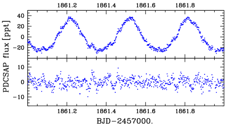
Figure 1: A representative 1-day section of the $TESS$ light curve. Top: original data. Bottom: residuals after removing the orbital frequency and its harmonics.

The $TESS$ data were firstly used to compute the ephemeris of the system. The following equation gives the times of the photometric maxima, when the cool companion is behind the sdB star and shows its heated hemisphere (phase 0.5 in Figure 2). BJD_TDB 2458683.970519 corresponds to the first maximum in the $TESS$ data.

$$BJD_{TDB}=(2458683.970519\,\pm\,0.000035)+$$ (1)

(0.300420467 $\pm$ 0.000000086) E

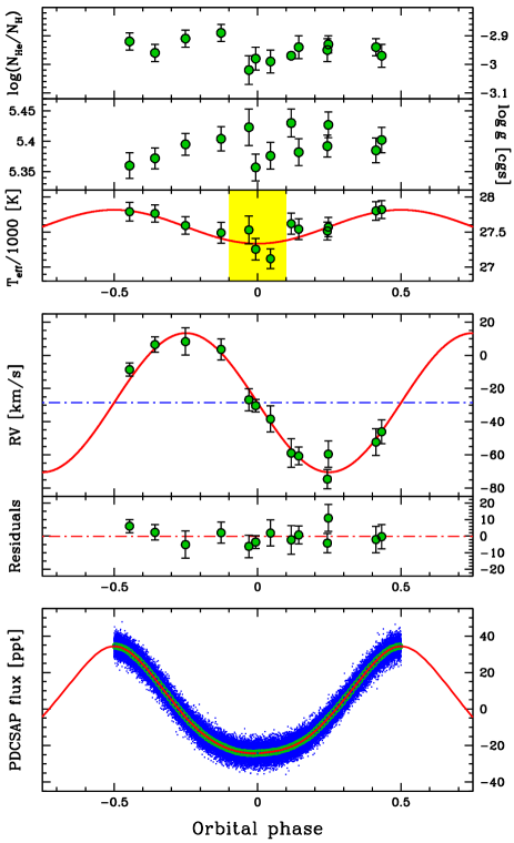
Figure 2: Phase resolved spectroscopy vs photometry of TIC 137608661. Upper panels: He abundance, $\log g$ and $T_{\mathrm{eff}}$ from LTE models as a function of the orbital phase. $T_{\mathrm{eff}}$ shows a clear orbital modulation due to the contribution of the M dwarf companion and for this reason we assume as best $T_{\mathrm{eff}}$ the mean of the three measurements in the phase range –0.1 - 0.1 (yellow rectangle), when the contribution of the secondary star is minimum. Middle panels: radial velocities of the sdB star and residuals. Lower panel: single $TESS$ data (blue dots), mean data in 100 phase bin (green open dots) and best fit (red). Note that the orbital modulation is not perfectly sinusoidal and indeed the fit was performed using also the threee harmonics listed in Table 3. Like in other sdB+dM systems, this behaviour may depend on the values of the various parameters that describe the so-called reflection effect (see e.g. Budaj 2011 for a detailed approach).

3 Low-resolution spectroscopy: Radial Velocities and LTE vs non-LTE sdB atmospheric parameters

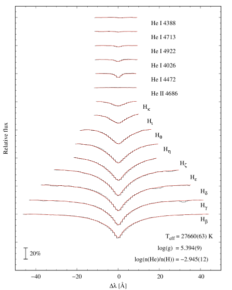
Figure 3: LTE fit to the mean orbit-corrected spectrum obtained from all the thirteen ALFOSC spectra.

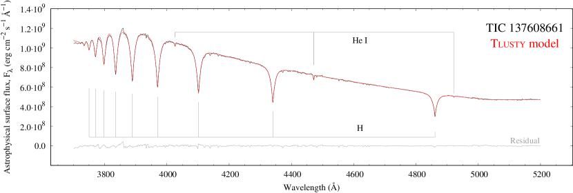
Figure 4: Best-fitting Tlusty/XTgrid non-LTE model (red) to the mean orbit-corrected spectrum obtained from all the thirteen ALFOSC spectra (black). The observed spectrum has been adjusted to the continuum of the final theoretical model. The vertical scale corresponds to the theoretical stellar surface flux based on the model.

Thirteen low-resolution (R$\simeq$2000) spectra of TIC 137608661 were obtained at the Nordic Optical Telescope (NOT, La Palma) using ALFOSC, 250 s exposure times, grism#18, 0.5 arcsec slit, and CCD#14, giving a resolution of 2.2 Å and an approximate wavelength range 345-535 nm. The spectra were homogeneously reduced and analysed. Standard reduction steps within IRAF include bias subtraction, removal of pixel-to-pixel sensitivity variations, optimal spectral extraction, and wavelength calibration based on helium arc-lamp spectra. The peak signal-to-noise ratio of the individual spectra ranges from 80 to 250.

The spectra were taken at different orbital phases and the radial velocities (RVs) were measured using the lines H$\beta$, H$\gamma$, H$\delta$, H8 and H9 through a cross-correlation analysis in which we used as a template a synthetic fit to an orbit-corrected average (all spectra were shifted to zero velocity before averaging). Since the RVs obtained from the last six spectra, all taken on the same night, showed a positive offset respect to the previous measurements, we applied to them a correction of –19.3 km/s. This number was obtained by minimizing the residuals of a least-squares fit. Then we computed a Fourier transform of the RVs, we selected the highest peak, and we optimized the period with a least-squares fit, obtaining an orbital period of 0.30058$\pm$0.00016 d, in good agreement with the photometric orbital period given in equation 1 (previous section). Since the photometric period is much more precise, we then used the latter to optimize RV amplitude and system velocity. We obtain a RV amplitude $K$=41.9$\pm$1.3 km/s and a system velocity $v$=–28.6$\pm$1.2 km/s. The radial velocity fit is shown in the central panels of Figure 2.

After determining the orbital RV amplitude, we shifted the spectra to the system frame of rest, and computed a mean spectrum using all the thirteen spectra. The mean spectrum reaches a peak S/N of $\sim$540 in the region 4725 – 4785 Å. We then used this mean spectrum to determine the physical parameters of the target through spectroscopic model fitting.

We first did a fit using the same H/He LTE grid of Heber et al. (2000) for consistency with earlier studies. We used all the Balmer lines from $H\beta$ to $H\kappa$, as well as the five strongest He i lines for the fit. The LTE fit resulted in values of $T_{\mathrm{eff}}$ = $27660\pm$64 K, $\log g$ = $5.394\pm 0.009$, log${\rm(N_{He}/N_{H})}$ = $-2.945\pm 0.012$. The errors listed on the measurements are the formal errors of the fit, which reflect only the signal-to-noise ratio of the mean, and not any systematic effects caused by the assumptions underlying those models. The best fit of the mean spectrum is shown in Figure 3.

Then, as a next step, we performed a fit of each individual spectrum in order to measure the variations of the atmospheric parameters as a function of the orbital phase, which are shown in Figure 2, together with RVs and $TESS$ photometric data. Since $T_{\mathrm{eff}}$ shows a clear orbital modulation due to the contribution of the M dwarf companion, we assume as best $T_{\mathrm{eff}}$ the mean of the three measurements near phase 0, when the secondary star stands in front of the sdB primary and its contribution is minimum. Instead, for $\log g$ and log${\rm(N_{He}/N_{H})}$, we use the mean of all 13 measurements. Our best values for the sdB atmospheric parameters are: $T_{\mathrm{eff}}$=$27300\pm$200 K, $\log g$=$5.39\pm$0.04, log${\rm(N_{He}/N_{H})}$=$-2.95\pm 0.05$.

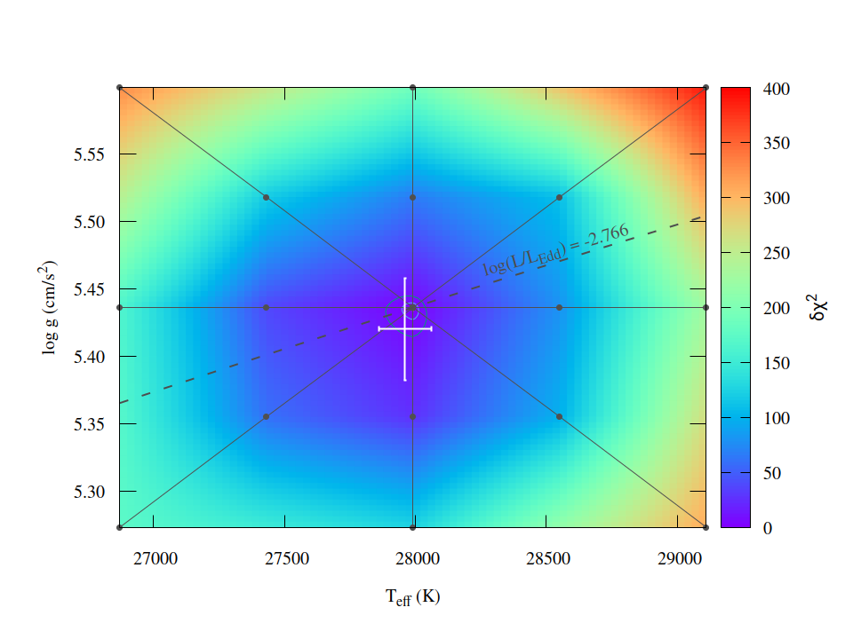
Figure 17: Non-LTE $T_{\mathrm{eff}}$–$\log g$ correlation and two dimensional error determination for TIC 137608661. The color bar shows the chi-square variations with the parameters. The contours are for 60, 90 and 99% confidence intervals and the white error bars represent the adopted final errors.

To determine the atmospheric parameters of TIC 137608661 in non-Local Thermodynamic Equilibrium (non-LTE), we fitted the co-added ALFOSC spectrum with synthetic spectra calculated from Tlusty models (v207; Hubeny & Lanz 2017; Lanz & Hubeny 2007). The models include opacities from H, He, C, N, O, Ne, Mg, Si, and Fe. The spectral analysis was done with a steepest-descent spectral analysis procedure, implemented in the XTgrid code (Németh et al., 2012). The procedure is a global fitting method that simultaneously reproduces all line profiles with a single atmosphere model. XTgrid calculates new model atmospheres and corresponding synthetic spectra iteratively in the direction of decreasing chi-squares. The synthetic spectra are normalized in 80 Å sections to the observation to reduce the effects of the uncalibrated continuum flux on the parameter inference. Figure 4 shows the best-fit non-LTE model to the mean ALFOSC spectrum. The best-fit is obtained when the relative changes of all model parameters decrease below 0.5%. Next, error calculations are performed: while for He abundances the error bars are evaluated in one dimension, for $T_{\rm eff}$ and $\log{g}$ error calculations are performed by mapping the chi-square surface around the best fit as in Figure 17.

The spectroscopic parameters obtained from LTE and non-LTE models are summarized in Table 1. The error bars are statistical. Systematic errors can be estimated from the differences between the two independent analyses. While the surface gravity and helium abundance agree within error bars, the effective temperature is slightly higher in the non-LTE analysis. This difference may partially arise from the fact that in the LTE analysis we used only three spectra close to phase zero, while in non-LTE we used all the spectra since the orbital modulation of $T_{\mathrm{eff}}$ could not be measured, most likely because the global fitting procedure smears out these effects.

Table 1: Spectroscopic parameters, LTE vs non-LTE models.

Parameter	LTE	non-LTE
$T_{\rm eff}$ (K)	27300$\pm 200^{1}$	27960$\pm 100^{2}$
$\log{g}$ (cm s-2)	$5.39\pm 0.04$	$5.42\pm 0.04$
$\log{n{\rm He}/n{\rm H}}$	$-2.95\pm 0.05$	$-2.89\pm 0.05$
1 From only 3 spectra near orbital phase 0.
2 From all 13 spectra. See text for more details.

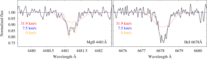
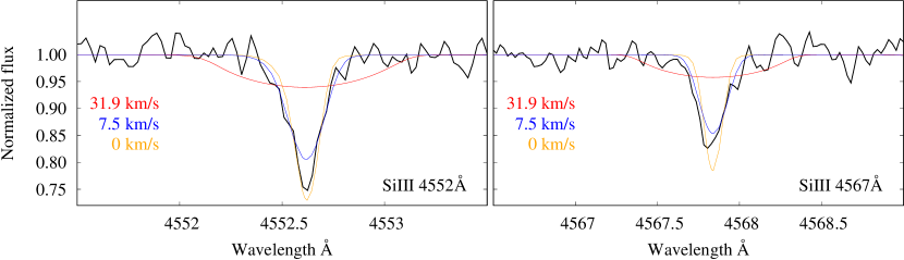
Figure 5: Line fits to the Mg ii 4481 Å, He i 6678 Å, Si iii 4552 Å and Si iii 4567 Å lines with different projected rotation velocities. A synchronous rotation with the binary orbit at $V_{\rm e}\sin{i}=31.9$ km/s (assuming $R$ = 0.209 R_⊙ and an inclination of 65$\degr$, see section 5 and 6.2) can be ruled out. A rigid stellar rotation at $\sim$2.1 km/s (from P_rot=4.6 d, see section 6.2) is not represented since the line profiles would be hardly distinguishable from the zero-rotation profiles. The fit for the entire HERMES spectrum is shown in Figure 18.

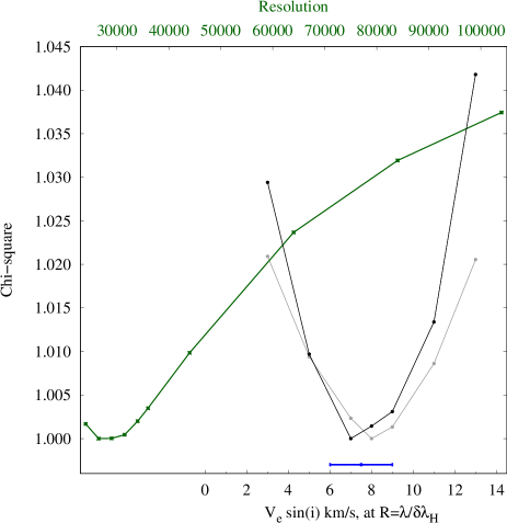
Figure 6: Chi-square values with respect to the projected equatorial rotation velocity (bottom axis). The black curve is based on the lines in Figure 5 and the grey curve is for all selected regions containing metal line in the HERMES spectrum (see Table 5). Both curves show the same minimum, where the blue error bar represents our adopted final value. The green curve shows chi-square values at different resolutions (top axis) and zero rotation. It confirms that there is an extra broadening in the spectrum and the line profiles cannot be reproduced by instrumental broadening alone. The observed broadening due to projected rotation corresponds to an instrumental profile of $R\approx 30\,000$.

4 High-resolution spectroscopy: sdB surface rotation and metal abundances

In order to complement our seismic internal rotation determination described in section 6.2, and try to measure (or at least to put an upper limit to) the rotation rate at the surface of the star from the rotational line-broadening $V_{\rm e}\sin{i}$ of TIC 137608661, we obtained 64 high-resolution spectra, R=85000, using the HERMES instrument (Raskin et al., 2011) at the Mercator telescope. The spectra were obtained from 2021-05-07 to 2021-06-06 with an exposure time of 600 s. We used the wavelength- and barycentric corrected, cosmic-ray clipped, order-merged HERMES-pipeline product.

As the orbital radial velocity varies during the exposures, only observations near the RV minima or maxima at orbital phases 0.25 and 0.75 (see Figure 2) have minimal orbital broadening, which is essential for our attempt to measure $V_{\rm e}\sin{i}$. Therefore we used our TESS ephemeris (equation 1) to predict the best times to acquire the spectra. We obtained 18 spectra close to the orbital phase of RV minimum, and 15 spectra close to the orbital phase of RV maximum. We co-added these 33 spectra after shifting them to remove the orbital RV variation, and we had to apply K=42.26 km/s and a system velocity of -28.41 km/s in order to minimise the velocity difference between the co-added orbit-corrected spectra. These values are in very good agreement with the orbital solution found in section 3 from the ALFOSC@NOT spectra.

The 33 selected spectra have S/N between 4.5 and 11.7; their orbital phase at mid-exposure falls in the ranges 0.2162–0.2806 or 0.7147–0.7849 (using our TESS ephemeris), and the RV variation during the exposures, according to our orbital solution, is less than 1.35 km/s, which is much smaller than the instrumental broadening of FWHM$\sim$3.5 km/s. After co-adding these well-selected 33 orbit-corrected spectra, we reach a continuum peak-S/N around 50. The useful wavelength range is 3900–8950 Å, while the bluest and reddest discernible sharp features are CaII $\lambda$3934 Å and HeI $\lambda$7065 Å.

We fitted the co-added HERMES spectrum using XTgrid for abundances and $V_{\rm e}\sin{i}$. For the wavelength dependent dispersion of the spectrograph we used $\delta\lambda_{H}=0.0087+9.762\times 10^{-6}\,\lambda$, as empirically derived from the width of the ThAr lines in an extrated ThAr spectrum.

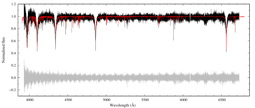
Figure 18: Fit (and residuals) of the entire HERMES spectrum using XTgrid. The wavelength ranges used to determine the surface rotation velocity are specified in Table 5.

Figure 5 shows fits to selected metal lines at two different projected rotation velocities and with zero rotation for reference. The fit for the entire HERMES spectrum can be seen in Figure 18. Our models show that a rotation synchronized with the orbit, corresponding to 31.9 km/s (assuming $R$ = 0.209 R_⊙ and $i$=65$\degr$, see section 5 and 6.2), can be ruled out. However, we find that our models best describe the data for $V_{\rm e}\sin{i}$ $\simeq$ 7.5 km/s. Due to variations in the S/N ratio and continuum placement, the individual lines in Figure 5 do not reflect the projected rotation well. Therefore we selected regions of the spectrum containing sharp metal lines, that are the most sensitive for rotational broadening. These regions are listed in Table 5. Repeating the analysis for these regions confirm a clear minimum in chi-square corresponding to $V_{\rm e}\sin{i}=7.5\pm 1.5$ km/s, as shown in Figure 6. Considering that part of the line broadening may be caused also by other phenomena like instrumental broadening, orbital smearing, micro and macro turbulence, this value should be considered as an upper limit. Among these phenomena, macro turbulence caused by pulsations should be a minor effect. Indeed, g-mode pulsations in sdB stars produce typical RV variations of less than 1 km/s (Silvotti et al., 2020). In HD 4539, that has pulsation amplitudes of the main peaks very similar to TIC 137608661, the RV variations do not exceed 200-300 m/s (Silvotti et al., 2019). Also microturbulence is expected to be small in sdB stars: it was constrained to $\lesssim$ 2 km/s in HD 188112 (Latour et al., 2016, although HD 188112 is a peculiar low-mass sdB, quite different from TIC 137608661). In conclusion our analysis suggests a differential rotation for TIC 137608661, with the envelope rotating faster than the core at a projected rotation velocity not higher than 7.5 km/s. A rigid rotation of the star, which would imply a projected rotation velocity of $\sim$2.1 km/s (from $R$= 0.209 R_⊙, P_rot=4.6 d, $i$=65$\degr$, see section 5 and 6.2) appears unlikely but can not be completely excluded.

The fitting procedure includes all lines from the Synspec line list that show up in the spectrum, which contribute to the fit based on the strength of each line and the S/N ratio of the observation at that wavelength. Table 2 lists metal abundances derived from the HERMES spectrum. The quoted errors are statistical only, calculated in one dimension by mapping the chi-square around the best fit. The measured metal abundances agree with the observed abundance pattern in sdB stars, for which light metals are typically sub-solar while iron is near the solar value (Geier, 2013).

Table 2: Surface metal abundances from high-resolution HERMES spectra and non-LTE models. Solar abundance fractions are given with respect to (Asplund et al., 2009).

Element	$\log{n{\rm X}/n{\rm H}}$	$\log{\epsilon/\epsilon_{\odot}}$
C	$-4.44\pm 0.16$	-0.74
N	$-4.49\pm 0.03$	-0.29
O	$-4.44\pm 0.08$	-1.20
Ne	$-4.29\pm 0.25$	-0.28
Mg	$-5.23\pm 0.11$	-0.72
Si	$-5.54\pm 0.12$	-1.16
Fe	$-4.30\pm 0.20$	0.39

5 Spectral Energy Distribution

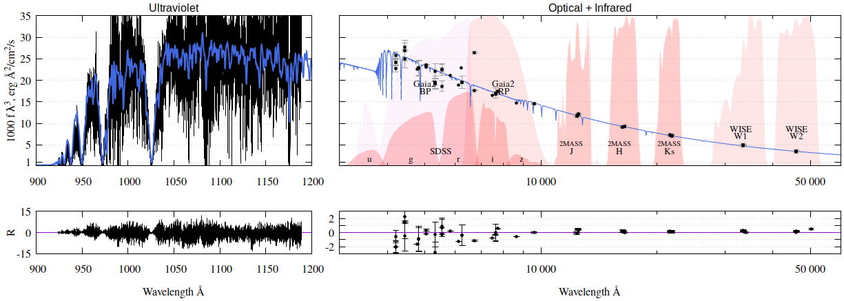
Figure 7: Spectral energy distribution of TIC 137608661 from the far-ultraviolet (FUSE spectrum, left) to the optical and infrared (WISE, right). All photometric data points were taken from the VizieR data service and dereddened for $E(B-V)=0.017$ mag. The shaded regions mark various filter pass-bands. The figure shows the qualitative match between our final spectral model and broadband photometry. The synthetic spectrum was normalized to the observations in the WISE W1 band (33500Å). The SED shows that the FUSE spectrum along with the photometric measurements are consistent with a single stellar component.

Spectral energy distributions (SED) provide a way to evaluate the contributions of binary members to the observed flux. Hot subdwarf stars with F- or G-type companions can be described with two components, which contribute nearly equally to the observed flux in the optical. Late K- and M-type companions remain nearly invisible next to a hot subdwarf. The only exceptions are those in close orbits, when the irradiation by the hot subdwarf is able to form a hot spot on the companion. The strength of irradiation depends on the radii of the components, their separation, as well as the temperature and the spectral properties of the irradiating star (see e.g. Morris & Naftilan 1993 for a simple analytical model). In TIC 137608661 the amplitude of the reflection effect is relatively low, only $\sim$6% (57.5 ppt) when we consider the total amplitude, i.e. the difference between maximum and minimum flux. In HW Vir and NY Vir this contribution is about 20% in the optical, but a precise spectral characterization of the cool companion is still difficult, while in the sdO+dM binary AA Dor it was possible (Vučković et al., 2016) despite the reflection effect amplitude is only $\sim$7%.

For a SED analysis XTgrid collects photometric data from the VizieR Photometry Viewer around 2 arcseconds of the target and shifts the synthetic SED calculated from the spectral modeling to the photometric data. The interstellar extinction toward TIC 137608661 is low, $E$ ($B$–$V$) = 0.017 mag (Schlafly & Finkbeiner, 2011). Figure 7 shows that the match over the optical and infrared regions is excellent and the SED can be modeled with a single hot component. However, a cool ($T_{\rm eff}\lesssim 4000$ K) M dwarf can remain invisible in the SED. The ultraviolet region is very important because the SED of the subdwarf peaks there. The only measurement from GALEX is significantly off, most likely due to the bright non-linearity of the GALEX photometry (Morrissey et al., 2007). Fortunately, there are FUSE observations of the star (e.g.: FUSE Program ID: G061, PI: Pierre Chayer), which confirm the far-UV flux level (left panels of Figure 7).

With an independent distance measurement provided, the SED analysis returns radius, luminosity and mass of the hot subdwarf. We used the Gaia EDR3 distance $d$ = 256.5 $\pm$ 2.6 pc and found an angular diameter $\log{\theta}$ =–10.434 $\pm$ 0.070 rad for the sdB in TIC 137608661, which results in a stellar radius $R$ = 0.209 $\pm$ 0.005 R_⊙. Then, adopting $T_{\mathrm{eff}}$=27960 K and $\log g$=5.42 from non-LTE results, we obtain $L$ = 23.98 $\pm$ 1.09 L_⊙ and $M$ = 0.419 $\pm$ 0.041 M_⊙.

Following Deca et al. (2012), the $B$–$V$ = – 0.37 and $J$–$K_{s}$ = – 0.187 mag color indices suggest a very low contribution from the companion, indicating that it must be a low-mass main sequence star. A white dwarf companion is excluded since it would not give rise to the reflection effect that we see in TESS data, while it would produce ellipsoidal variations which are not detected. Moreover, from the binary mass function, a WD companion would imply an inclination of the system lower than $\sim$15$\degr$, which is not compatible with the inclination of (65${}^{+10}_{-20}$)$\degr$ found from the seismic analysis in section 6.2. Further spectral characterization of the companion would require high SNR infrared spectroscopy.

6 SdB pulsations

6.1 Fourier analysis

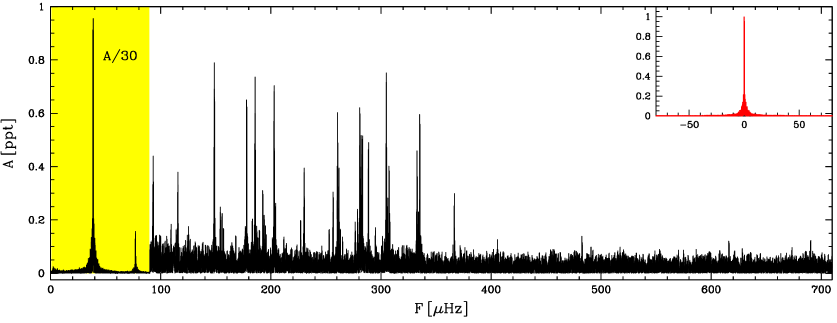
Figure 8: Amplitude spectrum of TIC 137608661 using all three sectors together. The yellow section corresponds to the orbital frequency and its first harmonic. The upper-right inset is the window function (in red).

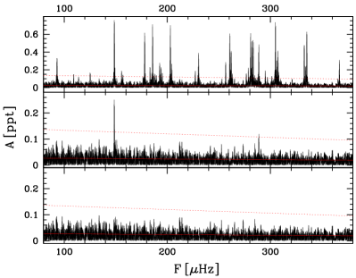
Figure 9: Prewhitening procedure. Upper panel: spectrum of TIC 137608661 in the main pulsation region. Central panel: residuals after having removed 55 significant peaks. Bottom panel: residuals after having removed also f6b and f33b. The solid red line and the dotted red line are the mean noise level and the 5$\sigma$ detection threshold, respectively. See text for more details.

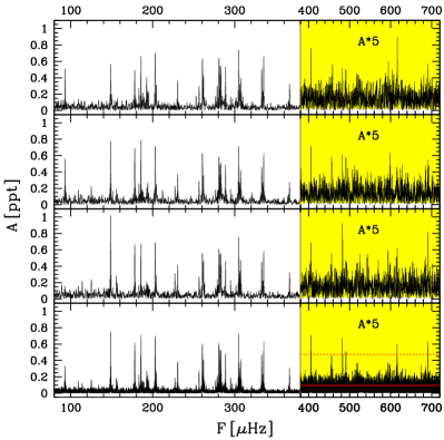
Figure 10: Amplitude spectrum of each single sector. From top to bottom: sector 14, 20, 26 and all three sectors together. Like in Figure 9, the solid red line and the dotted red line are the mean noise level and the 5$\sigma$ detection threshold, respectively.

The Fourier transform (FT) of the $TESS$ data in Figure 8 shows a rich spectrum. The low-frequencies are dominated by the orbital modulation at 38.526 $\mu$Hz, with an amplitude of 28.77 ppt, plus its harmonics at 77.052, 115.578 and 154.105 $\mu$Hz. As expected, these harmonics have decreasing amplitudes: 4.74, 0.42 and 0.26 ppt respectively. A fourth harmonic at 192.645 $\mu$Hz has an amplitude of 0.27 ppt, higher than expected, and indeed, as we will see, this frequency is also part of a triplet of pulsation frequencies, suggesting that a tidal-induced mechanism might be at work in this case. Resonance between tides and g-modes pulsations is predicted by theory (Zahn, 1975, 1977; Preece et al., 2018) and may have been seen in a few sdB pulsators (e.g. Reed et al. 2011; Silvotti et al. 2014).

At frequencies higher than 90 $\mu$Hz, up to $\sim$370 $\mu$Hz, many peaks with amplitudes of several hundreds of ppm (part per million) correspond to a typical sdB spectrum of g-mode pulsations. A few lower-amplitude peaks ($\sim$100 ppm) are present also at higher frequencies, up to 690 $\mu$Hz.

To define a reliable noise threshold we proceeded as follows. First we computed the signal-to-noise ratio (S/N) corresponding to a False Alarm Probability (FAP) of 0.1$\%$ following Kepler (1993): S/N=ln(n_f*1000)^0.5 in which n_f=F_N/R_f is the number of independent frequencies, F_N is the Nyquist frequency, R_f=1/$\Delta$T is the nominal frequency resolution and $\Delta$T is the total duration of the run. We obtain S/N=4.5. Then, to test the reliability of this number, we computed the FT of 1000 simulated light curves obtained by reshuffling in a random way the data, after having removed 57 significant frequencies (those in Table 3). Since reshuffling destroys any coherent signal, the S/N ratio of the highest peak of each FT was used to test the previous S/N expression. We found that the expression is valid as long as an offset is used and this offset is independent from the number of simulations suggesting that it is robust. For this data set the offset on S/N is +0.5 or +0.8 depending whether we use the FT mean noise or the FT median noise as the denominator. These numbers are very similar to those found by Baran & Koen (2021) in their simulations. In conclusion, using the FT mean noise, we adopted S/N=5.0 as our threshold for real pulsation frequencies, while the peaks with 4.5$<$S/N$<$5.0 are considered as candidates only. Once the signal-to-noise threshold has been set, we must consider that the mean noise is not constant everywhere. Since it is flat at high frequencies but tends to increase at low frequencies (due to low-amplitude peaks, below the threshold, unresolved peaks, aliasing effects, etc., which are not removed by prewhitening), after some measurements in different frequency intervals we decided to adopt a noise model which is linearly decreasing between 90 and 380 $\mu$Hz (0.027 ppt at 90 $\mu$Hz and 0.019 ppt at 380 $\mu$Hz) and remains constant at 0.019 ppt up to 700 $\mu$Hz.

We applied to the light curve a standard prewhitening procedure with nonlinear least-squares fitting and obtained a list of frequencies that is shown in Table 3. Those with S/N between 4.5 and 5.0, that are considered as candidates only, are marked with parentheses in Table 3. The prewhitening procedure is illustrated in Figure 9. After prewhitening, only two frequencies were not completely removed from the amplitude spectrum (central panel of Figure 9), leaving residuals that could be due either to pairs of very close frequencies below the frequency resolution, or to frequency instability (frequencies and/or amplitudes that vary over time).

When we compare the amplitude spectra of the various sectors (Figure 10), we see that most peaks are rather stable in amplitude, despite the fact that from one sector to another there are about six months, for a total duration of the observations of about one year.

Table 3: Orbital and pulsation frequencies.
(Errors in brackets are relative to the last digits, e.g. 38.526250 (11) means 38.526250$\pm$0.000011).

ID	F ($\mu$Hz)	P (s)	A (ppt)	S/N	n1	$l$	m
forb	38.526250 (11)	25956.3283 (72)	28.774 (17)
2*forb	77.052472 (65)	12978.169 (11)	4.738 (17)
3*forb	115.57770 (73)	8652.188 (55)	0.420 (17)
4*forb	154.1055 (12)	6489.062 (50)	0.261 (17)
f1	93.0623 (10)	10745.49 (12)	0.297 (17)	11.0
f2	93.15969 (99)	10734.26 (11)	0.311 (17)	11.6
f3	109.3401 (21)	9145.78 (18)	0.144 (17)	5.4
(f4	114.0211 (25)	8770.31 (19)	0.123 (17)	4.7)
f5	125.1936 (19)	7987.63 (12)	0.162 (17)	6.2
f6	148.63137 (40)	6728.055 (18)	0.764 (17)	30.1	26	1?	+1?
f6b2	148.6551 (12)	6726.982 (56)	0.249 (17)	9.8
f7	155.6834 (17)	6423.292 (71)	0.179 (17)	7.1	25	1	0?
f8	156.9764 (23)	6370.385 (92)	0.136 (17)	5.4	25	1	+1?
f9	178.03636 (49)	5616.830 (16)	0.622 (17)	25.3	22	1?	+1?
f10	183.2003 (17)	5458.506 (50)	0.183 (17)	7.5	21	1	-1
f11	185.69940 (43)	5385.047 (13)	0.710 (17)	29.1	21	1	+1
f12	188.3160 (20)	5310.222 (57)	0.152 (17)	6.3
f13	189.5612 (22)	5275.343 (62)	0.137 (17)	5.6
f14	192.6449 (11)	5190.898 (31)	0.270 (17)	11.2	20	1	-1
f15	193.9138 (14)	5156.930 (37)	0.223 (17)	9.2	20	1	0
f16	195.1421 (19)	5124.472 (50)	0.162 (17)	6.7	20	1	+1
f17	203.00214 (44)	4926.056 (11)	0.693 (17)	29.0	19	1	-1?
f18	204.2614 (12)	4895.688 (29)	0.257 (17)	10.8	19	1	0?
f19	227.0400 (17)	4404.510 (32)	0.185 (17)	8.0		2?
(f20	227.2388 (27)	4400.657 (53)	0.113 (17)	4.9)
f21	230.30385 (78)	4342.090 (15)	0.392 (17)	16.9	17	1	+1?
(f22	252.9085 (30)	3953.999 (46)	0.104 (17)	4.6)
f23	256.6026 (12)	3897.077 (18)	0.265 (17)	11.8		2?
f24	260.61413 (52)	3837.0905 (77)	0.591 (17)	26.5	15	1	-1
f25	261.2016 (21)	3828.461 (30)	0.150 (17)	6.7		2?
f26	261.86840 (70)	3818.712 (10)	0.440 (17)	19.8	15	1	0
(f27	263.1036 (29)	3800.785 (42)	0.105 (17)	4.7	15	1	+1)
f28	276.5385 (22)	3616.134 (28)	0.142 (17)	6.5		2
f29	278.6794 (14)	3588.353 (18)	0.221 (17)	10.1		2
f30	280.75348 (51)	3561.8436 (65)	0.601 (17)	27.6	14	1	-1
f31	282.00815 (58)	3545.9968 (73)	0.530 (17)	24.4	14	1	0
f32	283.23899 (57)	3530.5874 (71)	0.540 (17)	24.9	14	1	+1
f33	288.68769 (65)	3463.9510 (79)	0.470 (17)	21.8		2?
f33b3	288.7149 (25)	3463.624 (30)	0.122 (17)	5.7
f34	294.9645 (16)	3390.238 (19)	0.188 (17)	8.8		2	-1 or -2
f35	297.0378 (25)	3366.575 (28)	0.122 (17)	5.7		2	0 or -1
f36	301.3289 (29)	3318.632 (31)	0.108 (17)	5.1		2	+2 or +1
f37	304.84395 (40)	3280.3669 (43)	0.764 (17)	36.3	13	1	-1
f38	306.1024 (11)	3266.880 (11)	0.288 (17)	13.7	13	1	0
f39	307.33246 (65)	3253.8053 (69)	0.472 (17)	22.5	13	1	+1
(f40	320.8888 (31)	3116.344 (30)	0.099 (17)	4.8		2?)
f41	332.78156 (70)	3004.9742 (63)	0.439 (17)	21.6	12	1	-1
f42	334.0450 (15)	2993.608 (13)	0.211 (17)	10.4	12	1	0
f43	335.27579 (52)	2982.6192 (46)	0.595 (17)	29.4	12	1	+1
(f44	365.4018 (32)	2736.714 (24)	0.095 (17)	4.9	11	1	0?)
f45	366.69996 (99)	2727.0251 (74)	0.311 (17)	16.1	11	1	+1?
f46	405.9003 (22)	2463.659 (13)	0.142 (17)	7.5	10	1	-1?
(f47	456.0976 (34)	2192.513 (16)	0.091 (17)	4.8	9	1	-1?)
f48	482.5889 (23)	2072.157 (10)	0.132 (17)	6.9
f49	490.8909 (30)	2037.113 (13)	0.102 (17)	5.4
f50	616.0114 (26)	1623.3466 (68)	0.119 (17)	6.3	7	1	+1?
f51	690.3358 (25)	1448.5704 (52)	0.124 (17)	6.5
1 Arbitrary offset. Assuming that the period spacing is constant, we consider n=1 for the
shortest period.
2 Residual (unresolved) peak after removing f6. See text for more details.
3 Residual (unresolved) peak after removing f33. See text for more details.

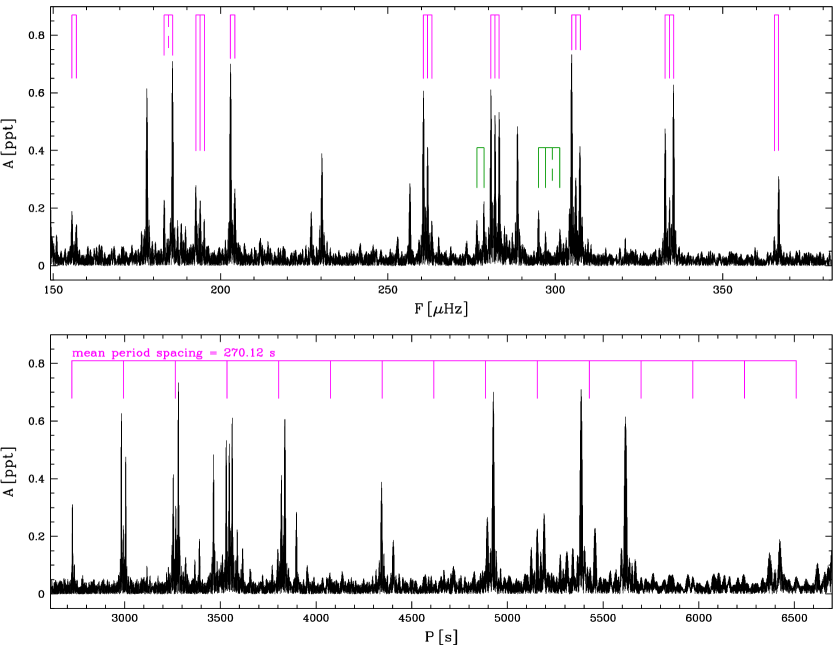
Figure 11: Frequency splitting (top) vs period spacing (bottom). Magenta refers to $l$=1 modes while green refers to $l$=2. Both panels represent exactly the same region of the spectrum.

6.2 Period spacing, frequency splitting, inclination of the rotation axis

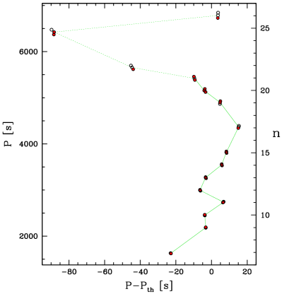
Figure 12: Échelle diagramme of the dipole modes showing the residuals between observed periods and theoretical periods computed assuming a constant period spacing of 270.116 s. The open circles are the missing components of the rotational triplets.

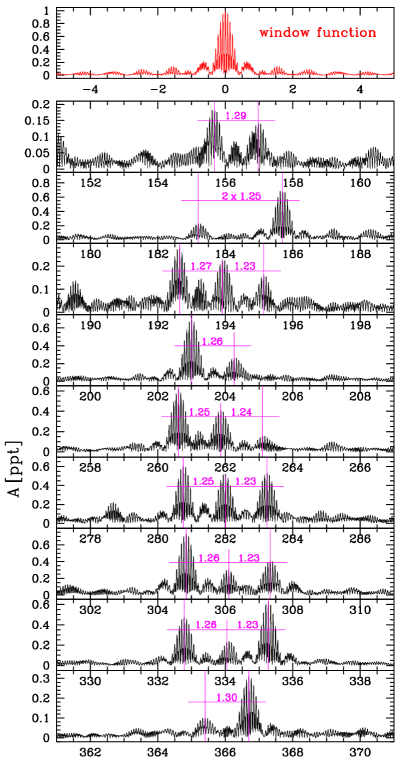
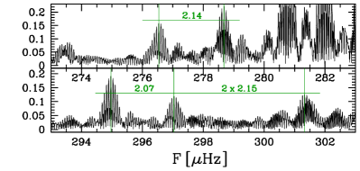
Figure 13: Frequency splitting in detail: the nine complete or incomplete $l$=1 triplets and the two incomplete $l$=2 quintuplets.

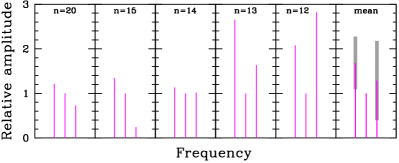
Figure 14: Relative amplitudes of the components of the five $l$=1 triplets. The amplitude of the central component of each triplet is normalized to 1 before computing the mean amplitudes, which are shown in the rightmost panel. The error bars (in grey) are the standard deviations around the mean amplitudes.

Looking at the amplitude spectrum of TIC 137608661, we immediately note four consecutive triplets of equally spaced frequencies between $\sim$260 and $\sim$340 $\mu$Hz with a frequency spacing of about 1.3 $\mu$Hz (Figure 11 upper panel). Another triplet located near $\sim$190 $\mu$Hz and a few doublets between $\sim$150 and $\sim$370 $\mu$Hz show a very similar frequency spacing. When we plot the same region of the spectrum in the period domain (lower panel of Figure 11), we see that the central peaks of the four well defined triplets between 260 and 340 $\mu$Hz are equally spaced in period. The period difference between the central peaks at 3818.7, 3546.0, 3266.9 and 2993.6 s is 272.7, 279.1 and 273.3 s respectively, confirming that the triplets are consecutive $l$=1 modes. The mean period spacing of these four triplets is 275.03 s. Since the central peak of the triplet near $\sim$190 $\mu$Hz, which has a period of 5156.9 s, is also well compatible with the $l$=1 sequence of modes, we include also this period in the computation of the mean period spacing. From a linear least-squares fit to the five $m$=0 periods we obtain $\Delta$P$=270.12\pm 1.19$ s. Using this value, several other doublets fall close to the expected periods (assuming a perfectly constant spacing) and therefore we adopt 270.12 s in our analysis. Once the period spacing is fixed, we were able to identify further modes, including a few $l$=1 single peaks at short and long periods. The geometry of the identified modes (number of radial nodes n, spherical degree $l$, and azimuthal quantum number m) is reported in Table 3. In Figure 12 the “échelle diagramme” of the $l$=1 sequence shows the residuals between observed and theoretical periods. We note the typical meandering shape between $\sim$2000 and $\sim$5000-6000 s that is also seen in other sdB pulsators such as KIC 10553698A (Østensen et al., 2014b), EPIC 211779126 (Baran et al., 2017), KIC 10001893 (Uzundag et al., 2017), KIC 11558725 (Kern et al., 2018), PHL 457 (Baran et al., 2019). And we see that the periods at n=22 (f9) and n=25 (f7 and f8) are significantly shorter than the expected values from a constant period spacing, indicating a possible mode trapping. Although an incorrect identification as dipole modes can not be totally excluded, the frequency difference between f7 and f8, equal to 1.29 $\mu$Hz, suggests that f7 and f8 are indeed two components of the same $l$=1 triplet.

Figure 13 shows all the complete or incomplete $l$=1 triplets of frequencies split by the rotation of the star. Considering all of them, we obtain a mean frequency splitting of 1.254 $\mu$Hz corresponding to a rotation period of about 4.6 days in the deep layers of the star.
The rotation period is obtained from the expression P_rot=(1–C_nl)/$\delta\sigma_{nl}$ (where $\delta\sigma_{nl}$ is the frequency spacing), which is valid for a slowly rotating star with $\Omega_{\rm rot}<<\sigma_{\rm puls}$. For high-order g-modes, in the asymptotic limit, we can use the following approximation: C_n,l $\simeq$ 1/[($l$ ($l$+1)] and we obtain C_(l=1)$\simeq$1/2 and C_(l=2)$\simeq$1/6 (Ledoux, 1951; Unno et al., 1989; Aerts et al., 2010). Although a sequence of $l$=2 equally spaced periods is not seen in our data, from the $l$=1 splitting of 1.254 $\mu$Hz we can compute the expected frequency splitting for the $l$=2 modes: $\delta\sigma_{(l=2)}$ $\simeq$ $\frac{5}{3}\,\delta\sigma_{(l=1)}$$\simeq$ 2.090 $\mu$Hz. And indeed we see two multiplets of frequencies (a doublet and a triplet) which have frequency separations very close to this number. These incomplete quintuplets are shown in the lower panels of Figure 13 and are reported in Table 3. The $l$=2 spherical degree has been tentatively attributed also to a few other frequencies.

There is another valuable piece of information that can be derived from the very clean amplitude spectrum of TIC 137608661. Having a certain number of clearly identified $l$=1 triplets, we can analyze the amplitude of each m-component to derive an estimate of the inclination of the rotation axis respect to the line of sight. More precisely, the geometric visibility of each m-component, and therefore its amplitude, depends on the angle between the pulsation axis and the line of sight. However, misalignments between pulsation and rotation axis, which would split each $l$=1 mode in nine components (Pesnell, 1985), have never been seen in sdB stars. Thus we can safely assume that pulsation and rotation axes are aligned. If we also assume that, on average, each m-component of a multiplet receive the same amount of energy and develop approximately the same intrinsic amplitude level, then the mean amplitude ratio between m=$\pm$1 and m=0 components of a certain number of triplets should directly reflect the inclination of the rotation axis. With five well-defined triplets, this measurement should already have some level of accuracy. In Figure 14 we show the relative amplitudes of the components of the five triplets, the mean amplitudes of the m=–1,0,+1 components, and their errors. A comparison between these numbers and those computed by Charpinet et al. (2011, Supplementary Information, Figure A.5; see also ), allows us to exclude low inclinations and suggests an inclination of (65${}^{+10}_{-20}$)$\degr$ for the rotation axis of the sdB star.

With such inclination, and adopting a radius of 0.209 ${\mathrm{R}}_{\odot}$ from the SED analysis (section 5), the projected equatorial rotation velocity near the surface of the star $V_{\rm e}\sin{i}$ = 7.5 km/s obtained in section 4 would correspond to an orbital period of 1.3 days, shorter than the 4.6 days obtained in the deep layers, suggesting a differential rotation, although a rigid rotation can not be totally ruled out as discussed in section 4.

6.3 Asteroseismic analysis

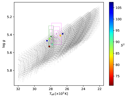
Figure 15: Asteroseismic determination of $T_{\mathrm{eff}}$ and $\log g$. Color coded $S^{2}$ (as defined in equation 2) outlines the best models. Minimum $S^{2}$ is obtained for $T_{\mathrm{eff}}$=28180 K and $\log g$=5.53 (dark-red point). Magenta and dark-green small points/rectangles represent spectroscopic $T_{\mathrm{eff}}$ and $\log g$ with 1, 2 and 3 $\sigma$ error boxes, from LTE and non-LTE models respectively.

In order to obtain more insight about evolutionary status and interior of TIC 137608661, we calculated evolutionary models using the MESA code (Modules for Experiments in Stellar Astrophysics; Paxton et al., 2011; Paxton et al., 2013, 2015, 2018, 2019), version 11701. The models were calculated for progenitors with initial masses, $M_{\mathrm{i}}$, in the range of $1.0\,-\,1.8\,M_{\odot}$, with a step of $0.01\,M_{\odot}$, and metallicities, $Z$, in the range of $0.005\,-\,0.035$, with a step of $0.005$. The initial helium abundance was determined by the linear enrichment law, $\Delta\,Y/\Delta\,Z=1.5$. The protosolar helium abundance, $Y_{\odot,\,\mathrm{protosolar}}=0.2703$, and the mixture of metals were adopted from Asplund et al. (2009). The progenitors were evolved to the tip of the red giant branch where, before the helium ignition, most of the hydrogen has been removed leaving only a residual hydrogen envelope on top of the helium core. The considered envelope masses, M_env, are in the range of $0.0001\,-\,0.0030\,M_{\odot}$, with a step of $0.0001\,M_{\odot}$. The models were then relaxed to an equilibrium state and evolved until the depletion of helium in the core. In all calculations we used the novel convective premixing scheme in order to ensure proper growth of the convective core during the course of evolution (Paxton et al., 2019). The thorough description of the models is provided in Ostrowski et al. (2021). The adiabatic pulsation calculations were performed using the GYRE code, version 5.2 (Townsend & Teitler, 2013; Townsend et al., 2018). The pulsation models were calculated for evolutionary models with central helium abundance, $Y_{\mathrm{c}}$, in the range of $0.9\,-\,0.1$, with a step of $0.05$. The models with $Y_{\mathrm{c}}<0.1$ were not considered due to the occurrence of the breathing pulses, which are unavoidable side effects of the convective premixing scheme (Ostrowski et al., 2021).

The grid of evolutionary models was used to find the models that represent TIC 137608661. No spectroscopic constraints were used in the process and we have chosen to fit only the five pulsation periods corresponding to the m=0 dipole modes identified via multiplet structures (f15, f26, f31, f38 and f42 in Table 3). We used a goodness-of-fit function, which calculates the difference between observed and theoretical periods

$$S^{2}=\frac{1}{N_{\rm o}}\,\sum^{N_{\rm o}}_{i=1}\left(P_{\rm o}^{i}-P_{\rm c}^{i}\right)^{2}$$ (2)

where $P_{\mathrm{o}}$ is an observed period, $P_{\mathrm{c}}$ is a calculated period, and $N_{\mathrm{o}}$ is the number of periods used (5 in this case). The minimum of the $S^{2}$ function indicates the best fit.

Considering only the six best solutions with $S^{2}$ up to about $150\%$ of the minimum $S^{2}$, these best models clearly indicate that the progenitor of TIC 137608661 is a star with a metallicity close to solar, $Z=0.01-0.015$, with a mass $M_{\mathrm{i}}=1.1-1.2\,M_{\odot}$. The estimated age of the star is $5.4-7.3$ Gyr. The envelope mass of the star is constrained in the narrow range $M_{\mathrm{env}}=0.0006-0.0009\,M_{\odot}$. As shown in Figure 15, the best solutions are located close to the spectroscopic determinations of $T_{\mathrm{eff}}$ and $\log\,g$. Such spectroscopic values suggest a rather evolved EHB model, which is supported by the low central helium abundance of the best models, $Y_{\mathrm{c}}=0.3-0.1$.

7 TIC 137608661 in context: synchronized vs non-synchronized sdBs in short-period binaries

Table 4: SdB rotation (from asteroseismology) vs orbital periods.

Name∗	Porb (d)	Prot (d)	Prot (d)	Comments	Ref.
		g-modes	p-modes
$\bullet$ sdB+dM binaries
NY Vir (PG 1336-018)	0.10083		0.10083	rigid rot. down to 0.55 R⋆	(1)
TYC1 4544-2658-1 (TIC 137608661)	0.300	4.6			(2)
PHL 457 (EPIC 246023959)	0.31289	4.6	2.5 ?		(3)
V1405 Ori (EPIC 246683636)	0.39802	4.2 ?	0.555		(4)
B4 in NGC 6791 (KIC 2438324)	0.3985	9.20			(5,6,7)
KIC 11179657	0.394	7.4			(8,6)
KIC 2991403	0.443	10.3			(8,6)
EQ Psc (EPIC 246387816)	0.80083	9.4			(3)
$\bullet$ sdB+WD binaries
HD 265435 (TIC 68495594)	0.0688185		0.069		(9)
KL UMa (Feige 48)	0.34361		0.38	rigid rotation	(10,11)
PG 1142-037 (EPIC 201206621)	0.5411	>45.			(12)
KIC 7664467	1.5590	35.1			(13)
EPIC 211696659	3.16	>28.			(14)
KIC 10553698	3.39	41.			(15)
KIC 11558725	10.05	$\sim$45.	$\sim$40.	$\sim$44 d rigid rotation	(16,17)
FBS 1903+432 (KIC 7668647)	14.17	46-48	49-52 ?	close to rigid rotation	(18)
$\bullet$ sdB+FGK wide binaries
PG 0048+091 (EPIC 220614972)	?	13.9 ?	4.4	sdB+F	(19)
EPIC 211823779	?		11.5 ?	sdB+F1V	(14)
PG 1315-123 (EPIC 212508753)	?	15.8	16.2	sdB+F	(19)
EGGR 266 (EPIC 211938328)	635		21.5 ?	sdB+F6V	(14)
$\bullet$ single sdBs
EPIC 211779126			$\sim$16	core rotation likely slower	(20)
UY Sex (EPIC 248411044)			24.6		(4)
KIC 10139564		$\sim$26	$\sim$26	rigid rotation	(21,22)
KY UMa (PG 1219+534)			34.9	rigid rot. down to 0.6 R⋆	(23)
KPD 1943+4058 (KIC 5807616)		39.2			(24)
KIC 2697388		$\sim$42	$\sim$53	close to rigid rotation	(25,26)
KIC 3527751		42.6	15.3 ?		(27,28)
EPIC 203948264		$\geq$45.9			(29)
TIC 33834484		64			(30)
EPIC 212707862		$\sim$80			(31)
KIC 10670103		88			(32)
KIC 1718290		$\sim$100		BHB star !	(33)
KIC 10001893		289			(34)
∗ Kepler/K2/TESS id are used as 1st or 2nd name when the results are based on Kepler/K2/TESS data.
(1) Charpinet et al. 2008; (2) this paper; (3) Baran et al. 2019; (4) Reed et al. 2020; (5) Pablo et al. 2011;
(6) Baran & Winans 2012; (7) Sanjayan et al. 2022; (8) Pablo et al. 2012; (9) Pelisoli et al. 2021;
(10) orbital period from TESS data preliminary analysis; (11) Van Grootel et al. 2008; (12) Reed et al. 2016;
(13) Baran et al. 2016; (14) Reed et al. 2018b; (15) Østensen et al. 2014b; (16) Telting et al. 2012;
(17) Kern et al. 2018; (18) Telting et al. 2014; (19) Reed et al. 2019; (20) Baran et al. 2017;
(21) Baran et al. 2012; (22) Zong et al. 2016; (23) Van Grootel et al. 2018; (24) Charpinet et al. 2011 (SI);
(25) Baran 2012; (26) Kern et al. 2017; (27) Foster et al. 2015; (28) Zong et al. 2018; (29) Ketzer et al. 2017;
(30) Uzundag et al. in prep.; (31) Bachulski et al. 2016; (32) Reed et al. 2014; (33) Østensen et al. 2012;
(34) Charpinet et al. 2018.

With an orbital period of 7.21 hours, a well defined rotation period of 4.6 days in the deep layers, and a lower limit to the rotation period of about 1.3 days near the surface, the sdB star in TIC 137608661 is relatively far from synchronization. However, among the handful of sdB+dM binaries for which the sdB rotation was measured through asteroseismology, it is the non-synchronized system with both the shortest orbital period and the shortest sdB rotation period. Only PHL 457, with basically the same sdB core rotation period and a slightly longer orbital period of 7.51 hours (Baran et al., 2019), ranks at the same level in the synchronization process. Table 4 shows the list of sdB/sdO stars for which the rotation period was measured from g- or p-mode frequency splitting.

A few stars are not reported in Table 4:
$\bullet$ KIC 2991276 since it is not clear whether this star is single or in a binary system. The short rotation period (6.3 d) measured from p-modes (Østensen et al., 2014a) suggests the presence of a companion and the low amplitude of the m=$-$1,+1 modes belonging to the triplets near 7560 and 8200 $\mu$Hz suggest a low inclination $i$$\stackrel{{\scriptstyle{\displaystyle<}}}{{\sim}}$15$\degr$. A low inclination, together with KIC 2991276’s faintness (17th-mag), means that it is not easy to verify the presence of a companion for this star.
$\bullet$ Also Balloon 090100001 shows a similar rotation period between 6.4 and 7.4 days from p-modes, but in this star the frequency splitting changes in 1 year (Baran et al., 2009). The reasons for this peculiar behaviour are unclear and the presence of a magnetic field with the strength of $\sim$1 kG was excluded by Savanov et al. (2013).
$\bullet$ No rotational splitting was detected in HD 4539/EPIC 220641886 and KIC 8302197 (Silvotti et al., 2019; Baran et al., 2015a), suggesting long rotation periods (too long to be measured respect to the observing runs) and/or low inclinations.
$\bullet$ B3 and B5 in the open cluster NGC 6791 show a mean rotation period of 64.2 and 71 days respectively (the latter somewhat uncertain), for both stars RV variations suggest the presence of a companion, but the orbital periods are unknown (Sanjayan et al., 2022). Interestingly, in B3 the l=1 g-mode frequency splitting decreases at increasing frequencies, suggesting that differential rotation could operate even on a small radius scale.
$\bullet$ No frequency multiplets were found in the amplitude spectrum of 2M 1938+4603, an sdB+dM binary with an orbital period of 3.02 hours (Baran et al., 2015b, and references therein).
$\bullet$ A clear detection of rotational splitting is missing in KPD 1930+2752, an sdB+WD binary with an orbital period of only 2.3 hours that shows ellipsoidal variations (Billéres et al., 2000; Reed et al., 2011).
With such short orbital periods, both the sdB stars in 2M 1938+4603 and KPD 1930+2752 should be synchronized or very close to synchronization.

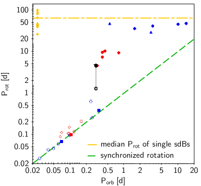
Figure 16: SdB rotation period vs orbital period. Red symbols: sdB+dM systems with sdB rotation period obtained from g-mode or p-mode frequency splitting (filled circles and filled square respectively) or from spectral line broadening (empty circles or empty diamonds, the latter indicating a brown dwarf companion). Black symbols: TIC 033834484, deep-layers rotation period from g-modes frequency splitting (filled asterisk), and lower limit to the surface rotation period from spectral line broadening (empty asterisk). Blue symbols: sdB+WD systems with sdB rotation period obtained from g-mode frequency splitting (filled circles or filled triangles that indicate a lower limit) or p-mode frequency splitting (filled squares) or from spectral line broadening (empty circles). Yellow symbols: single sdB stars with rotation period obtained from g-mode frequency splitting (triangle indicating a lower limit). The seven red empty symbols correspond to the following HW Virginis (eclipsing sdB+dM/BD) systems: from left to right V 2008-1753 (Schaffenroth et al., 2015; Schaffenroth et al., 2021), SDSS J162256.66+473051.1 (Schaffenroth et al., 2014), PTF1 J011339.09+225739.1 (Wolz et al., 2018), HS 0705+6700 (Drechsel et al., 2001), SDSS J082053.53+000843.4 (Schaffenroth et al., 2021), HW Vir (Geier et al., 2010; Baran et al., 2018; Esmer et al., 2021), EPIC 216747137 (Silvotti et al., 2021). The seven blue empty circles correspond to the following non-eclipsing (or partially eclipsing) sdB+WD binaries: from left to right ZTF J2130+4420 (Kupfer et al., 2020a), ZTF J2055+4651 (Kupfer et al., 2020b), CD-30$\degr$11223 (Vennes et al., 2012), PTF1 J0823+0819 (Kupfer et al., 2017), EVR-CB-001 (Ratzloff et al., 2019), PG 2345+318 (Geier et al., 2010; Green et al., 2004), EVR-CB-004 (Ratzloff et al., 2020b).

Focusing on short-period binaries (both sdB+dM and sdB+WD systems), Figure 16 includes also some systems for which the sdB rotation period is inferred from the rotational velocity measured through spectral line broadening: P_rot=2$\pi$R sin $i$/(v sin $i$). This technique is more efficient at very short rotation periods and high equatorial velocities, when the slow-rotation approximation normally used for the rotational splitting may no longer be valid. This might be the reason why we do not see frequency splitting in 2M 1938+4603 and KPD 1930+2752.

We see from Figure 16 that synchronization occurs for orbital periods shorter than $\sim$0.3 days (first group of stars), while at orbital periods longer than $\sim$1 day (second group) the rotation periods are close to the typical values of single stars, of a few tens of days. Between these two groups, a third group is formed by the stars that are approaching synchronization. It is important to note that different methods were used to measure P_rot in these three groups and these methods sample different regions of the star: deep layers with the g-mode frequency splitting used in group 2 and 3, external layers with the spectral line broadening or p-mode frequency splitting used in group 1. Indeed, a few systems in Table 4, for which the sdB rotation was measured at different depths, suggest that differential rotation might be quite common in these stars. And this can partially explain why the jump between group 2 and 3 and group 1 that we see in Figure 16 is so steep.

Figure 16 suggests a few further comments: in group 1 the three systems that have a brown dwarf (BD) companion (represented with red empty diamonds) are not fully synchronized, differently from the other sdB+dM systems with similar orbital periods. Although we do not know their evolutionary phase, this effect may be related to their longer synchronization time which is inversely proportional to the companion mass. At longer orbital periods, the two sdB/sdO+WD systems PG 2345+318 and EVR-CB-004 (blue circles in Figure 16), with almost identical orbital periods of 0.24 and 0.25 d respectively, have significantly different rotation periods. But EVR-CB-004 hosts a peculiar object with a radius of 0.63 ${\mathrm{R}}_{\odot}$ that can be either an inflated sdO star or, more likely, a post-blue horizontal branch star (Ratzloff et al., 2020a). With such a radius, it is not surprising that the star was most affected by the tidal effects from its WD companion. PG 2345+318, on the other hand, is a key object in a transition region between non-synchronized and synchronized systems. We know that it must have an inclination close to 90$\degr$ because Green et al. (2004) saw a primary (and may be a secondary) eclipse in the light curve. Thus, from v_rot sin$i$=12.9 km/s and $\log g$=5.70 (Geier et al., 2010, and references therein) and assuming $i$=90$\degr$ and M=0.47 ${\mathrm{M}}_{\odot}$, we obtain P_rot$\simeq$0.63 d. Another interesting system, PG 1232-136, with an orbital period of 0.363 d and a very low rotational velocity v_rot sin$i$<5 km/s (Geier et al., 2010, and references therein), is not represented in Figure 16 since the unknown inclination leaves two different possibilities open: a) the system is not synchronized and the companion is likely a white dwarf; b) the system is synchronized, the inclination must be very low ($i$<14$\degr$), and the companion is a black hole candidate. From a preliminary analysis of the $TESS$ data, the light curve of PG 1232-136 shows a weak (730 ppm) orbital modulation at exactly the orbital period.

8 Summary

TIC 033834484 is a new sdB+dM binary with an orbital period of 7.21 hours. The $TESS$ light curve shows the typical orbital modulation produced by the heating of the secondary star and shows also a rich spectrum of g-mode pulsations from the primary.

The atmospheric parameters of the sdB star are well compatible with the g-mode instability strip. From 13 low-resolution spectra collected with ALFOSC@NOT we obtain $T_{\mathrm{eff}}$=27300$\pm$200 K, $\log g$=5.39$\pm$0.04, log${\rm(N_{He}/N_{H})}$=–2.95$\pm$0.05 from LTE or $T_{\mathrm{eff}}$=27960$\pm$100 K, $\log g$=5.42$\pm$0.04, log${\rm(N_{He}/N_{H})}$=–2.89$\pm$0.05 from non-LTE models, respectively. The general metal abundance pattern observed in sdB stars is characterized by sub-solar light metal abundances while Fe is typically solar (Geier, 2013). The chemical abundances from non-LTE models of TIC 033834484 agree with this general pattern, however the star is relatively poor in Si, while the Fe abundance is over twice the solar value.

The amplitude spectrum is particularly simple to interpret as we see five well defined $l$=1 triplets of frequencies in which all the three m=–1,0,+1 components are clearly visible. A few more incomplete triplets are also present, that allow us to obtain a $l$=1 mean period spacing $\Delta$P = 270.12 $\pm$ 1.19 s. The mean $l$=1 frequency splitting of 1.254 $\mu$Hz corresponds to a robust rotation period of about 4.6 days in the deep layers of the star. From the mean amplitude of the m=–1,+1 modes of the five complete triplets we can also constrain the inclination of the rotation axis and we obtain $i$=(65${}^{+10}_{-20}$)$\degr$.

The spectroscopic measurements of $T_{\mathrm{eff}}$ and $\log g$ are in good agreement with the best values that we obtain from an asteroseismic analysis using the MESA code, although the asteroseismic analysis suggests a slightly higher surface gravity. Adiabatic pulsation computations applied to the best evolutionary models and compared with the observed pulsation periods, suggest that the progenitor of TIC 033834484’s primary was a star with an initial mass of 1.1–1.2 ${\mathrm{M}}_{\odot}$, with a solar metallicity. They suggest also that the sdB star has an envelope mass of 0.0006–0.0009 ${\mathrm{M}}_{\odot}$ and is rather evolved, with a central helium abundance of 10–30%. Furthermore, they indicate that the total age of the system is 5.4–7.3 Gyr.

Since the SED of TIC 033834484 does not show any contribution from the companion, we can infer that its effective temperature must be lower than about 4000 K. Moreover, from the LTE/non-LTE surface gravity ($\log g$=5.39 or 5.42 respectively), and the stellar radius (0.209 ${\mathrm{R}}_{\odot}$ from the SED) we obtain an sdB mass between 0.39 and 0.42 ${\mathrm{M}}_{\odot}$, that can reach 0.47 ${\mathrm{M}}_{\odot}$ when we consider the best surface gravity and radius resulting from the asteroseismic analysis ($\log g$=5.53 and R=0.196 ${\mathrm{R}}_{\odot}$). Then, from P_orb=0.300 d and K=41.9 km/s, we obtain a companion mass M_c sin$i$=83–94 $\rm M_{\rm Jup}$, not far from the hydrogen burning limit. Which means a mass of $\sim$93–105 $\rm M_{\rm Jup}$ if we assume that the sdB rotation axis is inclined $\sim$65$\degr$ to the line of sight (as obtained in section 6.2) and is perpendicular to the orbital plane. Following the low-mass models by Baraffe et al. (2015), a mass of 100 $\rm M_{\rm Jup}$ corresponds to a M dwarf with R=0.120 ${\mathrm{R}}_{\odot}$, $T_{\mathrm{eff}}$=2750 K and log(L/L_⊙)=–3.12 when we consider an age between 5 and 8 Gyr.

The measurement of the rotation period of TIC 033834484’s primary in the deep layers of the star is important because only in a handful of sdB pulsators the rotational splitting is so well defined, leading to a robust determination of the rotation period. It is particularly interesting because TIC 033834484 falls in a critical and poorly populated region of the P_orb-P_rot plane (Figure 16), in which the sdB star is gaining angular momentum without having already reached the full synchronization with the orbital period. For these reasons we tried to measure also the rotation rate in the outer layers of the star to verify if the star rotates as a rigid body or not. From 33 high-resolution spectra collected with HERMES@Mercator we can rule out a surface rotation synchronized with the orbital motion. Although from single line profiles we can not determine an accurate rotation velocity, however, using many sharp metal lines together, we are able to obtain a projected equatorial rotation velocity $V_{\rm e}\sin{i}=7.5\pm 1.5$ km/s, which would correspond to a rotation period of 1.3 days assuming an inclination of 65$\degr$. Even if this result suggests a differential rotation for the sdB star in TIC 033834484, as found in few other sdB stars (see e.g. Reed et al., 2021), other phenomena, different from rotation, that are discussed in section 4, may contribute to the spectral line broadening observed. Therefore 7.5 km/s should be considered as an upper limit to the projected rotation velocity and we can not completely rule out a rigid rotation.

To measure the sdB rotation in sdB+dM/sdB+WD short-period binaries is of considerable importance for guiding theoretical studies on tides and tidal synchronization time-scales. As pointed out by Preece et al. (2018), sdB synchronization time-scales seem to be longer than the sdB lifetime and, in particular, the synchronization of NY Vir remains not explained by current models, even when we consider a larger convective core (Preece et al., 2019). Potential explanations given by these authors for the synchronization of NY Vir are a partial synchronization of at least the outer layers of the star already during the common envelope phase, or higher convective mixing velocities respect to those obtained with the mixing length theory.

Data availability

The $TESS$ data underlying this article is publicly available, the spectroscopic data may be requested to the authors.

Appendix A Non-LTE 2D errors on effective temperature and surface gravity

Appendix B Fit of the co-added HERMES spectrum

Table 5: Wavelength ranges used to determine the surface rotation velocity.

$\lambda$ (Å)	main lines
3990 – 4000	N II 3995.00
4020 – 4050	HeI 4026.21; NII 4035.07, 4041.30, 4043.53; FeIII 4039.16
4060 – 4080	OII 4069.62, 4069.88, 4072.15, 4075.86
4110 – 4130	OII 4119.22; FeIII 4121.34, 4122.03, 4122.78
4230 – 4250	NII 4236.92, 4241.79
4410 – 4423	OII 4414.9, 4416.97; FeIII 4419.59
4442 – 4450	NII 4447.03
4465 – 4486	HeI 4471.50; MgII 4481.12, 4481.32
4546 – 4651	SiIII 4552.62, 4567.83, 4574.76; OII 4590.96, 4596.18, 4638.85, 4641.81, 4649.14; NII 4601.48, 4607.15, 4630.53, 4643.09
4996 – 5052	NII 5001.13, 5001.47, 5005.15, 5007.33, 5010.62, 5045.10; HeI 5015.68
5660 – 5690	NII 5666.63, 5676.02, 5679.56, 5686.21
5869 – 5881	HeI 5875.61
5924 – 5946	NII 5927.81, 5931.68, 5941.65; FeIII 5929.68
6558 – 6566	HI (H$\alpha$ line core) 6562.81
6672 – 6683	HeI 6678.15

References

- Aerts et al. (2010) Aerts C., Christensen-Dalsgaard J., Kurtz D. W., 2010, Asteroseismology. Astronomy and Astrophysics Library, Springer Science+Business Media B.V.
- Asplund et al. (2009) Asplund M., Grevesse N., Sauval A. J., Scott P., 2009, ARA&A, 47, 481
- Bachulski et al. (2016) Bachulski S., Baran A. S., Jeffery C. S., Østensen R. H., Reed M. D., Telting J. H., Kuutma T., 2016, Acta Astron., 66, 455
- Baraffe et al. (2015) Baraffe I., Homeier D., Allard F., Chabrier G., 2015, A&A, 577, A42
- Baran (2012) Baran A. S., 2012, Acta Astron., 62, 179
- Baran & Koen (2021) Baran A. S., Koen C., 2021, arXiv e-prints, p. arXiv:2106.09718
- Baran & Winans (2012) Baran A. S., Winans A., 2012, Acta Astron., 62, 343
- Baran et al. (2009) Baran A., et al., 2009, MNRAS, 392, 1092
- Baran et al. (2012) Baran A. S., et al., 2012, MNRAS, 424, 2686
- Baran et al. (2015a) Baran A. S., Telting J. H., Németh P., Bachulski S., Krzesiński J., 2015a, A&A, 573, A52
- Baran et al. (2015b) Baran A. S., Zola S., Blokesz A., Østensen R. H., Silvotti R., 2015b, A&A, 577, A146
- Baran et al. (2016) Baran A. S., Telting J. H., Németh P., Østensen R. H., Reed M. D., Kiaeerad F., 2016, A&A, 585, A66
- Baran et al. (2017) Baran A. S., Reed M. D., Østensen R. H., Telting J. H., Jeffery C. S., 2017, A&A, 597, A95
- Baran et al. (2018) Baran A. S., et al., 2018, MNRAS, 481, 2721
- Baran et al. (2019) Baran A. S., Telting J. H., Jeffery C. S., Østensen R. H., Vos J., Reed M. D., Vǔcković M., 2019, MNRAS, 489, 1556
- Billéres et al. (2000) Billéres M., Fontaine G., Brassard P., Charpinet S., Liebert J., Saffer R. A., 2000, ApJ, 530, 441
- Budaj (2011) Budaj J., 2011, AJ, 141, 59
- Charpinet et al. (2008) Charpinet S., Van Grootel V., Reese D., Fontaine G., Green E. M., Brassard P., Chayer P., 2008, A&A, 489, 377
- Charpinet et al. (2011) Charpinet S., et al., 2011, Nature, 480, 496
- Charpinet et al. (2018) Charpinet S., Giammichele N., Zong W., Van Grootel V., Brassard P., Fontaine G., 2018, Open Astronomy, 27, 112
- Clausen et al. (2012) Clausen D., Wade R. A., Kopparapu R. K., O’Shaughnessy R., 2012, ApJ, 746, 186
- Deca et al. (2012) Deca J., et al., 2012, MNRAS, 421, 2798
- Drechsel et al. (2001) Drechsel H., et al., 2001, A&A, 379, 893
- Esmer et al. (2021) Esmer E. M., Baştürk Ö., Hinse T. C., Selam S. O., Correia A. C. M., 2021, A&A, 648, A85
- Foster et al. (2015) Foster H. M., Reed M. D., Telting J. H., Østensen R. H., Baran A. S., 2015, ApJ, 805, 94
- Geier (2013) Geier S., 2013, A&A, 549, A110
- Geier et al. (2010) Geier S., Heber U., Podsiadlowski P., Edelmann H., Napiwotzki R., Kupfer T., Müller S., 2010, A&A, 519, A25
- Geier et al. (2019) Geier S., Raddi R., Gentile Fusillo N. P., Marsh T. R., 2019, A&A, 621, A38
- Green et al. (2004) Green E. M., et al., 2004, Ap&SS, 291, 267
- Han et al. (2002) Han Z., Podsiadlowski P., Maxted P. F. L., Marsh T. R., Ivanova N., 2002, MNRAS, 336, 449
- Han et al. (2003) Han Z., Podsiadlowski P., Maxted P. F. L., Marsh T. R., 2003, MNRAS, 341, 669
- Heber (2016) Heber U., 2016, PASP, 128, 966
- Heber et al. (2000) Heber U., Reid I. N., Werner K., 2000, A&A, 363, 198
- Hubeny & Lanz (2017) Hubeny I., Lanz T., 2017, arXiv e-prints, p. arXiv:1706.01859
- Kepler (1993) Kepler S. O., 1993, Baltic Astronomy, 2, 515
- Kern et al. (2017) Kern J. W., Reed M. D., Baran A. S., Østensen R. H., Telting J. H., 2017, MNRAS, 465, 1057
- Kern et al. (2018) Kern J. W., Reed M. D., Baran A. S., Telting J. H., Østensen R. H., 2018, MNRAS, 474, 4709
- Ketzer et al. (2017) Ketzer L., Reed M. D., Baran A. S., Németh P., Telting J. H., Østensen R. H., Jeffery C. S., 2017, MNRAS, 467, 461
- Kupfer et al. (2017) Kupfer T., et al., 2017, ApJ, 835, 131
- Kupfer et al. (2020a) Kupfer T., et al., 2020a, ApJ, 891, 45
- Kupfer et al. (2020b) Kupfer T., et al., 2020b, ApJ, 898, L25
- Lanz & Hubeny (2007) Lanz T., Hubeny I., 2007, ApJS, 169, 83
- Latour et al. (2016) Latour M., et al., 2016, A&A, 585, A115
- Ledoux (1951) Ledoux P., 1951, ApJ, 114, 373
- Mickaelian & Sinamyan (2010) Mickaelian A. M., Sinamyan P. K., 2010, MNRAS, 407, 681
- Morris & Naftilan (1993) Morris S. L., Naftilan S. A., 1993, ApJ, 419, 344
- Morrissey et al. (2007) Morrissey P., et al., 2007, ApJS, 173, 682
- Németh et al. (2012) Németh P., Kawka A., Vennes S., 2012, MNRAS, 427, 2180
- Østensen et al. (2010) Østensen R. H., et al., 2010, A&A, 513, A6
- Østensen et al. (2012) Østensen R. H., et al., 2012, ApJ, 753, L17
- Østensen et al. (2014a) Østensen R. H., Reed M. D., Baran A. S., Telting J. H., 2014a, A&A, 564, L14
- Østensen et al. (2014b) Østensen R. H., Telting J. H., Reed M. D., Baran A. S., Nemeth P., Kiaeerad F., 2014b, A&A, 569, A15
- Ostrowski et al. (2021) Ostrowski J., Baran A. S., Sanjayan S., Sahoo S. K., 2021, MNRAS, 503, 4646
- Pablo et al. (2011) Pablo H., Kawaler S. D., Green E. M., 2011, ApJ, 740, L47
- Pablo et al. (2012) Pablo H., et al., 2012, MNRAS, 422, 1343
- Paxton et al. (2011) Paxton B., Bildsten L., Dotter A., Herwig F., Lesaffre P., Timmes F., 2011, ApJS, 192, 3
- Paxton et al. (2013) Paxton B., et al., 2013, ApJS, 208, 4
- Paxton et al. (2015) Paxton B., et al., 2015, ApJS, 220, 15
- Paxton et al. (2018) Paxton B., et al., 2018, ApJS, 234, 34
- Paxton et al. (2019) Paxton B., et al., 2019, ApJS, 243, 10
- Pelisoli et al. (2020) Pelisoli I., Vos J., Geier S., Schaffenroth V., Baran A. S., 2020, arXiv e-prints, p. arXiv:2008.07522
- Pelisoli et al. (2021) Pelisoli I., et al., 2021, arXiv e-prints, p. arXiv:2107.09074
- Pesnell (1985) Pesnell W. D., 1985, ApJ, 292, 238
- Preece et al. (2018) Preece H. P., Tout C. A., Jeffery C. S., 2018, MNRAS, 481, 715
- Preece et al. (2019) Preece H. P., Tout C. A., Jeffery C. S., 2019, MNRAS, 485, 2889
- Raskin et al. (2011) Raskin G., et al., 2011, A&A, 526, A69
- Ratzloff et al. (2019) Ratzloff J. K., et al., 2019, ApJ, 883, 51
- Ratzloff et al. (2020a) Ratzloff J. K., et al., 2020a, ApJ, 890, 126
- Ratzloff et al. (2020b) Ratzloff J. K., et al., 2020b, ApJ, 902, 92
- Reed et al. (2011) Reed M. D., et al., 2011, MNRAS, 412, 371
- Reed et al. (2014) Reed M. D., Foster H., Telting J. H., Østensen R. H., Farris L. H., Oreiro R., Baran A. S., 2014, MNRAS, 440, 3809
- Reed et al. (2016) Reed M. D., et al., 2016, MNRAS, 458, 1417
- Reed et al. (2018a) Reed M. D., et al., 2018a, Open Astronomy, 27, 157
- Reed et al. (2018b) Reed M. D., et al., 2018b, MNRAS, 474, 5186
- Reed et al. (2019) Reed M. D., et al., 2019, MNRAS, 483, 2282
- Reed et al. (2020) Reed M. D., Yeager M., Vos J., Telting J. H., Østensen R. H., Slayton A., Baran A. S., Jeffery C. S., 2020, MNRAS, 492, 5202
- Reed et al. (2021) Reed M. D., Slayton A., Baran A. S., Telting J. H., Østensen R. H., Jeffery C. S., Uzundag M., Sanjayan S., 2021, MNRAS, 507, 4178
- Sanjayan et al. (2022) Sanjayan S., et al., 2022, MNRAS, 509, 763
- Savanov et al. (2013) Savanov I. S., Romaniuk I. I., Semenko E. A., Dmitrienko E. S., 2013, Astronomy Reports, 57, 751
- Schaffenroth et al. (2014) Schaffenroth V., Geier S., Heber U., Kupfer T., Ziegerer E., Heuser C., Classen L., Cordes O., 2014, A&A, 564, A98
- Schaffenroth et al. (2015) Schaffenroth V., Barlow B. N., Drechsel H., Dunlap B. H., 2015, A&A, 576, A123
- Schaffenroth et al. (2021) Schaffenroth V., et al., 2021, MNRAS, 501, 3847
- Schlafly & Finkbeiner (2011) Schlafly E. F., Finkbeiner D. P., 2011, ApJ, 737, 103
- Silvotti et al. (2014) Silvotti R., et al., 2014, A&A, 570, A130
- Silvotti et al. (2019) Silvotti R., et al., 2019, MNRAS, 489, 4791
- Silvotti et al. (2020) Silvotti R., Østensen R. H., Telting J. H., 2020, arXiv e-prints, p. arXiv:2002.04545
- Silvotti et al. (2021) Silvotti R., et al., 2021, MNRAS, 500, 2461
- Telting et al. (2012) Telting J. H., et al., 2012, A&A, 544, A1
- Telting et al. (2014) Telting J. H., et al., 2014, A&A, 570, A129
- Townsend & Teitler (2013) Townsend R. H. D., Teitler S. A., 2013, MNRAS, 435, 3406
- Townsend et al. (2018) Townsend R. H. D., Goldstein J., Zweibel E. G., 2018, MNRAS, 475, 879
- Unno et al. (1989) Unno W., Osaki Y., Ando H., Saio H., Shibahashi H., 1989, Nonradial oscillations of stars. Tokyo: University of Tokyo Press, 2nd ed.
- Uzundag et al. (2017) Uzundag M., Baran A. S., Østensen R. H., Reed M. D., Telting J. H., Quick B. K., 2017, MNRAS, 472, 700
- Van Grootel et al. (2008) Van Grootel V., Charpinet S., Fontaine G., Brassard P., 2008, A&A, 483, 875
- Van Grootel et al. (2018) Van Grootel V., Péters M.-J., Green E. M., Charpinet S., Brassard P., Fontaine G., 2018, Open Astronomy, 27, 44
- Vennes et al. (2012) Vennes S., Kawka A., O’Toole S. J., Németh P., Burton D., 2012, ApJ, 759, L25
- Vučković et al. (2016) Vučković M., Østensen R. H., Németh P., Bloemen S., Pápics P. I., 2016, A&A, 586, A146
- Wolz et al. (2018) Wolz M., et al., 2018, Open Astronomy, 27, 80
- Zahn (1975) Zahn J. P., 1975, A&A, 41, 329
- Zahn (1977) Zahn J. P., 1977, A&A, 500, 121
- Zong et al. (2016) Zong W., Charpinet S., Vauclair G., 2016, A&A, 594, A46
- Zong et al. (2018) Zong W., Charpinet S., Fu J.-N., Vauclair G., Niu J.-S., Su J., 2018, ApJ, 853, 98