Spatially resolved star-formation relations of dense molecular gas in NGC 1068

Abstract

Context. The current understanding of star formation (SF) contemplates that the regulation of this phenomenon in galaxy disks reflects a complex balance between processes that operate in molecular gas on local cloud-scales but also on global disk-scales.

Aims. We analyse the influence of the dynamical environment on the SF relations of the dense molecular gas in the starburst (SB) ring of the Seyfert 2 galaxy NGC 1068.

Methods. We used ALMA to image the emission of the 1–0 transitions of HCN and HCO⁺, which trace dense molecular gas in the $r\sim 1.3$ kpc SB ring of NGC 1068, with a resolution of 56 pc. We also used ancillary data of CO(1–0), as well as CO(3–2) and its underlying continuum emission at the resolutions of $\sim 100$ pc and $\sim 40$ pc, respectively. These observations allow us to probe a wide range of molecular gas densities ($n_{\rm H_{2}}\sim 10^{3-5}$cm^-3). The SF rate (SFR) in the SB ring of NGC 1068 is derived from Pa$\alpha$ line emission imaged by HST/NICMOS. We analysed how different formulations of SF relations change depending on the adopted aperture sizes and on the choice of molecular gas tracer.

Results. The scatter in the Kennicutt-Schmidt relation, linking the SFR density ($\Sigma_{\rm SFR}$) with the (dense) molecular gas surface density ($\Sigma_{{\rm dense}}$), is about a factor of two to three lower for the HCN and HCO⁺ lines compared to that derived from CO(1–0) for a common aperture. Correlations lose statistical significance below a critical spatial scale $\approx$ 300-400 pc for all gas tracers. The efficiency of SF of the dense molecular gas, defined as SFE${}_{\rm dense}\equiv\Sigma_{\rm SFR}/\Sigma_{{\rm dense}}$, shows a scattered distribution as a function of the HCN luminosity ($L^{\prime}$(HCN)) around a mean value of $\simeq 0.01$Myr^-1. An alternative prescription for SF relations, which includes the dependence of SFE_dense on the combination of $\Sigma_{\rm dense}$ and the velocity dispersion ($\sigma$), resolves the degeneracy associated with the SFE_dense-$L^{\prime}$(HCN) plot. The SFE_dense values show a positive trend with the boundedness of the gas, measured by the parameter $b$ $\equiv$ $\Sigma_{\rm dense}$/$\sigma^{2}$. We identify two branches in the SFE_dense–$b$ plot that correspond to two dynamical environments within the SB ring, which are defined by their proximity to the region where the spiral structure is connected to the stellar bar. This region corresponds to the crossing of two overlapping density wave resonances, where an increased rate of cloud-cloud collisions would favour an enhanced compression of molecular gas.

Conclusions. These results suggest that galactic dynamics plays a major role in the efficiency of the gas conversion into stars. Our work adds supporting evidence that density-threshold star formation models, which argue that the SFE_dense should be roughly constant, fail to account for spatially resolved SF relations of dense gas in the SB ring of NGC 1068.

1 Introduction

The study of the processes that power star formation (SF) in galaxies is paramount to understanding how galaxies form and evolve. If we assume that the gas scale-height is constant, the power law relating the gas volume density and the SF rate (SFR) volume density, originally proposed by Schmidt (1959), finds its equivalent in terms of the corresponding surface densities of the SFR ($\Sigma_{\rm SFR}$) and the gas ($\Sigma_{\rm gas}$) in the expression:

$$\Sigma_{\rm SFR}=A\Sigma^{N}_{\rm gas}.$$ (1)

In the above equation $A$ is a normalization constant and $N$ is the power-law index. Under the hypothesis that the relevant time scale for SF is the local free-fall time for the gas, the theoretically predicted value for $N$ is 1.5. This relation is known as the Kennicutt-Schmidt (KS) law (Schmidt, 1959; Kennicutt, 1998b). In addition to the empirical power law relation between $\Sigma_{\rm gas}$ and $\Sigma_{\rm SFR}$, another key parameter in SF studies is the star formation efficiency (SFE) defined as:

$${\rm SFE}=\Sigma_{\rm SFR}/\Sigma_{\rm gas},$$ (2)

which represents the inverse of the depletion time ($T_{\rm dep}$) of the gas that is consumed by SF.

Different proxies for $\Sigma_{\rm SFR}$ and $\Sigma_{\rm gas}$ have been chosen in observations carried out during the last decades on different galaxy populations. First, from spatially unresolved galaxy-scale global measurements, which used CO and HI as neutral gas tracers in different galaxy samples, observers found a single law with a range of indexes $\simeq 1.2-1.7$ (Kennicutt, 1998b; Yao et al., 2003; Bouché et al., 2007; Daddi et al., 2010; Genzel et al., 2010; Liu et al., 2015; Kennicutt & De Los Reyes, 2021). However, there is mounting evidence that global KS laws show signs of bimodality or multimodality, which tend to separate the branches of normal galaxies from that of more extreme merger systems (Daddi et al., 2010; Genzel et al., 2010; Liu et al., 2015; Kennicutt & De Los Reyes, 2021).

Furthermore, high resolution imaging of neutral gas in galaxies has allowed the analysis of the KS relation at kpc and sub-kpc scales in a growing number of galaxies (e.g., Kennicutt et al., 2007; Bigiel et al., 2008; Leroy et al., 2008; Blanc et al., 2009; Casasola et al., 2015; Leroy et al., 2017). In particular, Bigiel et al. (2008) used CO(2–1) as a tracer of molecular gas in a sample of 18 nearby star forming galaxies and found a single linear KS relation ($N\simeq 1$), which holds for gas surface densities $\Sigma_{\rm gas}$ $\geq$ 10 M_⊙pc^-2. This dividing line identifies the transition from atomic to molecular gas. Leroy et al. (2008) derived a radial dependence in $N$ with a decreasing SFE at larger radius within individual galaxies. Moreover, Casasola et al. (2015) derived KS relations in the nuclear regions of four low luminosity AGN using interferometric CO images on spatial scales between 20 to 200 pc. The KS relations were found to be sublinear, but also superlinear, with a wide range of slopes $\sim[0.5-1.3]$. Leroy et al. (2017) studied the local dynamical state of molecular gas in M51 and found that the gas with stronger self-gravity forms stars at a higher rate. The variability in resolved KS relations also suggests higher SFE in lower mass low metallicity galaxies (e.g., Schruba et al., 2011; Leroy et al., 2013) and in late Hubble types (e.g., Colombo et al., 2018; Ellison et al., 2021).

The high resolution CO observations of M 33 published by Onodera et al. (2010) found that at spatial scales similar to those of giant molecular clouds (GMCs) ($\sim 50-100$ pc) the correlation between $\Sigma_{\rm SFR}$ and $\Sigma_{\rm gas}$ is lost. In qualitative agreement with this picture, Schruba et al. (2010) observed a breakdown of the SF relation at scales $\leq 300$ pc in M 33. Moreover, the recent work of Williams et al. (2018) found significant correlations in M 33 down to scales of 100 pc, while the measured Schmidt index shows a marked dependence on the spatial scale. The breakdown of the KS relation observed below a ”critical” spatial scale can be attributed to the need of averaging over sufficiently large scales in order to have a statistical sampling of star forming sites at different evolutionary stages (e.g., Kruijssen & Longmore, 2014).

The most recent studies of the SF relation reported above, which use low-J CO lines (sometimes in combination with HI data) as tracers of the bulk of neutral gas, cast doubts on the existence of a ”universal” or ”unimodal” KS relation at all spatial scales. Dense molecular gas, namely gas with volume densities typically exceeding $10^{4-5}$ cm^-3, is believed to condense into GMCs and be therefore more directly related to recent and massive star formation (Lada et al., 2010; André et al., 2010). In particular, observations of HCN(1–0) and HCO⁺(1–0) lines, which have associated critical densities of n_crit[HCN(1–0)] $\sim$ 1.7 $\times$ 10⁵ cm^-3 and n_crit[HCO⁺(1–0)] $\sim$ 2.9 $\times$ 10⁴ cm^-3 (Shirley, 2015), are well suited to fairly trace the dense molecular gas mass ($M_{\rm dense}$) in galaxies. Dense gas probes have been used to study ”galaxy-scale” KS relations (e.g., Gao & Solomon, 2004a, b; Solomon & Vanden Bout, 2005; Graciá-Carpio et al., 2006, 2008; García-Burillo et al., 2012; Liu et al., 2015). As expected, the SF relations derived for the dense gas show a less scattered linear correlation (i.e., with $N\simeq 1$), compared to the global KS laws obtained from low-J CO lines. However, the residual but nevertheless significant scatter present in the SFR-$M_{\rm dense}$ plane has been interpreted as indicative of different average physical properties of the dense gas in normal SF galaxies and mergers (Graciá-Carpio et al., 2008; García-Burillo et al., 2012).

High resolution (kpc and sub-kpc) single-galaxy studies of the SF relations of the dense molecular gas have started to resolve the degeneracy in the SFR-$M_{\rm dense}$ parameter space by showing how scaling laws change for different dynamical environments within a galaxy, including the Milky Way (Longmore et al., 2013; Kruijssen et al., 2014; Murphy et al., 2015; Usero et al., 2015; Bigiel et al., 2015, 2016; Chen et al., 2017; Viaene et al., 2018; Querejeta et al., 2019; Jiménez-Donaire et al., 2019; Bešlić et al., 2021). In particular, Usero et al. (2015) observed HCN(1–0) and CO(1–0) lines at several positions in the disks of 29 SF galaxies and found that SFE_dense, derived from the IR/HCN ratio, is $\sim 6-8$ times lower near galaxy centres than in the outer regions of the disks. Furthermore, Querejeta et al. (2019) found that SFE_dense values measured on $\sim 100$ pc scales from radio continuum-to-HCN ratios vary by more than 1 dex among the different dynamical environments of the disk of M 51. More recently, Bešlić et al. (2021) found significant differences in the $\sim 100$ pc-scale SFE_dense values between the galaxy centre, bar, and bar-end regions of the nearby barred galaxy NGC 3627. These results contradict models that rely on a universal gas density threshold for star formation (e.g., Gao & Solomon, 2004b; Wu et al., 2005; Lada et al., 2010, 2012; Evans et al., 2014) and suggest instead that the dynamical environment of the dense molecular gas in GMCs can determine its efficiency at forming stars. This is supported by models of turbulent SF (e.g. Krumholz & McKee, 2005; Krumholz & Thompson, 2007; Hennebelle & Falgarone, 2012; Meidt et al., 2013; Federrath, 2015; Meidt, 2016; Meidt et al., 2018, 2020).

In this paper we study the spatially resolved SF relations of the dense molecular gas in the starburst (SB) ring of the nearby ($D\simeq 14$ Mpc; Bland-Hawthorn et al., 1997) Seyfert 2 barred galaxy NGC 1068, a target considered as an archetype of the composite starburst and active galactic nucleus (AGN) classification. Previous interferometer images have resolved the large-scale distribution of molecular gas in the disk of the galaxy (Helfer & Blitz, 1995; Schinnerer et al., 2000; Krips et al., 2011; Tsai et al., 2012; García-Burillo et al., 2014; Takano et al., 2014; Viti et al., 2014; García-Burillo et al., 2017, 2019; Scourfield et al., 2020). Molecular line and dust continuum emissions are detected from a $r\sim 200$ pc circumnuclear disk (CND), from the $\sim 2.6$ kpc-diameter stellar bar region, and from a ring, where molecular gas is accumulating and feeding a SB episode. The SB ring is formed by a tightly wound two-arm spiral structure that starts from the ends of the stellar bar and unfolds in the disk over $\sim 180^{\circ}$ in azimuth forming a pseudo-ring at $r\sim 18\arcsec$(1.3 kpc).

We used new images of the distribution of dense molecular gas ($n_{\rm H_{2}}$ $\geq$ 10^4-5cm^-3) obtained by the Atacama Large Millimeter Array (ALMA) in the 1–0 transitions of HCN and HCO⁺ with a native resolution of $\sim 0\aas@@fstack{\prime\prime}8$ (56 pc). This spatial resolution is comparable to the typical size of GMCs. We also use high resolution ($\sim 1\aas@@fstack{\prime\prime}5$=100 pc) CO (1–0) images of the galaxy obtained by the IRAM array (Schinnerer et al., 2000), as well as available CO(3–2) and dust continuum images obtained by ALMA at a spatial resolution of $\sim 0\aas@@fstack{\prime\prime}6$ (40 pc). The ensemble of these observations allows us to probe a wide range of molecular gas densities ($n_{\rm H_{2}}\simeq 10^{3-5}$cm^-3) in the SB ring. To probe SF we use Pa$\alpha$ line images obtained by the Hubble Space Telescope (HST). We analyse how SF relations change depending on the adopted spatial resolution, on the choice of molecular gas tracer, and on the particular dynamical environment throughout the SB ring.

The paper is organized as follows. Sect. 2 presents the new ALMA observations and accompanying ancillary data. We describe in Sect. 3 the conversion factors adopted. Sect. 4 describes the molecular gas and Pa$\alpha$ images used in this work. We study the different KS relations derived in NGC 1068 in Sect. 5. Sect. 6 explores a different prescription of SF relations and analyses the environmental dependence of SFE_dense as a function of a set of physical parameters in the different regions of the SB ring. We describe a scenario for the star formation in the SB ring in Sect. 7. The main conclusions of this work are summarized in Sect. 8.

2 Observations

In this section we present an overview of the different datasets used to probe the distribution of molecular gas (Sect. 2.1) and the recent star formation (Sect 2.2) required to derive the star-formation relations in the SB ring of NGC 1068.

2.1 Molecular gas tracers

2.1.1 New ALMA data

We used ALMA to map the emission of HCN(1–0) and HCO⁺(1–0) in the central $r\sim 2.5$ kpc of the NGC 1068 disk. Observations were executed during Cycle 2 in one track in August 2015 (project-ID: $\#$ 2013.1.00055.S, PI: S. García-Burillo). We used band 3 receivers and a single pointing with a field of view (FOV) of $\sim$ 70$\arcsec$ ($\sim 5$ kpc), covering the CND and the SB ring of the galaxy. Observations made use of 34 antennas of the array with projected baselines ranging from 12 m to 1430 m. The phase tracking centre was set to $\alpha_{2000}=02^{h}42^{m}40.771^{s}$, $\delta_{2000}=-00^{\circ}00^{\prime}47.84\arcsec$, which is the centre of the galaxy according to SIMBAD taken from the Two Micron All Sky Survey–2MASS survey (Skrutskie et al., 2006). The tracking centre is offset by $\leq$1$\arcsec$ relative to the AGN position: $\alpha_{2000}=02^{h}42^{m}40.71^{s}$, $\delta_{2000}=-00^{\circ}00^{\prime}47.94\arcsec$ (Gallimore et al., 1996, 2004; García-Burillo et al., 2014, 2016; Gallimore et al., 2016; Imanishi et al., 2016). The galaxy has a systemic velocity of $v_{\rm sys}$(HEL)$\sim 1130$ km s^-1 (García-Burillo et al., 2014, 2019).

Four spectral windows were placed, two in the lower sideband (LSB) and two in the upper sideband (USB). All the sub-bands have a spectral bandwidth of 1.875 GHz. The setup allowed us to simultaneously observe HCN($J=1-0$) (88.632 GHz at rest) and HCO⁺($J=1-0$) (89.189 GHz at rest) in the higher frequency LSB band, as well as H¹³CN($J=1-0$) (86.340 GHz at rest) and H¹³CO⁺($J=1-0$) (86.754 GHz at rest) in the lower frequency LSB band. The two spectral windows in the USB band were centred around the CS($J=2-1$) (97.981 GHz at rest) line and the continuum emission around 100 GHz, respectively. The CS(2–1) map was published by Scourfield et al. (2020). The 86.6 GHz-continuum map of the galaxy was published by García-Burillo et al. (2017).

The data were calibrated using the ALMA reduction package CASA. The calibrated uv-tables were exported to GILDAS-readable format (Guilloteau & Lucas, 2000) in order to perform the mapping and cleaning steps as detailed below. We estimate that the absolute flux accuracy is about 5$\%$, which is in line with the goal of standard ALMA observations at these frequencies. The synthesized beam obtained using natural weighting is $1\arcsec\times 0\aas@@fstack{\prime\prime}6$ (70 pc $\times$ 42 pc) at a position angle PA $=69\degr$. The line data cube was binned to a frequency resolution of $2.92$ MHz ($\sim 10$ km s^-1). We estimated a 1$\sigma$ sensitivity of 0.4 mJy beam^-1 per channel of 10 km s^-1 using line-free emission areas in the data. The conversion factor between Jy beam^-1 and K is 247.6 K Jy^-1 per beam in both emission lines. The spectral line maps were obtained after subtraction of the continuum emission performed in the $(u,v)$ plane using the GILDAS tasks uv-average and uv-subtract.

We obtained the zeroth, first and second moment maps from the line data cubes using the GILDAS task moments, adopting a velocity window $\mid v-v_{\rm sys}\mid=250$ km s^-1, which is enough to cover the span of velocities due to rotation in the disk of the galaxy (García-Burillo et al., 2014). The total uncertainty on the velocity-integrated emission maps, $\Delta I$, was derived from:

$$\Delta I=\sqrt{\Delta I_{\rm noise}^{2}+\Delta I^{2}_{\rm calib}}$$ (3)

where

$$\Delta I_{\rm noise}=\sigma\times\delta V\times\sqrt{N_{\rm window}}$$ (4)

$\Delta$I_noise is the velocity-integrated intensity error, which results from propagating the error of individual channels, $\sigma=0.4$ mJy beam^-1, of width $\delta V=10$ km s^-1, to the number of channels considered in the integration window, $N_{\rm window}$ = 50. Furthermore, $\Delta$I_calib is the uncertainty due to the absolute flux calibration error, which is about $\simeq 5\%\times I$ for ALMA band 3 observations (see ALMA Technical Handbook ). All in all, for a typical flux integrated value $\geq 5\sigma$ characteristic of the regions in the SB ring of NGC 1068 studied in this work, the total uncertainty on $I$ as well as on all the related parameters, namely line luminosities and gas masses, amounts at most to $\pm 0.09$ dex in logarithmic units.

The largest angular scale (LAS) of our observations is $\sim 4\arcsec$ ($\sim 280$ pc). Since our observations do not contain short-spacing correction, the flux can start to be filtered out on scales larger than the LAS. The HCN emission, and very likely also the HCO⁺ emission, are expected to arise from a highly clumpy medium consisting of an ensemble of dense cloud cores. This particular hierarchy of the dense molecular gas probed by HCN and HCO⁺ helped by the velocity structure observed in the molecular disk of NGC 1068 (e.g., see García-Burillo et al., 2014) allows us to foresee that the amount of flux filtered on the spatial scales that are the most relevant for this paper is kept low in both lines.

To validate this hypothesis we estimated the maximum percentage of missing flux in the HCN image of NGC 1068 by comparing the fluxes measured by ALMA and by the IRAM 30m telescope (Usero et al. private communication) at different locations of the disk. With this aim we derived the spatially-integrated fluxes using the single-dish aperture sizes $\sim 30\arcsec$ $\sim 2$ kpc (see Appendix A for details). The result of this comparison indicates that the maximum percentage of missing flux in the HCN ALMA map is about 25$\%$ on scales of 2 kpc. As the spatial scales relevant for this paper are much smaller (40-700 pc), we can conclude that 25$\%$ is a conservative upper limit on the missing flux for HCN (and very likely also for HCO⁺).

2.1.2 Ancillary data

We used the CO(3–2) line and 349 GHz (859 $\mu$m) continuum emission images of the galaxy obtained by García-Burillo et al. (2014) with ALMA during the Cycle 0 of the array in band 7 (project-ID: # 2011.0.00083.S, PI: S. García-Burillo). The angular resolution of these data is $\sim 0\aas@@fstack{\prime\prime}6\times 0\aas@@fstack{\prime\prime}5$ at a position angle of $\sim 60\degr$ (42 pc $\times$ 35 pc). We refer to García-Burillo et al. (2014) for a detailed description of the data reduction steps. As the observations of García-Burillo et al. (2014) do not contain short-spacing correction, we expect that a non-neligible amount of flux may start to be filtered out on scales beyond the reported LAS $\geq 6\arcsec$ (420 pc) for the continuum and CO(3–2) emission images. Based on a comparison between the fluxes measured by ALMA and different single-dish telescopes using a set of apertures, García-Burillo et al. (2014) estimated that their interferometer images may be filtering up to 20-30$\%$ and 65$\%$ of the total flux on spatial scales of about 1 kpc for the CO(3–2) and continuum emission, respectively. However, the clumpy distribution of the gas and also (in the case of the CO line) the velocity structure of the emission are expected to favour the recovery of most of the flux in the line and continuum maps on smaller apertures ($\leq 6\arcsec\sim 420$ pc) centred on the brightest emission spots of the SB ring.

We also used the CO(1–0) line map of the galaxy obtained by the IRAM array on the Plateau de Bure Interferometer (PdBI), published by Schinnerer et al. (2000). The CO(1–0) line allows us to study the bulk of the molecular gas reservoir in the disk of NGC 1068. The angular resolution of these data is $\sim 1\aas@@fstack{\prime\prime}8\times 1\aas@@fstack{\prime\prime}0$ at a position angle of $\sim 24\degr$ (126 pc $\times$ 70 pc). Schinnerer et al. (2000) estimated that the CO PdBI map misses about $25-30\%$ of the total flux on scales $\sim 55\arcsec$ (3.8 kpc), based on the comparison between the CO flux measured by the PdBI and the flux derived from the CO maps obtained through the combination of the Berkeley-Illinois-Maryland-Association (BIMA) array and the 12m Kitt Peak single-dish data published by Helfer & Blitz (1995). We derived a new upper limit on the missing flux in the CO(1–0) map based on a comparison between the fluxes measured by PdBI and the IRAM-30m telescope in Appendix A ($\sim$40-45$\%$ on scales $\sim 24\arcsec\sim 1.7$ kpc). As in this paper the relevant spatial scales used in our analysis are smaller, we can therefore expect that the missing flux factors reported above can be taken as strict upper limits.

2.2 Star formation tracer

We used the emission of the Pa$\alpha$ hydrogen recombination line at 1.875 $\mu$m to image the distribution of recent star formation in the disk of NGC 1068. We used the HST/NICMOS ($NIC3$) narrow-band ($F187N,F190N$) images of the galaxy retrieved from the Hubble Legacy Archive (HLA) to derive the continuum subtracted Pa$\alpha$ map, and followed the calibration and continuum subtraction steps detailed in Sect. 2.2 of García-Burillo et al. (2014). The pixel size of the HLA images is $0\aas@@fstack{\prime\prime}1\times 0\aas@@fstack{\prime\prime}1$. The angular resolution (FWHM) of the Pa$\alpha$ image is $0\aas@@fstack{\prime\prime}26\times 0\aas@@fstack{\prime\prime}26$ ($\sim 18$ pc $\times 18$  pc), as determined from the estimated size of the point spread function (PSF) in the observations. Uncertainties on flux calibration are at the 15-20$\%$ level (Böker et al., 1999; Alonso-Herrero et al., 2006), which implies associated uncertainties $\leq\pm 0.09-0.10$ dex for the regions of the SB ring of NGC 1068 examined in this work. The Pa$\alpha$ line traces ionized gas produced by associations of massive ($\gtrsim 30M_{\odot}$) and young ($\lesssim 8-10$ Myr) stars. The main advantage of the near infrared recombination line compared to its optical counterpart, namely H$\alpha$, resides in the significantly lower extinction by dust of Pa$\alpha$ (Kennicutt, 1998a; Calzetti et al., 2007). We may therefore neglect any dust-extinction correction when we derive the SFR from the Pa$\alpha$ fluxes. The validity of this hypothesis is examined in Appendix B, where we compare the Pa$\alpha$ fluxes measured by HST over a number of hot spots of the SB ring with those measured in H$\alpha$ using the ground-based image of the galaxy published by Díaz et al. (2000). We estimate an overall low extinction correction at 1.875 $\mu$m for the SB ring knots: A_Paα shows a median value $\sim 0.03$ mag, compatible with optically thin emission (see Appendix B for details). If we allow for a $\sim 20\%$ uncertainty in the flux scales due to absolute calibration errors, we conclude that the Pa$\alpha$ map of the SB ring does not require any significant correction for dust extinction.

3 Conversion to physical parameters

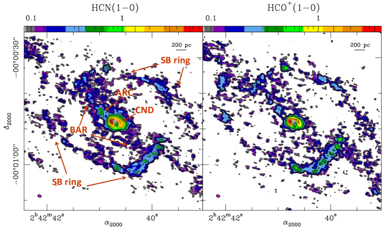
Figure 1: Left panel: velocity-integrated intensity map of HCN(1–0) of NGC 1068 obtained with ALMA. The map is shown in a logarithmic colour scale with contour levels: 3$\sigma$, 5$\sigma$, 7$\sigma$, 12$\sigma$, 24$\sigma$, 50$\sigma$, 120$\sigma$ and 200$\sigma$, where 1$\sigma$ = 0.028 Jy beam^-1km s^-1. We highlight the location of several representative regions of the emission, namely the CND, the bar, and the SB ring. Right panel: same as left panel but for the HCO⁺(1–0) line map, with the same list of contour levels but here truncated at 120$\sigma$. The position of the AGN is identified by the dark grey star marker. The black bar in the top right corner of each panel shows the spatial scale in pc. The (magenta) filled ellipses at the bottom left corners of the panels represent the ALMA beam size (1$\arcsec$.0 $\times$ 0$\arcsec$.6 at PA=69$\degr$).

3.1 Molecular gas masses

To derive the distribution of ”local” dense molecular gas mass (M_dense) from the HCN(1–0) velocity-integrated luminosities ($L_{\rm dense}^{\prime}$) we assumed the standard conversion factor commonly applied for ”global” scales, $\alpha_{\rm HCN}=10\leavevmode\nobreak\ M_{\odot}$ (K km s^-1pc²)^-1 for HCN, following Gao & Solomon (2004a), for the different ”local” scales used in this work. This factor includes a correction for Helium. A canonical ”constant” conversion factor is usually adopted in the literature for both lines, which are considered as reliable tracers of the dense molecular gas phase above densities n$\approx$10⁴cm^-3 (see, however, García-Burillo et al., 2012; Evans et al., 2020).

This fixed conversion factor assumes that the HCN(1-0) emission is originated from gravitationally-bound ”cores” or clumps with volume-averaged density n(H₂) $\sim$ 3 $\times$ 10⁴ cm^-3 and a brightness temperature T_b $\sim$ 35 K. However, under the hypothesis that the emission of the HCN line is mostly optically thick, if the volume-averaged density of the emitting clumps is lower than 3 $\times$ 10⁴ cm^-3 or if the T_b is larger than 35 K, the $\alpha_{\rm HCN}$ could be smaller than the factor suggested by Gao & Solomon (2004b). In this context, Wu et al. (2005) estimated the value of $\alpha_{\rm HCN}$ in Galactic star-forming cores, finding a slightly lower conversion factor at smaller scales: $\alpha_{\rm HCN}$= 7 $\pm$ 2 $M_{\odot}$ (K km s^-1pc²)^-1. This value differs only by 30$\%$ from the ”global” conversion factor used by Gao & Solomon (2004b), which is the one adopted in this work. We nevertheless note that adopting a lower value of the conversion factor for HCN would result in slightly lower molecular gas surface density values, particularly in the regions of the SB ring that show comparatively higher SF activity and SFE values (see discussion in Sect. 6).

We therefore derived M_dense as:

$$M_{\rm dense}[M_{\odot}]=\alpha_{\rm HCN}L_{\rm dense}^{\prime}[{\rm K\leavevmode\nobreak\ kms^{-1}pc^{2}}].$$ (5)

The line luminosity L’ is defined following Solomon et al. (1997) as:

$$L^{\prime}_{\rm dense}[{\rm K\leavevmode\nobreak\ kms^{-1}pc^{2}}]=3.25\times 10^{7}\times S_{\rm dense}\Delta V\nu_{\rm obs}^{-2}D_{L}^{2}(1+z)^{-3},$$ (6)

where the velocity-integrated fluxes $S_{\rm dense}\Delta\leavevmode\nobreak\ V$ are in Jy km s^-1 particularized for each line, the observed frequency $\nu_{\rm obs}$ is in GHz and the luminosity distance $D_{L}$ is in Mpc units.

We obtained face-on values of the dense molecular gas surface densities ($\Sigma_{\rm dense}$ in $M_{\odot}$ pc^-2 units) from:

$$\Sigma_{\rm dense}=\frac{M_{\rm dense}}{A_{\rm aperture}}\times cos(i),$$ (7)

where $i=40\degr$ is the inclination of the disk of NGC 1068 (Bland-Hawthorn et al., 1997; Brinks et al., 1997; García-Burillo et al., 2014) and $A_{\rm aperture}$ is the area of the aperture used in pc².

Similarly, we transformed the measured CO(1-0) luminosities into molecular gas masses and surface densities using the conversion prescription of Bolatto et al. (2013), which assumes a standard Galactic conversion factor $\alpha_{\rm CO}=4.4\leavevmode\nobreak\ M_{\odot}$ (K km s^-1pc²)^-1 , which already includes a correction for Helium.

We used the GILDAS task gauss-smooth to convolve the initial resolution versions of the molecular line data cubes with the appropriate Gaussian kernels adapted to generate all the image versions for the common set of spatial resolutions used in this work, which range from $\sim 40-56$ pc ($\sim 100$ pc for CO(1–0)) up to $\sim 700$ pc (see Sect. 5.1).

3.2 Star formation rates

We adopted the prescription proposed in Kennicutt & Evans (2012) regarding the conversion factor used to calculate the local SFR map from the Pa$\alpha$ line luminosities. In particular, we assumed a Kroupa initial mass function (Kroupa, 2001) as well as an intrinsic ratio for H$\alpha$/Pa$\alpha$ $\sim 7.81$ (Hummer & Storey, 1987), which applies for the case B recombination at $T_{e}$= 5000 K and $n_{e}$= 10³cm^-3. These conditions are found in starbursting galaxies (Roy et al., 2008; Rieke et al., 2009).

We obtain the SFR from the expression:

$${\rm SFR}(M_{\odot}{\rm yr^{-1}})=4.15\times 10^{-41}L({\rm Pa}\alpha,{\rm erg\leavevmode\nobreak\ s}^{-1})$$ (8)

We derived the corresponding SFR surface densities ($\Sigma_{\rm SFR}$) in units of M_⊙ yr^-1pc^-2 from:

$$\Sigma_{\rm SFR}=\frac{\rm SFR}{A_{\rm aperture}}\times cos(i),$$ (9)

We estimated the SFR for the range of spatial resolutions analysed in this work following the same procedure described in Sect. 3.1, which uses the GILDAS task gauss_smooth to convolve the initial resolution images with the appropriate Gaussian kernels.

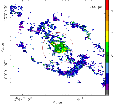
Figure 2: HCN(1–0)/HCO⁺(1–0) brightness temperature ratio map ($R_{\rm dense}$) derived at the common spatial resolution of $\simeq$56 pc. The brown circle of 8$\arcsec$-radius ($\simeq$ 560 pc) locates the inner region of the galaxy disk where the molecular outflow signature has been identified in the kinematics of molecular gas (García-Burillo et al., 2014, 2019). This region, purposely excluded from our analysis of SF relations, shows significantly higher line ratios ($R_{\rm dense}\simeq$ 1.5-3.5) compared to the SB ring ($R_{\rm dense}\simeq$0.5-1.5). Other symbols as in Fig. 1.

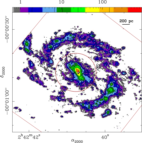
Figure 3: HST/NICMOS continuum-subtracted Pa$\alpha$ image of NGC 1068. The map is shown in colour scale with contour levels: 3$\sigma$, 9$\sigma$, 15$\sigma$, 32$\sigma$, 50$\sigma$, 120$\sigma$ and 700$\sigma$, where 1$\sigma$=0.212 10^-16erg s^-1cm^-2pixel^-1. The colour scale range is shown in units of 10^-16 erg s^-1 cm^-2 pixel^-1. The (truncated) square region identifies the outer edge of the HST/NICMOS field-of-view. The angular resolution of the image is 0$\aas@@fstack{\prime\prime}$26 $\times$ 0$\aas@@fstack{\prime\prime}$26. Other symbols as in Fig. 2.

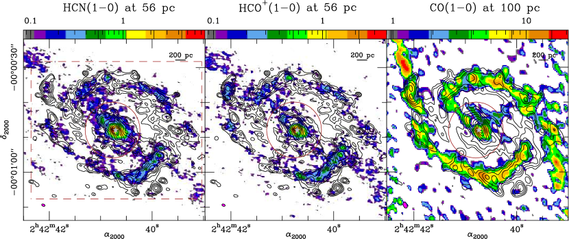
Figure 4: Left panel: overlay of the HST/NICMOS Pa$\alpha$ image (contours) on the ALMA HCN(1–0) map (colour scale). Contours with a logarithmic spacing from 3$\sigma$ to 1536$\sigma$, in steps of 0.3 dex, where 1$\sigma$=0.180^-16erg s^-1cm^-2pixel^-1. Colour scale is shown in units of Jy beam^-1km s^-1. Middle panel: same as left panel but showing the overlay of the HST/NICMOS Pa$\alpha$ contours on the ALMA HCO⁺(1–0) map (colour scale). Right panel: same as left panel but showing the overlay of the HST/NICMOS Pa$\alpha$ contours on the PdBI CO(1–0) map of Schinnerer et al. (2000) (colour scale). Contour spacing same as in left and right panels, but with 1$\sigma$=0.162 10^-16erg s^-1cm^-2pixel^-1. The (magenta) filled ellipses at the bottom left corners in all panels represent the beam sizes of the molecular line maps: 1$\arcsec$.0 $\times$ 0$\arcsec$.6 at PA=69$\degr$ (left and middle panels) and 1$\arcsec$.84 $\times$ 1$\arcsec$.09 at P.A. = 24$\degr$ (right panel). The HST/NICMOS Pa$\alpha$ images in each panel have been degraded to the corresponding spatial resolutions of the molecular gas tracers used in this comparison. Other symbols as in Fig. 2.

4 Dense molecular gas and SF maps

4.1 The HCN and HCO⁺ maps

Figure 1 shows the HCN(1–0) and HCO⁺(1–0) velocity-integrated intensity maps of NGC 1068 obtained by ALMA in the central $r\sim 2.5$ kpc of the disk. Overall, the distribution of dense molecular gas is similar to that shown by other molecular gas tracers as seen in previous interferometer images of the galaxy (Schinnerer et al., 2000; Krips et al., 2011; Tsai et al., 2012; García-Burillo et al., 2014; Viti et al., 2014; García-Burillo et al., 2019; Scourfield et al., 2020). In particular, the bulk of the HCN(1–0) and HCO⁺(1–0) emission stems from three main regions:

1. The CND. Described as an asymmetric elliptical ring of $6\arcsec\times 4\arcsec$–size ($r\sim 200$ pc), the CND shows two emission knots located $\sim 1\arcsec$ east and $\sim 1.5\arcsec$ west of the AGN. The CND ring is off-centred relative to the AGN locus. The two emission knots are bridged by weaker emission north and south of the AGN. The morphology of the HCN and HCO⁺ maps of the CND is to a large extent similar to that of the ALMA CO and CS maps (García-Burillo et al., 2014, 2019; Scourfield et al., 2020).

2. The bar. There is HCN and HCO⁺ emission in the region occupied by the $\sim 2.6$ kpc-diameter stellar bar, which is oriented along PA$=46^{\circ}\pm 2^{\circ}$ (Scoville et al., 1988; Schinnerer et al., 2000). As shown by other molecular gas tracers, the emission in this region from both lines (especially for HCN), tends to accumulate along the leading edges of the bar. We also detect significant emission in the ”bow-shock arc” feature identified in the CO(3–2) and continuum dust emission maps of García-Burillo et al. (2014) on the northeast side of the disk at $r\sim 4\arcsec-7\arcsec$ (300 pc–500 pc).

3. The SB ring. Most of the dense molecular gas in the disk concentrates in a ring of $r\sim 18\arcsec$(1.3 kpc) formed by two tightly wound spiral arms, which unfold over $\sim 180^{\circ}$ in azimuth in the disk from the ends of the stellar bar. The SB ring concentrates also most of the massive star forming complexes in the disk identified in the Pa$\alpha$ image (see Sect 4.2). The emission of HCN and HCO⁺ is unevenly distributed azimuthally over the SB ring: in both lines the emission is strongest around two regions, located at $r\sim 18\arcsec$ and PA $\sim 15^{\circ}-75^{\circ}(\pm 180^{\circ}$), where the ring is connected to the stellar bar ends. The emission of HCN and HCO⁺ in the SB ring is clumpy and it appears to be organized as coming from molecular cloud associations of $\geq 50$ pc-size. The SB ring is connected at larger radii to two emission lanes located at the edge of the HCN and HCO⁺ maps shown in Fig 1 along PA$\sim 50^{\circ}\pm 180^{\circ}$.

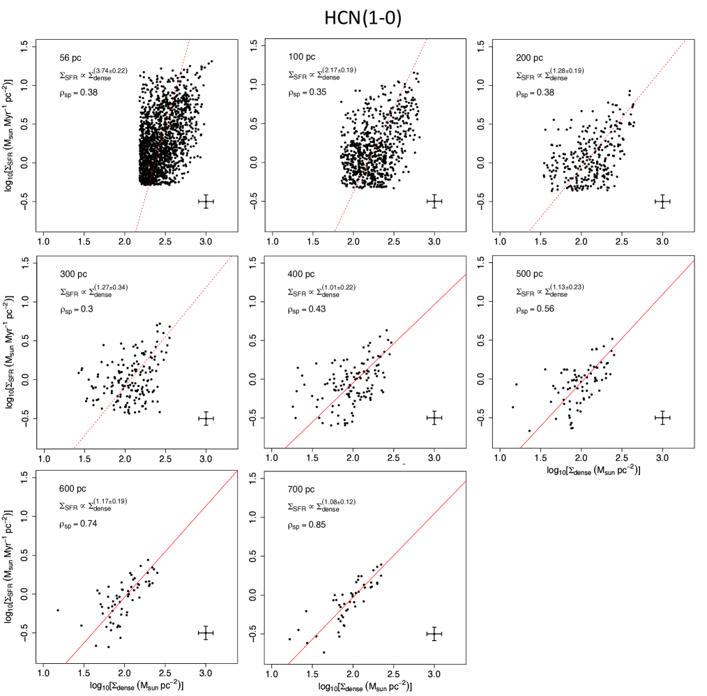
Figure 5: SFR surface density ($\Sigma_{\rm SFR}$) as a function of the dense molecular gas surface density ($\Sigma_{\rm dense}$) derived from HCN(1–0) for the different resolutions explored in this work: 56 pc, 100 pc, 200 pc, 300 pc, 400 pc, 500 pc, 600 pc and 700 pc. The red lines show the orthogonal distance regression (ODR) fits to the data. The dashed lines identify specifically the correlations that are not found to be statistically significant. We only show on both axes the data points above 3$\sigma$ which are considered in the fits. We indicate the Spearman’s rank correlation coefficients ($\rho_{\rm sp}$) and the power-law indexes ($N$) of the best fits. Vertical and horizontal errorbars at the lower right corner of each panel account for the typical uncertainties, which amount to $\pm 0.09$ dex on both axes.

Figure 2 shows the HCN-to-HCO⁺ line brightness ratio ($R_{\rm dense}$) in the disk of the galaxy. The $R_{\rm dense}$ map was obtained assuming a common 3$\sigma$ threshold on the integrated intensities of both lines. The $R_{\rm dense}$ ratio changes significantly across the different regions of the disk identified above. In particular, $R_{\rm dense}\simeq 1.5-3.5$ in the CND and the bow-shock arc region, for which we estimated a mean value $\langle R_{\rm dense}\rangle\simeq$ 2.2. On the other hand, $R_{\rm dense}\simeq 0.5-1.5$ in the SB ring and the corresponding mean value $\langle R_{\rm dense}\rangle\simeq$ 1.1.

The high $R_{\rm dense}$ values measured in the CND and the bow-shock arc are related to the molecular outflow signature identified in the kinematics of molecular gas in these regions (García-Burillo et al., 2014, 2019). The outflow is thought to be driven by the interaction of the AGN wind and the radio jet with the molecular gas in the disk in a mostly coplanar geometry. Besides leaving a distinct kinematic signature in the CND and the bow-shock arc, the outflow has left its imprint on the excitation and the chemistry of molecular gas, which is under the influence of large-scale shocks and a strong UV irradiation in these regions (Viti et al., 2014; García-Burillo et al., 2017).

4.2 The Pa$\alpha$ map

Figure 3 shows the Pa$\alpha$ image of NGC 1068 obtained at the initial resolution of the HST/NICMOS camera: $0\aas@@fstack{\prime\prime}26\times 0\aas@@fstack{\prime\prime}26$ ($\sim 18$ pc $\times 18$  pc). The central region of the image reveals strong emission stemming from an asymmetric bipolar nebula of ionized gas. Both the morphology and the kinematics of the gas in this structure have been modelled in terms of an AGN-driven wind (e.g., Crenshaw & Kraemer, 2000; Cecil et al., 2002; Das et al., 2006; Müller-Sánchez et al., 2011; Barbosa et al., 2014; Miyauchi & Kishimoto, 2020). The AGN wind occupies a hollow bicone which extends up to a radius $r\sim 8\arcsec$ (550 pc) on its northern side. The bicone feature is oriented along PA $\sim 30^{\circ}$, and is characterised by a wide opening angle ($\sim 80^{\circ}$). In our subsequent analysis of the SF relations we will therefore screen the central $r\leq 8\arcsec$ region of the galaxy, where Pa$\alpha$ cannot be considered as a reliable tracer of SF.

Outside the bright AGN bicone structure, most of the Pa$\alpha$ emission comes from the SB ring. Similar to the distribution of the dense molecular gas, SF traced by Pa$\alpha$ is not uniformly distributed throughout the SB ring. As for HCN and HCO⁺, the brightest SF complexes are located at the northeast section, and most particularly, at the southwest section of the SB ring (at PA $\sim 195^{\circ}-255^{\circ}$). In either case these are the two regions where the ring is connected to the ends of the stellar bar. Rico-Villas et al. (2021) studied the 147 GHz free-free emission associated with SF and identified a similar concentration of massive super star clusters in the bar-ring interface region.

Figure 4 shows the overlay of the HST/NICMOS Pa$\alpha$ emission image on the HCN(1–0), HCO⁺(1–0), and CO(1–0) maps. For a proper comparison we degraded the Pa$\alpha$ image to the common spatial resolution of HCN and HCO⁺ ($\sim 56$ pc), and to that of CO ($\sim 100$ pc). A visual inspection of this figure illustrates that the Pa$\alpha$ maxima do not always coincide with the strongest emission peaks in HCN, HCO⁺ or CO throughout the SB ring.

5 Star formation relations in NGC1068

5.1 Kennicutt-Schmidt laws

We use in this section the images described in Sects. 2.1 and  2.2 to obtain different versions of the pixel-wise spatially resolved KS relations in the SB ring of NGC 1068 for a set of seven spatial resolutions, ranging from $\sim 40-56$ pc ($\sim 100$ pc for CO(1–0)) up to $\sim 700$ pc. To derive $\Sigma_{\rm SFR}$ and $\Sigma_{\rm gas}$ for each spatial scale we degraded our datasets to the selected resolutions using the GILDAS task gauss-smooth. In our analysis we only considered pixels with a signal $\geq 3\sigma$ in $\Sigma_{\rm SFR}$ and $\Sigma_{\rm gas}$. Furthermore, to minimize the redundancy in the scatter plots we explored the $\Sigma_{\rm SFR}$-$\Sigma_{\rm gas}$ plane using a grid with Nyquist sampling adapted for each spatial resolution.

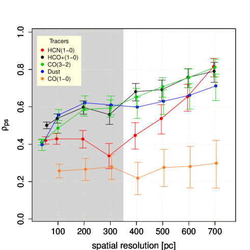
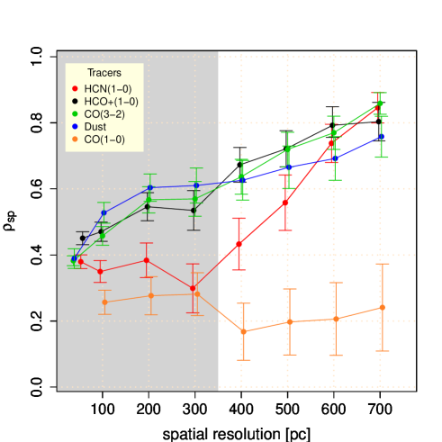
Figure 6: Pearson and Spearman correlation coefficients ($\rho_{\rm ps}$: left panel; $\rho_{\rm sp}$: right panel) of the KS laws derived for the different gas tracers used in this work as a function of the spatial resolution. Error bars represent the 67 % confidence interval around the mean values. For spatial scales larger than the range identified by the grey-coloured region ($\leq$350 pc) all the gas tracers (leaving aside CO(1–0)) show statistically significant correlations in their KS laws, defined by $p$-values $<$1$\%$ and $\rho_{\rm ps}$, $\rho_{\rm sp}>$0.4.

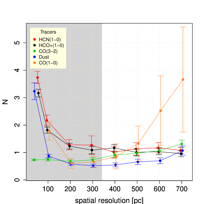
Figure 7: Power-law indexes ($N$) of the KS relations obtained from the ODR fit to the data for the different gas tracers used in this work as a function of the spatial resolution adopted. Symbols and colour codes as in Fig. 6.

Table 1: Correlation parameters obtained for the KS laws derived for different tracers and spatial scales.

	HCN(1–0)			HCO+(1–0)			CO(1–0)			CO(3–2)			Dust
scale (pc)	N	$\rho_{ps}$	$\rho_{sp}$	N	$\rho_{ps}$	$\rho_{sp}$	N	$\rho_{ps}$	$\rho_{sp}$	N	$\rho_{ps}$	$\rho_{sp}$	N	$\rho_{ps}$	$\rho_{sp}$
40	-	-	-	-	-	-	-	-	-	0.73 $\pm$0.03	0.41	0.38	3.23 $\pm$ 0.31	0.40	0.39
56	3.74 $\pm$ 0.22	0.42	0.38	3.17 $\pm$ 0.14	0.50	0.45	-	-	-	-	-	-	-	-	-
100	2.17 $\pm$ 0.19	0.43	0.35	1.82 $\pm$ 0.11	0.54	0.47	1.78 $\pm$ 0.33	0.26	0.26	0.74 $\pm$ 0.05	0.49	0.46	0.87 $\pm$ 0.07	0.56	0.53
200	1.28 $\pm$ 0.19	0.43	0.38	1.23 $\pm$ 0.11	0.60	0.55	0.61 $\pm$ 0.18	0.27	0.28	0.68 $\pm$ 0.06	0.59	0.57	0.57 $\pm$ 0.05	0.62	0.61
300	1.27 $\pm$ 0.34	0.34	0.30	1.09 $\pm$ 0.14	0.56	0.53	0.66 $\pm$ 0.21	0.28	0.28	0.73 $\pm$ 0.08	0.59	0.57	0.52 $\pm$ 0.06	0.61	0.61
400	1.01 $\pm$ 0.22	0.45	0.43	1.17 $\pm$ 0.12	0.68	0.67	0.86 $\pm$ 0.46	0.22	0.17	0.91 $\pm$ 0.11	0.65	0.69	0.55 $\pm$ 0.07	0.60	0.63
500	1.13 $\pm$ 0.23	0.54	0.56	1.01 $\pm$ 0.12	0.69	0.72	1.33 $\pm$ 0.64	0.28	0.21	0.98 $\pm$ 0.10	0.71	0.72	0.66 $\pm$ 0.11	0.63	0.67
600	1.17 $\pm$ 0.19	0.66	0.74	1.03 $\pm$ 0.11	0.76	0.79	2.16 $\pm$ 0.84	0.28	0.23	1.06 $\pm$ 0.11	0.76	0.77	0.71 $\pm$ 0.11	0.67	0.71
700	1.08 $\pm$ 0.12	0.82	0.85	0.96 $\pm$ 0.11	0.79	0.81	3.66 $\pm$ 1.92	0.30	0.24	1.31 $\pm$ 0.14	0.81	0.86	1.07 $\pm$ 0.17	0.71	0.76

Table 6 lists the power-law indexes, as well as the Pearson correlation ($\rho_{\rm ps}$) and Spearman rank ($\rho_{\rm sp}$) parameters obtained for the KS laws (in logarithmic space) for the different spatial resolutions and tracers used in this work. We carried out the fits of log($\Sigma_{\rm SFR}$) versus log($\Sigma_{\rm gas}$) using the orthogonal distance regression (ODR) method. We considered that a correlation is noteworthy and statistically significant when its two-sided p-value ¡ 1$\%$ and both $\rho_{\rm ps}$ and $\rho_{\rm sp}$ are $\geq 0.4$. Validated correlations are highlighted in boldface in Table 6. Furthermore, in order to counterbalance the dependence of the estimated $p$-values on the size of the sample, we derived these using a common number of randomly selected points for the different spatial scales.

As an illustration of the wide variance of SF relations resulting from this analysis, we show in Fig. 5 the different versions of the KS law representing $\Sigma_{\rm SFR}$ as a function of $\Sigma_{\rm dense}$ (here derived from HCN) for all the spatial scales explored in this work, namely from the ”initial resolution” (56 pc) up to 700 pc. This figure shows that the correlation becomes looser with higher resolution, and it is hardly visible in the plot with a resolution of 56 pc. The KS relation for the dense gas at the ”initial resolution” is highly scattered: $\Sigma_{\rm SFR}$ and $\Sigma_{\rm dense}$ span 1.5 dex each and show scarce evidence of correlation. We fitted a superlinear KS relation with a power-law slope $N=3.74\pm 0.22$. The correlation parameters at the ”initial resolution” have low values ($\rho_{\rm sp}=0.38$ and $\rho_{\rm ps}=0.42$) and their corresponding two-sided $p$-values $>1\%$. At scales of 100 pc we obtained a power-law slope $N=2.17\pm 0.19$ with correlation parameters of $\rho_{\rm sp}=0.35$ and $\rho_{\rm ps}=0.43$. In contrast, at 400 pc and 700 pc, the scatter in the KS relation is significantly reduced: $\Sigma_{\rm SFR}$ and $\Sigma_{\rm dense}$ span 1 dex each and the derived best-fit KS relation yields a power law index $N=1.01\pm 0.22$ and $N=1.08\pm 0.12$, with correlation parameters $\rho_{\rm sp}=0.43$, $\rho_{\rm ps}=0.45$ and $\rho_{\rm sp}$=0.85, $\rho_{\rm ps}$=0.82, with associated $p$-values $<1\%$, respectively. We represent the Kennicutt-Schmidt plots for all the tracers in Figures 28, 29, 30 and 31.

Figure 6 shows how $\rho_{\rm ps}$ and $\rho_{\rm sp}$ change as a function of the spatial resolution used for the different molecular gas and dust tracers used in this comparison. The grey-shaded region in Fig. 6 identifies the range of spatial scales where the correlation is judged not to be statistically significant. For spatial scales $\geq 300-400$ pc the correlation improves monotonically as a function of the aperture size for all gas tracers excluding CO(1–0). The $\rho_{\rm ps}$ and $\rho_{\rm sp}$ parameters for CO(1–0) show values $\leq 0.3$ for the entire range of spatial resolutions explored. We nevertheless find that for any spatial resolution the correlation parameters derived from the high density tracers (CO(3–2), HCN(1–0) and HCO⁺(1–0)) are about a factor of two to three larger than that derived from CO(1–0). Dust continuum emission shows a behaviour similar to that of the rest of high density tracers with the important particularity that the correlation is significant already at 100 pc scales. This result confirms that continuum emission is mostly sensitive to the column densities of dust which is being directly heated by recent SF activity in the SB ring.

The reported breakdown of the KS relations observed in the SB ring below a ”critical” spatial scale of $\sim 300-400$ pc is in qualitative agreement with the findings of Onodera et al. (2010), Schruba et al. (2010) in M 33 and Kreckel et al. (2018) in NGC 628. The existence of a ”critical scale” for KS laws can be explained by the diverse evolutionary states of the GMC population, which can be singled out in high spatial resolution observations. The exact value of this ”critical scale” may change from galaxy to galaxy. It may also depend on the criterion adopted to choose the data points used to generate the scatter plots: either a ”blind” pixel-wise Nyquist sampling or a ”biased” selection of apertures centred either around SF or gas emission peaks (e.g., see discussion in Williams et al., 2018). Different GMC states can reflect an ordered time sequence of star formation determined by the large-scale dynamics in galaxy disks or a more stochastic pattern due to the local dispersal of molecular gas by stellar feedback.

Figure 7 shows how the power-law index $N$ obtained from the fit to the KS relation changes as a function of the spatial resolution for the different molecular gas and dust tracers. As in Fig. 6, the grey-shaded region in Fig. 7 identifies the range of spatial scales where the correlation is not statistically significant. Overall, we find a strong scale dependence of $N$. The power-law index for HCN and HCO⁺ shows a fairly systematic decrease with the spatial resolution from $N=3.5\pm 0.3$ (at the ”initial resolution”) to $N=1.0\pm 0.1$ (at 700 pc). The value of $N$ stays around $\sim 1.0\pm 0.1$ for the whole range of spatial scales where the correlation is significant ($\geq 300-400$ pc). For CO(3–2) $N$ shows values marginally below unity in the 300 pc-500 pc range. Similarly, The value of $N$ for the dust continuum indicates a sublinear relation ($N<1$) within the range 100 pc–600 pc. The power-law becomes nevertheless linear at 700 pc as for most of the high density tracers. The reported slightly different behaviour of CO(3–2) and dust continuum relative to HCN or HCO⁺ can be attributed to the fact that, although all these tracers are sensitive to the presence of dense molecular gas, CO(3–2) and dust continuum are also to a large extent mostly sensitive to the presence of comparatively hotter molecular gas, characterised by high kinetic temperatures .

The linear behaviour of the power-law observed for all the dense gas tracers in NGC 1068 is in agreement with the results obtained in other galaxies (e.g., Gao & Solomon, 2004a, b; Graciá-Carpio et al., 2008; Wu et al., 2010; García-Burillo et al., 2012; Usero et al., 2015; Liu et al., 2015; Chen et al., 2017; Williams et al., 2018; Querejeta et al., 2019). The weak correlation found between Pa$\alpha$ and CO(1-0) at all scales indicates that the distribution of the general molecular gas traced by CO(1–0) is not strongly correlated with the current location of recent star formation in the SB ring. While we do not expect to have missed a high fraction of the CO(1–0) flux in the PdBI map on scales $\leq 200-300$ pc (see Sect. 2.1.2 and Appendix A), the likely increasing fraction of flux filtered on scales close to the $\sim 1$ kpc limit could be an explanation for the poor correlation shown by CO(1–0) in Fig. 6.

Table 2: Published work on SF relations

Reference	Galaxies	SFR tracer	Resolution (kpc)
Garcia-Burillo+12	SFG & (U)LIRG	FIR	1.7-3.6
Murphy+15	NGC 3627	33 GHz	0.3
Usero+15	galaxy disks	TIR	0.5-3.3
Bigiel+16	M51	TIR	1.1
Chen+17	M51	TIR	0.2
Viaene+18	M31	UV + 24 $\mu$m	0.1
Querejeta+19	M51	33 GHz	0.1

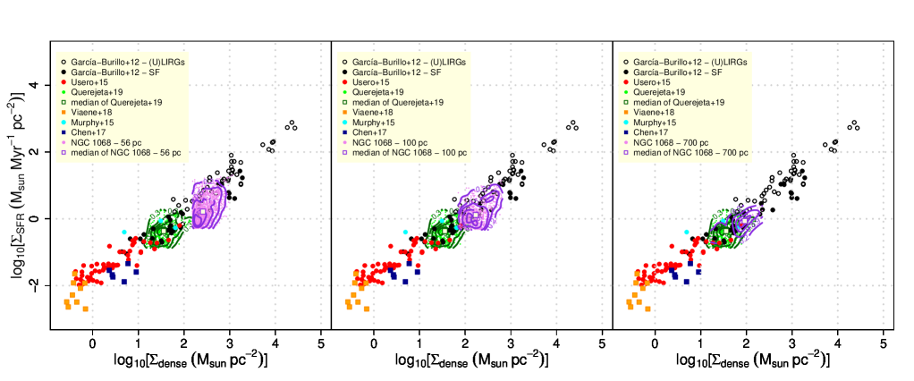
Figure 8: Comparison of the KS laws derived from HCN(1–0) in NGC 1068 with those obtained in different populations of galaxies for a range of spatial scales: global ($\simeq$a few kpc) measurements of the disks of SF galaxies and (U)LIRGs (García-Burillo et al., 2012), $\simeq$0.3-1 kpc-scale regions of the disks of nearby SF galaxies (Murphy et al., 2015; Usero et al., 2015; Bigiel et al., 2016), and 0.1-0.2 kpc-size regions in the disk of M 51(Chen et al., 2017; Viaene et al., 2018; Querejeta et al., 2019). For the sake of a better comparison with the reference sample, the scatter-plots for NGC 1068 (magenta circles and isodensity contours) are displayed for three spatial resolutions: 56 pc (left panel), 100 pc (middle panel), and 700 pc (right panel). The scatter-plot for M 51 at 100 pc resolution is displayed by the green cricles and isodensity contours. The open squares stand for the median values of the distributions in NGC 1068 and M 51.

5.2 The Kennicutt-Schmidt laws of NGC 1068 in context

We compare in this section the KS relations derived from HCN(1–0) in the SB ring of NGC 1068 with those obtained by previous works in different populations of galaxies. Table 8 lists the references used in this comparison. These works comprise galaxy-scale studies of SF galaxies (SFG) and (U)LIRG (e.g., see compilation by García-Burillo et al., 2012, and references therein), as well as spatially resolved studies of individual galaxies (Usero et al., 2015; Murphy et al., 2015; Bigiel et al., 2016; Chen et al., 2017; Viaene et al., 2018; Querejeta et al., 2019). These references use the equations of Section 3 to convert HCN(1–0) intensities into (deprojected) surface densities of dense gas and adopt the same HCN conversion factor used in this paper. However, the SF tracers chosen in these works are different, as detailed in Table 8.

Figure 8 compares the different versions of the KS law derived from HCN(1–0) in NGC 1068 at three spatial resolutions (56 pc, 100 pc, and 700 pc) with those obtained in the references listed in Table 8. NGC 1068 data lie within the linear power-law branch occupied by the rest of the galaxies shown in Fig. 8. Galactic dense cores, at sub-pc scale, align along the same relationship (Wu et al., 2005, 2010; Rosolowsky et al., 2011; Stephens et al., 2016; Shimajiri et al., 2017). Taken at face value, this suggests that the star formation efficiency (SFR per unit dense molecular mass) is nearly constant on average. As expected, the internal scatter in the distribution NGC1068 data points is lower as we move to larger apertures. Furthermore, NGC 1068 data points shift toward lower surface densities within the power-law as we move to larger apertures.

Compared at a common scale of 100 pc, the SB ring of NGC 1068 appears as a more extreme environment relative to the SF regions of M51 studied by Querejeta et al. (2019). As illustrated in Fig. 8, the median values of the distributions of $\Sigma_{\rm SFR}$ and $\Sigma_{\rm dense}$ are about a factor of three to five higher in NGC 1068: $\Sigma_{\rm SFR}$[NGC1068] $\simeq 1.5\leavevmode\nobreak\ M_{\sun}$ Myr^-1pc${}^{-2}\simeq 3\times\Sigma_{\rm SFR}$[M51] and $\Sigma_{\rm dense}$[NGC1068] $\simeq 174\leavevmode\nobreak\ M_{\sun}$ pc${}^{-2}\simeq 5\times\Sigma_{\rm dense}$[M51]. Furthermore, when examined at scales of 700 pc, NGC 1068 occupies in the KS plot a position intermediate between that of normal galaxies and (U)LIRGs, a result that hints at the relatively extreme conditions in the SB ring.

5.3 Environmental dependence of the star formation efficiency of the dense gas

The observed linear relation between $\Sigma_{\rm SFR}$ and $\Sigma_{\rm dense}$ shown in Fig. 8 has been considered as evidence of the validity of density-threshold models of SF. For these models the SF efficiency of dense molecular gas, defined as SFE_dense=$\Sigma_{\rm SFR}$/$\Sigma_{\rm dense}$ or its inverse, which represents the depletion time of the dense gas ($T_{\rm dep}^{\rm dense}$=SFE${}_{\rm dense}^{-1}$), are about constant in different populations of galaxies and also for different dynamical environments within galaxies (Gao & Solomon, 2004b; Wu et al., 2005; Lada et al., 2010, 2012; Evans et al., 2014). In this section we use the NGC 1068 data to explore the existence of an environmental dependence of SFE_dense inside the SB ring.

Figure 9 (left panel) overlays the HST/NICMOS Pa$\alpha$ image on the HCN(1–0) map of NGC 1068 obtained at the ”initial resolution” of 56 pc. We identify the positions used to extract the fluxes of Pa$\alpha$ and HCN(1–0) over the SB ring from the Nyquist-sampled grid . SFE_dense values span almost 1.5 dex and show a highly scattered distribution as a function of $L^{\prime}_{\rm HCN}$ around an ”apparently” constant mean value of about 0.01 Myr^-1, equivalent to a $T_{\rm dep}^{\rm dense}\sim 100$ Myr (see right panel of Fig. 9). This result is similar to the findings of Gallagher et al. (2018) and Querejeta et al. (2019) obtained from their high spatial resolution images of a sample of galaxies. Notwithstanding that we might attribute part of the scatter in the SFE_dense–$L^{\prime}_{\rm HCN}$ plot to possible small-scale variations of the $\alpha_{\rm HCN}$ conversion factor, any plausible range for these potential variations would nevertheless fall short of accounting for the bulk of the 1.5 dex span shown in Fig. 9.

Although Figs. 8 and  9 indicate that there is an overall relationship between the HCN luminosity and recent star formation in the SB ring, we explore below the existence of systematic trends in SFE _dense. With this aim, we selected within our initial grid a number of non-overlapping 56 pc-size apertures centred on local maxima either in the HCN or the Pa$\alpha$ maps, following the same procedure used by Querejeta et al. (2019) in their analysis of M 51 data. The local maxima were identified as the pixels with peak intensities within circular regions (”clumps”), obtained from successive cuts in the maps. We therefore started from a high threshold (a large multiple of the noise level) and iteratively explored lower values from isolated circular regions. To collect a similar number of points selected from HCN and Pa$\alpha$ peaks we continued to identify new clumps down to different threshold values of 12$\sigma$ and 44$\sigma$, respectively. We use different colours to identify in the two panels of Fig. 9 the apertures centred on HCN peaks (blue colour), on Pa$\alpha$ peaks (red colour), and also on the $10\%$ of the apertures showing the highest values of SFE_dense (green colour).

Figure 9 shows that the apertures showing the top $10\%$ SFE_dense values are not uniformly distributed throughout the SB ring. High SFE_dense values are preferentially located at the southwest and northeast sections of the ring where the latter is connected to the ends of the stellar bar. We also identify high SFE_dense values further out at the northeast extreme of the SB ring. As expected, the clumps with the strongest Pa$\alpha$ emission are also located in the regions with the highest SFE_dense. Furthermore, although the overall distribution of the highest (dense) gas column density apertures also corresponds to the ends of the stellar bar, on small-scales there is no one-to-one correspondence between Pa$\alpha$ and the HCN peaks. This reflects the significant variance in the evolutionary states of the dense gas clumps in these regions. In particular, the gas ridge traced by HCN maxima tend to appear ”upstream” relative to the Pa$\alpha$ maxima at the southwest section of the SB ring .

In order to minimize the bias introduced due to the presence of HCN in the two axes of the right panel of Fig. 9, we replaced HCN by HCO⁺ luminosities along the x-axis by selecting from our grid of points those positions satisfying $L^{\prime}_{\rm HCO^{+}}>3\sigma$. Figure 10 shows the results obtained following the same steps leading to Fig. 9. As expected, Fig. 10 eliminates the slight anti-correlation trend identified in the SFE_dense-$L^{\prime}_{\rm HCN}$ plot of Fig. 9, but the main results described above remain virtually unchanged.

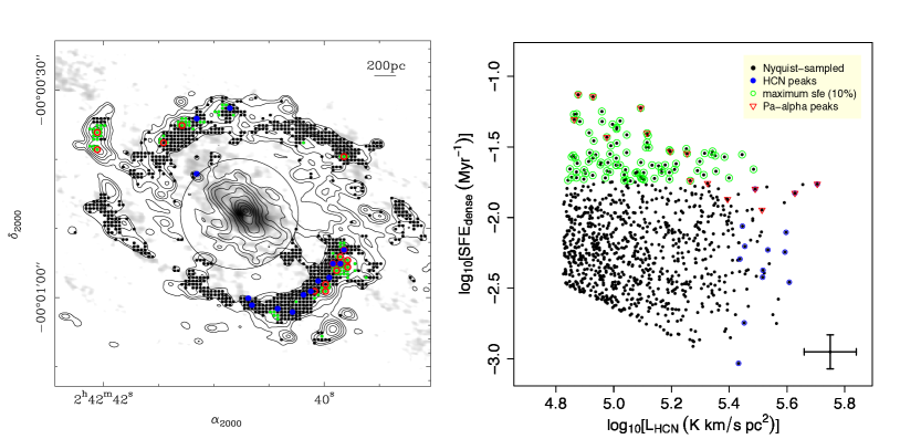
Figure 9: Left panel: overlay of the HST/NICMOS Pa$\alpha$ image (contours) on the HCN(1–0) map (grey scale). Contours and grey scale as in Fig. 4. The set of 56 pc-size circular apertures used to extract the fluxes of Pa$\alpha$ and HCN(1–0) are colour-coded differently, depending on whether they are centred on HCN peaks (in blue colour), on Pa$\alpha$ peaks (in red colour), or on the $10\%$ of the apertures showing the highest values of SFE_dense (in green colour). The black dots identify the centres of all the Nyquist-sampled 56 pc-size apertures where there are reliable estimates of SFE_dense across the SB ring. Right panel: distribution of SFE_dense values (in Myr^-1-units) as a function of L_HCN (in K km^-1pc²-units) in the SB ring of NGC 1068. Symbols as in left panel. Vertical and horizontal errorbars at the lower right corner of the panel account for the typical uncertainties, which amount to $\pm 0.13$ dex and $\pm 0.09$ dex, respectively.

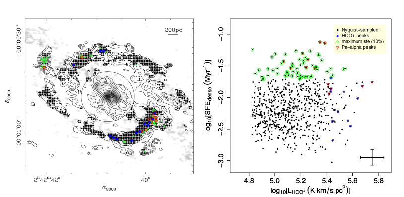
Figure 10: Same as Fig. 9 but replacing HCN(1–0) by HCO⁺(1–0) along the x-axis of the right panel.

6 Star formation efficiency and dense gas fraction

The overall SF efficiency of molecular gas (SFE_mol) can be expressed as the product of SFE_dense and the dense gas fraction ($F_{\rm dense}$), namely: SFE${}_{\rm mol}\equiv$ SFE${}_{\rm dense}\times F_{\rm dense}$. There is mounting evidence supporting the existence of significant variations in SFE_dense and $F_{\rm dense}$ as a function of the galactic environment, based on observations of molecular clouds in the centre of our Galaxy (Longmore et al., 2013; Kruijssen et al., 2014) and in nearby galaxies for a range of spatial scales (Usero et al., 2015; Bigiel et al., 2015, 2016; Gallagher et al., 2018; Querejeta et al., 2019; Jiménez-Donaire et al., 2019; Bešlić et al., 2021). In the following sections we study the trends in SFE_dense and $F_{\rm dense}$ as a function of a number of physical variables with the aim of resolving the degeneracy of SF laws in the SB ring of NGC 1068. Table 11 lists the Spearman rank parameters for the different combinations of variables and spatial scales explored below.

Table 3: Spearman rank parameters for different scaling relations.

	SFEdense vs. $\Sigma_{\rm star}$	Fdense vs. $\Sigma_{\rm star}$	SFEdense vs. $\sigma_{\rm HCN}$	Fdense vs. $\sigma_{\rm HCN}$	$\Sigma_{\rm SFR}$ vs. Fdense	Tdep vs. bHCN	SFEdense vs. Fdense
56 pc	0.10	–	-0.22	–	–	-0.19	–
100 pc	0.15	0.40	-0.28	0.10	0.22	-0.43	0.03
400 pc	0.59	0.67	-0.06	0.50	0.62	-0.66	0.34

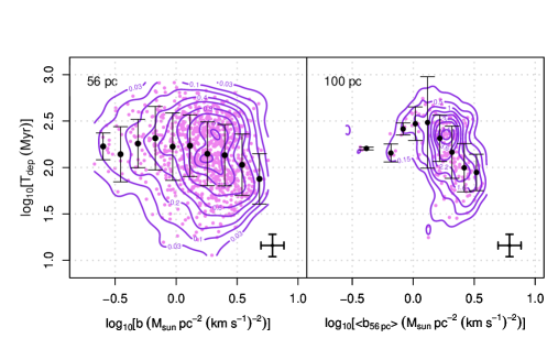
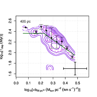
Figure 11: Depletion time of the dense molecular gas estimated from HCN, $T_{\rm dep}^{\rm dense}$ $\equiv$ $\Sigma_{\rm dense}$/$\Sigma_{\rm SFR}$, as a function of the self-gravity of the gas, measured by the parameter b $\equiv$ $\Sigma_{\rm dense}$/$\sigma^{2}$, at different spatial scales (magenta circles and isodensity contours): 56 pc, namely the ”initial resolution” of ALMA observations (left panel), 100 pc (middle panel), and 400 pc (right panel). A significant trend in $T_{\rm dep}^{\rm dense}$ as a function of $b$, identified in the middle and right panels, indicates a higher rate of star formation per unit mass of dense gas for regions with stronger self-gravity. Values of $\langle b\rangle$ for the 100 pc and 400 pc apertures were derived from an intensity–weighted average of $b$ evaluated at the Nyquist- sampled grid of points for each aperture. Values of $T_{\rm dep}^{\rm dense}$ were derived using a Gaussian-weighted average. Black circles show median $T_{\rm dep}^{\rm dense}$, and errorbars indicate the rms scatter in the bins. The green lines at the right panel identify the two regimes in the $T_{\rm dep}^{\rm dense}$-$\langle b\rangle$ plot found by the MARS algorithm to fit the data using 400 pc as averaging scale. Vertical and horizontal errorbars at the lower right corner of each panel account for the typical uncertainties, which amount to $\pm 0.13$ dex and $\pm 0.09$ dex, respectively.

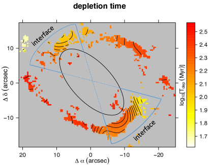
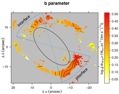
Figure 12: Left panel: map of the depletion time of the dense molecular gas ( $T_{\rm dep}^{\rm dense}$) obtained after using 400 pc as averaging scale. Contour levels for log₁₀( $T_{\rm dep}^{\rm dense}$) go from 1.50 to 2.22 in steps of 0.045 (in Myr). Right panel: map of the intensity-weighted average of the $b$ parameter ($\langle b\rangle$) in the SB ring of NGC 1068 obtained after using 400 pc as averaging scale. Contour levels for log₁₀($\langle b\rangle$) go from 0.075 to 0.45 in steps of 0.025 (in $M_{\sun}$ pc^-2 (km s^-1)^-2). $\Delta\alpha$ and $\Delta\delta$ offsets in arc seconds are relative to the phase tracking centre of ALMA. The ellipse identifies the extent of the nuclear stellar bar in the disk. We highlight the approximate extent of the bar-ring interface region in both panels.

6.1 Trends as a function of the boundedness of the gas

In this section we use an alternative prescription for the SF relations of the SB ring, which includes explicitly the dependence of SFE_dense on a combination of $\Sigma_{\rm dense}$ and the gas velocity dispersion ($\sigma$), in an attempt to resolve the degeneracy associated with the scatter in the SFE_dense-$L^{\prime}$(HCN) plot of Fig. 9. This approach was first used by Leroy et al. (2017) in their analysis of SF relations in M 51 and also adopted by Kreckel et al. (2018) in a similar study carried out in NGC 628. Leroy et al. (2017) and Kreckel et al. (2018) used CO(1–0) and CO(2–1) to trace the bulk of the molecular gas on 40-50 pc-scales in M 51 and NGC 628, respectively. In the following analysis we use HCN(1–0) to specifically trace the dense molecular gas in the SB ring of NGC 1068 on spatial scales ($\sim 56$ pc) comparable to those explored by Leroy et al. (2017) and Kreckel et al. (2018) .

The degree of self-gravity or boundedness of molecular gas clouds determines to a large extent their ability at forming stars. The virial parameter, defined as $\alpha_{\rm vir}\approx$ 2KE/UE, captures the balance of gravitational potential ($UE$) and kinetic energy ($KE$) and is commonly used in turbulent models of SF as a predictor of the efficiency of star formation (Krumholz & McKee, 2005; Padoan et al., 2012, 2017).

We define similarly to Leroy et al. (2017) the boundedness parameter, here particularized for the dense molecular gas phase traced by HCN, as $b_{\rm 56pc}\equiv\Sigma_{\rm dense}/\sigma^{2}\propto UE/KE\propto\alpha^{-1}_{\rm vir}$, where $\sigma$ is the velocity dispersion and $\Sigma_{\rm dense}$ is the column density of dense gas measured both at the ”initial resolution” of 56 pc. We derived intensity-weighted averages of $b_{\rm 56pc}$ using two different apertures $\Delta A=100$ pc and $400$ pc over the Nyquist sampled grid, defined as follows:

$$\langle b\rangle_{\rm\Delta A}(x_{0},y_{0})=\dfrac{\Sigma w(x,y)I_{\rm 56pc}(x,y)b_{\rm 56pc}(x,y)}{\Sigma w(x,y)I_{\rm 56pc}(x,y)}.$$ (10)

The Gaussian weight $w(x,y)$ is defined as:

$$w(x,y)=exp\left(\frac{-(\theta(x,y,x_{0},y_{0}))^{2}}{2\sigma^{2}_{\rm\Delta A}}\right),$$ (11)

where $\theta(x,y,x_{0},y_{0})$ is the angular distance from the measurement point $(x_{0},y_{0})$, $\sigma_{\rm\Delta A}$ is the $\sigma$-width of the Gaussian averaging beam, and $\Delta A$ corresponds to the adopted averaging scale (100 pc and 400 pc in our case). In Eq. 10, $b_{\rm 56pc}$ and $I_{\rm 56pc}$ are the boundedness parameter and the HCN integrated intensity, respectively, measured at a generic position $(x,y)$ of the grid .

Figure 11 shows how the depletion time of the dense molecular gas estimated from HCN, $T_{\rm dep}^{\rm dense}$ $\equiv$ SFE${}_{\rm dense}^{-1}$, changes as a function of the self-gravity of the gas, measured by the $b$ parameter, at three spatial scales: 56 pc (the ”initial resolution”), 100 pc, and 400 pc. The values of $\langle b\rangle_{\rm\Delta A}$ for the 100 pc and 400 pc apertures were derived from Eq. 10. Furthermore, similarly to the rest of the physical parameters analysed in Sects. 6.2 to 6.4, the average value of $T_{\rm dep}^{\rm dense}$ inside the two values of $\Delta A$ were derived using the Gaussian weighting function of Eq. 11.

Figure 11 shows a significant monotonic decrease of $T_{\rm dep}^{\rm dense}$ as function of $\langle b\rangle_{\rm\Delta A}$ when we represent these parameters averaged over the two apertures. Specifically, we obtain (anti) correlation Spearman rank parameters $\rho_{\rm sp}=-0.43$ and $-0.66$ for $\Delta A=100$ pc and $400$ pc, respectively, and associated two-sided $p$-values $<1\%$. Overall, this is indicative of a higher rate of star formation per unit mass of dense gas (lower $T_{\rm dep}^{\rm dense}$) for regions characterised by a stronger self-gravity (higher $b$ or lower $\alpha_{\rm vir}$ values).

The anti-correlation reported above is more pronounced in the intensity-weighted version of the plot derived at 400 pc scales. We identify a turnover in the $T_{\rm dep}-b$ scatter plot for $\Delta A=400$ pc located around log${}_{\rm 10}(\langle b\rangle)\simeq\leavevmode\nobreak\ 0.2\leavevmode\nobreak\ M_{\sun}$pc^-2(km s^-1)^-2, as shown in the right panel of Fig. 11. The observed change of tendency around this point defines two regimes in the $T_{\rm dep}-b$ parameter space. To quantify the two-regime trend and the turnover, we used the Multivariate Adaptive Regression Splines (MARS) fit routine from the Rstudio package. We performed the MARS fit on 100 realizations of the $T_{\rm dep}$ vs. $b$ relation at $\Delta A=400$ pc taking into account the data uncertainties. From this Monte Carlo simulation, we obtained a turnover at log${}_{\rm 10}(\langle b\rangle)=\leavevmode\nobreak\ 0.23\pm 0.02\leavevmode\nobreak\ M_{\sun}$pc^-2(km s^-1)^-2 which is indicated in the right panel of Fig. 11. Furthermore, for $\langle b\rangle$ values below the turnover the trend is approximately flat (slope = 0.02 $\pm$ 0.11). In contrast, the MARS routine fits a slope = -1.59 $\pm$ 0.15 beyond the turnover. This slope is larger than the one obtained by Leroy et al. (2017) ($\simeq-0.9$) in their analysis of the M 51 CO(1–0) data, derived using the same averaging spatial scales (400 pc). Kreckel et al. (2018) found nevertheless no significant correlation in their analysis of the CO(2–1) data of NGC 628, which used an averaging scale of 500 pc. Compared to the shallower or inexistent trends identified in M 51 and NGC 628, the steeper decline of $T_{\rm dep}^{\rm dense}$ with $\langle b\rangle$ in the SB ring of NGC 1068 reflects the tighter link between the boundedness of dense molecular gas and star formation efficiency .

Figure 12 shows the spatial distribution of $T_{\rm dep}^{\rm dense}$ and $\langle b\rangle$ derived for $\Delta A=400$ pc in the SB ring of NGC 1068. The $T_{\rm dep}^{\rm dense}$ map of Fig. 12 confirms the picture drawn from the analysis of Sect. 5.3: the regions showing comparatively higher (lower) SFE_dense ($T_{\rm dep}^{\rm dense}$) values are preferentially located closer to the region where the SB ring is connected to the ends of the stellar bar around PA $\sim 15^{\circ}-75^{\circ}(\pm 180^{\circ}$). We also see a similar spatial segregation in the $\langle b\rangle$ map, which shows higher $\langle b\rangle$ values closer to the bar-ring interface region. Besides the azimuthal dependence of $T_{\rm dep}^{\rm dense}$ and $\langle b\rangle$ within the SB ring, we also identify a radial dependence for both parameters especially in the southern section of the bar-ring interface: in particular, the highest (lowest) $T_{\rm dep}^{\rm dense}$ ($\langle b\rangle$) values tend to appear ”upstream” (smaller radii) along the gas circulation lines if we assume that the sense of rotation of the gas in the disk is counterclockwise. The two branches in the $T_{\rm dep}^{\rm dense}$-$\langle b\rangle$ plot of Fig. 11 correspond to a large extent to the two regions of the SB ring identified in Fig. 12. Similar results are found in Appendix E when we consider the HCO⁺ as dense gas tracer. The trends and statistical parameters derived are practically identical to the ones obtained using HCN.

We can speculate if the reported trends of $T_{\rm dep}^{\rm dense}$ as a function of $\langle b\rangle$ for $\Delta A=400$ pc, visualized in Figs. 11 and 12, could be entirely attributed to potential variations of the $\alpha_{\rm HCN}$ conversion factor on these spatial scales. In this context it is worth noting that the range explored by $T_{\rm dep}^{\rm dense}$ as a function of $\langle b\rangle$, which amounts to 0.6 dex ($\simeq$a factor of four), is a significant factor of three larger than the differences found between the ”global” kpc scale and the ”small” pc scale HCN conversion factors reported by Wu et al. (2005), as mentioned in Sect 3.1. Although we have no way of confirming or refuting the existence of significantly larger changes of $\alpha_{\rm HCN}$ based on our data, we note that adopting a lower value of the conversion factor for HCN would result in lower molecular gas surface densities, particularly in the regions of the SB ring of NGC1068 that happen to show comparatively higher (lower) SFE_dense ($T_{\rm dep}^{\rm dense}$) values. These regions very likely comprise a collection of hot core-like clouds akin to the Galactic SF cores studied by Wu et al. (2005) for which $\alpha_{\rm HCN}^{\rm cores}\simeq 0.7\times\alpha_{\rm HCN}^{\rm global}$. As a direct consequence, the trends shown in Figs. 11 and 12 would be further enhanced rather than being suppressed.

6.2 Trends as a function of the dense gas fraction

Observations of molecular gas in our Galaxy and in a number of nearby galaxies have found clear evidence of trends in SFE_dense as a function of $F_{\rm dense}$, which are indicative of anti-correlation (e.g., Longmore et al., 2013; Chen et al., 2015; Murphy et al., 2015; Usero et al., 2015; Bigiel et al., 2016; Gallagher et al., 2018; Querejeta et al., 2019; Jiménez-Donaire et al., 2019). In particular, Usero et al. (2015) found that SFE_dense is about 6–8 times lower near the galaxy centres than in the outer regions of the galaxy disks analysed in their IRAM-30m survey. This radial trend is reversed for $F_{\rm dense}$ in their sources. Furthermore, Longmore et al. (2013) found anomalously low SFR values in a large fraction of high-density molecular clouds in the centre of the Milky Way, suggestive of an anticorrelation between SFE_dense and $F_{\rm dense}$. A similar trend has been found recently by Querejeta et al. (2019) in their study of M 51, and by Jiménez-Donaire et al. (2019) from an analysis of the data obtained by the EMPIRE survey in nine spiral galaxies. We examine in this section the existence of a trend in SFE_dense as a function of $F_{\rm dense}$ in the SB ring of NGC 1068.

We define two proxies for the ”dense gas fraction” in the SB ring. First, the ratio of the dense molecular gas surface density derived from HCN (1–0) to the bulk molecular gas surface density derived from from CO(1–0), that is, $F_{\rm dense}$=$\Sigma_{\rm dense}$/$\Sigma_{\rm mol}$ $\propto$ $I_{\rm HCN(1-0)}$/$I\rm_{CO(1-0)}$. We consider that CO line traces the bulk of the molecular gas in the galaxy ($n$(H₂) $\gtrsim 10^{2-3}$cm^-3), while HCN traces material with $n$(H₂) $\gtrsim 10^{4-5}$cm^-3. We therefore use the HCN(1–0)/CO(1–0) line ratio (hereafter $R_{\rm HCN/CO}$) as a proxy for the dense gas fraction in the SB ring. Secondly, we also use the CO(3–2)/CO(1–0) ratio (hereafter $R_{\rm 3-2/1-0}$) in the SB ring derived by García-Burillo et al. (2014) as an alternative proxy for $F_{\rm dense}$.

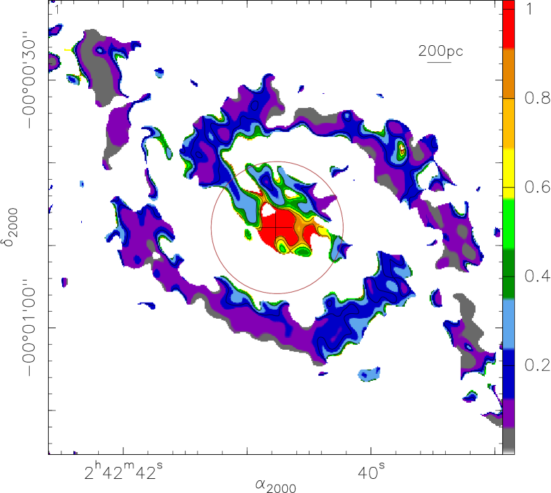
Figure 13: HCN(1–0)/CO(1–0) brightness temperature ratio map ($R_{\rm HCN/CO}$; colour scale and contours) derived at the common (lower) spatial resolution of the CO(1–0) observations of Schinnerer et al. (2000) ($\simeq$100 pc). The brown circle of 8$\arcsec$-radius ($\simeq$ 560 pc) locates the inner region excluded from our analysis of SF relations.

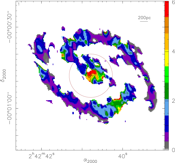
Figure 14: Same as Fig. 13 but showing the CO(3–2)/CO(1–0) brightness temperature ratio map ($R_{\rm 3-2/1-0}$; colour scale and contours) derived at the common (lower) spatial resolution of the CO(1–0) observations.

Figures 13 and 14 show $R_{\rm HCN/CO}$ and $R_{\rm 3-2/1-0}$ in $T_{\rm mb}$ units. To derive the brightness temperature ratios, we degraded the HCN(1–0) and CO(3–2) maps to the spatial resolution of the CO(1–0) observations of Schinnerer et al. (2000). The $R_{\rm HCN/CO}$ ratio changes significantly across the disk of NGC 1068. The highest values of $R_{\rm HCN/CO}$, $>0.4-1.2$, correspond to the CND. Although in the SB ring $R_{\rm HCN/CO}$ shows a wide range of values, this ratio is higher in the bar-ring interface region ($R_{\rm HCN/CO}\sim 0.2-0.4$) than elsewhere in the ring ($R_{\rm HCN/CO}\sim 0.05-0.2$). The $R_{\rm 3-2/1-0}$ ratio, shown in Fig. 14, changes also significantly across the disk. The $R_{\rm 3-2/1-0}$ ratio in the CND ($\sim 2-6$) is higher than in the SB ring, in agreement with previous estimates by Krips et al. (2011) and Tsai et al. (2012). While the average ratio is $\sim 1.2\pm 0.02$ in the SB ring , $R_{\rm 3-2/1-0}$ is higher in the bar-ring interface region ($R_{\rm 3-2/1-0}\sim 0.6-3$) and comparatively lower elsewhere in the ring ($R_{\rm 3-2/1-0}\sim 0.1-0.8$).

The $R_{\rm HCN/CO}$ ratio is hardly sensitive to kinetic temperature ($T_{\rm k}$), as the energy levels giving rise to both rotational transitions are similar ($E_{\rm k}$[$J=1$, CO] $\sim 5.5$ K, $E_{\rm k}$[$J=1$, HCN] $\sim 4.3$ K). However, as the excitation of both CO lines are sensitive to both $n$(H₂) and $T_{\rm k}$, $R_{\rm 3-2/1-0}$ is comparatively a more indirect and less straightforward tracer of $F_{\rm dense}$ relative to $R_{\rm HCN/CO}$. Leaving aside the uncertainties on the value of $\alpha_{\rm HCN}$ in SF regions, which may reflect a peculiar hot-core like chemistry, $R_{\rm HCN/CO}$ is therefore the most reliable proxy for the dense gas fraction and as such is widely used in extragalactic studies, and we therefore adopt it in the following analysis. In either case, we note that both line ratios suggest a higher excitation of HCN(1–0) and CO(3–2) lines relative to CO(1–0) in the bar-ring interface region.

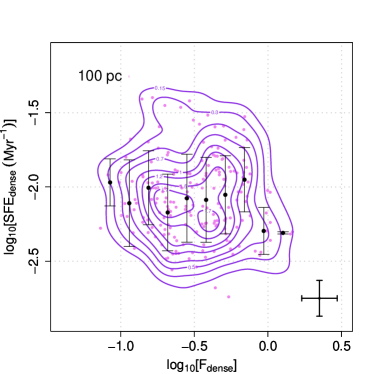
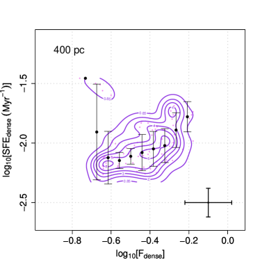
Figure 15: Star formation efficiency of the dense gas (SFE_dense) as a function of dense gas fraction ($F_{\rm dense}$: estimated from the HCN(1–0)-to-CO(1–0) line ratio of Fig. 13) in NGC 1068 using two averaging scales: 100 pc (left panel) and 400 pc (right panel). Magenta circles correspond to data measurements evaluated at the Nyquist-sampled grid of points after convolution with the appropriate Gaussian for each aperture. Black circles show median SFE_dense values and errorbars indicate the rms scatter in the bins. Vertical and horizontal errorbars at the lower right corner of both panels account for the typical uncertainties, which amount to $\pm 0.13$ dex.

Figure 15 represents SFE_dense as a function of $F_{\rm dense}$ estimated from $R_{\rm HCN/CO}$ in the SB ring. We adopted the same approach followed in Sect. 6.1 to obtain estimates of both variables over two averaging scales: $\Delta A$=100 pc and 400 pc. Figure 15 shows that there is no significant trend in SFE_dense as a function of $F_{\rm dense}$ for $\Delta A$=100 pc: we estimate a Spearman rank parameter $\rho_{\rm sp}=+0.03$ with a two-sided $p$-value $>1\%$. For $\Delta A=400$ pc there is nevertheless a more significant positive correlation ($\rho_{\rm sp}=+0.34$, with a $p$-value $<1\%$). This trend is a direct consequence of the spatial distribution of SFE${}_{\rm dense}^{-1}$ and $F_{\rm dense}$ shown, respectively, in Figs. 12 and  13. The monotonic increase shown in the right panel of Fig. 15 suggests that the comparatively denser molecular gas of the bar-ring interface region inside the SB ring forms stars at higher rate per unit dense gas mass.

This result seems to be in contradiction with the anticorrelation trends found between SFE_dense and $F_{\rm dense}$ in previous works in other galaxies. Specifically, Usero et al. (2015) found an index $N\sim-1.6$ for the SFE${}_{\rm dense}\propto F_{\rm dense}^{N}$ power-law fitting their data. A similar index ($N\sim-1.5$) can be estimated from the data compiled by Querejeta et al. (2019).

6.3 Trends as a function of the stellar mass surface density

Several works studying the existence of trends in SFE_dense as a function of $\Sigma_{\rm star}$ on kpc-scales in a number of nearby galaxies have found that SFE_dense is seen to decrease in the central parts of galaxy disks, namely in regions characterised by high $\Sigma_{\rm star}$. These observations also showed that $F_{\rm dense}$ tends to increase systematically with $\Sigma_{\rm star}$ (Chen et al., 2015; Usero et al., 2015; Bigiel et al., 2016; Gallagher et al., 2018; Jiménez-Donaire et al., 2019). Querejeta et al. (2019) studied different regions in the disk of M 51 and found that similar correlations are recovered at 100 pc-scales. We investigate below the trends in SFE_dense and $F_{\rm dense}$ as a function of $\Sigma_{\rm star}$ in the SB ring of NGC 1068.

Near-infrared emission is commonly used to trace the stellar mass in nearby galaxies, since light at these wavelengths mainly comes from old stars and is less affected by extinction (Quillen et al., 1994). With this aim, we used the HST near-infrared (NIR) continuum narrow-band image of NGC 1068 at 1.9 $\mu$m, obtained with the F190N filter on the NICMOS 3 camera, to trace the distribution of the stellar mass in the disk of the galaxy. We assumed a constant mass-to-light ratio $M/L_{1.9\mu m}=0.2M_{\odot}$/$L_{\odot}$ (e.g., see Querejeta et al., 2015) to obtain the local stellar mass surface density. Figure 16 overlays the HCN(1–0) integrated intensity contours on the HST/NICMOS F190N image. The stellar bar feature is easily identified in the NIR image. Judging from the overall distribution of $\Sigma_{\rm star}$ in the disk, it appears that the bar-ring interface is characterised by higher $\Sigma_{\rm star}$ values compared to the regions located elsewhere in the SB ring.

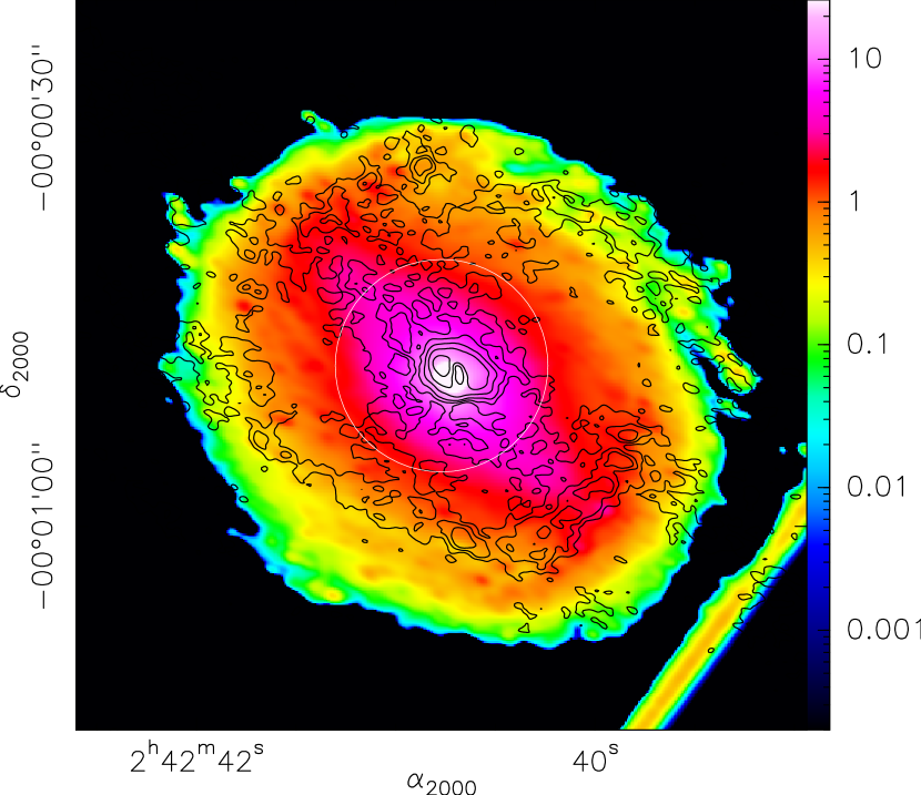
Figure 16: Overlay of the ALMA HCN(1–0) map (contours) on the HST/NICMOS F190N continuum image at 1.9 $mu$m HST (colour scale as shown in Jy). Contour spacing: 3$\sigma$, 7$\sigma$, 12$\sigma$, 24$\sigma$, 50$\sigma$ and 120$\sigma$, where 1$\sigma$=0.028 Jy beam^-1 km s^-1. The white circle of r = 8$\arcsec$ locates the inner of the galaxy, excluded of our analysis. The HST/NICMOS F190N image has been degraded to the spatial resolution of HCN(1–0) (1$\arcsec$ $\times$ 0$\arcsec$.6 $\approx$ 50 pc).

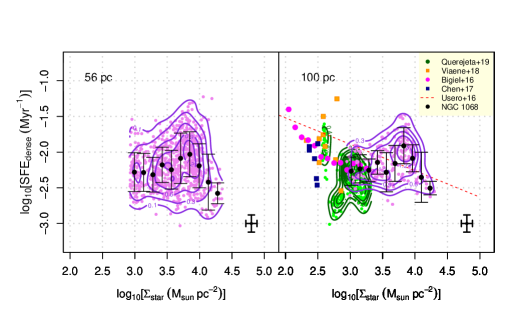
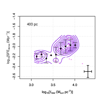
Figure 17: Star formation efficiency of the dense gas (SFE_dense) as a function of the stellar mass surface density ($\Sigma_{\rm star}$) in the SB ring of NGC 1068 at the ”initial resolution” (56 pc) (left panel), and at two averaging scales: 100 pc (middle panel) and 400 pc (right panel). Magenta circles and isodensity contours correspond to data measurements evaluated at the Nyquist-sampled grid of points after convolution with the appropriate Gaussian for each aperture. Black circles show median SFE_dense values and errorbars indicate the rms scatter in the bins. Symbols and isodensity contours in the middle panel identify the data obtained in other galaxies.The dashed orange line represents the fit of Usero et al. (2015). Vertical and horizontal errorbars at the lower right corner of each panel account for the typical uncertainties, which amount to $\pm 0.13$ dex and $\pm 0.09$ dex, respectively.

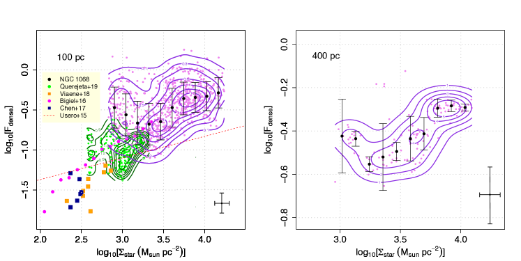
Figure 18: Fraction of dense gas ($F_{\rm dense}$) as a function of the stellar mass surface density ($\Sigma_{\rm star}$) in the SB ring of NGC 1068 at the two averaging scales: 100 pc (left panel) and 400 pc (right panel). Symbols as in Fig. 17. Vertical and horizontal errorbars at the lower right corner of each panel account for the typical uncertainties, which amount to $\pm 0.13$ dex and $\pm 0.09$ dex, respectively.

Figure 17 represents SFE_dense as a function of $\Sigma_{\rm star}$ across the SB ring of NGC 1068 for the three working apertures adopted in Sect. 6.1. SFE_dense does not show any significant correlation with $\Sigma_{\rm star}$ at the ”initial resolution” ($\rho_{\rm sp}=+0.10$, with a $p$-value $>1\%$), or at the 100 pc averaging scale ($\rho_{\rm sp}=+0.15$, with a $p$-value $>1\%$). On the contrary, SFE_dense shows a statistically significant positive correlation with $\Sigma_{\rm star}$ in the SB ring for $\Delta A=400$ pc ($\rho_{\rm sp}=+0.59$, with a $p$-value $<1\%$). We compare the location of NGC 1068 in the SFE_dense-$\Sigma_{\rm star}$ parameter space with the position occupied by the galaxies studied by the references listed in Table 8 in the middle panel of Fig. 17. NGC 1068 clearly deviates from the overall anti-correlation trend followed by other galaxies. The positive correlation observed in the NGC 1068 SB ring is in stark contrast with the anticorrelation trends identified in the galaxies studied by Usero et al. (2015) ($\rho_{\rm sp}=-0.50$), Querejeta et al. (2019) ($\rho_{\rm sp}=-0.57$), and Gallagher et al. (2018) ($\rho_{\rm sp}=-0.66$). In this context it is noteworthy that Querejeta et al. (2019) noticed that for a given value of $\Sigma_{\rm star}$ the data points of M 51 span a significant 1 dex range of SFE_dense, namely similar to the spread of values seen in the NGC 1068 SB ring. This is an indication of the wide range of dynamical environments probed in both galaxies.

Figure 18 represents $F_{\rm dense}$ as a function of $\Sigma_{\rm star}$ across the SB ring of NGC 1068 for the two averaging scales adopted in Sect. 6.1. $F_{\rm dense}$ shows already a significant correlation with $\Sigma_{\rm star}$ at $\Delta A=100$ pc ($\rho_{\rm sp}=+0.40$, with a $p$-value $<1\%$). The correlation is further reinforced when we use 400 pc as averaging scale ($\rho_{\rm sp}=+0.67$, with a $p$-value $<1\%$). This is qualitatively and quantitatively similar to the trends identified in the data of the galaxies shown in the left panel of Figure 18 at scales of 100 pc, for which Querejeta et al. (2019) derived a Spearman rank parameter of $\rho_{\rm sp}\sim+0.45$, and $\rho_{\rm sp}\sim+0.7$ when they added the datapoints from Chen et al. (2017) and Gallagher et al. (2018).

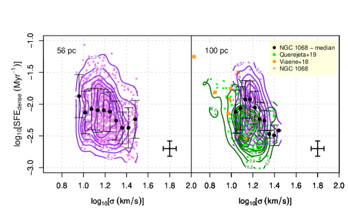
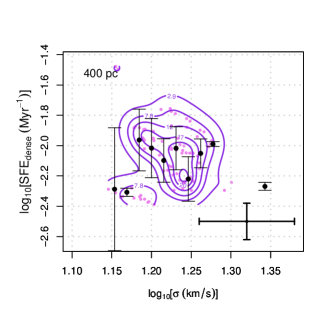
Figure 19: Star formation efficiency of the dense gas (SFE_dense) as a function of the velocity dispersion of HCN ($\sigma$) in NGC 1068 for three averaging scales: 56 pc (left panel), 100 pc (middle panel) and 400 pc (right panel). Measurements at 100 pc scales are compared to literature data for other galaxies. Symbols as in Fig. 17. Vertical and horizontal errorbars at the lower right corner of each panel account for the typical uncertainties, which amount to $\pm 0.13$ dex and $\pm 0.06$ dex, respectively.

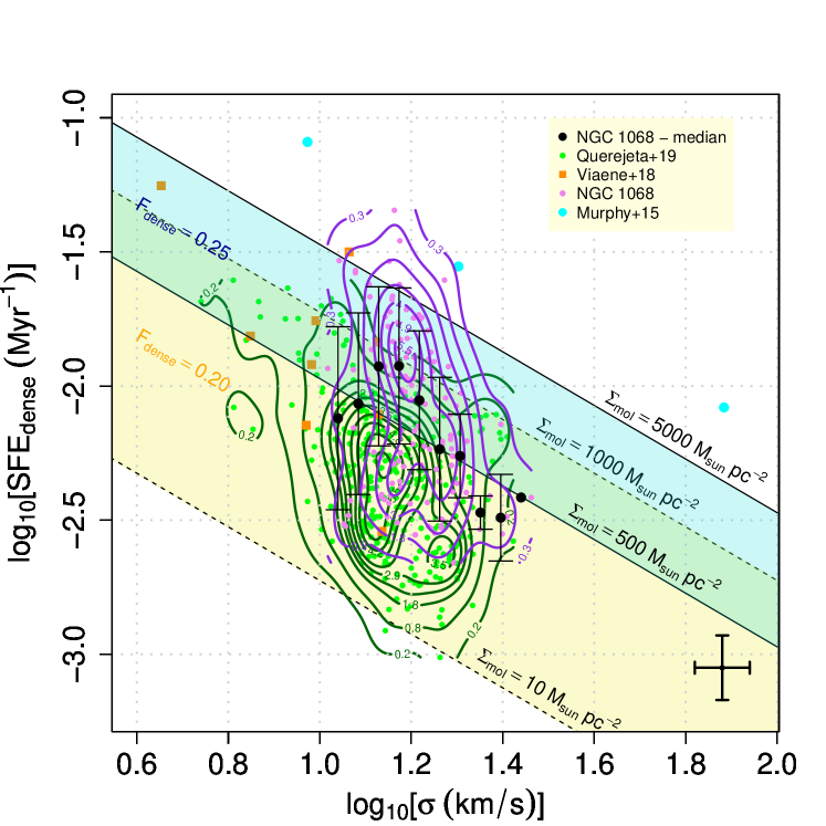
Figure 20: Same as the middle panel of Fig. 19 but adding a comparison with the trends of SFE_dense as a function of the velocity dispersion of the gas ($\sigma$) predicted by the model of Meidt et al. (2020). This model foresees different locations of galaxies in the SFE${}_{\rm dense}-\sigma$ parameter space depending on the fraction of dense gas ($F_{\rm dense}$) and, also, on the total molecular gas column densities ($\Sigma_{\rm mol}$). Symbols as in Fig. 17. Vertical and horizontal errorbars at the lower right corner account for the typical uncertainties, which amount to $\pm 0.13$ dex and $\pm 0.06$ dex, respectively.

Figure 21: Dense gas fraction ($F_{\rm dense}$) as a function of velocity dispersion in the SB ring of NGC 1068 at the two averaging scales: 100 pc (left panel) and 400 pc (right panel). Measurements at 100 pc scales are compared to literature data for other galaxies. Symbols as in Fig. 17. Vertical and horizontal errorbars at the lower right corner of each panel account for the typical uncertainties, which amount to $\pm 0.13$ dex and $\pm 0.06$ dex, respectively.

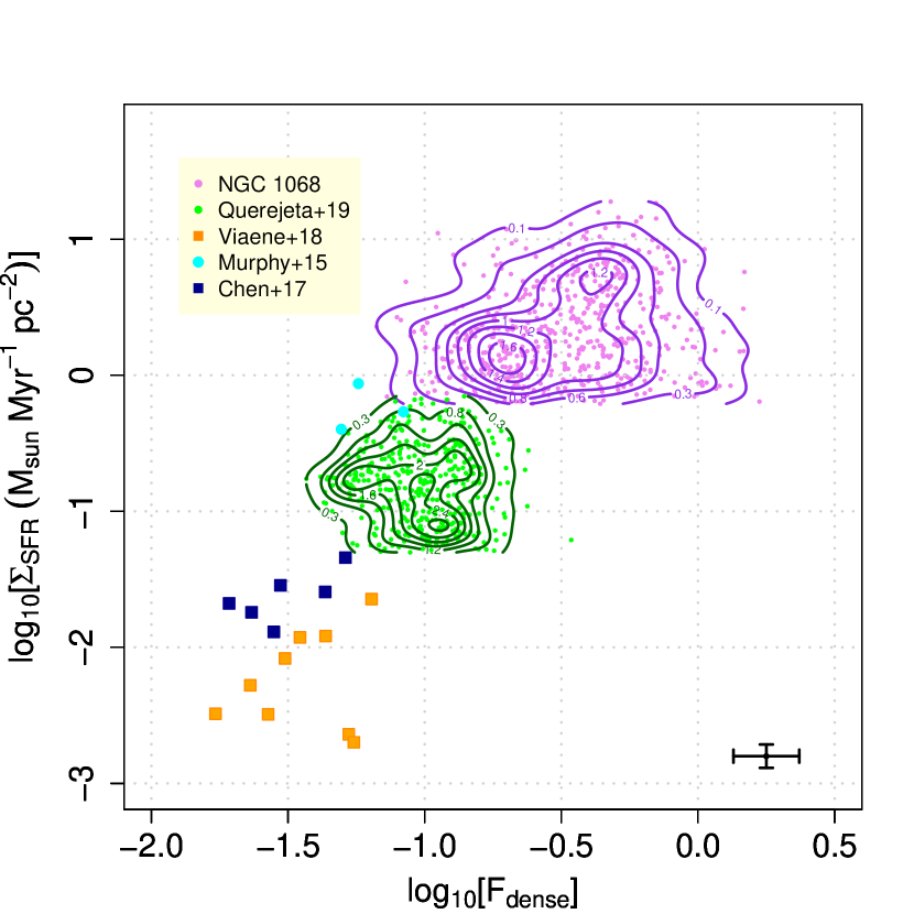
Figure 22: Star formation rate surface density ($\Sigma_{\rm SFR}$) as a function of dense gas fraction ($F_{\rm dense}$) in NGC 1068 measured at 100 pc scales compared to the data obtained in other galaxies (symbols as in Fig. 8). Vertical and horizontal errorbars at the lower right corner account for the typical uncertainties, which amount to $\pm 0.09$ dex and $\pm 0.13$ dex, respectively

.

6.4 Trends as a function of velocity dispersion

The role of velocity dispersion in setting the efficiency of molecular gas at forming stars is central to current models of turbulence-driven SF via their dependence on the Mach number (e.g., Krumholz & McKee, 2005; Hennebelle & Falgarone, 2012; Federrath, 2015). From the observational point of view, and under the hypothesis that the velocity dispersion measured at a given scale reflects mainly turbulent motions in molecular gas, identifying trends in SFE as a function of local velocity dispersion may indicate whether SF tends to be either enhanced or suppressed by turbulence. The predictions of models on the expected trends of SFE_dense as a function of the ”observed” velocity dispersion ($\sigma$) differ depending on the role of turbulence versus large-scale bulk motions (e.g., streaming motions) that are driven by the background gravitational potential. The degree of coupling to the large-scale gravitational potential implies that the critical threshold for star formation is not universal and that SFE_dense is therefore not constant. Specifically, the recent model published by Meidt et al. (2020) foresees that SFE_dense should decrease with $\sigma$ at fixed values of $F_{\rm dense}$ and $\Sigma_{\rm mol}$.

Leroy et al. (2017) found a decreasing trend between the efficiency of the bulk molecular gas (SFE_mol) and $\sigma$ measured from CO(1–0) in M 51. Querejeta et al. (2019) also found a significant anti-correlation between SFE_dense and $\sigma$ in M 51 ($\rho_{\rm sp}=-0.62$). A comparison of the observations of M 31 (Viaene et al., 2018) and M 51 (Querejeta et al., 2019) with the predictions of Meidt et al. (2020)’s model shows a fair agreement for apertures of 100 pc.

Figure 19 examines the trends in SFE_dense as a function of $\sigma$ across the SB ring of NGC 1068 for the three apertures adopted in Sect. 6.1. We note that the value of $\sigma$ derived on scales of 56 pc is not a good proxy for the ”internal” turbulence of the dense cores probed by HCN, which in all likelihood have sizes $\sim$a few pc. Instead, $\sigma$ likely encapsulates a mix of the ”macroscopic” turbulence between the cores and the residual gradient of large-scale bulk motions within the ALMA beam. The correlation shown in Fig. 19 is not statistically significant for the two extreme values of the averaging apertures (56 pc and 400 pc). However, there is a weak yet significant trend at 100 pc scales, for which we derive a $\rho_{\rm sp}=-0.28$, with a $p$-value $=0.3\%$. Overall, the results obtained in NGC 1068 show a very marginal agreement with the results of Viaene et al. (2018) and Querejeta et al. (2019) and, therefore, with the predictions of Meidt et al. (2020)’s model. As illustrated in Fig. 20, a fraction of the data corresponding to the SB ring in NGC 1068 lies in the region predicted by Meidt et al. (2020) for $F_{\rm dense}\sim 0.25$ and a range for $\Sigma_{\rm mol}\sim 500-5000\leavevmode\nobreak\ M_{\sun}$pc^-2. Although these values are in rough agreement with the ones estimated for a high fraction of the SB ring positions, the decreasing trend in SFE_dense as a function of $\sigma$ is seen to be much shallower than the one predicted by Meidt et al. (2020). However, as noted by Meidt et al. (2020), a gravitational potential linked to a strong density wave (bar or spiral) may tend to degrade the strength of the expected decreasing trend, which is estimated in their model using a purely axisymmetric disk.

Figure 21 explores the trends of $F_{\rm dense}$ as a function of $\sigma$ in the SB ring for the two averaging scales adopted in Sect. 6.1. In contrast with the trends identified in M 31 and M 51 by Viaene et al. (2018) and Querejeta et al. (2019) on 100 pc scales, $F_{\rm dense}$ fails to show any significant correlation with $\sigma$ in the SB ring of NGC 1068 for $\Delta A=100$ pc ($\rho_{\rm sp}=+0.10$, with a $p$-value $>1\%$), However, a significant positive trend appears when we use 400 pc as averaging scale ($\rho_{\rm sp}=+0.50$, with a $p$-value $<1\%$).

6.5 Relation between the star formation rate and the dense gas fraction

Viaene et al. (2018) observed a significant correlation ($\rho_{sp}=0.63$) between the SFR and $F_{\rm dense}$ in a number of regions in the disk of M 31 observed with a spatial resolution of 100 pc. Querejeta et al. (2019) explored the correlation between $\Sigma_{\rm SFR}$ and $F_{\rm dense}$ in M 51 after incorporating the data obtained by Chen et al. (2017) in M 51 on similar spatial scales and derived a similar positive trend: $\rho_{\rm sp}=0.63$, with a $p$-value $<1\%$. This correlation improved when Querejeta et al. (2019) included the M 31 and NGC 3627 data of Viaene et al. (2018) and Murphy et al. (2015), respectively ($\rho_{\rm sp}=0.66$).

Figure 22 shows the region occupied by the NGC 1068 data in the $\Sigma_{\rm SFR}$–$F_{\rm dense}$ plot for an adopted averaging scale $\Delta A=100$ pc. We do not find a strong correlation between $\Sigma_{\rm SFR}$ and $F_{\rm dense}$ ($\rho_{\rm sp}$=0.22) when we consider the NGC 1068 data alone. In particular, this correlation is weaker than the one found between $\Sigma_{\rm SFR}$ and $\Sigma_{\rm dense}$ for the same spatial scales ($\rho_{\rm sp}$=0.35; see Table 6). This result is an indication that the dense gas fraction is not a better predictor of star formation than the dense gas content in the SB ring. However, if we include the data published for the galaxies displayed in Figure 22, the overall correlation improves significantly ($\rho_{sp}$=0.72). Querejeta et al. (2019) used all the available data at 100 pc scales and similarly concluded that the dense gas fraction does not seem to be a better predictor of the SFR surface density than the dense gas surface density.

7 A scenario for star formation in the SB ring

The results of our work support the relevance of dynamical environment in setting the efficiency of SF of the dense molecular gas in galaxy disks. Specifically, we find that SFE_dense is comparatively boosted by up to a factor of three to four in the bar-ring interface of NGC 1068 relative to the regions located elsewhere in the ring.

The velocity dispersion of the dense gas as derived from the HCN(1–0) line at the ”initial resolution” of ALMA shows little variations over the SB ring. For an averaging scale of 400 pc, Fig. 23 shows that $\sigma$ changes from $\sim 14$ to $\sim 19$ km s^-1 with an estimated mean value of about 16 km s^-1 . Specifically, $\sigma$ shows only a moderate $\sim 30\%$ increase in the southern region of the bar-ring interface (see Fig. 23). This is in agreement with the picture drawn from the analysis of the velocity dispersion estimated at 42 pc resolution from the CO(3–2) line, as illustrated by Fig 10 of García-Burillo et al. (2014). Furthermore, the right panel of Fig. 21 shows that, while $F_{\rm dense}$ increases by $\sim 0.6$ dex, the corresponding increase in $\sigma$ ($\sim 0.12$ dex) is a factor of three smaller. Although $F_{\rm dense}$ and $\Sigma_{\rm dense}$ are not identical quantities, the superlinear trend of $F_{\rm dense}$ as a function $\sigma$ implies that the trends in the boundedness parameter described in Sect. 6.1 are mostly driven by the observed boost in $F_{\rm dense}$ in the bar-ring interface. All in all, these results suggest that molecular gas undergoes an efficient compression likely as a result of an enhanced rate of cloud-cloud collisions in the bar-ring interface. However, the shallow trends in $\sigma$ suggest that cloud-cloud collisions have not increased to any significant level the ”macroscopic” turbulence between the cores of dense gas probed on scales of 56 pc in this region.

The SB ring is formed by a tightly wound two-arm spiral structure. The gas accumulates in a region where two density-wave resonances are thought to be overlapping: the inner Lindblad resonance (ILR) of the $\sim 17$ kpc-size outer stellar oval and the corotation of the $\sim 2.6$ kpc-diameter stellar bar (Bland-Hawthorn et al., 1997; Schinnerer et al., 2000; Emsellem et al., 2006). The accumulation of gas at the SB ring suggests that the barrier imposed by the corotation of the (nuclear) stellar bar has been overcome . This could reflect either the influence of the outer stellar oval, which produces gas inflow down to its ILR, or alternatively, the influence of a decoupled (lower pattern speed) spiral mode, which would also induce gas inflow inside its own corotation. Based on a Fourier decomposition of streaming motions derived from CO(3–2), García-Burillo et al. (2014) found the signature of systematic gas inflow across the SB ring, an indication that the two-arm spiral constitutes an independent wave feature characterised by a lower pattern speed. The inward motions detected are particularly strong at the region connecting the bar with the spiral (see Fig. 14 of García-Burillo et al., 2014). In either case, orbital crowding and the intersection of molecular gas on the orbits of the bar and the spiral are seen to enhance SFE_dense in their interface region. Rico-Villas et al. (2021) recently analysed the continuum emissions at 147 and 350 GHz observed with ALMA, together with the Pa$\alpha$ HST/NICMOS image of NGC 1068, and identified 14 super star clusters (SSC) in the SB ring. In agreement with the scenario described above, most of the SSCs (11 out of 14) are seen to be located at the bar ends.

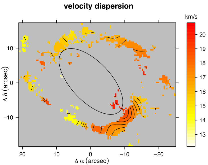
Figure 23: Same as Fig. 12 but showing the map of the velocity dispersion ($\sigma$) obtained using 400 pc as averaging scale. Contour levels for $\sigma$ go from 14.0 to 19.0 in steps of 0.5 km s^-1.

NGC 1068 is not by any means an isolated case that illustrates how the complex molecular gas dynamics in a bar-spiral arm interface can trigger SF activity in a galaxy disk. In particular, Beuther et al. (2012) found evidence that the particular dynamical environment of the W43 mini-starburst complex in the Milky Way has likely increased cloud interactions and the subsequent SF activity in this region, which is located near the Galactic bar-spiral arm interface. Furthermore, Beuther et al. (2017), and more recently, Bešlić et al. (2021) found an increase of SF activity in the bar-spiral arm interface region of the strongly barred galaxy NGC 3627, as a result of the accumulation of gas where the two orbit families (related to the bar and the spiral) intersect, triggering cloud-cloud collisions. Specifically, the work of Bešlić et al. (2021) reveals that, compared to other regions in the disk of NGC 3627, the efficiency of the dense molecular gas derived from H$\alpha$/HCN ratios is significantly enhanced in the bar-spiral arm interface region. Similarly to the scenario described by Beuther et al. (2017) for NGC 3627, we conclude that a configuration where the bar and spiral may rotate at two different pattern speeds can explain the intense star formation at the bar-ring interface of NGC 1068.

Several hydrodynamical numerical simulations have investigated the role of large-scale bars in AGN fueling and in triggering SF in galaxy disks (e.g.; Renaud et al., 2013, 2015; Emsellem et al., 2015). In particular, Renaud et al. (2015) showed that the SFE and the formation of massive stellar associations are enhanced at the extremities of the bar to a level comparable to the one observed in galaxy-galaxy interactions as a result of cloud-cloud collisions. This scenario seems to account for the observed pattern of SFE_dense in NGC 1068.

8 Summary and conclusions

We used ALMA to image the emission of dense molecular gas in the $r\sim 1.3$ kpc SB ring of the Seyfert 2 galaxy NGC 1068 with a resolution of $\sim 56$ pc using the 1–0 transitions of HCN and HCO⁺. We also used ancillary data of CO (1–0), as well as CO(3–2) and its underlying continuum emission at the resolutions of $\sim 100$ pc and $\sim 40$ pc, respectively. These observations allow us to probe a wide range of molecular gas densities ($n_{\rm H_{2}}\sim 10^{3-5}$cm^-3). The SF rate is derived from Pa$\alpha$ line emission imaged by HST/NICMOS. We analysed the influence of the dynamical environment on different formulations of SF relations in the SB ring and compared our results with the general predictions of density-threshold and turbulent SF models.

The main results of this paper are summarized as follows:

• We derived spatially resolved KS laws for a set of seven spatial resolutions, ranging from $\sim 40$ pc up to $\sim 700$ pc. We studied how these relations change depending on the adopted aperture sizes and on the choice of molecular gas tracer. For a given spatial resolution the correlation parameters derived from the high density tracers (CO(3–2), HCN(1–0) and HCO⁺(1–0)) are about a factor of two to three larger than that derived from CO(1–0).

• The KS correlations lose statistical significance below a critical spatial scale $\approx$ 300-400 pc common for all gas tracers. For spatial scales $\geq 300-400$ pc the correlation improves monotonically as a function of the aperture size for all gas tracers excluding CO(1–0). While dust continuum emission shows a behaviour similar to the rest of high density tracers, the dust-based KS correlation is significant already at 100 pc scales.

• NGC 1068 lies within the general $\Sigma_{\rm SFR}$–$\Sigma_{\rm dense}$ linear KS relationship derived from a compilation of data obtained in other galaxies. In particular, the location of NGC 1068 in the KS plot is intermediate between the one of normal galaxies and (U)LIRG, a result that underlines the relatively extreme conditions in the SB ring.

• The efficiency of SF of the dense molecular gas, defined as SFE${}_{\rm dense}\equiv\Sigma_{\rm SFR}/\Sigma_{{\rm dense}}$, shows a scattered distribution as a function of the HCN luminosity at the ”initial resolution” of ALMA ($\sim 56$ pc) around a mean value of $\simeq 0.01$Myr^-1. However, we find evidence of a significant environmental dependence of SFE_dense reflected in the existence of systematic trends across the different regions of the SB ring, which are inconsistent with the predictions of density-threshold models.

• With the aim of resolving the degeneracy associated with the SFE_dense-$L^{\prime}$(HCN) plot, we explored an alternative prescription for SF relations, which includes the dependence of SFE_dense on the boundedness of the gas, measured by the parameter $b$ defined as $b\equiv\Sigma_{\rm dense}/\sigma^{2}\propto\alpha_{\rm vir}^{-1}$. We identified two branches in the version of the SFE_dense–$b$ plot derived for an averaging scale of 400 pc. The two branches correspond to two dynamical environments defined by their proximity to the region where the SB ring is connected to the stellar bar of NGC 1068.

• We studied the trends in SFE_dense as a function of the dense gas fraction ($F_{\rm dense}$), the stellar mass surface density ($\Sigma_{\rm star}$), and the velocity dispersion ($\sigma$) in the SB ring using different averaging scales. We find that SFE_dense correlates both with $F_{\rm dense}$ and $\Sigma_{\rm star}$. However, we find no significant correlation of SFE_dense with $\sigma$. These results differ to a large extent from those derived from previous kpc-scale studies of galaxy disks and high-resolution ($\sim 100$ pc) observations of M 51.

• The trends in the boundedness parameter in the SB ring are mostly driven by the observed boost in $F_{\rm dense}$ in the bar-ring interface region. The results reflect a significant compression of molecular gas as a result of an enhanced rate of cloud-cloud collisions in the bar-ring interface on the one hand, and an efficient dissipation of turbulence on the other.

The outcome of our work emphasizes the relevance of different dynamical environments to modulating SFE_dense in galaxy disks. Taken at face value, this result is inconsistent with the predictions of density-threshold models, which foresee the existence of a nearly constant canonical value for SFE_dense. There is mounting observational evidence that SFE_dense can show systematic trends based on studies carried out both in our Galaxy and nearby galaxies. However, the theoretical scenarios advanced to explain the variations of SFE_dense reported in the literature are diverse. This diversity reflects the variety of trends observed in SFE_dense as a function of key physical variables such as $F_{\rm dense}$, $\Sigma_{\rm star}$, and $\sigma$ in galaxy disks. Similarly to the case of the barred galaxy NGC 3627 discussed by Beuther et al. (2017), the enhanced SF activity in the bar-ring interface of NGC 1068 could be explained by a dynamical configuration in which the bar and the two-arm spiral feature are independent $m=2$ modes rotating at different pattern speeds. Further studies are required to explore the frequency of this type of dynamical decoupling between bars and spirals and their role at setting the SF efficiency of dense molecular gas in galaxy disks in general and in galactic rings in particular.

Appendix A Determination of the missing flux in HCN and CO maps

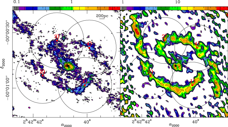
Figure 24: Left panel: Overlay of the four $\sim 30\arcsec$-size apertures (black circles, identified by the numerical labels 1-4) selected to cover the SB ring of NGC 1068 on the ALMA HCN(1–0) map (colour scale and contours as in Fig. 1), used in Appendix A to estimate the missing flux correction. Right panel: same as left panel but showing the overlay of the four $\sim 12\arcsec$-size apertures (black circles, identified by the numerical labels 1-4) selected to cover the SB ring of the galaxy on the PdBI CO(1–0) map of Schinnerer et al. (2000). Colour scale is given in Jy km s^-1 beam^-1 units and the position of the AGN is identified by the grey star markers in both maps. The (magenta) filled ellipses at the bottom left in the two panels represent the beam sizes.

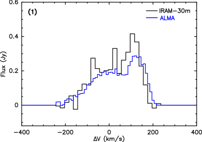
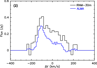
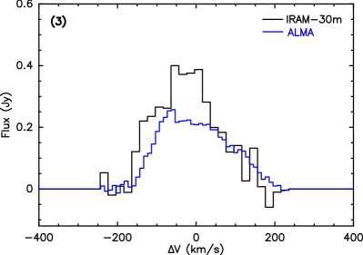
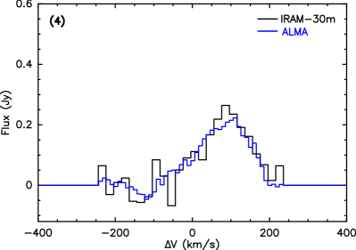
Figure 25: Comparison of the HCN(1–0) emission observed by ALMA (blue histograms) and the IRAM-30m telescope (black histograms) inside the four selected regions identified in Fig. 24 (labelled as 1, 2, 3, and 4 in each panel).

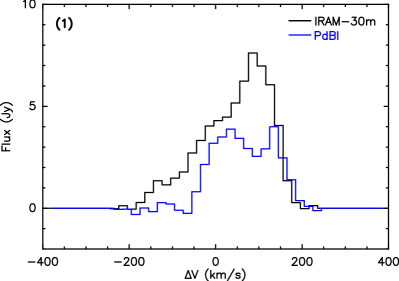
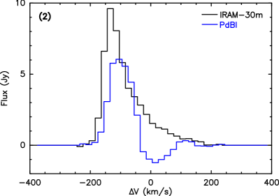
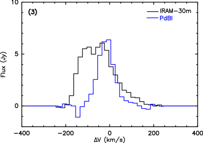
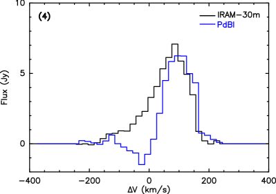
Figure 26: Same as Fig. 25, but showing the comparison of the CO(1–0) emission observed by the IRAM-PdBI (blue histograms) and the IRAM-30m telescope (black histograms) inside the four selected regions identified in Fig. 24 (labelled as 1, 2, 3, and 4 in each panel).

We estimated the missing flux in the HCN(1–0) map obtained by ALMA and in the CO(1–0) map of the IRAM array (PdBI) (Schinnerer et al. 2000). To this aim, we measured the spatially-integrated fluxes in both lines using a set of four apertures covering the region occupied by the SB ring of NGC 1068. The interferometer fluxes are compared with the corresponding single-dish fluxes measured from observations obtained by the IRAM-30m telescope (Usero et al., private communication). Figure 24 illustrates the apertures chosen overlaid on the HCN (left panel) and CO (right panel) interferometer images of the galaxy. The sizes of the apertures used to derive the spatially-integrated fluxes of the interferometer maps correspond to the single-dish beams of the IRAM-30m telescope, which are $\sim 30\arcsec$ and $\sim 24\arcsec$ for HCN and CO, respectively.

Figures 25 and 26 compare the spectra of HCN and CO obtained by integrating the emission of the lines inside the four selected regions shown in Fig. 24 with the IRAM-30m spectra. Based on this comparison we estimate that on scales of $\sim 30\arcsec$ ($\sim 2$ kpc) approximately $20-25\%$ of the total flux gets filtered in the HCN ALMA map. A similar estimate for the CO map yields a flux filtering of about 40-45$\%$ on scales $\sim 24\arcsec$ ($\sim 1.7$ kpc). This is about a factor of two larger than the value estimated by Schinnerer et al. (2000), who compared the fluxes measured with the PdBI with those measured with the combined BIMA array and Kitt Peak single-dish telescope datasets on scales $\sim 55\arcsec$ (3.8 kpc).

As in this paper we analyse spatial scales that are much smaller than the critical scales reported above ($\thickapprox$ 2-4 kpc), we can foresee that the missing flux factors will be significantly less than 25-45$\%$ for the scales that are relevant to our study.

Appendix B Pa$\alpha$ analysis as SFR tracer

To validate our working assumption, namely that the Pa$\alpha$ image used in this work to derive the distribution of recent SF in NGC 1068 does not require a significant correction by dust extinction, we compared the Pa$\alpha$ fluxes measured in the HST/NICMOS image of the galaxy with the H$\alpha$ fluxes measured using the ground-based image of Díaz et al. (2000) over a representative number of hot spots of the SB ring. Figure 27 shows the position of the eight regions considered in this comparison selected from Table 4 of Díaz et al. (2000). We derived the Pa$\alpha$ spatially-integrated fluxes inside the eight selected regions using the sizes of H$\alpha$ SF knots listed in Table 4 of Díaz et al. (2000) and obtained the H$\alpha$/Pa$\alpha$ flux ratios for each aperture (listed in Table 17). To estimate the colour excess ($E(B-V)$) and extinction (A_Paα) values we used the prescriptions of Calzetti (2001) (see also Calzetti et al. 1994, 2000) and the standard equation:

$$F_{\rm obs}(\lambda)=F_{\rm int}(\lambda)10^{-0.4k(\lambda)E(B-V)},$$ (12)

where $F_{\rm obs}$ and $F_{\rm int}$ are the observed and intrinsic fluxes for the lines, respectively, and $E(B-V)$ is the colour excess. We assumed that the differential extinction between the two lines is determined by $k(H\alpha)-k(Pa\alpha)=2.104$ (Calzetti 2001). Table 17 lists the H$\alpha$/Pa$\alpha$ line ratios as well as the values estimated for $E(B-V)$ and A_Paα for the eight selected regions.

The median value for the distribution of H$\alpha$/Pa$\alpha$ ratios listed in Table 17 is $\sim 6.8$. The latter is close to the expected value corresponding to the canonical case B recombination: $\sim 7.8$. The implied mean extinction correction at 1.875 $\mu$m is A_Paα=0.03 mag, which translates into very low dust opacities for the ensemble of the studied SF knots. Although in regions 18,19 and 20, A_Paα is seems to reach values $\sim 0.1-0.2$, the implied opacities are still compatible with optically thin emission for Pa$\alpha$. Moreover, assuming that the flux scale is uncertain to $\pm$ 20$\%$ due to absolute calibration errors, we can therefore conclude that Pa$\alpha$ emission is not significantly affected by dust extinction in the SB ring of NGC 1068.

Region	H$\alpha$/Pa$\alpha$	E(B-V) [mag]	APaα [mag]
1	7.7	0.01	$\leq$ 0.01
3	9.9	-0.12	-0.05
4	7.7	0.01	$\leq$ 0.01
8	9.0	-0.07	-0.03
10	5.9	0.15	0.05
18	3.8	0.37	0.14
19	2.1	0.67	0.24
20	3.5	0.41	0.15
median	6.8	0.08	0.03

Table 4: Observed line ratios and derived extinction parameters for the SB ring knots of NGC 1068.

Figure 27: HST/NICMOS Pa$\alpha$ image of NGC 1068. The (white) labels identify the regions selected to estimate the extinction of Pa$\alpha$, according to the nomenclature used by Díaz et al. (2000).

Appendix C Kennicutt-Schmidt plots

We represent the Kennicutt-Schmidt plots derived from the different tracers for the range of scales used in this work (Figures 28, 29, 30 and 31).

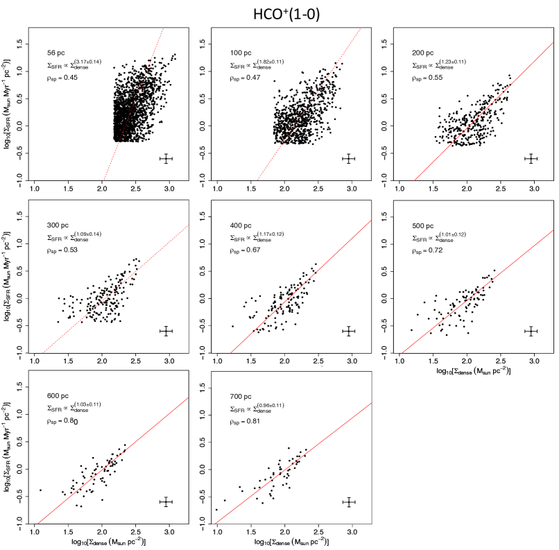
Figure 28: Same as Fig. 5, but showing all the spatial scales used in this work for HCO⁺(1-0). Vertical and horizontal errorbars at the lower right corner of each panel account for the typical uncertainties, which amount to $\pm$0.09 dex on both axes.

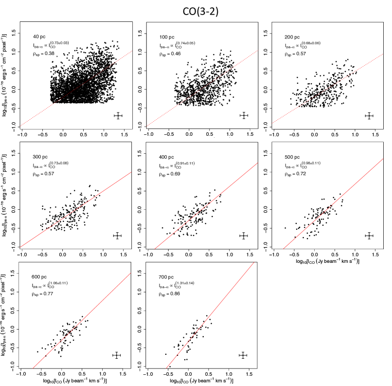
Figure 29: Same as Fig. 5, but showing all the spatial scales used in this work for CO(3-2). Vertical and horizontal errorbars at the lower right corner of each panel account for the typical uncertainties, which amount to $\pm$0.09 dex on both axes.

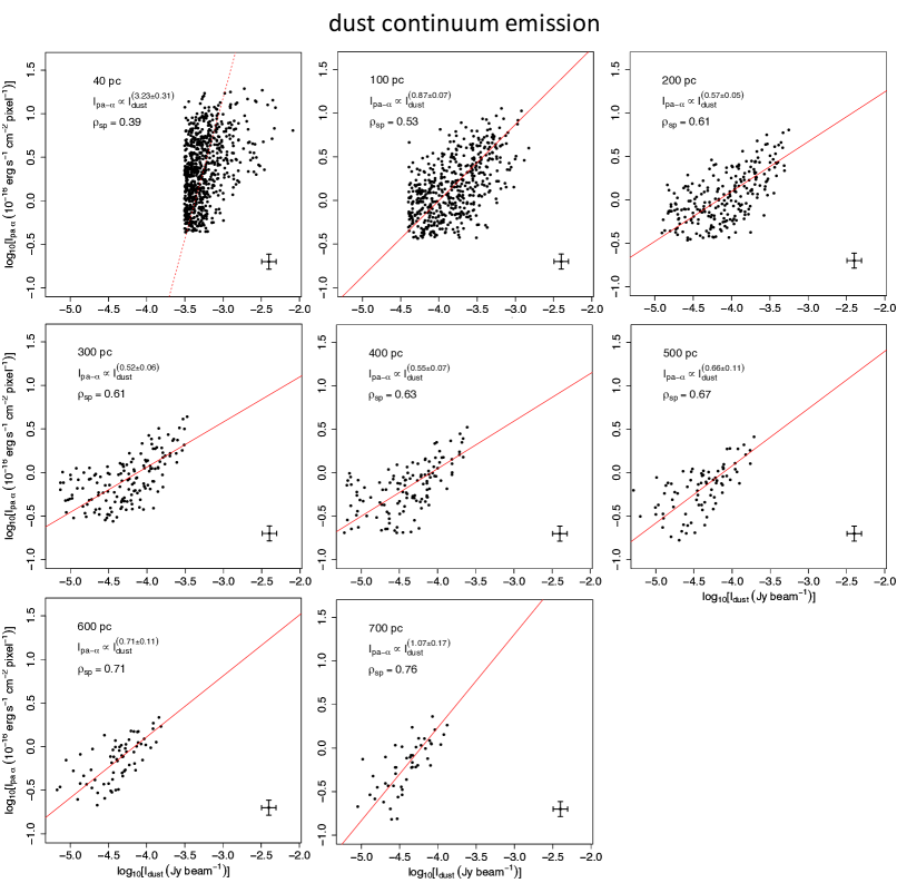
Figure 30: Same as Fig. 5, but showing all the spatial scales used in this work for dust continuum emission. Vertical and horizontal errorbars at the lower right corner of each panel account for the typical uncertainties, which amount to $\pm$0.09 dex on both axes.

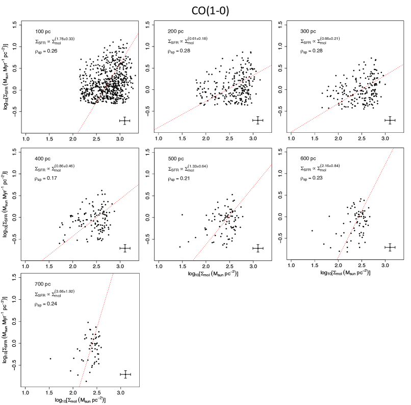
Figure 31: Same as Fig. 5, but showing all the spatial scales used in this work for CO(1-0). Vertical and horizontal errorbars at the lower right corner of each panel account for the typical uncertainties, which amount to $\pm$0.09 dex and $\pm$0.10 dex, respectively.

Appendix D Alternative formulation of the intensity-weighted average of the $b$ parameter

Leroy et al. (2017) used a definition of the intensity-weighted average of the $b$ parameter different to the one used in Sect 6.1. In particular, instead of deriving the averages of $b$ as defined in Eq. 10, they performed the averages of $\Sigma_{\rm gas}$ and $\sigma^{2}$ separately and defined : $\langle b\rangle\equiv\langle\Sigma_{\rm gas}\rangle/\langle\sigma^{2}\rangle$. We have derived a new version of Fig. 11 using the definition of Leroy et al. (2017) particularized for $\Sigma_{\rm dense}$ and our set of two apertures (100 pc and 400 pc). The results obtained with this definition, shown in Fig. 32 are virtually identical to those shown in Fig. 11. In particular, we obtain (anti) correlation Spearman rank parameters $\rho_{\rm sp}=-0.42$ and $-0.60$ for $\Delta A=100$ pc and $400$ pc, respectively, and associated two-sided $p$-values $<1\%$. Furthermore, after applying the MARS routine to the 400 pc-scale scatter-plot we find a turnover at log₁₀($\langle b\rangle$)$=0.18\leavevmode\nobreak\ M_{\sun}$pc^-2(km s^-1)^-2 and a slope $\simeq-1.4$ for $\langle b\rangle$ values beyond the turnover.

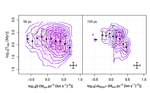
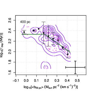
Figure 32: Same as Fig. 11 but derived using the alternative formulation of the intensity-weighted average of the $b$ parameter used by Leroy et al. (2017).

Appendix E Trends as a function of the boundedness of the gas from HCO⁺

We have studied in Sect. 6.1 how the depletion time of the dense molecular gas estimated from HCN changes as a function of the self-gravity of the gas ($b$ $paramater$). We now analyse this with the other dense gas tracer that we use in this work, HCO⁺. Figure 33 represents the depletion time as a function of the $b$ parameter at 56 pc, 100 pc and 400 pc. We observe a similar trend to Figure 11, obtaining (anti) correlation Spearman rank paramaters $\rho_{sp}$ = -0.07 (p-value = 0.06), -0.32 (¡1$\%$) and -0.65 (¡1$\%$) for 56 pc, 100 pc and 400 pc, respectively. At 400 pc scales, we identify a turnover in the plot located around log₁₀($\langle b\rangle$) $\simeq$ 0.2 $M_{\sun}$pc^-2(km s^-1)^-2 and a slope $\simeq$ -0.91 for $\langle b\rangle$ values beyond the turnover.

Figure 33 shows the spatial distribution of $T_{dep}^{dense}$ and $\langle b\rangle$ derived for $\Delta A$ = 400 pc in the SB ring of NGC 1068 from HCO⁺. We observe that higher (lower) SFE_dense ($T_{dep}^{dense}$) values are located closer to the bar-ring interface. We find that the HCN and HCO⁺ show similar correlations in the SB ring of NGC 1068.

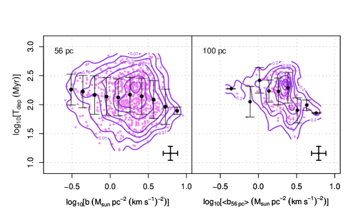
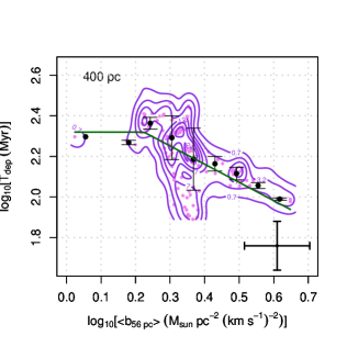
Figure 33: Same as Fig. 11 but estimated from HCO⁺.

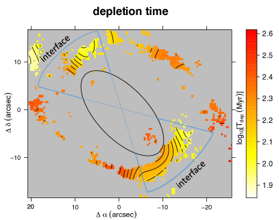
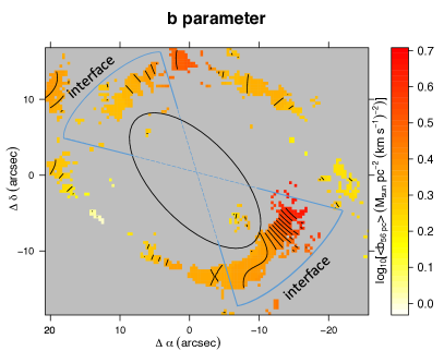
Figure 34: Same as Fig. 12 but estimated from HCO⁺. $Left$ $panel$: contour levels for log₁₀($T_{dep}^{dense}$) go from 1.90 to 2.50 in steps of 0.045 (in Myr). $Right$ $panel$: contour levels for log₁₀($\langle b\rangle$) go from 0.02 to 0.64 to 0.025 (in M_⊙pc^-2(km s^-1)^-2).