INTENSITY AND POLARIZATION CHARACTERISTICS
OF EXTENDED NEUTRON STAR SURFACE REGIONS

Abstract

The surfaces of neutron stars are sources of strongly polarized soft X rays due to the presence of strong magnetic fields. Radiative transfer mediated by electron scattering and free-free absorption is central to defining local surface anisotropy and polarization signatures. Scattering transport is strongly influenced by the complicated interplay between linear and circular polarizations. This complexity has been captured in a sophisticated magnetic Thomson scattering simulation we recently developed to model the outer layers of fully-ionized atmospheres in such compact objects, heretofore focusing on case studies of localized surface regions. Yet, the interpretation of observed intensity pulse profiles and their efficacy in constraining key neutron star geometry parameters is critically dependent upon adding up emission from extended surface regions. In this paper, intensity, anisotropy and polarization characteristics from such extended atmospheres, spanning considerable ranges of magnetic colatitudes, are determined using our transport simulation. These constitute a convolution of varied properties of Stokes parameter information at disparate surface locales with different magnetic field strengths and directions relative to the local zenith. Our analysis includes full general relativistic propagation of light from the surface to an observer at infinity. The array of pulse profiles for intensity and polarization presented highlights how powerful probes of stellar geometry are possible. Significant phase-resolved polarization degrees in the range of 10-60% are realized when summing over a variety of surface field directions. These results provide an important background for observations to be acquired by NASA’s new IXPE X-ray polarimetry mission.

1 Introduction

The quasi-thermal soft X-ray emission from isolated pulsars and accreting neutron stars provides paths to understanding their surfaces and interiors. The surface temperature distribution can provide clues to the thermal conductivity of the upper crust and help inform magneto-thermal evolutionary models (e.g., Viganò et al., 2013). The intensity and polarization signals that are propagated to an observer at infinity are convolutions of local radiation anisotropies that depend on the global magnetic field structure of the surface. Such signals likely also depend on whether fully or partially-ionized atmospheres (Shibanov et al., 1992; Pavlov et al., 1994; Zane et al., 2000; Potekhin et al., 2004; Suleimanov et al., 2009) or condensates (Medin & Lai, 2006, 2007) constitute the outermost layers of the neutron star.

The periodic time traces of soft X-ray intensity provide powerful diagnostics on the sizes and locales of hot spots, and also on the angles between the magnetic axis and the observer viewing direction to the spin axis. Gotthelf et al. (2010) used such pulse profiles in a study of PSR J0821-4300 in the supernova remnant Puppis A. Employing a general relativistic (GR) propagation model, Perna & Gotthelf (2008) interpreted the pulse profiles of the magnetar XTE J1810-197 using a concentric ring polar hot spot that locally emitted blackbody radiation; they parameterized the radiation anisotropy, constraining the stellar geometry and mass-to-radius ratio somewhat, yet not profoundly. Albano et al. (2010) carried out Monte Carlo simulations of spectra and pulse profiles to constrain the geometric parameters for two transient magnetars XTE J1810-197 and CXOU J164710.2-455216 in the context of the globally-twisted magnetosphere model. Their flat spacetime analysis concluded that XTE J1810-197 is a moderately aligned rotator, with an angle $\,\alpha\sim 15^{\circ}-30^{\circ}\,$ between the magnetic and rotation axes, and a large observer angle $\,\zeta\sim 150^{\circ}\,$ to the spin axis. In contrast, they determined that CXOU J164710.2-455216 was an almost orthogonal rotator. Bernardini et al. (2011) performed a similar analysis with parameterized radiation anisotropy for XTE J1810-197 by fully including GR light bending and obtained somewhat larger magnetic obliquities $\,\alpha\sim 30^{\circ}-50^{\circ}\,$, and $\,\zeta\sim 20^{\circ}-50^{\circ}\,$. More recently, Younes et al. (2020) performed flat spacetime simulations with anisotropic emission to constrain the hot spots’ geometry for the flaring activity from the magnetar 1RXS J1708-40, obtaining $\,\alpha\sim 60^{\circ}\,$ and $\,\zeta\sim 60^{\circ}\,$.

The use of pulse profiles as probes of stellar parameters for other types of neutron stars has been extensive over the years. Riffert & Mészáros (1988) explored pulse profiles for accreting X-ray binaries as a means of discriminating between pencil beam and fan beam accretion pictures pertaining to columns of plasma inflow and surface impact hot spots. A similar approach also using the Schwarzschild metric was adopted by Harding & Muslimov (1998) as a path to constraining the $\,\alpha\,$ and $\,\zeta\,$ angles for middle-aged, isolated pulsars. Braje et al. (2000) studied Doppler boosting, Shapiro time delays and frame dragging influences of the Kerr metric in millisecond pulsar (MSP) contexts. Psaltis et al. (2014) addressed such GR influences in seeking paths to constrain the mass-to-radius ratio of these rapidly rotating neutron stars, which have served as core science deliverables for NASA’s Neutron Star Interior Composition Explorer (NICER) telescope: see Riley et al. (2019); Miller et al. (2019) for surface “hot spot” constraints for MSP J0030+0451.

The addition of polarization to the suite of neutron star diagnostics enhances the understanding of the source magnetic geometry. This observational prospect is on the near horizon given the very recent launch of the Imaging X-ray Polarimetry Explorer (IXPE) mission(Weisskopf et al., 2016) late in 2021. Polarized X-ray emission from neutron stars has been explored in numerous previous theoretical studies. For the context of accreting X-ray pulsars, the reader can survey the papers of Ventura, Nagel, & Mészáros (1979); Mészáros & Bonazzola (1981); Mészáros et al. (1988) and various articles cited in the book by Mészáros (1992) to discern the varied energy-dependent polarization signatures that define powerful observational probes of accretion geometry. This is generally the domain of hard X-ray polarimetry, and an introductory demonstration of diagnostic capability in this band was recently provided by the X-Calibur polarization measurement above 15 keV for the X-ray binary GX 301-2 (Abarr et al., 2020).

Ionized atmosphere models for magnetars constructed by Özel (2001) and Ho & Lai (2001) and a number of later papers generated polarization-dependent spectra by solving the radiative transfer equations for two photon normal modes, treating scattering and free-free absorption. Using a sophisticated treatment of the mode conversion at the vacuum resonance deeper down in the atmosphere, van Adelsberg & Lai (2006) calculated the polarization signatures from a magnetar hotspot. These and other studies predicted a predominance of the extraordinary ($\,\perp\,$) mode polarization because it emerges from deeper in the atmosphere, where the plasma is hotter so that thermal photons are more numerous. Magnetospheric propagation of polarized light in the birefringent quantum magnetized vacuum is also a key influence (Fernández & Davis, 2011; Taverna et al., 2020) in assessing the net polarization signals from magnetars. As a magnetospheric application, Taverna & Turolla (2017) studied the radiative transfer problem for magnetar flare emission, identifying strong polarization signatures emerging from extended closed field line regions of high opacity.

In this paper, results are presented for our scattering-dominated neutron star atmosphere model, which is based on polarized radiative transfer simulations in the magnetic Thomson domain. We adopt a complex electric field vector approach that is numerically expedient when tracking photon polarizations both during atmospheric radiative transfer and general relativistic propagation through the magnetosphere to an observer at infinity. Our results provide more refined determinations of the local surface radiation anisotropy that significantly improve upon previous invocations, enhancing the modeling of X-ray pulse profiles from neutron stars. The radiative transfer simulation structure and polarized injection protocol are summarized in Section 2. Intensity and polarization characteristics from atmospheric slabs at different magnetic colatitudes are presented in Section 3. Section 4 details the implementation of general relativity and the parallel transport of the polarization signatures. In Section 5, intensity and polarization signatures from extended atmospheres are detailed, primarily for monoenergetic photons, emphasizing entire stellar surfaces, hot polar caps, and also equatorial belts. It is found, as expected, that intensity pulse fractions are considerable for polar caps covering magnetic colatitudes smaller than around $\,30^{\circ}\,$, with the fractional modulation for the entire surface typically being smaller than around 10%. Also, as anticipated, the phase-resolved linear polarization degrees $\,\Pi_{l}\,$ of polar caps can be quite large, up to around 60%. Yet, $\,\Pi_{l}\,$ drops to the 10-20% range for the full surface emission case, somewhat higher than would be realized for random directions of surface field vectors; this is the imprint of the dependence of Stokes information on colatitude that the simulation captures. In Section 6 it is also shown that these polarization properties prevail when integrating over thermal X-ray spectra typical of neutron star emission. The objective of this paper is to detail the main results and validation of our precision simulation in preparation for its future application to source observations. An evident strong dependence of the resultant intensity and polarization pulse profiles on the $\,\alpha\,$ and $\,\zeta\,$ angles indicates the excellent prospects for delivering insightful observational diagnostics for neutron star geometry parameters using results from our radiative transfer simulation.

2 Monte Carlo Simulation of Radiative Transfer

This Section summarizes the basic structure of the magnetic Thomson scattering simulation MAGTHOMSCATT, whose design was detailed at length in Barchas, Hu & Baring (2021). Our results provide a more sophisticated understanding of neutron star atmospheres, yielding refinements for predictions of phase-resolved polarization signals from extended neutron star surfaces that are of great interest for soft X-ray polarimetry missions like IXPE, and planned future missions such as the enhanced X-ray Timing and Polarimetry mission (eXTP) (Zhang et al., 2016) and the X-ray Polarization Probe (XPP) (Jahoda et al., 2019).

2.1 Summary of Design Elements

The MAGTHOMSCATT Monte Carlo simulation treats the transfer of polarized radiation in magnetized neutron star surface layers. In the code, individual photons are injected at the base of an atmospheric slab permeated by cold plasma, then they undergo magnetic Thomson scatterings and eventually escape from the upper planar boundary of the slab. The distance $\,s\,$ a photon propagates between scatterings is sampled exponentially according to Poisson statistics using the total cross section in Eq. (20), and the new propagation direction and polarization is determined by applying the accept-reject method to the polarization-dependent differential cross section in Eq. (19) below. The code tracks the complex electric field vectors $\,\bm{{\cal E}}\,$ of individual photons during scatterings, a numerically efficient protocol. This contrasts previous studies that tracked Stokes parameters (e.g., see Whitney, 1991a, for white dwarf applications) or normal eigenmodes in solving the radiative transfer equation for magnetar atmospheres (Ho & Lai, 2001; Özel, 2001). It also differs from the adoption by Fernández & Thompson (2007); Nobili et al. (2008) of two linear polarization modes for Monte Carlo simulations of scattering in magnetar magnetospheres. The complex electric field vector captures the complete polarization information (linear, circular and elliptical) of a photon, thus it suitably represents photon polarization near the cyclotron resonance where there is a strong interplay between circular and linear polarizations due to the induced electron gyration. The magnetic scattering formalism in our $\,\bm{{\cal E}}\,$ vector formalism is summarized in Appendix A, and detailed in Barchas, Hu & Baring (2021). This field vector approach can also be extended to treat dispersive transport in plasma or the magnetized quantum vacuum, especially near the so-called vacuum resonance where the contribution of plasma and vacuum dispersion are in strong competition with each other (e.g., see Mészáros, 1992; Lai & Ho, 2003). The photon injection can be adjusted to treat any anisotropy and polarization configuration at the base of the slab, and Sec. 2.2 details our injection protocol that captures the precise polarization information from radiation transfer due to Thomson scattering deep inside the atmosphere.

In the simulation’s construction, local slab geometries are embedded in globally extended atmospheres and include general relativity effects on the radiation propagating from the stellar surface to a distant observer. Parallel transport of electric field vectors is easily tracked when implementing the simulation in curved spacetime; such simplicity is not so easily afforded for Stokes parameters. The geometry of the slab simulation is displayed in Fig. 1 (left), illustrating representative cases of electromagnetic wave transport mediated by Thomson scatterings. The slab thickness $\,h\,$ is captured through optical depths that serve as proxies: see Eq. (5) below. Only data for intensity and polarization of light emergent through the top of the upper atmosphere is recorded when generating the results of this paper. The deeper portions of the atmosphere where hydrostatic structure introduces temperature and density gradients (e.g., Ho & Lai, 2001; Özel, 2001) are not modeled here, being deferred to a future investigation. At the corresponding higher densities, free-free opacity becomes significant, particularly at photon energies below around 3 keV, thereby modifying the transport from a purely magnetic Thomson regime. In our study, magnetospheric propagation of light from different portions of a non-isothermal surface to an observing telescope at infinity is depicted on the right of Fig. 1. This schematic diagram also identifies the key neutron star geometry angles $\,\alpha\,$ and $\,\zeta\,$ that can be probed by phase-resolved pulsation and polarimetric considerations of atmospheric emission from extended neutron star surface regions: see Sec. 6. Although our focus is on neutron star surface layers, the Monte Carlo technique is quite versatile and can be used in other neutron star radiative transport environments dominated by Thomson scatterings, e.g. accretion columns and magnetar magnetospheres.

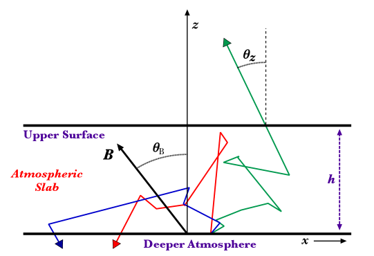
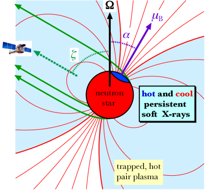
Figure 1: Left: Simulation geometry for transfer of photons through an atmospheric slab of height $\,h\,$ with a normal direction along the $\,z\,$ axis (zenith) and magnetic field, putatively in the $\,x-z\,$ plane, at an angle $\,\theta_{\hbox{\sixrm B}}\,$ to the local zenith. The green trajectory (projected on the $\,x-z\,$ plane) corresponds to a photon that scatters 10 times before exiting the top of the slab with zenith angle $\,\theta_{z}\,$, reaching the observer at infinity where its Stokes parameter information is recorded. The blue and red trajectories are for photons that scatter and eventually exit the bottom of the slab and are therefore unobservable. Adapted from Barchas, Hu & Baring (2021). Right: Global geometry of the spinning neutron star, displaying the inclination of the magnetic dipole moment $\,\hat{\bm{\mu}}_{\hbox{\fiverm B}}\,$ (purple, with dipolar field lines in curved spacetime displayed in red) to the rotation axis (signified using the angular velocity vector $\,\bm{\hat{\Omega}}\,$) by angle $\,\alpha\,$, and a particular viewing perspective (green arrow) for a telescope³ that is at an angle $\,\zeta\,$ to $\,\bm{\hat{\Omega}}\,$. Three coplanar curved trajectories (green) in the Schwarzschild metric are depicted for photons emanating towards the observer from different magnetic colatitudes on the stellar surface, with different local $\,\theta_{z}\,$ angles. The blue portion of the surface signifies a putatively hotter region and thereby identifies temperature non-uniformity of the stellar atmosphere.

2.2 Atmospheric Slab Injection Protocols

To render the simulation more accurate and efficient for moderate opacities, the anisotropy and polarization distributions of the photons injected at the base of the slab need to represent those appropriate for conditions deeper down in the atmosphere than MAGTHOMSCATT actually simulates. To achieve this, Barchas, Hu & Baring (2021) presented a high opacity photon simulation configuration, which captured the angular and the polarization information for photons fully processed by magnetic Thomson scatterings. This implementation described the asymptotic state of the scattering system regardless of photons’ spatial displacements or boundary conditions. The angular and polarization information merely depends on the photon frequency $\,\omega\,$ and the angle cosine $\,\mu=\cos\Theta_{\hbox{\sixrm kB}}\,$ of the photon wavevector $\,\bm{k}\,$ relative to $\,\hat{\bm{B}}\,$. This configuration is summarized using empirical approximations for the Stokes parameters:

$$I(\mu)\;=\;\hbox{${{\displaystyle A_{\omega}(\mu)\vphantom{(}}\over{\displaystyle\Lambda_{\omega}\,\sigma(\omega,\,\mu)\vphantom{(}}}$}\;\;,\quad A_{\omega}(\mu)\;=\;\hbox{${{\displaystyle 3\vphantom{(}}\over{\displaystyle 2\vphantom{(}}}$}\,\hbox{${{\displaystyle 1+{\cal A}(\omega)\,\mu^{2}\vphantom{(}}\over{\displaystyle 3+{\cal A}(\omega)\vphantom{(}}}$}\quad\hbox{for}\quad\mu\;=\;\hat{\bm{k}}\cdot\hat{\bm{B}}\;=\;\cos\Theta_{\hbox{\sixrm kB}}\quad,$$ (1)

where $\,I(\mu)\,$ is the anisotropic intensity of the asymptotic state, and

$$\hat{Q}_{\omega}(\mu)\;\equiv\;\hbox{${{\displaystyle Q\vphantom{(}}\over{\displaystyle I\vphantom{(}}}$}\;=\;\hbox{${{\displaystyle{\cal A}(\omega)\,\left[\mu^{2}-1\right]\vphantom{(}}\over{\displaystyle 1+{\cal A}(\omega)\,\mu^{2}\vphantom{(}}}$}\;\;,\quad\hat{V}_{\omega}(\mu)\;\equiv\;\hbox{${{\displaystyle V\vphantom{(}}\over{\displaystyle I\vphantom{(}}}$}\;=\;\hbox{${{\displaystyle 2{\cal C}(\omega)\,\mu\vphantom{(}}\over{\displaystyle 1+{\cal A}(\omega)\,\mu^{2}\vphantom{(}}}$}\quad,\quad\Pi_{\omega}\;=\;\sqrt{\bigl{(}\hat{Q}_{\omega}\bigr{)}^{2}+\bigl{(}\hat{V}_{\omega}\bigr{)}^{2}}$$ (2)

for the Stokes parameters that are normalized by the intensity $\,I(\mu)\,$, and the derivative total polarization degree $\,\Pi_{\omega}\,$. For local slab implementations, the coordinate basis used to establish the Stokes parameters can be chosen to render the Stokes $\,U\,$ to be zero; for more general geometries this no longer is possible: see Sec. 4.

The re-distribution anisotropy $\,A_{\omega}(\mu)\,$ constitutes the frequency-dependent asymptotic probability for re-distributing angles and polarizations through the scattering’s phase matrix (Chou, 1986). The intensity $\,I(\mu)\,$ satisfies traditional radiation transfer formalism on the sphere (e.g., Chandrasekhar, 1960), or equivalently a Boltzmann equation for the photon density distribution $\,n_{\gamma}(\mu)\propto I(\mu)/c\,$. It is therefore proportional to $\,A_{\omega}(\mu)\,$, yet is scaled by the relative probability for scattering, i.e. the total cross section $\,\sigma(\omega,\,\mu)\,$. We also introduce an additional normalization factor $\,\Lambda_{\omega}\,$ defined by

$$\Lambda_{\omega}\;=\;\int_{-1}^{1}\hbox{${{\displaystyle A_{\omega}(\mu)\vphantom{(}}\over{\displaystyle\sigma(\omega,\,\mu)\vphantom{(}}}$}\,d\mu\quad\Rightarrow\quad\int_{-1}^{1}I(\mu)\,d\mu\;=\;1\quad,$$ (3)

so that the intensity at the point of injection is normalized to unity for a photon. Note that this differs from the intensity normalization that is adopted for emergent photons in the graphical illustrations of Section 3, and also those realized in Section 5. The interpretations of $\,A_{\omega}(\mu)\,$, $\,\hat{Q}_{\omega}(\mu)\,$ and $\,\hat{V}_{\omega}(\mu)\,$, together with specific forms for the fitting functions for $\,{\cal A}(\omega)\,$ and $\,{\cal C}(\omega)\,$, are detailed in Sections 5.2 and 5.3 of Barchas, Hu & Baring (2021); we note here that both $\,{\cal A}\,$ and $\,\cal C\,$ are purely functions of the ratio $\,\omega/\omega_{\hbox{\fiverm B}}\,$, where $\,\omega_{\hbox{\fiverm B}}=eB/m_{e}c\,$ is the electron cyclotron frequency.

This asymptotic configuration applies to depths sufficiently remote from the upper slab surface. Thus, Barchas, Hu & Baring (2021) proposed that this choice defined an appropriate protocol for injecting photons at the base of the slab, closely approximating the true solution at moderate depths $\,h\,$ for a semi-infinite atmosphere. This expeditious approach is of particular importance in the strong field domain ($\,\omega/{\omega_{\hbox{\fiverm B}}}\ll 1\,$) where the total cross section for $\,\perp\,$ mode photons is significantly reduced relative to the non-magnetic Thomson value $\,\sigma_{\hbox{\fiverm T}}\,$. In this case, an extremely large $\,\tau_{\parallel}\,$ (see Eq. (6) below) is needed for the intensity and polarization angular profiles to saturate if one injects isotropic and unpolarized photons at the base, making for extremely large computation time. We therefore opt for the anisotropic and polarized injection in Eqs. (1) and (2) at the base of an atmospheric patch with arbitrary $\,\hat{\bm{B}}\,$ direction.

To specify the anisotropy, the direction of an injected photon is prescribed by applying the accept-reject method to the angular distribution of the flux $\,I(\mu)\cdot\cos\theta_{z0}\,$, using a random variate $\,\xi_{\mu}\,$, with $\,0<\xi_{\mu}<1\,$. Here, $\,\theta_{z0}\,$ is the angle of the photon wavevector to the slab normal, i.e., the zenith direction $\,\hat{z}\,$. Thus, $\,\cos\theta_{z0}=\hat{\bm{k}}\cdot\hat{z}\,$ and $\,I(\mu)\cdot\cos\theta_{z0}\,$ defines the photon flux of the intensity $\,I(\mu)\,$ passing through a surface element of unit area within the slab boundary. An alternative approach, not adopted here, is to select the direction of an injected photon using a two-step approach, first performing the accept-reject method for the intensity distribution $\,I(\mu)\,$, and then applying the flux weighting to the photon directions selected by the first step. We explored this possibility and compared these two selection protocols, determining that they give statistically equivalent results to a high degree of precision, as expected.

Next, the scaled Stokes parameters $\,\hat{Q}_{\omega}(\mu)\,$ and $\,\hat{V}_{\omega}(\mu)\,$ can be computed using Eq. (2), and the polarization state of the injected photon is determined by comparing the total polarization degree $\,\Pi_{\omega}\,$ with a random variable $\,\xi_{\Pi}\,$ in the range [0, 1]. If $\,\xi_{\Pi}\geq\Pi_{\omega}\,$, the photon is randomly chosen to be in the $\,\perp\,$ or $\,\parallel\,$ mode polarization states, generating a statistically unpolarized injection. These two orthogonal linear polarization modes in a magnetized medium are of common usage: the ordinary (O-mode) or $\,\parallel\,$ polarization state has an electric field vector $\,\bm{{\cal E}}\,$ in the plane defined by $\,\hat{\bm{k}}\,$ and $\,\hat{\bm{B}}\,$, with the extraordinary state (X-mode, denoted by $\,\perp\,$) having $\,\bm{{\cal E}}\,$ perpendicular to this plane. In terms of scaled Stokes parameters, both these polarizations have $\,\hat{V}=0\,$, with $\,\hat{Q}=-1\,$ for the $\,\perp\,$ state, and $\,\hat{Q}=+1\,$ for the $\,\parallel\,$ state. If instead $\,\xi_{\Pi}\leq\Pi_{\omega}\,$, the electric field components are specified by

$${\cal E}_{\theta}\;=\;\sqrt{\hbox{${{\displaystyle\Pi_{\omega}+\hat{Q}_{\omega}\vphantom{(}}\over{\displaystyle 2\Pi_{\omega}\vphantom{\bigl{(}}\vphantom{(}}}$}}\;,\quad{\cal E}_{\phi}\;=\;\hbox{${{\displaystyle i\hat{V}_{\omega}\vphantom{(}}\over{\displaystyle 2\Pi\,{\cal E}_{\theta}\vphantom{(}}}$}\;=\;i\,\hbox{sgn}(\hat{V}_{\omega})\,\sqrt{\hbox{${{\displaystyle\Pi_{\omega}-\hat{Q}_{\omega}\vphantom{(}}\over{\displaystyle 2\Pi_{\omega}\vphantom{\bigl{(}}\vphantom{(}}}$}}\;.$$ (4)

This defines a photon of elliptical polarization, for which the ratio of Stokes $\,Q\,$ and $\,V\,$ equals $\,\hat{Q}_{\omega}/\hat{V}_{\omega}\,$. In summary, employing just two random variates, $\,\xi_{\mu}\,$ and $\,\xi_{\Pi}\,$, the elliptically polarized photons and the statistically unpolarized $\,\perp/\parallel\,$ mode photons form a photon ensemble satisfying the asymptotic photon state described in Eqs. (1) and (2).

This anisotropic and polarized injection (AP) protocol establishes a fully scattered photon ensemble at the base of the atmospheric slab, circumventing the need to simulate the scatterings deep inside the atmospheres. Only photons emerging from the upper boundary are recorded, with their number $\,{\cal N}_{\rm rec}\,$ specified so as to generate the desired statistics as photons are sequentially injected. We performed tests using exploratory runs that excluded photons with small scattering numbers, to assess the role of the effective thickness of the slab. These tests revealed that such an exclusion is immaterial for most of the anisotropic and polarized injected simulations with modest optical depths, except for small $\,\omega/\omega_{\hbox{\fiverm B}}\,$ where the cross section strongly depends on the polarization and direction of the photon.

3 Polarization Characteristics from Localized Atmospheres

It is insightful to summarize the character of intensity and Stokes parameter information emerging from representative locales of atmospheric slabs at different magnetic colatitudes on neutron stars. This sets the scene for the varied contributions to the net signals from an extended region of the neutron star surface that propagate to an observer at infinity. This section presents an assemblage of such results by highlighting three particular locales, corresponding to magnetic colatitudes $\,\theta_{\hbox{\sixrm B}}=0^{\circ}\,$ (pole), $\,\theta_{\hbox{\sixrm B}}=45^{\circ}\,$ (mid latitudes) and $\,\theta_{\hbox{\sixrm B}}=90^{\circ}\,$ (equator). Furthermore, simulation results are presented for four select frequencies that bracket the cyclotron frequency, namely $\,\omega/\omega_{\hbox{\fiverm B}}=0.1,0.3,0.99,3\,$, spanning high-magnetic, sub-cyclotron domains and quasi-non-magnetic ones well above $\,\omega_{\hbox{\fiverm B}}\,$. These frequency and colatitude choices suffice to illustrate the intricate interplay between linear and circular polarizations.

For expediency, a compromise between precision and efficiency of atmospheric slab simulations must be achieved. High opacity runs yield greater precision, and low opacity runs are faster. Since opacity in magnetic environs is highly dependent on photon direction, we adopt a versatile measure of the effective optical depth $\,\tau_{\rm eff}\,$ in our simulations that captures the opacity and diffusion information at different frequencies and magnetic colatitudes. It is defined by

$$\tau_{{\hbox{\sixrm eff}}}\;=\;n_{e}h\,\sigma_{\rm up}(\theta_{i}\;=\;\theta_{\hbox{\sixrm B}})\;=\;\hbox{${{\displaystyle\tau_{\hbox{\fiverm T}}\vphantom{(}}\over{\displaystyle 2\vphantom{(}}}$}\Bigl{\{}\sin^{2}\theta_{\hbox{\sixrm B}}+\Sigma_{\hbox{\sixrm B}}(\omega)\left[1+\cos^{2}\theta_{\hbox{\sixrm B}}\right]\Bigr{\}}\;\;,\quad\hbox{for}\quad\Sigma_{\hbox{\sixrm B}}(\omega)\;=\;\hbox{${{\displaystyle\omega^{2}(\omega^{2}+\omega_{\hbox{\fiverm B}}^{2})\vphantom{(}}\over{\displaystyle(\omega^{2}-\omega_{\hbox{\fiverm B}}^{2})^{2}\vphantom{(}}}$}\quad.$$ (5)

This $\,\tau_{{\hbox{\sixrm eff}}}\,$ depth is calculated using the magnetic Thomson cross section $\,\sigma_{\rm up}\,$ for unpolarized (up) radiation (see Barchas, Hu & Baring (2021) for details) propagating along the local zenith, and therefore $\,\tau_{{\hbox{\sixrm eff}}}\,$ depends on the angle $\,\theta_{\hbox{\sixrm B}}\,$ and photon frequency $\,\omega\,$. In particular, two special cases, $\,\theta_{\hbox{\sixrm B}}=0^{\circ}\,$ and $\,90^{\circ}\,$, can be expressed via

$$\tau_{\parallel}\;=\;n_{e}h\,\sigma_{\rm up}(\theta_{i}=0^{\circ})\;=\;\tau_{\hbox{\fiverm T}}\,\Sigma_{\hbox{\sixrm B}}(\omega)\quad,\quad\tau_{\perp}\;=\;n_{e}h\,\sigma_{\rm up}(\theta_{i}=90^{\circ})\;=\;\hbox{${{\displaystyle\tau_{\hbox{\fiverm T}}\vphantom{(}}\over{\displaystyle 2\vphantom{(}}}$}\Bigl{[}1+\Sigma_{\hbox{\sixrm B}}(\omega)\Bigr{]}\quad.$$ (6)

These represent the optical depths at the magnetic pole and equator along the local zenith, and were employed in Barchas, Hu & Baring (2021). The effective optical depth defined in Eq. (5) satisfies $\,\tau_{{\hbox{\sixrm eff}}}\;=\;\tau_{\parallel}\cos^{2}\theta_{\hbox{\sixrm B}}+\tau_{\perp}\sin^{2}\theta_{\hbox{\sixrm B}}\,$, thereby representing a tensorial mix of diffusion properties parallel to and perpendicular to the magnetic field. For the purposes of efficiently developing representative results from atmospheric slabs at any surface locale, we will adopt $\,\tau_{{\hbox{\sixrm eff}}}=5\,$ in most of the runs for Fig. 2 and following. Yet we note that higher values of $\,\tau_{{\hbox{\sixrm eff}}}\,$ proved necessary at frequencies below the cyclotron resonance in order to accurately capture the polarization-dependence of the diffusion and generate accurate measures of Stokes parameters for radiation emerging from the slabs.

In the local slab simulations, for the purposes of illustration, intensity and polarization data for the photons escaping above the upper surface are collected in $\,n_{\theta}=90\,$ zenith angle bins and assigned a count number $\,{\cal N}_{j}\,$ in bin $\,j\,$. These angular bins are equally spaced on $\,[0,\pi/2]\,$ with a uniform width $\,\Delta\theta_{z}=\pi/(2n_{\theta})=1^{\circ}\,$, and they sum over all photon zenith azimuthal angles $\,\phi_{z}\,$. Note that this data accounting/binning choice differs from the protocol for the extended surface analysis of Section 5, described therein. The intensity for each $\,\theta_{z}\,$ bin is given by

$$I_{j}\;=\;\hbox{${{\displaystyle{\cal N}_{j}\vphantom{(}}\over{\displaystyle\cos\theta_{j}\sin\theta_{j}\,\Delta\theta_{z}\,{\cal N}_{\rm rec}\vphantom{(}}}$}\quad\Rightarrow\quad\sum_{j=1}^{n_{\theta}}I_{j}\cos\theta_{j}\sin\theta_{j}\,\Delta\theta_{z}\;=\;1\quad,$$ (7)

where the frequency dependence is not expressed explicitly, since most results in the paper are for mono-energetic photons. This can be easily adjusted for thermal spectra and cases of surface temperature non-uniformity, as desired. Note the total number $\,{\cal N}_{\rm rec}\,$ for recorded photons appears in the denominator, so that the intensity can be normalized to unity. Thus, intensities are weighted by the flux across the planar upper surface to the slab.

A suite of results for the three surface locales and four different (monochromatic) photon frequencies is presented in Fig. 2. For panels with $\,\omega/\omega_{\hbox{\fiverm B}}>0.3\,$, a depth of $\,\tau_{{\hbox{\sixrm eff}}}=5\,$ was adopted, collecting data from $\,10^{8}\,$ photons emergent through the top of the slab. For panels with $\,\omega/\omega_{\hbox{\fiverm B}}=0.3\,$ or $\,\omega/\omega_{\hbox{\fiverm B}}=0.1\,$, substantially higher $\,\tau_{{\hbox{\sixrm eff}}}\,$ values were chosen so that the simulations employing an anisotropic and polarized injection give the same results one would acquire with very large depths, namely $\,\tau_{{\hbox{\sixrm eff}}}>200\,$. This “asymptotic convergence” was tested to confirm that the results for polarized injection that are illustrated in Fig. 2 are robust. The intensity $\,I\,$, Stokes parameters $\,Q\,$, $\,V\,$ and total polarization degree $\,\Pi\,$ are integrated over the azimuthal angles about the local zenith and are plotted as functions of the zenith angle $\,\theta_{z}\,$. Accordingly, the intrinsic azimuthal dependence for non-polar slab locales is not explicitly illustrated. The Stokes $\,Q\,$, $\,V\,$ are normalized to the emergent intensity $\,I\,$. The intensity $\,I\,$ is normalized using Eq. (7), then multiplied by an extra factor of 0.5 in each panel to improve the visualization. For comparison, results from isotropic and unpolarized injection (IU) cases are displayed as traces with various markers for selected panels. This isotropic and unpolarized injection algorithm, a computationally less efficient choice, employs a statistically unpolarized and isotropic photon ensemble for the injection at the base of the slabs (see Section 3 of Barchas, Hu & Baring, 2021). We note that at large $\,\tau_{{\hbox{\sixrm eff}}}\gg 100\,$ the emergent Stokes parameter distributions are insensitive to the injection protocol.

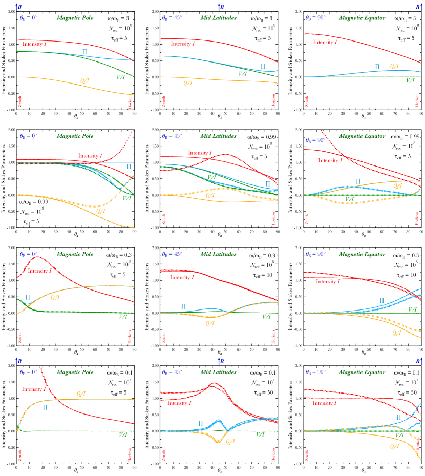
Figure 2: Angular distributions for intensity $\,I\,$ (red), Stokes parameters $\,Q/I\,$ (yellow-orange) and $\,V/I\,$ (green), and total polarization degree $\,\Pi\,$ (aqua) emergent from the top of the atmospheric slabs, as functions of zenith angle $\,\theta_{z}\,$ for slab runs at different locales, namely three magnetic colatitudes $\,\theta_{\hbox{\sixrm B}}=0^{\circ},45^{\circ}\,$ and $\,90^{\circ}\,$. The different rows display results for four different frequency ratios, $\,\omega/\omega_{\hbox{\fiverm B}}=3,0.99,0.3\,$ and $\,0.1\,$, from top to bottom. The optical depth is fixed at $\,\tau_{{\hbox{\sixrm eff}}}=5\,$ for $\,\omega/\omega_{\hbox{\fiverm B}}>0.3\,$. Solid histograms display the results for anisotropic and polarized injections, the preferred AP protocol. Also, traces with points (squares for $\,I\,$, vertical strokes for $\,Q/I\,$, dots for $\,V/I\,$ and crosses for $\,\Pi\,$) present results for isotropic and unpolarized injection, with all the photons emerging from the upper boundary being recorded (not displayed for all panels – see text for details).

For $\,\omega/\omega_{\hbox{\fiverm B}}=3\,$, the intensity profiles manifest slight anisotropy and they are insensitive to the emission locales and the injection methods. This approximates the “low-field” $\,\omega\gg\omega_{\hbox{\fiverm B}}\,$ domain where the magnetic field has limited impact on the scattering process and associated diffusion. The differential cross section then formally approaches the familiar non-magnetic one – see the Appendix of Barchas, Hu & Baring (2021) for a discussion. At the magnetic pole, the Stokes $\,V\,$ is strongest along the zenith direction, indicating significant circular polarization (+ mode) along $\,\bm{B}\,$, a direct consequence of the electron gyration captured in Eq. (18). The Stokes $\,Q\,$ that describes linear polarization is always negative and strongest along the horizon; this corresponds to a dominance of the $\,\perp\,$ mode, always possessing a larger cross section than the $\,\parallel\,$ mode ($\,\hat{Q}=+1\,$) when $\,\omega>\omega_{\hbox{\fiverm B}}\,$ – see Fig. B1 of Barchas, Hu & Baring (2021). The polarization signatures are considerably diminished at non-polar magnetic colatitudes $\,\theta_{\hbox{\sixrm B}}\,$ due to the integration over local azimuth: this convolution mixes the particular Stokes parameter information that is tied to the field direction and is summarized in Figs. 6 and 7 of Barchas, Hu & Baring (2021). In particular, the Stokes $\,V\,$ is always zero at the magnetic equator, a consequence of exact cancellation of $+$ and $-$ circular polarization contributions. Observe that the Stokes $\,Q\,$ parameter switches sign as the magnetic colatitude $\,\theta_{\hbox{\sixrm B}}\,$ increases in progressing from the pole to the equator, character that arises at all frequencies. This is a consequence of the Stokes parameters being calculated in a spherical coordinate system using the local zenith as a fixed reference direction. Misalignment of the magnetic field to the local zenith direction changes the Stokes $\,Q\,$ accordingly, but the dominance of $\,\perp\,$ mode polarization locally within the slab doesn’t change. The isotropic injection protocol gives very similar intensity and Stokes profiles at this frequency, and so they are not displayed in the Figure.

The second row of Fig. 2 presents results at $\,\omega/\omega_{\hbox{\fiverm B}}=0.99\,$, i.e., very near the cyclotron resonance. In this case, strong deviations appear between the distributions generated by the polarized and unpolarized injection protocols; this is expected because of the profound interplay between linear and circular polarizations in the scattering cross section. These disparities in emergent $\,I,Q,V\,$ and $\,\Pi\,$ profiles between polarized and unpolarized injection cases are strongest when the viewing perspectives are orthogonal to the magnetic field direction. This feature is best demonstrated at the magnetic pole, where the intensity histogram of the isotropic and unpolarized (IU) injection case realizes a fairly narrow peak at the horizon. The origin of these disparities is due to the cross section for $\,\parallel\,$ mode photons not being resonant when they are propagating orthogonal to $\,\bm{B}\,$. Therefore $\,\parallel\,$-polarized photons produced by the IU injection protocol can escape the atmosphere without scattering, thus contaminating the polarization signatures and forming an intensity peak perpendicular to the magnetic field direction. This feature disappears for the anisotropic, polarized injection protocol where scattering is more prolific on average. Test simulations have been performed for both injection protocols at $\,\omega/\omega_{\hbox{\fiverm B}}=0.99\,$ with higher optical depth. At the equator, for example, the convergence of the IU case doesn’t occur for $\,\tau_{{\hbox{\sixrm eff}}}<2000\,$, whereas the convergence of AP injection is clear at $\,\tau_{{\hbox{\sixrm eff}}}=5\,$, since $\,\tau_{{\hbox{\sixrm eff}}}=10,20\,$ runs result in statistically identical AP distributions. This fact highlights the advantage of the anisotropic and polarized injection protocol in more efficiently generating the correct Stokes parameter distributions emergent from the slab.

For the polarized injection case, the intensity profiles for $\,\omega/\omega_{\hbox{\fiverm B}}=0.99\,$ don’t change much from their $\,\omega/\omega_{\hbox{\fiverm B}}=3\,$ counterparts. In contrast, the polarization information does change with this lowering of frequency, somewhat for $\,V\,$ and more so for $\,Q\,$. The predominance of the $\,\perp\,$ mode photons ($\,Q<0\,$) is now more marked and so the net polarization degree $\,\Pi\,$ is enhanced, approaching 100 per cent at the magnetic pole, regardless of the zenith angle. This is a key signature of the polarizing influence of driven electron gyration. For this polar case, the directional trade-off between circular and linear polarizations is obvious. For the equatorial example, Stokes $\,V\,$ is again always zero due to the cancellations incurred with azimuthal integration. As with the $\,\omega/\omega_{\hbox{\fiverm B}}=3\,$ case, only a modest $\,\tau_{{\hbox{\sixrm eff}}}=5\,$ is required at resonance for the anisotropic, polarized injection to precisely yield the asymptotic, thick slab signals.

The intensity and Stokes parameter distributions change noticeably when the frequency drops below the “equipartition frequency” $\,\omega/\omega_{\hbox{\fiverm B}}=1/\sqrt{3}\approx 0.577\,$, where linear polarization cross sections are identical to the Thomson value $\,\sigma_{\hbox{\fiverm T}}\,$: see Barchas, Hu & Baring (2021). This $\,\omega\ll\omega_{\hbox{\fiverm B}}\,$ domain is where the field strongly impacts the scattering process. The intensity is beamed close to the $\,\bm{B}\,$ direction, since the cross section is strongly reduced, i.e. $\,\sigma\sim\sigma_{\hbox{\fiverm T}}(\omega/\omega_{\hbox{\fiverm B}})^{2}\,$, for photons propagating along the magnetic field lines, regardless of their polarization. This beaming effect is significant at the magnetic pole and realizes a peak at $\,\theta_{b}\sim\omega/\omega_{\hbox{\fiverm B}}\,$. The angular dependence of the peak beaming angle $\,\theta_{b}\,$ is associated with the transition from $\,\perp\,$ to $\,\parallel\,$ mode polarization close to the magnetic field, reflecting the interplay between frequency and angular dependence in the differential cross sections (see Appendix B of Barchas, Hu & Baring, 2021). For $\,\omega/\omega_{\hbox{\fiverm B}}=0.3\,$, the intensity beaming is muted due to azimuth integration and flux weighting at emission locales other than the magnetic pole. Yet, for lower frequencies like $\,\omega/\omega_{\hbox{\fiverm B}}=0.1\,$, the beaming effect is so strong that it cannot be completely eliminated by azimuth integration, leaving an intensity enhancement at $\,\theta_{z}\sim 45^{\circ}\,$ for the mid-latitude case. The $\,\parallel\,$ mode dominates the emergent radiation, while the circular portion is very weak unless viewing along the $\,\bm{B}\,$ direction. Note that we increase the $\,\tau_{{\hbox{\sixrm eff}}}\,$ for the non-polar cases with $\,\omega/\omega_{\hbox{\fiverm B}}\leq 0.3\,$ in order to realize the asymptotic results expected for very thick slabs. Then, photon diffusion is strong along the magnetic field at $\,\omega\ll\omega_{\hbox{\fiverm B}}\,$, while the parameterization of $\,\tau_{{\hbox{\sixrm eff}}}\,$ only captures photon diffusion along the local zenith. Test runs revealed that increasing $\,\tau_{{\hbox{\sixrm eff}}}\,$ above those chosen for the AP runs displayed in all panels in Fig. 2 did not incur appreciable changes to any of the $\,I\,$, $\,Q\,$, $\,V\,$ and $\,\Pi\,$ distributions. As with the resonant frequency case, for $\,\omega/\omega_{\hbox{\fiverm B}}=0.1\,$ the IU run results displayed have not realized such convergence to the AP distributions, requiring much larger values of $\,\tau_{{\hbox{\sixrm eff}}}\,$ to achieve this asymptotically thick slab state.

4 Stokes Parameter Transmission in General Relativity

This section focuses on the general relativistic (GR) framework for the parallel transport of the polarization information of light through the magnetosphere in the curved spacetime of the non-rotating Schwarzschild metric. This choice of metric is widely applicable to various classes of neutron stars that emit X rays, perhaps with the exception of millisecond pulsars, and the principal influences can be identified without imbuing the analysis with the complexities of rotating metrics. Since the magnetic field structure and ray tracing of light in Schwarzschild spacetime are well-known, the details of them as implemented in MAGTHOMSCATT are summarized in Appendix B, therein also detailing our testing protocols for the GR ray tracing.

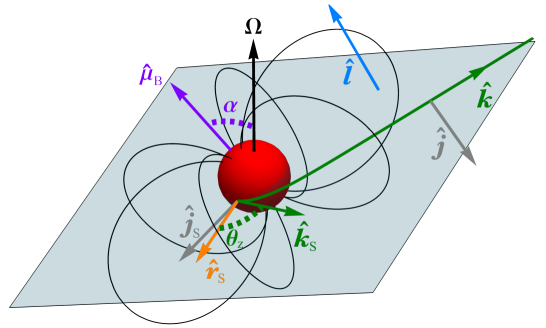
Figure 3: Global geometry of a spinning neutron star with a inclination angle $\,\alpha\,$ between the angular velocity vector $\,\bm{\hat{\Omega}}\,$ and the magnetic dipole moment $\,\hat{\bm{\mu}}_{\hbox{\fiverm B}}\,$. The trajectory plane (light blue) is decided by the cross product of the emission locale vector $\,\hat{\bm{r}}_{\hbox{\fiverm S}}\,$ and the wavevector $\,\hat{\bm{k}}_{\hbox{\fiverm S}}\,$, and it contains the $\,\hat{\bm{j}}_{\hbox{\fiverm S}}\,$, $\,\hat{\bm{k}}_{\hbox{\fiverm S}}\,$, $\,\hat{\bm{j}}\,$ and $\,\hat{\bm{k}}\,$ vectors (see text). The angular momentum vector $\,\hat{\bm{l}}\,$ (blue) of the photon trajectory is a constant of motion and is perpendicular to the trajectory plane.

4.1 Polarization: Parallel Transport – Mapping Surface to Observer

In the absence of plasma dispersion and vacuum birefringence, the propagation of electromagnetic waves outside a neutron star can be well described by the geometric optics approximation. The polarization 4-vector $\,{\cal E}^{\mu}\,$ of the vector potential undergoes parallel transport along the null geodesic of a light ray and is always perpendicular to the 4-wavevector $\,k^{\mu}\,$ (e.g., see Section 22.5 of Misner et al., 1973). In a given frame, the time component of $\,{\cal E}^{\mu}\,$ doesn’t affect the measured electric and magnetic fields, so it is normally set to zero for simplicity. The polarization 3-vector (electric field) $\,\bm{{\cal E}}\,$ lies in the polarization plane perpendicular to the 3-wavevector $\,\bm{k}\,$. Throughout the propagation, $\,\bm{{\cal E}}\,$ keeps a fixed angle along its trajectory with respect to the photon orbital angular momentum unit vector $\,\hat{\bm{l}}\,$ through the sequence of local inertial frames from the surface to infinity (Pineault, 1977). This property simplifies the parallel transport of the polarization vector $\,\bm{{\cal E}}\,$ as the $\,\bm{{\cal E}}-\hat{\bm{l}}\,$ plane rotates and remains perpendicular to $\,\bm{k}\,$, with the components of $\,\bm{{\cal E}}\,$ in the LIF parallel to and perpendicular to the trajectory plane being constants of the motion. Implementations of this picture can be found in Pavlov & Zavlin (2000) and Heyl et al. (2003).

To specify the polarization at the stellar surface and infinity, we define two groups of orthogonal basis vectors $\,\{\hat{\bm{j}}_{\hbox{\fiverm S}},\hat{\bm{k}}_{\hbox{\fiverm S}},\hat{\bm{l}}\}\,$ and $\,\{\hat{\bm{j}}_{{\fiverm{\infty}}},\hat{\bm{k}}_{{\fiverm{\infty}}},\hat{\bm{l}}\}\,$ for a photon at the emission (surface) and observer locales respectively:

$$\hat{\bm{l}}\;=\;\hbox{${{\displaystyle\hat{\bm{r}}_{i}\times\hat{\bm{k}}_{i}\vphantom{(}}\over{\displaystyle|\hat{\bm{r}}_{i}\times\hat{\bm{k}}_{i}|\vphantom{(}}}$}\quad\text{and}\quad\hat{\bm{j}}_{i}=\hat{\bm{k}}_{i}\times\hat{\bm{l}}\quad,$$ (8)

where $\,i=S\,$ or $\,\infty\,$, denoting the stellar surface and the observer at infinity. The vector $\,\hat{\bm{k}}_{i}\,$ is the unit 3-wavevector and $\,\hat{\bm{r}}_{i}\,$ is the unit displacement vector of the photon with respect to the center of the star, with them generating $\,\hat{\bm{l}}\,$, the constant unit orbital angular momentum vector. The $\,\hat{\bm{j}}_{i}\,$ vector always lies in the polarization plane. The differential in the polarization vector though parallel transport from one LIF to another is mediated by the affine connection according to $\,d{\cal E}^{\mu}=-\Gamma^{\mu}_{\nu\lambda}dx^{\lambda}\,{\cal E}^{\nu}\,$ (e.g., see Sec. 4.9 of Weinberg, 1972). The cumulative increment of this differential along the trajectory is described simply by a rotation through a single angle, $\,\eta_{\hbox{\fiverm S}}-\theta_{z}\,$, representing the bending angle of the photon momentum vector from surface to infinity; this is summarized in Pineault (1977). Here, $\,\eta_{\hbox{\fiverm S}}\,$ defines the angle around the stellar surface in its LIF from the photon emission point $\,\bm{r}_{\hbox{\fiverm S}}\,$ to the point $\,R_{\hbox{\sixrm NS}}\hat{\bm{r}}_{\infty}\,$ on the surface radially in the direction to the observer. Since the photon emerges from the atmosphere in the direction $\,\hat{\bm{k}}_{\hbox{\fiverm S}}=\bm{k}_{\hbox{\fiverm GR}}(\Psi=\Psi_{\hbox{\sixrm S}})/|\bm{k}_{\hbox{\fiverm GR}}|\,$ at an angle $\,\theta_{z}\,$ to its local zenith, its $\,\hat{\bm{j}}_{\hbox{\fiverm S}}-\hat{\bm{l}}\,$ plane of polarization lies at an angle $\,\eta_{\hbox{\fiverm S}}-\theta_{z}\,$ to the plane normal to $\,R_{\hbox{\sixrm NS}}\hat{\bm{r}}_{\infty}\,$ in the LIF at the surface. Simple geometry on the sphere relates the various unit vectors:

$$\hat{\bm{j}}_{{\fiverm{\infty}}}\;=\;\sin{(\eta_{\hbox{\fiverm S}}-\theta_{z})}\hat{\bm{k}}_{\hbox{\fiverm S}}+\cos(\eta_{\hbox{\fiverm S}}-\theta_{z})\hat{\bm{j}}_{\hbox{\fiverm S}}\quad\text{and}\quad\hat{\bm{k}}_{{\fiverm{\infty}}}\;=\;\cos{(\eta_{\hbox{\fiverm S}}-\theta_{z})}\hat{\bm{k}}_{\hbox{\fiverm S}}-\sin(\eta_{\hbox{\fiverm S}}-\theta_{z})\hat{\bm{j}}_{\hbox{\fiverm S}}\quad.$$ (9)

It is convenient to resolve the polarization vector $\,\hat{\bm{{\cal E}}}_{\hbox{\fiverm S}}\,$ in terms of components parallel to $\,\hat{\bm{l}}\,$ and $\,\hat{\bm{j}}_{\hbox{\fiverm S}}\,$ at the stellar surface: $\,\hat{\bm{{\cal E}}}_{\hbox{\fiverm S}}={\cal{E}}_{l}\hat{\bm{l}}+{\cal{E}}_{j}\hat{\bm{j}}_{\hbox{\fiverm S}}\,$. The components of $\,\hat{\bm{{\cal E}}}_{\hbox{\fiverm S}}\,$ projected onto the $\,\hat{\bm{j}}_{{\fiverm{\infty}}}-\hat{\bm{l}}\,$ plane are then $\,{\cal{E}}_{l}\hat{\bm{l}}\,$ and $\,{\cal{E}}_{j}\hat{\bm{j}}_{{\fiverm{\infty}}}\,$. One quickly concludes that the polarization vector measured by an observer at infinity is then simply

$$\hat{\bm{{\cal E}}}_{{\fiverm{\infty}}}\;=\;{\cal{E}}_{l}\hat{\bm{l}}+{\cal{E}}_{j}\hat{\bm{j}}_{{\fiverm{\infty}}}\;\;,\quad\hbox{with}\quad{\cal{E}}_{l}\;=\;\hat{\bm{{\cal E}}}_{\hbox{\fiverm S}}\cdot\hat{\bm{l}}\quad,\quad{\cal{E}}_{j}\;=\;\hat{\bm{{\cal E}}}_{\hbox{\fiverm S}}\cdot\hat{\bm{j}}_{\hbox{\fiverm S}}\quad,$$ (10)

with Eq. (9) capturing the rotation information. The protocols we employed for testing the polarization transport implementation are discussed in Appendix C.

Polarization is conveniently measured at infinity, for any rotational phase, using Cartesian coordinate basis vectors defined with respect to the plane defined by $\,\hat{\bm{k}}_{{\fiverm{\infty}}}\,$ and the stellar angular momentum vector $\,\bm{\hat{\Omega}}\,$ of the star, i.e.,

$$\hat{y}\;=\;\hbox{${{\displaystyle\bm{\hat{\Omega}}\times\hat{\bm{k}}_{\infty}\vphantom{(}}\over{\displaystyle|\bm{\hat{\Omega}}\times\hat{\bm{k}}_{\infty}|\vphantom{(}}}$}\quad\text{and}\quad\hat{x}\;=\;\hat{y}\times\hat{\bm{k}}_{\infty}\quad,$$ (11)

so that obviously $\,\hat{\bm{k}}_{\infty}=\hat{z}\,$. For $\,\cos\zeta=\hat{\bm{k}}_{\infty}\cdot\bm{\hat{\Omega}}\,$, one then deduces that $\,\bm{\hat{\Omega}}=-\sin\zeta\,\hat{x}+\cos\zeta\,\hat{z}\,$. The corresponding components of the electric field vector are then $\,{\cal{E}}_{x}=\hat{\bm{{\cal E}}}_{{\fiverm{\infty}}}\cdot\hat{x}\,$ and $\,{\cal{E}}_{y}=\hat{\bm{{\cal E}}}_{{\fiverm{\infty}}}\cdot\hat{y}\,$, and these can be inserted in Eq. (21) to compute the Stokes parameters. The photon electric field component parallel to the $\,\hat{x}\,$ contributes to a positive $\,Q\,$ value while the component parallel to the $\,\hat{y}\,$ contributes to a negative $\,Q\,$.

4.2 Observables for rotating neutron stars

In detailing how the photon momentum and polarization vectors are transported from the stellar surface to infinity, the spin axis $\,\bm{\hat{\Omega}}\,$ and the observer’s direction $\,\hat{\bm{k}}_{{\fiverm{\infty}}}\,$ are fixed. Yet this propagation is independent of the magnetic moment orientation $\,\hat{\bm{\mu}}_{\hbox{\fiverm B}}\,$ which rotates as the star spins. The zero of phase $\,\Omega t=0\,$ is chosen to be when the magnetic axis $\,\hat{\bm{\mu}}_{\hbox{\fiverm B}}\,$ is coplanar with $\,\bm{\hat{\Omega}}\,$ and $\,\hat{\bm{k}}_{{\fiverm{\infty}}}\,$. The vector $\,\hat{\bm{k}}_{{\fiverm{\infty}}}\,$, characterized by a viewing angle $\,\zeta\,$ such that $\,\cos\zeta=\bm{\hat{\Omega}}\cdot\hat{\bm{k}}_{{\fiverm{\infty}}}\,$, corresponds to an infinite number of trajectories directed to a specific observer. For a given $\,\eta_{\hbox{\fiverm S}}\,$, these trajectories form a cylinder at infinity that is constricted down near the surface where the intersection of this trajectory surface with the star is a circle. This circle samples a variety of magnetic colatitudes and longitudes, values that are modulated as the star rotates. The instantaneous viewing angle $\,\theta_{v}\,$ between the line of sight, $\,\hat{\bm{k}}_{{\fiverm{\infty}}}\,$, and the magnetic axis, $\,\hat{\bm{\mu}}_{\hbox{\fiverm B}}\,$, can be expressed in relation to $\,\bm{\hat{\Omega}}\,$ via a spherical triangle relation (see section 4.3 of Hu et al., 2019):

$$\cos\theta_{v}\;\equiv\;\hat{\bm{k}}_{{\fiverm{\infty}}}\cdot\hat{\bm{\mu}}_{\hbox{\fiverm B}}\;=\;\cos\alpha\cos\zeta+\sin\alpha\sin\zeta\cos\Phi\quad,$$ (12)

where $\,\alpha\,$ is the inclination angle, $\,\zeta\,$ is the observer angle and $\,\Phi=\Omega t\,$ is the rotation phase. This relation controls how the atmospheric emission information at a given surface locale maps to observers at all rotational phases. When a photon escapes the atmosphere at a certain locale, its local $\,\hat{\bm{{\cal E}}}_{\hbox{\fiverm S}}\,$, $\,\hat{\bm{k}}_{\hbox{\fiverm S}}\,$, $\,\hat{\bm{l}}\,$ and $\,\hat{\bm{j}}_{\hbox{\fiverm S}}\,$ vectors are specified in Cartesian form. In order to treat a star with arbitrary inclination angle and rotational phase, we rotate the star and all these vectors first through $\,\alpha\,$ from the local magnetic coordinate description identified in Appendix B, and then through the phase $\,\Phi=\Omega t\,$. The rotated vectors at the surface are then transported to infinity using Eqs. (9) and (10).

In the simulation, we collect all the photons that propagate to infinity after they emerge from the neutron star atmospheric locale where their radiative transport is computed. This is equivalent to having a large number of observers spanning the entire sky. Information captured by observers with the same $\,\zeta\,$ but different azimuth angles $\,\Phi\,$ about the spin axis $\,\bm{\hat{\Omega}}\,$ essentially corresponds to the information collected by the same observer of different rotational phases $\,\Phi\to-\Omega t\,$. In this way, we circumvent the need to simulate different rotational configurations and are able to collect information of all the rotational phases from a single simulation run, subsequently assigning it to a rotational phase for each binned value of $\,\zeta\,$. This is the protocol we adopt for the sky maps illustrated in Sec. 5.

5 Polarization Characteristics from Extended Atmospheres

In this Section, the ensemble intensity and polarization signals are computed for extended surface regions. For each injected photon, the emitting locale is uniformly sampled from the prescribed surface region, which for simplicity is chosen to be a spherical rectangular patch bounded by fixed magnetic colatitudes $\,\theta\,$ and longitudes $\,\phi\,$ defined by the GR dipole construction detailed in Appendix B. Throughout the paper, $\,M=1.44M_{\odot}\,$ and $\,R_{\hbox{\sixrm NS}}=10^{6}\,$ cm are adopted. Emission locales inside the spherical rectangle patch are sampled using

$$\cos\theta\;=\;\cos{\theta_{l}}+(\cos{\theta_{u}}-\cos{\theta_{l}})*\xi_{\theta}\quad\text{and}\quad\phi\;=\;\phi_{l}+(\phi_{u}-\phi_{l})*\xi_{\phi}\quad,$$ (13)

where $\,\theta_{l},\theta_{u},\phi_{l}\,$, and $\,\phi_{u}\,$ are the boundary coordinates of the patch, and $\,\xi_{\theta}\,$ and $\,\xi_{\phi}\,$ are random variates. This sampling is therefore uniform in solid angle within the spherical rectangle, and is routinely adaptable to treat temperature gradients that are inferred for most neutron star systems. Throughout, azimuthal symmetry is presumed, corresponding to $\,\phi_{l}=0\,$ and $\,\phi_{u}=2\pi\,$. For each photon, the local atmospheric transport simulation was performed as described in Sec. 3 and then propagated to infinity as detailed in Sec. 4, recording its direction in the sky and its Stokes parameters.

5.1 Entire Surface

The intensity $\,I\,$, Stokes parameters $\,Q/I,U/I\,$ and $\,V/I\,$ from a uniformly emitting star, where 5$\,\times 10^{9}\,$ photons are recorded for atmospheric slab simulations distributed randomly across the whole surface, are illustrated as sky maps in Figure. 4. The coordinates in these maps are the rotational phase $\,\Phi=\Omega t\,$ on the x-axis and the observer’s viewing angle $\,\zeta\,$ relative to the spin axis on the y-axis. Accordingly, the maps are akin to those used in models of gamma-ray pulsars (Harding & Kalapotharakos, 2015, 2017). The mass of the star is fixed at $\,1.44M_{\odot}\,$ which corresponds to a surface radial parameter $\,\Psi_{\hbox{\sixrm S}}\approx 0.425\,$. For each panel, the photon frequency $\,\omega\,$ is fixed so that $\,\omega/\omega_{\hbox{\fiverm B}}=0.1\,$ in the LIF at the magnetic poles, with a corresponding value of $\,\omega/\omega_{\hbox{\fiverm B}}=0.175\,$ at the magnetic equator. From left to right, each column in Figure. 4 displays results for inclination angles $\,\alpha=15^{\circ},45^{\circ}\,$ and $\,75^{\circ}\,$. The sky maps are binned with both $\,\zeta\,$ and $\,\Phi\,$ resolutions of $\,3^{\circ}\,$, hence the average photon count per pixel is around $\,3\times 10^{4}\,$.

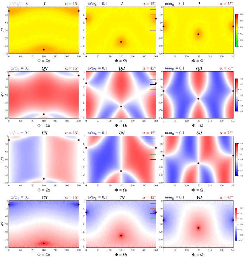
Figure 4: Intensity and polarization sky map distributions obtained via general relativistic propagation of simulated atmospheric signals from a uniformly emitting star. The sky distributions are plotted as functions of the viewing angle $\,\zeta\,$ and rotation phase $\,\Phi=\Omega t\,$, with scales indicated in the color legend bars at the right of each row. The inclination angle of the star $\,\alpha\,$ is set to $\,15^{\circ},45^{\circ}\,$ and $\,75^{\circ}\,$ for the columns from left to right, and the mass is $\,1.44M_{\odot}\,$($\,\Psi_{\hbox{\sixrm S}}\approx 0.425\,$). The frequency of the emitted photons is fixed with a ratio $\,\omega/\omega_{\hbox{\fiverm B}}=0.1\,$ in the LIF at the magnetic poles, and is higher at all other colatitudes where the surface field is lower. The number of the recorded photons is $\,{\cal N}_{\rm rec}=5\times 10^{9}\,$ for each panel. The black dots in each panel mark the $\,(\zeta,\,\Phi)\,$ combinations for which the observer is instantaneously viewing along the magnetic axis $\,\hat{\bm{\mu}}_{\hbox{\fiverm B}}\,$. In the $\,\alpha=45^{\circ}\,$ panels, horizontal lines mark the $\,\zeta\,$ values used to assemble the pulse profiles displayed in Fig. 6 with the same color coding.

The intensity maps display moderate anisotropy with an average value equalling $\,1/(4\pi)\sim 0.08\,$, the intensity normalization. The intensity is maximized when the observer’s line of sight is parallel or antiparallel to the magnetic axis $\,\hat{\bm{\mu}}_{\hbox{\fiverm B}}\,$. These viewing directions are marked by circled dots in all the sky maps. The maximum intensity is only around 6% greater than the average value. The maxima are due to both the local beaming of radiation emerging from the surface and the GR lensing of light. The local beaming of the emitted photons is controlled by the local field direction and strength in the atmosphere: see Fig. 2 for examples. Yet, since a specific observer detects photons from regions encapsulating a range of field strengths and widely differing directions, the intensity variations evident in from the array in Fig. 2 are moderated considerably. In addition, the GR light bending effect increases the visible surface of the star (e.g. see Nollert et al., 1989) by 74% for our choice of $\,M\,$ and $\,R_{\hbox{\sixrm NS}}\,$, providing access to the far side of the star, so that the intensity variations are further changed. When $\,M\to 0\,$ (i.e., $\,\Psi_{\hbox{\sixrm S}}=0\,$) and the GR influences are removed, the intensity variation is enhanced to around 30%, with maxima for viewing directions roughly perpendicular to $\,\hat{\bm{\mu}}_{\hbox{\fiverm B}}\,$, i.e., over equatorial regions of larger surface area.

The $\,Q/I\,$ and $\,U/I\,$ maps are displayed in the second and the third row of Fig. 4 respectively. Here the Stokes parameters are measured using axes defined in Eq. (11), i.e., with respect to the plane defined by the observer direction $\,\hat{\bm{k}}_{{\fiverm{\infty}}}\,$ and the stellar rotational vector $\,\bm{\hat{\Omega}}\,$. This coordinate choice differs from that adopted for the panels in Fig. 2 where Stokes parameters are measured with respect to the plane defined by the photon emission direction and the normal to the atmospheric slab (zenith). The Stokes $\,Q/I\,$ is mainly positive for stars with small $\,\alpha\,$. This is because the $\,\parallel\,$ mode polarization dominates the outgoing emission at the selected frequency range, and the projection of the magnetic axis on the observer’s sky is almost parallel to the reference axis $\,\hat{x}\,$ defined in Eq. (11) for small $\,\alpha\,$. As the inclination angle $\,\alpha\,$ increases, the $\,Q/I\,$ sky map pattern is noticeably more complicated, and the $\,Q/I\,$ values become sensitive to $\,\zeta\,$ and $\,\Phi\,$. This modulation arises because the projection of the magnetic axis on the sky oscillates around the $\,\hat{x}\,$ axis as the star rotates. The $\,U/I\,$ values are generally non-zero unless the projection of the magnetic axis on the observer’s sky is parallel or antiparallel to one of the reference axes ($\,\hat{x},\hat{y}\,$) for the Stokes parameters. The typical linear polarization degree is around 0.2, which is slightly higher than the flat spacetime values in Fig. 5.5 of Barchas (2017). The $\,V/I\,$ results are shown in the last row. The typical $\,V/I\,$ value is around 0.02, which is much smaller than the typical linear polarization degree. The right-handed and left-handed photons dominate the circular polarization when the observer is instantaneously looking down the south or the north magnetic pole. The value and the sign of the $\,V/I\,$ reflect the convolution of a wide variety of magnetic field directions on the stellar surface, and is naturally expected to be small. Due to the hemispherical and the azimuthal symmetries of the dipole configuration that is uniformly sampled by photons, the Stokes parameters in all the maps satisfy the following relations:

$$I(\zeta,\Phi)\;=\;I(180^{\circ}-\zeta,180^{\circ}-\Phi) \;=\; I(180^{\circ}-\zeta,180^{\circ}+\Phi)\;=\;I(\zeta,360^{\circ}-\Phi),$$

$$\hat{Q}(\zeta,\Phi)\;=\;\hat{Q}(180^{\circ}-\zeta,180^{\circ}-\Phi) = \hat{Q}(180^{\circ}-\zeta,180^{\circ}+\Phi)\;=\;\hat{Q}(\zeta,360^{\circ}-\Phi),$$

$$\hat{U}(\zeta,\Phi)\;=\;\hat{U}(180^{\circ}-\zeta,180^{\circ}-\Phi) = -\hat{U}(180^{\circ}-\zeta,180^{\circ}+\Phi)\;=\;-\hat{U}(\zeta,360^{\circ}-\Phi),$$

$$\hat{V}(\zeta,\Phi)\;=\;-\hat{V}(180^{\circ}-\zeta,180^{\circ}-\Phi) = -\hat{V}(180^{\circ}-\zeta,180^{\circ}+\Phi)\;=\;\hat{V}(\zeta,360^{\circ}-\Phi).$$

Note that a minus sign appears in the $\,V/I\,$ relation, being related to the direction of the magnetic field. The linear polarization present here, with typical degrees of $\,\Pi_{l}\sim 20\,$%, should be detectable by IXPE (Weisskopf et al., 2016) in sources providing sufficient photon count statistics, for example select magnetars. The vacuum birefringence effects of polarization transport in the magnetized quantum vacuum will largely preserve the polarization of photons when they propagate through the magnetosphere (Heyl et al., 2003); their treatment is deferred to future investigations.

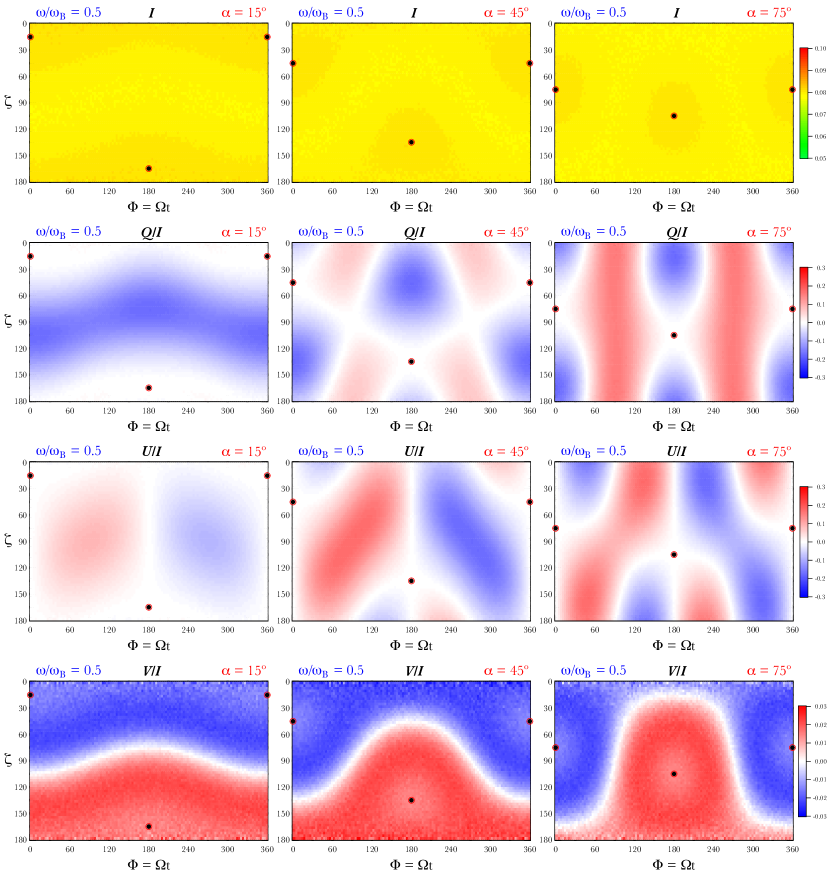
Figure 5: Same as for Fig. 4, but with a photon frequency ratio $\,\omega/\omega_{\hbox{\fiverm B}}=0.5\,$ at the magnetic poles. The intensity modulations are more limited and the degree of polarization is reduced slightly relative to Fig. 4. Observe that the signs of $\,Q/I\,$ and $\,U/I\,$ are generally the opposite of those for the $\,\omega/\omega_{\hbox{\fiverm B}}=0.1\,$ case due to the character of the scattering cross section (see text).

Fig. 5 presents the results for frequency ratio $\,\omega/\omega_{\hbox{\fiverm B}}=0.5\,$ in the LIF at the magnetic poles, chosen to closely represent the surface X-ray emission from a moderately magnetized neutron star. In this case, the intensity and Stokes parameter maps share very similar $\,\Phi-\zeta\,$ patterns to those in Fig. 4. Yet the intensity at each surface atmospheric locale in this case is more isotropic than that for the lower $\,\omega/\omega_{\hbox{\fiverm B}}\,$, with the maximum intensity only around 1% greater than the average value. This is because the photon cross section in the $\,0.5<\omega/\omega_{\hbox{\fiverm B}}<0.9\,$ range is less sensitive to the polarization states and scattering angles. Therefore the local intensity beaming is relatively muted, as can be seen from Fig. 2. The result is that the very low pulse fraction does not match those typically observed in isolated X-ray pulsars, indicating that the region of their dominant emission is probably far inferior to the entire surface. Alternatively, or in addition, the observed high pulse fraction could be caused by the intrinsic beaming of the radiation emergent from atmospheres in select surface locales. The linear polarization degree is weaker than that in Fig. 4, with a typical value around 0.1. In this case the Stokes $\,Q/I\,$ is mainly negative for small $\,\alpha\,$, as opposed to the $\,\omega/\omega_{\hbox{\fiverm B}}=0.1\,$ case, where it is then mostly positive. This difference reflects the transition of the dominant linear polarization mode from $\,\parallel\,$ to $\,\perp\,$ when $\,\omega/\omega_{\hbox{\fiverm B}}\,$ crosses the critical value $\,1/\sqrt{3}\sim 0.577\,$: see Eq. (5), Fig. 2 or Barchas, Hu & Baring (2021) for a detailed discussion of this nuance pertaining to the scattering cross section. The Stokes $\,U/I\,$ also experiences this general switch of sign for the $\,\omega/\omega_{\hbox{\fiverm B}}=0.5\,$ case relative to the $\,\omega/\omega_{\hbox{\fiverm B}}=0.1\,$ one. The circular polarization is similar to that in Fig. 4 with a typical circular polarization degree around $\,0.02\,$, much smaller than the linear polarization degree. Again, this is the result of directional mixing of the fields even for viewing angles above the magnetic poles.

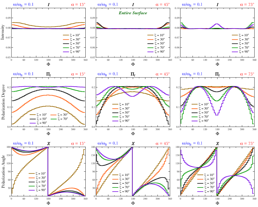
Figure 6: Simulated pulse profiles for a uniformly emitting entire stellar surface, for intensity $\,I\,$, linear polarization degree $\,\Pi_{l}\,$ and polarization angle $\,\chi\,$, top to bottom, plotted as functions of the rotation phase $\,\Phi\,$ for selected viewing angles $\,\zeta=10^{\circ},30^{\circ},50^{\circ},70^{\circ}\,$ and $\,90^{\circ}\,$. These pulse profiles correspond to the horizontal cuts of the sky map panels in Fig. 4, signified in the $\,\alpha=45^{\circ}\,$ panels by the horizontal bars that are color coded to match the profiles displayed here. Each column displays results for one of the three selected magnetic inclination angles $\,\alpha=15^{\circ},45^{\circ},75^{\circ}\,$, and the frequency of the photons is fixed so that $\,\omega/\omega_{\hbox{\fiverm B}}=0.1\,$ at the magnetic poles in the LIF, i.e. $\,\omega/\omega_{\hbox{\fiverm B}}=0.175\,$ at the equator.

To connect to observables pertinent to X-ray telescopes, the pulse profiles for intensity $\,I\,$, linear polarization degree $\,\Pi_{l}=\sqrt{Q^{2}+U^{2}}/I\,$ and polarization angle $\,\chi=[\arctan{(U/Q)}]/2\,$ are presented in Fig. 6 for $\,\omega/\omega_{\hbox{\fiverm B}}=0.1\,$ and selected observing angles. Pulse profiles for the $\,\omega/\omega_{\hbox{\fiverm B}}=0.5\,$ case are morphologically similar, and so are not explicitly displayed in the interest of brevity. The profiles displayed in Fig. 6 are derived from horizontal sections of Fig. 4, and are averaged using the symmetries in Eq. (LABEL:eq:IQUV_sym) so as to decrease statistical fluctuations. The selected observing angles are indicated as horizontal cuts in the middle column of Fig. 4. The variation of the intensity profiles is very moderate, as can be seen from the first row of Fig. 4. The intensity maxima are realized when the smallest instantaneous viewing angle $\,\theta_{v}\,$ to the magnetic axis is sampled; see Eq. (12). Note that separate runs were performed for low stellar masses and therefore essentially flat spacetime, for which the pulse fractions (not displayed) of the intensity were somewhat higher: this just reflected the smaller visible portions of the stellar surface in the absence of general relativity.

The linear polarization degree $\,\Pi_{l}\,$ is an invariant under the rotation of $\,\hat{x}\,$ and $\,\hat{y}\,$ axes in the polarization plane, thus the value of $\,\Pi_{l}\,$ summed over the entire surface only depends on the instantaneous viewing angle $\,\theta_{v}\,$. Generally, $\,\Pi_{l}\,$ values are larger when $\,\theta_{v}\,$ is greater, and this explains the observed anti-correlation of polarization degree with intensity, as greater atmospheric radiation beaming is sampled on average. The maximum linear polarization degree is around 20%, values that are realized for many phases $\,\Phi\,$ for most rotator and viewing geometry, with the exception of cases where the both $\,\alpha\,$ and $\,\zeta\,$ are small. The polarization angle $\,\chi\,$ is displayed in the third row of Fig. 6. All the $\,\chi\,$ profiles jump from $\,180^{\circ}\,$ to $\,0^{\circ}\,$ at rotational phase $\,\Phi=180^{\circ}\,$, at which point the semi-major axis of the polarization ellipse crosses the $\,\hat{x}\,$ axis. Such jumps are widely encountered in pulsar polarimetry studies (e.g. Harding & Kalapotharakos, 2017). In our present construction, the coordinate axes at infinity establish $\,U=0\,$ at the rotational phase $\,\Phi=\pi\,$, and this precipitates the accompanying rapid swing in the value of $\,\chi\,$. For viewing angle $\,\zeta<\alpha\,$, the $\,\chi\,$ curves are monotonically increasing in each of the $\,0^{\circ}<\Phi<180^{\circ}\,$ and $\,180^{\circ}<\Phi<360^{\circ}\,$ ranges. For $\,\zeta>\alpha\,$ the $\,\chi\,$ curves hover around $\,180^{\circ}\,$ or $\,0^{\circ}\,$ for the $\,0^{\circ}<\Phi<180^{\circ}\,$ and $\,180^{\circ}<\Phi<360^{\circ}\,$ branches respectively. This character for the $\,\chi\,$ profiles, when combined with the polarization degree and intensity variations, affords great potential for their combined use in constraining the geometry angles $\,\alpha\,$ and $\,\zeta\,$, as will be touched upon in Sec. 6.

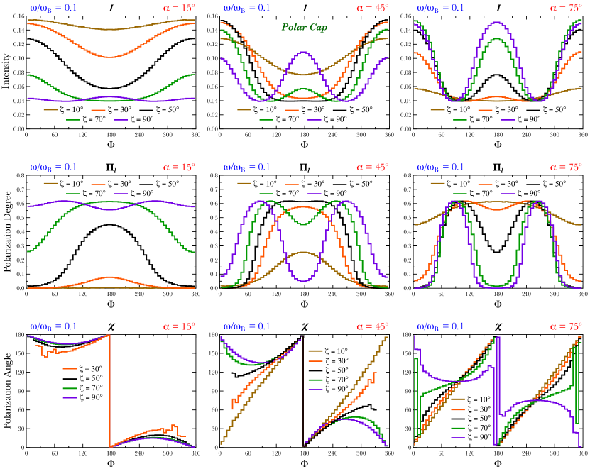
Figure 7: Pulse profiles for intensity $\,I\,$, linear polarization degree $\,\Pi_{l}\,$ and polarization angle $\,\chi\,$, top to bottom, simulated for a surface with uniform emission within two antipodal polar caps spanning colatitudes $\,0^{\circ}\leq\theta\leq\theta_{\rm cap}=30^{\circ}\,$ and $\,150^{\circ}\leq\theta\leq 180^{\circ}\,$ degrees. These are plotted as functions of the rotation phase $\,\Phi\,$ for selected viewing angles $\,\zeta=10^{\circ},30^{\circ},50^{\circ},70^{\circ}\,$ and $\,90^{\circ}\,$. Each column displays results for one of the three selected magnetic inclination angles $\,\alpha=15^{\circ},45^{\circ},75^{\circ}\,$, and the frequency of the photons is fixed so that $\,\omega/\omega_{\hbox{\fiverm B}}=0.1\,$ at the magnetic poles (in the LIF). Observe that the $\,\zeta\,$ polarization angle trace for $\,\alpha=15^{\circ}\,$ was omitted due to poor statistics when $\,\Pi\,$ is low; other traces are truncated, as discussed in the text.

5.2 Hot Polar Caps and Equatorial Belts

A central picture emerging from Sec. 5.1 is that if the entire surface radiates, then the pulse profiles exhibit only very small intensity variations, of the order of 10% or less. This is incompatible with numerous X-ray pulsar and magnetar observations, likely indicating that in such cases only moderate or small portions of the stellar surface dominate the contributions to the soft X-ray signals. To address this, two select cases will be considered here, one with two symmetric polar caps where the radiative surface uniformly samples magnetic colatitudes in the range $\,0^{\circ}\leq\theta\leq\theta_{\rm cap}\equiv 30^{\circ}\,$ and $\,150^{\circ}\leq\theta\leq 180^{\circ}\,$, and the other with an equatorial belt, where the active surface region uniformly spans the colatitudes $\,60^{\circ}\leq\theta\leq 120^{\circ}\,$. Polar caps are widely used for isolated neutron stars in the literature, notably in the offerings of Perna & Gotthelf (2008); Gotthelf et al. (2010); Albano et al. (2010); Bernardini et al. (2011); Younes et al. (2020); see the Introduction. Such regions are widely expected to be hotter on average due to the much higher thermal conductivities along magnetic fields – polar regions with vertical fields are more likely to conduct heat to atmospheres from thermal reservoirs deeper in the crust. Such is a strong motivation for adopting pole-centric surface temperature profiles with $\,T\,$ declining with colatitude as in Greenstein & Hartke (1983) and numerous subsequent works. Yet, the possibility that toroidal field components may exist near (e.g., Thompson et al., 2002, for magnetospheric twists) or in the stellar surface (e.g. Viganò et al., 2013, for sub-surface magneto-thermal models) in magnetars promotes prospects for heat transport away from polar zones to quasi-equatorial regions. Accordingly, equatorial belts are treated here to provide a contrasting case. Intuitively one expects these cases to exhibit stronger phase-dependent polarization signatures and intensity variations than for the uniform surface, and this is borne out in the simulation runs.

Fig. 7 displays the pulse profiles for intensity $\,I\,$, linear polarization degree $\,\Pi_{l}\,$ and polarization angle $\,\chi\,$ from a star with uniformly emitting polar caps ($\,0^{\circ}\leq\theta\leq 30^{\circ}\,$ and $\,150^{\circ}\leq\theta\leq 180^{\circ}\,$). The intensity variation is strongly enhanced with a typical pulsed fraction $\,\mathrel{\mathchoice{\lower 2.0pt\vbox{\halign{$\m@th\displaystyle\hfil#\hfil$\cr<\crcr\sim\crcr}}}{\lower 2.0pt\vbox{\halign{$\m@th\textstyle\hfil#\hfil$\cr<\crcr\sim\crcr}}}{\lower 2.0pt\vbox{\halign{$\m@th\scriptstyle\hfil#\hfil$\cr<\crcr\sim\crcr}}}{\lower 2.0pt\vbox{\halign{$\m@th\scriptscriptstyle\hfil#\hfil$\cr<\crcr\sim\crcr}}}}50\%\,$, contrasting the $\,10\%\,$ variation from the entire surface radiating case in Fig. 6. The pulse profiles of the linear polarization degree $\,\Pi_{l}\,$ for the polar cap case are similar to those presented in Fig. 6. Yet, the maximum $\,\Pi_{l}\,$ increases to around 60% when the instantaneous viewing angle $\,\theta_{v}\,$ to the $\,\hat{\bm{\mu}}_{\hbox{\fiverm B}}\,$ vector is close to 90$\,{}^{\circ}\,$, when on average, the observer views at large angles to the field directions at surface locales both proximate to the pole and near the equator. This large amplitude linear polarization is also present in previous polar cap models such as in the magnetar study of van Adelsberg & Perna (2009). The origin of the high $\,\Pi_{l}\,$ for polar caps that possess a constrained field morphology is in the reduction of the depolarization that naturally occurs when sampling a broad range of magnetic field directions from an entire surface. Such high polarizations are of great interest to future X-ray polarimetry observations and can be used to diagnose the geometric parameters ($\,\alpha,\zeta\,$) of the star. The polarization angle $\,\chi\,$ profiles for the polar cap case are similar to those displayed in Fig. 6. For some viewing directions, small $\,\Pi_{l}\,$ makes the $\,\chi\,$ profiles statistically noisy. These $\,\chi\,$ profiles are truncated for the $\,(\alpha=45^{\circ},\zeta=30^{\circ},50^{\circ})\,$ cases, and omitted for $\,\alpha=15^{\circ}\,$, $\,\zeta=10^{\circ}\,$, to improve the visualization.

While not explicitly displayed in Fig. 7, nor in Fig. 6, there is an inherent $\,\alpha\leftrightarrow\zeta\,$ interchange symmetry in the intensity and $\,\Pi_{l}\,$ pulse profiles that can be deduced by inspection of different panels in the upper two rows. This is manifested in the viewing angle relation in Eq. (12), and its origin is in the uniform sampling of magnetic azimuths on the surface. This symmetry can be appreciated by considering the $\,\Phi=0\,$ meridional plane where $\,\bm{\hat{\Omega}}\,$, $\,\hat{\bm{\mu}}_{\hbox{\fiverm B}}\,$ and $\,\hat{\bm{k}}_{{\fiverm{\infty}}}\,$ are coplanar; then there are two equivalent configurations with $\,\hat{\bm{\mu}}_{\hbox{\fiverm B}}\,$ and $\,\hat{\bm{k}}_{{\fiverm{\infty}}}\,$ swapped, essentially mirror images of each other. These are equivalent in terms of all the local magnetic orientations sampled by the curved photon trajectories that connect from the atmosphere to an observer at infinity. This $\,\alpha\leftrightarrow\zeta\,$ symmetry does not extend to the individual Stokes $\,Q\,$ and $\,U\,$ parameters, and therefore also not to the polarization angle $\,\chi\,$, as can be inferred from the bottom row of Fig. 7. For non-uniformity of the surface in magnetic azimuth, the degeneracy underlying this $\,\alpha\leftrightarrow\zeta\,$ symmetry is broken, and furthermore, significant distortion of the pulse profiles presented in the various figures will emerge.

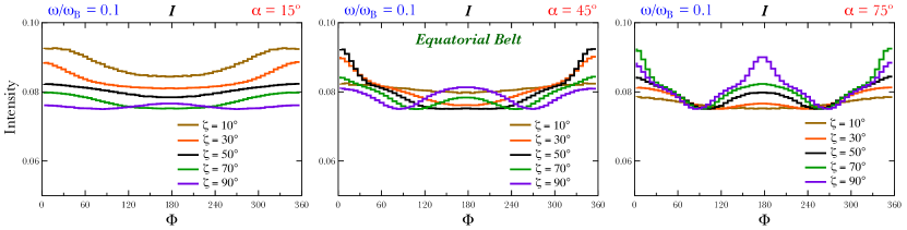
Figure 8: Simulated pulse profiles for intensity $\,I\,$ for an equatorial belt spanning colatitudes $\,60^{\circ}\leq\theta\leq 120^{\circ}\,$. For this case, the $\,\Pi_{l}\,$ and $\,\chi\,$ profiles are very similar to those for the full surfaces in Fig. 6, and so are not displayed here.

To contrast the polar cap example, Fig. 8 presents the intensity pulse profiles for the case where photons are emitted from an equatorial belt in the range $\,60^{\circ}\leq\theta\leq 120^{\circ}\,$, covering half of the whole stellar surface. The intensity profiles demonstrate modest variation, around 10% - 20%, marginally higher than for the entire surface emission example; this is not surprising as the equatorial belt represents half of the stellar surface. The $\,\Pi_{l}\,$ and $\,\chi\,$ traces for the equatorial belt are very similar to those in Fig. 6, with a maximum $\,\Pi_{l}\,$ around 50%; accordingly they are not displayed. The low pulse fraction of the equatorial belt is a direct consequence of the low-beaming intensity profiles at the corresponding colatitudes, as apparent in the atmosphere results presented in Fig. 2. In cases where soft X-ray observations of isolated neutron stars and magnetars exhibit much higher pulse fractions, this property of the atmosphere models indicates that polar cap locales for the origin of their signals below a few keV are likely preferred.

6 Discussion

A signature deliverable of the MAGTHOMSCATT code is its ability to accurately describe the anisotropies of radiative transfer for arbitrary field directions relative to the local zenith, and to do so in a computationally efficient manner using the high opacity injection protocol summarized in Section 2.2. Addressing non-vertical field directions is a non-trivial issue. The Monte Carlo approach accurately captures the inherent azimuthal asymmetry of photon escape around the B direction within the $\,\tau\mathrel{\mathchoice{\lower 2.0pt\vbox{\halign{$\m@th\displaystyle\hfil#\hfil$\cr<\crcr\sim\crcr}}}{\lower 2.0pt\vbox{\halign{$\m@th\textstyle\hfil#\hfil$\cr<\crcr\sim\crcr}}}{\lower 2.0pt\vbox{\halign{$\m@th\scriptstyle\hfil#\hfil$\cr<\crcr\sim\crcr}}}{\lower 2.0pt\vbox{\halign{$\m@th\scriptscriptstyle\hfil#\hfil$\cr<\crcr\sim\crcr}}}}1\,$ moderate opacity layer in the outer atmospheric slab. This asymmetry is intricately intertwined with pre- and post-scattering polarizations and photon directions, and strongly influences the values of the Stokes parameters. The degree of intensity beaming around B is also precisely modeled with the Monte Carlo technique, with Fig. 2 revealing prominent radiation collimation around the zenith at the magnetic poles when $\,\omega\ll\omega_{\hbox{\fiverm B}}\,$ that is not replicated at mid-latitude or equatorial locales. Such variations in local surface anisotropy profoundly impact the resultant intensity pulse profiles for rotating neutron stars.

The pulse profiles and sky maps presented in Section 5 are for monoenergetic photons, a restriction enabling clear discernment of principal characteristics. These plots demonstrate that if the entire star emits equally at all points on its surface, then the pulse fraction is generally small, as expected, and the phase-resolved linear polarization degree is modest, typically in the $\,5-20\,$% range. Both increase slightly when uniform emission in equatorial belts is explored (see Fig. 8), and are most pronounced when polar caps are modeled in Fig. 7. Specifically, for the uniform polar cap $\,\omega/\omega_{\hbox{\fiverm B}}=0.1\,$ illustration, pulse fractions of $\,30-60\,$% and linear polarization degrees of $\,\Pi_{l}\sim 20-60\,$% can be realized. These both decline somewhat when the frequency is increased to near and above the cyclotron frequency, though such behavior is not displayed in the various figures. All these characteristics are consequences of the fact that the magnetic Thomson cross section is more effective at polarizing and anisotropizing the radiation at $\,\omega\ll\omega_{\hbox{\fiverm B}}\,$ frequencies than at $\,\omega>\omega_{\hbox{\fiverm B}}\,$ frequencies, where the influence of the magnetic field is modest or small.

6.1 Soft X-ray Signatures for a Thermal Emission Case

In order for results from the MAGTHOMSCATT simulation to set the scene for future comparison with observed intensity and polarization pulse profiles, it is instructive to illustrate their characteristics by performing simulations in certain energy bands, encapsulating convolutions of monochromatic results like those presented in Secs. 5.1 and 5.2. Here we consider the thermal emission from antipodal $\,30^{\circ}\,$ polar caps of a neutron star, mirroring the geometry of Fig. 7, employing the standard parameters $\,M=1.44M_{\odot}\,$ and $\,R_{\hbox{\sixrm NS}}=10^{6}\,$ cm used throughout this paper. A Planck spectrum was assumed with a temperature satisfying $\,kT=0.42\,$ keV as measured by an observer at infinity. The polar caps were isothermal, so that the photon emission was uniformly sampled across the two caps. The polar field strength was $\,B_{p}=6.55\times 10^{10}\,$Gauss, as measured by an observer at infinity. Accordingly, in the local inertial frame at the stellar surface, the polar field was $\,B=9.74\times 10^{10}\,$ G ($\,\hbar\omega_{\hbox{\fiverm B}}=1.13\,$ keV), and the temperature satisfied $\,kT=0.55\,$ keV. At the rims of the polar caps, the field strength in the LIF was $\,B=8.88\times 10^{10}\,$Gauss ($\,\hbar\omega_{\hbox{\fiverm B}}=1.03\,$ keV). These parameters approximately generate the $\,\omega/\omega_{\hbox{\fiverm B}}\,$ values addressed in prior sections of the paper, and are suited to the pulse timing and spectral characteristics of the central compact object PSR J0821-4300 (Gotthelf et al., 2010, 2013).

The thermal simulations treated two separate energy bands sampled by an observer at infinity, $\,0.1-0.5\,$keV and $\,1-5\,$keV. For each of these, the LIF energy of each of the $\,2.5\times 10^{9}\,$ photons was uniformly sampled. A multiplicative weighting factor proportional to the Planck function was assigned to each photon according to its energy, and this factor was applied when recording the intensity and polarization information. The pulse profiles for intensity $\,I\,$ and linear polarization degree $\,\Pi_{l}\,$ for the simulation with photons in the $\,1-5\,$keV window are displayed in Fig. 9. The focus on this energy range was influenced by the fact that pulsars in the Galactic plane can be heavily absorbed at lower X-ray energies. In this case, $\,1.17\leq\omega/\omega_{\hbox{\fiverm B}}\leq 6.3\,$ in the LIF at all points on the two polar caps. The modulations of the intensity pulse profiles and linear polarization degrees are morphologically similar to the monochromatic case in Fig. 7. Yet, the intensity variation is diminished and the linear polarization degree $\,\Pi_{l}\,$ is reduced to $\,\mathrel{\mathchoice{\lower 2.0pt\vbox{\halign{$\m@th\displaystyle\hfil#\hfil$\cr<\crcr\sim\crcr}}}{\lower 2.0pt\vbox{\halign{$\m@th\textstyle\hfil#\hfil$\cr<\crcr\sim\crcr}}}{\lower 2.0pt\vbox{\halign{$\m@th\scriptstyle\hfil#\hfil$\cr<\crcr\sim\crcr}}}{\lower 2.0pt\vbox{\halign{$\m@th\scriptscriptstyle\hfil#\hfil$\cr<\crcr\sim\crcr}}}}20\%\,$, due to the general character of the cross section near and above the cyclotron resonance: see Barchas, Hu & Baring (2021). The pulsed fraction for intensity from our simulations varies from 0 to 17%, which is comparable to the 11% value measured in the $\,1.5-4.5\,$keV band for PSR J0821-4300 (Gotthelf et al., 2010). Moreover, the pulse shape is similar that for this pulsar, as displayed in Gotthelf et al. (2010, 2013), suggesting good prospects for employing our simulation to constrain stellar geometry parameters along the lines of several studies mentioned in the Introduction. The intensity and linear polarization degree results for the $\,0.1-0.5\,$keV energy band are very similar to those exhibited in Fig. 9, in both pulse shape and magnitudes, are therefore are not displayed explicitly.

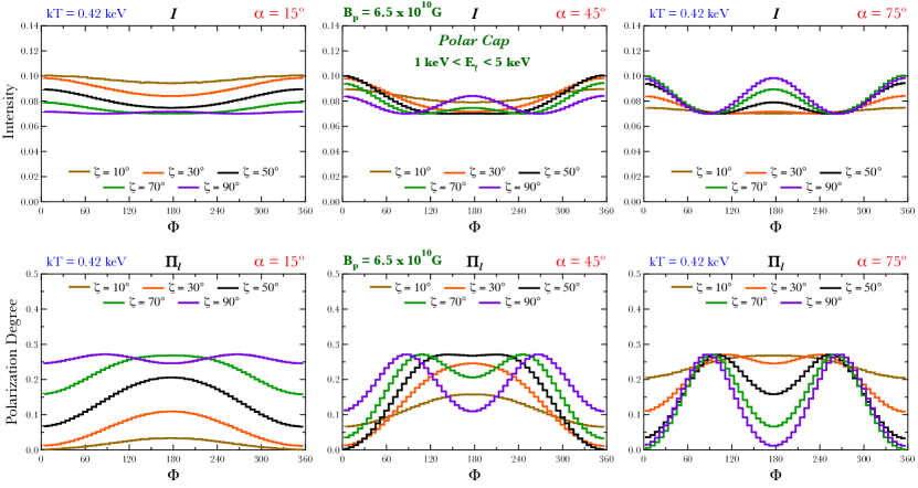
Figure 9: Frequency-integrated pulse phase profiles for intensity $\,I\,$ (top) and linear polarization degree $\,\Pi_{l}\,$ (bottom) for a uniformly emitting surface that consists of two antipodal polar caps spanning $\,30^{\circ}\,$ in colatitude as in Fig. 7. These are generated for a surface polar field of $\,B_{p}=6.5\times 10^{10}\,$Gauss (i.e., cyclotron energy $\,\approx 0.75\,$keV) and a Planck spectrum at temperature satisfying $\,kT=0.42\,$keV, both as perceived by an observer at infinity; the simulation distributed photons across the energy band $\,1-5\,$keV – see text. The profiles are plotted for selected viewing angles $\,\zeta=10^{\circ},30^{\circ},50^{\circ},70^{\circ}\,$ and $\,90^{\circ}\,$ to the spin axis. Each column displays results for one of the three selected magnetic inclination angles $\,\alpha=15^{\circ},45^{\circ},75^{\circ}\,$.

When source counts are limited, phase-integrated linear polarizations are generally the only obtainable polarization measures. In Table 1, we list two kinds of phase-averaged linear polarization degree information from our simulations for the different inclination and viewing angles depicted in Fig. 7. First, the phase-averaged linear polarization degree $\,\Pi^{\rm ave}_{l}=\sqrt{\langle Q\rangle^{2}+\langle U\rangle^{2}}/\langle I\rangle\,$ is calculated through accumulating the Stokes $\,Q\,$, $\,U\,$ and $\,I\,$ for all recorded photons regardless of their rotational phase $\,\Phi\,$. The average $\,\langle I\rangle\,$ is defined in Eq, (15), with similar definitions for $\,\langle Q\rangle\,$ and $\,\langle U\rangle\,$. The $\,\Pi^{\rm ave}_{l}\,$ values are around a few percent for most viewing directions, which are smaller than the typical phase-resolved linear polarization degrees presented in Fig 9. This is because the phase-resolved polarization angle $\,\chi\,$ is strongly dependent on $\,\Phi\,$, engendering strong cancellation in $\,Q/I\,$ and $\,U/I\,$ measures for different photons, which is signified by the alternating blue and red regions of the maps in Figs. 4 and 5. It is noticeable that $\,\Pi^{\rm ave}_{l}\,$ increases monotonically with increasing $\,\zeta\,$, a correlation that is driven by the observer generally viewing more obliquely to the surface field direction on average. When $\,\zeta\,$ is small, the viewer sees a polarization angle that rotates around the line of sight so that strong cancellation in both $\,Q\,$ and $\,U\,$ results when averaging over pulse phase.

As an alternative measure, the average of the phase-resolved linear polarization degree $\,\overline{\Pi}^{\rm pr}_{l}\,$ is defined as the average of the phase-dependent $\,\Pi_{l}\,$ values weighted by the intensity pulse profiles:

$$\overline{\Pi}^{\rm pr}_{l}\;\equiv\;\hbox{${{\displaystyle 1\vphantom{(}}\over{\displaystyle\langle I\rangle\vphantom{(}}}$}\int\sqrt{\bigl{[}Q(\Phi)\bigr{]}^{2}+\bigl{[}U(\Phi)\bigr{]}^{2}}\,\hbox{${{\displaystyle d\Phi\vphantom{(}}\over{\displaystyle 2\pi\vphantom{(}}}$}\quad,\quad\langle I\rangle\;=\;\int I(\Phi)\,\hbox{${{\displaystyle d\Phi\vphantom{(}}\over{\displaystyle 2\pi\vphantom{(}}}$}\quad.$$ (15)

The average $\,\overline{\Pi}^{\rm pr}_{l}\,$ gives the typical value of the phase-dependent linear polarization degree, and is in the range of $\,1-25\,$% for the cases listed in Table 1. Since there is no cancellation in the averaging process, $\,\overline{\Pi}^{\rm pr}_{l}\,$ is always greater than $\,\Pi^{\rm ave}_{l}\,$. Observe that while $\,\overline{\Pi}^{\rm pr}_{l}\,$ increases monotonically with $\,\zeta\,$ when $\,\alpha\leq 45^{\circ}\,$, it actually declines as $\,\zeta\,$ increases for the $\,\alpha=75^{\circ}\,$ simulations. This is a consequence of the fact that for large $\,\alpha\,$, perspectives with smaller $\,\zeta\,$ permit the observer to more often view more obliquely to the surface B direction, generating high $\,\Pi(\Phi)\,$. In contrast, large $\,\zeta\,$ for such quasi-perpendicular rotators leads to low values of $\,\Pi(\Phi)\,$ when the observer is looking almost parallel or anti-parallel to the local field direction, lowering $\,\overline{\Pi}^{\rm pr}_{l}\,$ accordingly. The fact that both polarization averages are higher for the $\,1-5\,$keV band than for the $\,0.1-0.5\,$keV band reflects a stronger partial cancellation of Stokes parameters in the sub-cyclotronic domain. With the launch of the IXPE mission this last December, phase-resolved polarization measurements, $\,\Pi_{l}(\Phi)\,$, of bright isolated neutron stars such as magnetars, will soon become available. Added to this library will be phase-averaged characteristics for relatively faint sources. This will allow us to confront our theoretical predictions with observationally determined polarization properties, thereby providing potential for discerning luminous atmospheric locations and neutron star geometry parameters in detail.

= 50mm

Table 1: Thermal Emission Simulations: Phase-averaged Linear Polarization Degrees

	$\,\alpha=15^{\circ}\,$				$\,\alpha=45^{\circ}\,$				$\,\alpha=75^{\circ}\,$
	0.1-0.5 keV		1-5 keV		0.1-0.5 keV		1-5 keV		0.1-0.5 keV		1-5 keV
	$\,\Pi^{\rm ave}_{l}\qquad\overline{\Pi}^{\rm pr}_{l}\,$		$\,\Pi^{\rm ave}_{l}\qquad\overline{\Pi}^{\rm pr}_{l}\,$		$\,\Pi^{\rm ave}_{l}\qquad\overline{\Pi}^{\rm pr}_{l}\,$		$\,\Pi^{\rm ave}_{l}\qquad\overline{\Pi}^{\rm pr}_{l}\,$		$\,\Pi^{\rm ave}_{l}\qquad\overline{\Pi}^{\rm pr}_{l}\,$		$\,\Pi^{\rm ave}_{l}\qquad\overline{\Pi}^{\rm pr}_{l}\,$
$\,\zeta=10^{\circ}\,$	0.0030	0.0095	0.0051	0.0168	0.0021	0.0810	0.0019	0.1112	0.0026	0.1866	0.0032	0.2409
$\,\zeta=30^{\circ}\,$	0.0302	0.0384	0.0450	0.0581	0.0123	0.0936	0.0152	0.1264	0.0202	0.1599	0.0257	0.2099
$\,\zeta=50^{\circ}\,$	0.0907	0.1021	0.1202	0.1355	0.0255	0.1104	0.1264	0.1509	0.0420	0.1252	0.0565	0.1662
$\,\zeta=70^{\circ}\,$	0.1571	0.1705	0.2029	0.2199	0.0398	0.1300	0.0529	0.1732	0.0599	0.0966	0.0806	0.1316
$\,\zeta=90^{\circ}\,$	0.1839	0.1975	0.2404	0.2583	0.0461	0.1393	0.0603	0.1827	0.0661	0.0861	0.0896	0.1187

6.2 Interpreting the Sky Maps: Stellar Geometry Diagnostics

The pattern structure of the sky maps serves as a fingerprint of the neutron star rotator geometry. The general appearance is governed by the loci of the zeros for the Stokes parameters that partition zones of opposite sign. The specification of these loci can be understood as follows. Due to the axial symmetry of the magnetic field configuration, the Stokes $\,Q\,$ equals zero when the projection of the magnetic axis $\,\hat{\bm{\mu}}_{\hbox{\fiverm B}}\,$ on the observer’s sky makes a 45$\,{}^{\circ}\,$ or 135$\,{}^{\circ}\,$ angle with the projection of the rotation axis $\,\bm{\hat{\Omega}}\,$ on the sky plane. The criteria can be expressed as $\,\hat{\bm{\mu}}_{\hbox{\fiverm B}}\cdot\hat{x}/\sin{\theta_{v}}=\pm 1/\sqrt{2}\,$, where $\,\hat{x}\,$ and $\,\theta_{v}\,$ are defined in Eq. (11) and Eq. (12). This relation can be simplified to

$$\sin{\alpha}\cos{\Phi}\cos{\zeta}-\cos{\alpha}\sin{\zeta}\;=\;\pm\sin{\alpha}\sin{\Phi}\quad,$$ (16)

where the $\,\pm\,$ sign on the right identifies the $\,\Phi\to 2\pi-\Phi\,$ symmetry of the geometry. As the star rotates, these criteria sample different $\,\zeta\,$ angles and trace two branches of white zero-value paths in the $\,\Phi-\zeta\,$ maps. Similarly, Stokes $\,U\,$ equals zero when the projection of the magnetic axis on the observer’s sky is parallel or orthogonal to the projection of the rotation axis on the sky, which yields $\,\hat{\bm{\mu}}_{\hbox{\fiverm B}}\cdot\hat{x}/\sin{\theta_{v}}=\pm 1\,$. This defines the morphology for the zero-value loci in the $\,U\,$ maps:

$$\sin{\Phi}\;=\;0\quad\text{or}\quad\tan{\zeta}\;=\;\tan{\alpha}\cos{\Phi}\quad,$$ (17)

with both relations encompassing $\,\Phi\to 2\pi-\Phi\,$ symmetry. Finally, the loci for $\,V=0\,$ constitute viewing directions where regions of opposite polarity are sampled equally across the stellar surface so that their emergent circular polarization signals precisely cancel. The only observer directions that satisfy this criterion for uniform surface illumination are those above the magnetic equator, so that the $\,V=0\,$ loci in Figs. 4 and 5 satisfy $\,\hat{\bm{\mu}}_{\hbox{\fiverm B}}\cdot\hat{\bm{k}}_{{\fiverm{\infty}}}=0\,$, i.e. $\,\theta_{v}=90^{\circ}\,$.

Observe that since these loci for zeros of the Stokes parameters depend only on the geometrical configuration of the three vectors $\,\bm{\hat{\Omega}}\,$, $\,\hat{\bm{k}}_{{\fiverm{\infty}}}\,$ and the precessing $\,\hat{\bm{\mu}}_{\hbox{\fiverm B}}\,$, they are independent of photon frequency, a property that is apparent when comparing Figs. 4 and 5; they are also independent of stellar mass and thus spacetime curvature. In principle, the determination of the phases for zeros of the Stokes Q and U parameters (or, equivalently, $\,\Pi_{l}\,$ and $\,\chi\,$) in concert with the intensity pulse profile provides powerful diagnostics on the stellar geometry parameters. Yet note that departures from azimuthal independence for the surface emission will introduce distortions to the shapes of these loci of zeros, thereby complicating the stellar parameter determination.

7 Conclusion

In this paper, we present our Monte Carlo simulation MAGTHOMSCATT that models radiation transport and scattering in atmospheric slabs, and generates intensity and polarization signatures from extended surface regions of magnetized neutron stars. The code captures the azimuthally asymmetric beaming and polarization information for each magnetic field orientation and generates pulse profiles for intensity and polarization signatures from extended atmospheres. This simulation of the magnetic Thomson scattering in high opacity environs is versatile, and can also be deployed in neutron star settings remote from their surfaces, for example to treat the accretion columns of X-ray pulsars and the transfer of radiation in bursts in magnetar magnetospheres. The code also implements general relativistic ray tracing and parallel transport of the Stokes parameters. These GR effects alter the observed intensity and polarization signals, changes that are apparent in $\,I,Q,U,V\,$ traces that are resolved in rotational phase; they therefore influence the determination of the stellar geometry parameters using phase-resolved observations. For a uniformly emitting star with $\,M=1.44M_{\odot}\,$, $\,R_{\hbox{\sixrm NS}}=10^{6}\,$ cm and $\,\omega/\omega_{\hbox{\fiverm B}}=0.1\,$, the effects of general relativity reduce the intensity variation from 30% to 6% (see Fig. 6), and change the general viewing direction for a maximum of intensity from $\,\theta_{v}=90^{\circ}\,$ in flat spacetime (roughly over the magnetic equator) to $\,\theta_{v}=0^{\circ}\,$ in GR, i.e. over the magnetic poles (see Fig. 6). We find that for a neutron star with uniformly emitting polar caps spanning a half angle $\,30^{\circ}\,$ in magnetic colatitude, the phase-resolved linear polarization degree can be as much as 60% for monochromatic photons.

To provide context for soft X-ray observations, we then simulated intensity and polarization signatures from the polar cap regions of a neutron star with parameters comparable to the central compact object PSR J0821-4300. This element considered photons from a Planck spectrum and assumed isothermal conditions across the polar caps. Photons in two energy bands were simulated, and the average linear polarization information was listed in Table 1. For this specific case, the phase-resolved linear polarization degree is generally in the range 10-25% when the viewing angle $\,\zeta\,$ is not too small, though the phase-averaged polarization is noticeably smaller, at the 1-20% level. Accordingly, it is clear that the phase-dependent polarization signatures from these simulations provide better prospects for exploitation using sensitive soft X-ray polarimeters in probing stellar geometry parameters. Future extensions of this work will focus on introducing hydrostatic structure to the atmosphere model. This will determine the temperature stratification in the outermost layers of the star and therefore define the interplay between polarization transport and photon frequencies that sample different physical depths within atmospheres. Free-free opacity, important at photon energies below around 2-3 keV, will also be incorporated, thereby modifying the transport from a purely magnetic Thomson one. In addition, the influences of vacuum birefringence on polarization transfer in twisted magnetospheres will be addressed. With these enhancements, our atmospheric radiative transfer code will be suited to addressing neutron star observations acquired by IXPE and future advanced X-ray polarimeters.

Appendix A: Magnetic Thomson Scattering Formalism

For the deployment of complex electric field vector information for photon transport in the slab, here we briefly summarize the key elements of the scattering: see Barchas, Hu & Baring (2021) for extensive details. The differential and total cross sections for a magnetic Thomson scattering are expressed in terms of the electric vectors of the incoming and outgoing electromagnetic waves. If the incident electromagnetic wave propagates in the direction of the unit vector $\,\hat{\bm{k}}_{i}\,$, the time portion of its electric field vector is encapsulated in $\,\bm{E}(t)=\bm{{\cal E}}_{i}e^{-i\omega t}\,$, with $\,\bm{{\cal E}}_{i}\cdot\hat{\bm{k}}_{i}=0\,$. The wave’s oscillating electric field accelerates the non-relativistic electron subject to the influence of a magnetic field $\,\bm{B}\equiv B\hat{\bm{B}}\,$. The motion is described by the Newton-Lorentz equation, whose solution generates an acceleration

$$\bm{a}\;=\;-\hbox{${{\displaystyle e\vphantom{(}}\over{\displaystyle m_{e}\vphantom{(}}}$}\,\hbox{${{\displaystyle\bm{\alpha}\,|\bm{{\cal E}}_{i}|\vphantom{(}}\over{\displaystyle\omega^{2}-\omega_{\hbox{\fiverm B}}^{2}\vphantom{(}}}$}\,e^{-i\omega t}\qquad\hbox{for}\qquad\bm{\alpha}\;=\;\omega^{2}\hat{\bm{{\cal E}}}_{i}-i\omega\omega_{\hbox{\fiverm B}}\,\hat{\bm{{\cal E}}}_{i}\times\hat{\bm{B}}-\omega_{\hbox{\fiverm B}}^{2}(\hat{\bm{{\cal E}}}_{i}\cdot\hat{\bm{B}})\hat{\bm{B}}\quad.$$ (18)

Here, $\,\omega_{\hbox{\fiverm B}}=eB/m_{e}c\,$ is the electron cyclotron frequency, and a scaled incident polarization vector $\,\hat{\bm{{\cal E}}}_{i}=\bm{{\cal E}}_{i}/|\bm{{\cal E}}_{i}|\,$ has been introduced to simplify ensuing expressions for the differential and total cross section. In general, $\,\hat{\bm{k}}_{i}\times\hat{\bm{B}}\neq\mathbf{0}\,$ so that $\,\bm{{\cal E}}_{i}\cdot\hat{\bm{B}}\neq\mathbf{0}\,$. The $\,\hat{\bm{{\cal E}}}_{i}\times\hat{\bm{B}}\,$ term in $\,\bm{\alpha}\,$ seeds circular polarization of the emergent wave, its influence being maximized near the cyclotron frequency; the other two terms precipitate linear polarization.

The electric field vector $\,\bm{{\cal E}}_{f}\,$ for the scattered (final) electromagnetic wave can quickly be written down using the non-relativistic dipole radiation formula (e.g., Rybicki & Lightman, 1979). As in Barchas, Hu & Baring (2021), here this polarization is expressed in normalized form, $\,\hat{\bm{{\cal E}}}_{f}=\bm{{\cal E}}_{f}/|\bm{{\cal E}}_{f}|\,$, and the differential cross section for magnetic Thomson scattering can be obtained as the ratio of Poynting fluxes for the final and initial waves:

$$\hat{\bm{{\cal E}}}_{f}\;\equiv\;\hbox{${{\displaystyle\bm{{\cal E}}_{f}\vphantom{(}}\over{\displaystyle|\bm{{\cal E}}_{i}|\vphantom{(}}}$}\;=\;\hbox{${{\displaystyle\hat{\bm{k}}_{f}\times\bigl{(}\hat{\bm{k}}_{f}\times\bm{\alpha}\bigr{)}\vphantom{(}}\over{\displaystyle\omega^{2}-\omega_{\hbox{\fiverm B}}^{2}\vphantom{(}}}$}\quad\Rightarrow\quad\hbox{${{\displaystyle d\sigma\vphantom{(}}\over{\displaystyle d\Omega_{f}\vphantom{(}}}$}\;=\;r_{0}^{2}\,\hat{\bm{{\cal E}}}_{f}\cdot\hat{\bm{{\cal E}}}_{f}^{*}\;=\;r_{0}^{2}\,\hbox{${{\displaystyle\bigl{(}\hat{\bm{k}}_{f}\times\bm{\alpha}\bigr{)}\cdot\bigl{(}\hat{\bm{k}}_{f}\times\bm{\alpha}^{\ast}\bigr{)}\vphantom{(}}\over{\displaystyle(\omega^{2}-\omega_{\hbox{\fiverm B}}^{2})^{2}\vphantom{(}}}$}\quad,$$ (19)

noting that this used the $\,|\hat{\bm{{\cal E}}}_{i}|=1\,$ normalization result. Here, $\,r_{0}=e^{2}/m_{e}c^{2}\,$ is the familiar classical electron radius. The full expression for $\,d\sigma/d\Omega_{f}\,$ in terms of the wave fields and directions can be found in Eq. (48) of Barchas, Hu & Baring (2021). It is routinely integrated over solid angles $\,\Omega_{f}\,$ for the scattered wave to yield the total cross section:

$$\sigma\;=\;\hbox{${{\displaystyle 8\pi\vphantom{(}}\over{\displaystyle 3\vphantom{(}}}$}\,r_{0}^{2}\,\hbox{${{\displaystyle\bm{\alpha}\cdot\bm{\alpha}^{\ast}\vphantom{(}}\over{\displaystyle(\omega^{2}-\omega_{\hbox{\fiverm B}}^{2})^{2}\vphantom{(}}}$}\;=\;\hbox{${{\displaystyle\sigma_{\hbox{\fiverm T}}\vphantom{(}}\over{\displaystyle(\omega^{2}-\omega_{\hbox{\fiverm B}}^{2})^{2}\vphantom{(}}}$}\biggl{[}\omega^{4}+\omega_{\hbox{\fiverm B}}^{2}(\omega_{\hbox{\fiverm B}}^{2}-2\omega^{2})\Bigl{|}\hat{\bm{{\cal E}}}_{i}\cdot\hat{\bm{B}}\Bigr{|}^{2}+\omega^{2}\omega_{\hbox{\fiverm B}}^{2}\Bigl{|}\hat{\bm{{\cal E}}}_{i}\times\hat{\bm{B}}\Bigr{|}^{2}+2i\,\omega^{3}\omega_{\hbox{\fiverm B}}\,\hat{\bm{B}}\cdot\bigl{(}\hat{\bm{{\cal E}}}_{i}\times\hat{\bm{{\cal E}}}_{i}^{*}\bigr{)}\biggr{]}\quad.$$ (20)

The various vector information contained in $\,\hat{\bm{{\cal E}}}_{i}\,$ and $\,\bm{B}\,$ describes the polarization configuration of the incident wave. For photons propagating in the $\,z\,$-direction we employ the Stokes parameter representation

$$\bm{{\cal E}}\;=\;{\cal E}_{x}\hat{x}+{\cal E}_{y}\hat{y}\;\equiv\;\bigl{|}\bm{{\cal E}}\bigr{|}\bigl{(}\hat{\cal E}_{x}\hat{x}+\hat{\cal E}_{y}\hat{y}\bigr{)}\quad\Rightarrow\quad\bm{S}\;\equiv\;\left(\begin{array}[]{c}I\\[2.0pt] Q\\[2.0pt] U\\[2.0pt] V\end{array}\right)\;=\;\left(\begin{array}[]{c}\langle{\cal E}_{x}{\cal E}_{x}^{*}\rangle+\langle{\cal E}_{y}{\cal E}_{y}^{*}\rangle\\[2.0pt] \langle{\cal E}_{x}{\cal E}_{x}^{*}\rangle-\langle{\cal E}_{y}{\cal E}_{y}^{*}\rangle\\[2.0pt] \langle{\cal E}_{x}{\cal E}_{y}^{*}\rangle+\langle{\cal E}_{x}^{*}{\cal E}_{y}\rangle\\[2.0pt] i\,\langle{\cal E}_{x}{\cal E}_{y}^{*}-{\cal E}_{x}^{*}{\cal E}_{y}\rangle\end{array}\right)\quad.$$ (21)

Here, $\,\hat{\cal E}_{x}={\cal E}_{x}/|\bm{{\cal E}}|\,$ and $\,\hat{\cal E}_{y}={\cal E}_{y}/|\bm{{\cal E}}|\,$, and the brackets $\,\langle\dots\rangle\,$ signify time averages of the products of wave field components. For particular surface locales, in Sec. 3 the coordinate axes are chosen using a reference plane coinciding with the local zenith axis $\,\hat{\bm{n}}\,$ and the photon propagation direction $\,\hat{\bm{k}}\,$. Specifically, $\,\hat{y}=\hat{\bm{n}}\times\hat{\bm{k}}/|\hat{\bm{n}}\times\hat{\bm{k}}|\,$ and $\,\hat{x}=\hat{y}\times\hat{\bm{k}}\,$. While this generates non-zero $\,U\,$ for individual photons, integrations over azimuthal angles around the zenith give $\,U=0\,$ on average due to the symmetry of scatterings relative to the $\,\hat{\bm{n}}\,$-$\,\bm{B}\,$ plane. For implementations involving extended surface regions, the focus of Section 5, the Cartesian coordinates are instead coupled to the rotation axis $\,\bm{\hat{\Omega}}\,$ and the observer direction $\,\hat{\bm{k}}_{\infty}\,$. In such circumstances, $\,U\,$ is generally not zero.

Appendix B: Field Geometry, Intensity and Ray Tracing

In this Appendix, we summarize two core general relativistic elements that impact the results presented in this paper – spacetime distortion of the magnetic field morphology and ray tracing for curved photon trajectories. Here we employ the general relativistic form of a vacuum dipole magnetic field in a Schwarzschild metric is detailed in Wasserman & Shapiro (1983); Muslimov & Tsygan (1986); Gonthier & Harding (1994). For observer frame polar coordinates $\,(r,\,\theta,\,\phi)\,$ prescribed relative to the instantaneous dipolar axis $\,\hat{\bm{\mu}}_{\hbox{\fiverm B}}\,$ (to be distinguished from the local polar coordinates used above for the photon atmospheric transport), the field in the local inertial frame (LIF) can be expressed as

$$\bm{B}_{\hbox{\fiverm GR}}\;=\;3\hbox{${{\displaystyle B_{p}R_{\hbox{\sixrm NS}}^{3}\vphantom{(}}\over{\displaystyle r_{s}^{3}\vphantom{(}}}$}\,\Psi^{3}\biggl{\{}\xi_{r}(\Psi)\,\cos\theta\,\hat{r}+\xi_{\theta}(\Psi)\,\sin\theta\,\hat{\theta}\biggr{\}}\quad,\quad\Psi\;=\;\hbox{${{\displaystyle r_{s}\vphantom{(}}\over{\displaystyle r\vphantom{(}}}$}\;\equiv\;\hbox{${{\displaystyle 2GM\vphantom{(}}\over{\displaystyle c^{2}r\vphantom{(}}}$}\quad,$$ (22)

at radius $\,r\,$, where $\,r_{s}=2GM/c^{2}\,$ is the Schwarzschild radius of a neutron star of mass $\,M\,$, whose radius is $\,R_{\hbox{\sixrm NS}}\,$. Thus $\,\Psi\,$ serves as the parameter for defining the redshift of the photon frequency in propagating from the surface to infinity. Throughout the paper, we set $\,M=1.44M_{\odot}\,$ and $\,R_{\hbox{\sixrm NS}}=10^{6}\,$ cm, so that $\,\Psi_{\hbox{\sixrm S}}=r_{s}/R_{\hbox{\sixrm NS}}\approx 0.425\,$ is the value of the trajectory radial parameter $\,\Psi=r_{s}/r\,$ at the surface. The scaling $\,B_{p}\,$ represents the flat spacetime value of the polar magnetic field at the surface. The field component functions are defined by

$$\xi_{r}(x)\;=\;-\frac{1}{x^{3}}\left[\log_{e}(1-x)+x+\frac{x^{2}}{2}\right]\quad,\quad\xi_{\theta}(x)\;=\;\frac{1}{x^{3}\sqrt{1-x}}\left[(1-x)\,\log_{e}(1-x)+x-\frac{x^{2}}{2}\right]\quad,$$ (23)

with $\,\xi_{r}(x)\approx 1/3\,$ and $\,\xi_{\theta}(x)\approx 1/6\,$ when $\,x\ll 1\,$ in flat spacetime, reproducing the familiar dipole form. The influence of general relativity is to enhance the magnetic field strength in the LIF. These forms were used to compute the field lines depicted in Fig. 1. By taking the ratio of the $\,\hat{\theta}\,$ and $\,\hat{r}\,$ components in Eq. (22), it is promptly determined that

$$\theta_{\hbox{\sixrm B}}\;=\;\arctan\left\{\hbox{${{\displaystyle\xi_{\theta}(\Psi)\vphantom{(}}\over{\displaystyle\xi_{r}(\Psi)\vphantom{(}}}$}\,\tan\theta\right\}$$ (24)

is the local zenith angle for the atmospheric magnetic field direction at any position on the neutron star surface, i.e., that indicated in the slab geometry on the left side of Fig. 1. It is routinely discerned that $\,\xi_{\theta}(\Psi)/\xi_{r}(\Psi)\,$ is an increasing function of $\,\Psi\,$, so that the Schwarzschild metric tilts the surface fields somewhat towards the local horizon.

In the Schwarzschild metric, for light emerging from the surface at a position $\,\bm{r}_{\hbox{\fiverm S}}=R_{\hbox{\sixrm NS}}\hat{\bm{r}}_{\hbox{\fiverm S}}\,$ relative to the star’s center in a direction $\,\hat{\bm{k}}_{\hbox{\fiverm S}}\,$ (its normalized wavector), the trajectory of the light ray lies in the plane defined by these two vectors. This plane also contains the unit radial vector $\,\hat{\bm{r}}_{\infty}\,$ from the center of the star to an observer at infinity, where $\,\hat{\bm{k}}\equiv\hat{\bm{k}}_{\infty}=\hat{\bm{r}}_{\infty}\,$ . The shape of the trajectory is specified by the impact parameter $\,b\,$, which represents the lateral distance offset between $\,\bm{r}_{\infty}\,$ and the asymptote of the trajectory at infinity. The impact parameter is related to the zenith angle $\,\theta_{z}\,$ of the photon in the LIF (satisfying $\,0\leq\theta_{z}\leq\pi/2\,$) as it leaves the atmospheric surface via

$$\Psi_{b}\;=\;\frac{r_{s}}{b}\;=\;\frac{\Psi_{\hbox{\sixrm S}}\sqrt{1-\Psi_{\hbox{\sixrm S}}}}{\sin{\theta_{z}}}\quad;$$ (25)

see Eq. (17) of Gonthier & Harding (1994). Clearly, there is a one-to-one correspondence between impact parameter and emission zenith angle. A schematic depiction of these vectors and the trajectory geometry is given in Fig. 3. The photon trajectory is most conveniently expressed using a single-branched elliptical integral for the orbital angle $\,\eta\,$ between the photon position vector $\,\bm{r}\,$ at $\,\Psi\,$ and the photon direction at infinity $\,\hat{\bm{r}}_{\infty}=\hat{\bm{k}}_{{\fiverm{\infty}}}\,$; the well-known result (e.g., Pechenick et al., 1983) is

$$\eta(\Psi)\;=\;\int^{\Psi}_{0}\frac{d\Psi_{r}}{\sqrt{\Psi^{2}_{b}-\Psi^{2}_{r}(1-\Psi_{r})}}\;\approx\;\arccos{\left(\hbox{${{\displaystyle\cos{\theta-\Psi}\vphantom{(}}\over{\displaystyle 1-\Psi\vphantom{(}}}$}\right)}\quad.$$ (26)

The exact trajectory is given by the integral form, and the approximation on the right of Eq. (26) is that obtained by Beloborodov (2002) that is accurate to $\,\mathrel{\mathchoice{\lower 2.0pt\vbox{\halign{$\m@th\displaystyle\hfil#\hfil$\cr<\crcr\sim\crcr}}}{\lower 2.0pt\vbox{\halign{$\m@th\textstyle\hfil#\hfil$\cr<\crcr\sim\crcr}}}{\lower 2.0pt\vbox{\halign{$\m@th\scriptstyle\hfil#\hfil$\cr<\crcr\sim\crcr}}}{\lower 2.0pt\vbox{\halign{$\m@th\scriptscriptstyle\hfil#\hfil$\cr<\crcr\sim\crcr}}}}1\%\,$, sufficient for our neutron star applications. Here, $\,\theta\,$ is the zenith angle of the photon momentum $\,\bm{k}_{\hbox{\fiverm GR}}\,$ in the local inertial frame at any radius, i.e. its angle to the radial direction. Thus, $\,\cos\theta=\bm{k}_{\hbox{\fiverm GR}}\cdot\hat{r}/|\bm{k}_{\hbox{\fiverm GR}}|\,$, which can be evaluated using the form for $\,\bm{k}_{\hbox{\fiverm GR}}\,$ posited in Eq. (41) of Story & Baring (2014):

$$\bm{k}_{\hbox{\fiverm GR}}\;=\;\hbox{${{\displaystyle|\bm{k}_{\infty}|\vphantom{(}}\over{\displaystyle\Psi_{b}\sqrt{1-\Psi}\vphantom{(}}}$}\left\{\sqrt{\Psi_{b}^{2}-\Psi^{2}(1-\Psi)}\,{\hat{r}}+\Psi\sqrt{1-\Psi}\,{\hat{\theta}}\right\}\quad\Rightarrow\quad\cos\theta\;=\;\hbox{${{\displaystyle 1\vphantom{(}}\over{\displaystyle\Psi_{b}\vphantom{(}}}$}\sqrt{\Psi_{b}^{2}-\Psi^{2}(1-\Psi)}\quad.$$ (27)

As the photon propagates to infinity, $\,\Psi\to 0\,$ and the polar component approaches zero. When $\,r=R_{\hbox{\sixrm NS}}\,$, ($\,\Psi=\Psi_{\hbox{\sixrm S}}\,$) and the value of $\,\eta_{\hbox{\fiverm S}}\equiv\eta(\Psi_{\hbox{\sixrm S}})\,$ is obtained using $\,\theta\to\theta_{z}\,$ in Eq. (26). Accordingly, there is a convenient coupling of the zenith angle intensity information from the atmospheric transport simulation and the GR propagation to infinity.

The GR propagation computation in MAGTHOMSCATT was tested by comparing the simulated photon trajectories with the exact solutions in Eq. (26). For $\,M=1.44M_{\odot}\,$, the directional precision at high altitudes was typically better than 0.1 degrees when the emission zenith angle satisfied $\,\theta_{z}\leq 60^{\circ}\,$ . This error grows if $\,\theta_{z}\,$ is increased, and reaches a maximum around 3.5 degrees (2.6%) at $\,\theta_{z}=90^{\circ}\,$. This precision is sufficient for the directional binning of 3$\,{}^{\circ}\,$ on the sky adopted in Figure. 4 and 5. We note that most emergent photons have small $\,\theta_{z}\,$ in the atmospheric intensity profiles. The cosine relation in Eq. (26) is valid for $\,\Psi_{\hbox{\sixrm S}}\,$ smaller than 0.5. This $\,\Psi_{\hbox{\sixrm S}}\,$ value corresponds to a mass around $\,1.7M_{\odot}\,$, above which the argument of the arccosine function exceeds $\,-1\,$. An alternative light bending empirical approximation developed by Poutanen (2020) gives more accurate results that can be used for stars with larger masses, ranging up to $\,2M_{\odot}\,$. Yet, above this mass, the error of Poutanen’s formula grows rapidly for large emission $\,\theta_{z}\,$. Both this and the Beloborodov (2002) approximation address the expected mass range for normal neutron stars.

A second test of the GR ray tracing implementation was made by investigating the visible stellar surface for an observer at infinity. For any observer, the visible surface is larger than for the flat spacetime case due to gravitational light bending, and for fixed radius it increases with greater stellar mass. The range of photon orbit angles $\,\eta_{\hbox{\fiverm S}}\,$ corresponding to the visible surface can be obtained using the integral in Eq. (26) by setting $\,\theta_{z}\,$ to 90$\,{}^{\circ}\,$, corresponding to emission parallel to the atmospheric horizon. Using the cosine relation one can quickly obtain the maximum orbit angle $\,\eta_{\rm max}\,$ such that $\,0\leq\eta_{\hbox{\fiverm S}}\leq\eta_{\rm max}\,$. It was determined that the simulation estimate for $\,\eta_{\rm max}\,$ agreed with the evaluation of the integral in Eq. (26) within an error of around 3.5 degrees (2.6%) for $\,M=1.44M_{\odot}\,$.

Appendix C: Numerical integration test for intensity and Stokes parameters

As an independent check on the GR propagation modules in the simulation, the light curves and Stokes parameters from a neutron star can be calculated using direct numerical integrations over the entire surface for specified surface anisotropy and polarization information. We consider a far away observer with a distance $\,r\rightarrow\infty\,$ from the star’s center. Following Beloborodov (2002), the observed flux can be expressed in our notations as

$$dF\;=\;(1-\Psi_{\hbox{\sixrm S}}){I_{\omega}}(\mu)\cos{\theta_{z}}\,\frac{d\cos{\theta_{z}}}{d\cos\eta_{\hbox{\fiverm S}}}\frac{dS}{r^{2}}\quad.$$ (28)

This equation is equivalent to Eq. (3.14) of Pechenick et al. (1983), and can also be derived from the analysis in Section II of Riffert & Mészáros (1988). Here the $\,1-\Psi_{\hbox{\sixrm S}}\,$ factor expresses the frequency redshift. The argument $\,\mu=\cos{\Theta_{\hbox{\sixrm kB}}}\,$ of the atmospheric intensity $\,I_{\omega}\,$ is the cosine of the angle between the photon momentum and the local magnetic field direction (see Sec. 2.2), noting that for this test, the injection is azimuthally symmetric about the local field B. Also, $\,\eta_{\hbox{\fiverm S}}\,$ is the colatitude of the emission locale measured relative to the observer direction $\,\hat{\bm{k}}_{{\fiverm{\infty}}}\,$, and $\,dS=\sin{\eta_{\hbox{\fiverm S}}}d\eta_{\hbox{\fiverm S}}d\phi_{\hbox{\fiverm k}}\,$ is an area element on the surface. The $\,dS/{r^{2}}\,$ factor reflects the inverse square flux dilution in flat spacetime. The Jacobian $\,d\cos{\theta_{z}}/d\cos{\eta_{\hbox{\fiverm S}}}\,$ can be solved numerically by differentiating the integral in Eq. (26), or analytically using Beloborodov’s cosine relation therein, which yields

$$F\;\approx\;\int(1-\Psi_{\hbox{\sixrm S}})^{2}{I_{\omega}}(\mu)\cos{\theta_{z}}\frac{dS}{r^{2}}\quad\hbox{since}\quad\hbox{${{\displaystyle d\cos{\theta_{z}}\vphantom{(}}\over{\displaystyle d\cos\eta_{\hbox{\fiverm S}}\vphantom{(}}}$}\;\approx\;(1-\Psi_{\hbox{\sixrm S}})\quad.$$ (29)

This comparison flux $\,F\,$ is integrated over the entire visible area on the surface. For radiation emitted from the whole stellar surface, the upper limit of the trajectory orbital angle $\,\eta_{\hbox{\fiverm S}}\,$ is $\,\eta_{\rm max}\approx\arccos{[-\Psi_{\hbox{\sixrm S}}/(1-\Psi_{\hbox{\sixrm S}})]}\,$. Thus the integrated flux $\,F\,$ is just a function of the viewing angle $\,\theta_{v}\,$, which varies for a fixed observer as the star rotates.

Similarly, the normalized Stokes parameters can be expressed in terms of the local surface Stokes parameters as

$$\begin{bmatrix}Q/I\\ U/I\\ V/I\end{bmatrix}\;{\approx}\;\frac{1}{F}\int\begin{bmatrix}Q\\ U\\ V\end{bmatrix}d\Omega\;{\approx}\;\frac{1}{F}\int(1-\Psi_{\hbox{\sixrm S}})^{2}{I_{\omega}}(\mu)\begin{bmatrix}\hat{Q}_{\omega}(\mu)\cos{2\delta}\\ \hat{Q}_{\omega}(\mu)\sin{2\delta}\\ \hat{V}_{\omega}(\mu)\end{bmatrix}\cos{\theta_{z}}\,\frac{dS}{r^{2}}\quad,$$ (30)

where $\,\delta\,$ is the angle between the reference frame axis at the observer position and the emission position reference axis parallel transported to the observer (see Eq. 11). To be precise, $\,\delta\,$ represents the angle of rotation from the local $\,\hat{x}\,$ direction (i.e., $\,\hat{\bm{B}}_{\hbox{\fiverm GR}}\times\hat{\bm{k}}_{\hbox{\fiverm S}}\,$) at the surface emission point to the $\,\hat{x}\,$ direction at infinity (i.e., $\,\bm{\hat{\Omega}}\times\hat{\bm{k}}_{{\fiverm{\infty}}}\,$); thus it depends on the local magnetic field direction $\,\hat{\bm{B}}_{\hbox{\fiverm GR}}\,$ and the viewing orbital angle $\,\eta_{\hbox{\fiverm S}}\,$. Here, the empirical Stokes expressions for $\,\hat{Q}_{\omega}\,$ and $\,\hat{V}_{\omega}\,$ in Eq. (2) are used for the surface Stokes values. Note that $\,\hat{U}_{\omega}\,$ is always zero due to our choice of Stokes parameter coordinate system at the surface, and the mapping of $\,\hat{Q}_{\omega}\,$ at the surface to a mixture of $\,Q\,$ and $\,U\,$ at infinity is connected to a standard rotation of coordinates through the angle $\,\delta\,$.

The test was executed for the dipole field configuration in the Schwarzschild metric using Eq. (1) and Eq. (2) to specify the intensity and polarization distribution function at each point on the emitting surface of the star. Thus, the test first employed the asymptotic solutions in domains of high opacity inside an atmosphere, with known mathematical character, instead of the full simulation. The flux and Stokes parameters accumulated over the whole visible surface, as measured by a far away observer, were then numerically integrated according to Eqs. (29) and (30). The intensity and polarization signatures obtained from the surface integrations depend on the inclination angle, viewing angle and the rotational phase of the star. To complete the test, these numerical integrations were then compared with a series of simulations with photons injected using Eq. (1) and Eq. (2) and $\,\tau_{{\hbox{\sixrm eff}}}=0\,$ for the entire surface. The injected photons thus undergo no scatterings in the simulation and are subsequently propagated directly to the observer through curved spacetime. The flux $\,F\,$, and Stokes $\,Q/I\,$, $\,U/I\,$, and $\,V/I\,$ from the simulations were obtained as functions of the instantaneous viewing angle $\,\theta_{v}\,$ for selected photon frequencies. These functions are in numerical agreement at the $\,\mathrel{\mathchoice{\lower 2.0pt\vbox{\halign{$\m@th\displaystyle\hfil#\hfil$\cr<\crcr\sim\crcr}}}{\lower 2.0pt\vbox{\halign{$\m@th\textstyle\hfil#\hfil$\cr<\crcr\sim\crcr}}}{\lower 2.0pt\vbox{\halign{$\m@th\scriptstyle\hfil#\hfil$\cr<\crcr\sim\crcr}}}{\lower 2.0pt\vbox{\halign{$\m@th\scriptscriptstyle\hfil#\hfil$\cr<\crcr\sim\crcr}}}}3\,$% level with those obtained from surface integration in Eq. (30), for a wide range of $\,\theta_{v}\,$ and $\,\omega\,$, thereby validating the general relativistic intensity and polarization propagation implementation in the simulation code.

References

- Abarr et al. (2020) Abarr Q., Baring M., Beheshtipour B., Beilicke M., de Geronimo G., Dowkontt P., Errando M., et al., 2020, ApJ, 891, 70. doi:10.3847/1538-4357/ab672c
- Albano et al. (2010) Albano, A., Turolla, R., Israel, G. L., et al. 2010, ApJ, 722, 788. doi:10.1088/0004-637X/722/1/788
- Barchas (2017) Barchas, J. A. 2017, PhD Thesis, Rice University.
- Barchas, Hu & Baring (2021) Barchas, J. A., Hu, K. & Baring, M. G. 2021, MNRAS, 500, 5369. doi:10.1093/mnras/staa3541
- Beloborodov (2002) Beloborodov, A. M. 2002, ApJ, 566, L85. doi:10.1086/339511
- Bernardini et al. (2011) Bernardini, F., Perna, R., Gotthelf, E. V., et al. 2011, MNRAS, 418, 638. doi:10.1111/j.1365-2966.2011.19513.x
- Braje et al. (2000) Braje, T. M., Romani, R. W., & Rauch, K. P. 2000, ApJ, 531, 447. doi:10.1086/308448
- Chandrasekhar (1960) Chandrasekhar, S. 1960, Radiative Transfer (Dover, New York)
- Chou (1986) Chou C. K., 1986, ApSS, 121, 333 doi:10.1007/BF00653705
- Fernández & Thompson (2007) Fernández, R., & Thompson, C. 2007, ApJ, 660, 615. doi:10.1086/511810
- Fernández & Davis (2011) Fernández, R., & Davis, S. W. 2011, ApJ, 730, 131. doi:10.1088/0004-637X/730/2/131
- Gonthier & Harding (1994) Gonthier, P. L. & Harding, A. K. 1994, ApJ, 425, 767 doi:10.1086/174020
- Gotthelf et al. (2010) Gotthelf, E. V., Perna, R., & Halpern, J. P. 2010, ApJ, 724, 1316. doi: 10.1088/0004-637X/724/2/1316
- Gotthelf et al. (2013) Gotthelf, E. V., Halpern, J. P., & Alford, J. 2013, ApJ, 765, 58. doi: 10.1088/0004-637X/765/1/58
- Greenstein & Hartke (1983) Greenstein, G. & Hartke, G. J. 1983, ApJ, 271, 283. doi:10.1086/161195
- Harding & Muslimov (1998) Harding, A. K. & Muslimov, A. G. 1998, ApJ, 500, 862. doi:10.1086/305763
- Harding & Kalapotharakos (2015) Harding, A. K. & Kalapotharakos, C. 2015, ApJ, 811, 63. doi:10.1088/0004-637X/811/1/63
- Harding & Kalapotharakos (2017) Harding, A. K. & Kalapotharakos, C. 2017, ApJ, 840, 73. doi:10.3847/1538-4357/aa6ead
- Heyl et al. (2003) Heyl, J. S., Shaviv, N. J., & Lloyd, D. 2003, MNRAS, 342, 134. doi: 10.1046/j.1365-8711.2003.06521.x
- Ho & Lai (2001) Ho, W. C. G., & Lai, D. 2001, MNRAS, 327, 1081. doi:10.1046/j.1365-8711.2001.04801.x
- Hu et al. (2019) Hu, K., Baring, M. G., Wadiasingh, Z., et al. 2019, MNRAS, 486, 3327. doi:10.1093/mnras/stz995
- Jahoda et al. (2019) Jahoda, K., Krawczynski, H., Kislat, F., et al. 2019, arXiv e-prints, arXiv:1907.10190.
- Lai & Ho (2003) Lai, D., & Ho, W. C. G. 2003, Phys. Rev. Lett, 91, 071101. doi:10.1103/PhysRevLett.91.071101
- Medin & Lai (2006) Medin, Z., Lai, D. 2006, Phys. Rev. A, 74, 062508 doi:10.1103/PhysRevA.74.062508
- Medin & Lai (2007) Medin, Z., Lai, D. 2007, MNRAS, 382, 1833 10.1111/j.1365-2966.2007.12492.x
- Mészáros (1992) Mészáros, P. 1992, High-energy Radiation from Magnetized Neutron Stars, (University of Chicago Press, Chicago)
- Mészáros & Bonazzola (1981) Mészáros P., & Bonazzola S., 1981, ApJ, 251, 695 doi:10.1086/159515
- Mészáros et al. (1988) Mészáros P., Novick R., Szentgyorgyi A., et al., 1988, ApJ, 324, 1056 doi:10.1086/165962
- Miller et al. (2019) Miller, M. C., Lamb, F. K., Dittmann, A. J., et al. 2019, ApJL, 887, L24 doi:10.3847/2041-8213/ab50c5
- Misner et al. (1973) Misner, C. W., Thorne, K. S., & Wheeler, J. A. 1973, Gravitation (San Francisco: W.H. Freeman and Co.)
- Muslimov & Tsygan (1986) Muslimov, A. G., & Tsygan, A. I. 1986, Sov. Astr. 30, 567
- Nobili et al. (2008) Nobili, L., Turolla, R., & Zane, S. 2008, MNRAS, 386, 1527. doi:10.1111/j.1365-2966.2008.13125.x
- Nollert et al. (1989) Nollert, H.-P., Ruder, H., Herold, H., & Kraus, U. 1989, A&A, 208, 153.
- Özel (2001) Özel, F. 2001, ApJ, 563, 276. doi:10.1086/323851
- Pavlov et al. (1994) Pavlov, G. G., Shibanov, Yu. A., Ventura, J., et al. 1994, A&A, 289, 837
- Pavlov & Zavlin (2000) Pavlov, G. G., & Zavlin, V. E. 2000, ApJ, 529, 1011. doi: 10.1086/308313
- Pechenick et al. (1983) Pechenick, K. R., Ftaclas, C., & Cohen, J. M. 1983, ApJ, 274, 846. doi:10.1086/161498
- Perna & Gotthelf (2008) Perna, R. & Gotthelf, E. V. 2008, ApJ, 681, 522. doi:10.1086/588211
- Pineault (1977) Pineault, S. 1977, MNRAS, 179, 691 doi: 10.1093/mnras/179.4.691
- Potekhin et al. (2004) Potekhin, A. Y., Lai, D., Chabrier, G., et al. 2004, ApJ, 612, 1034 doi:10.1086/422679
- Poutanen (2020) Poutanen, J. 2020, A&A, 640, A24 doi: 10.1051/0004-6361/202037471
- Psaltis et al. (2014) Psaltis, D., Özel, F., & Chakrabarty, D. 2014, ApJ, 787, 136. doi:10.1088/0004-637X/787/2/136
- Riffert & Mészáros (1988) Riffert, H. & Mészáros, P. 1988, ApJ, 325, 207. doi:10.1086/165996
- Riley et al. (2019) Riley, T. E., Watts, A. L., Bogdanov, S., et al. 2019, ApJL, 887, L21 doi:10.3847/2041-8213/ab481c
- Rybicki & Lightman (1979) Rybicki, G. B., & Lightman, A. P. 1979, Radiative Processes in Astrophysics (Wiley-Interscience, New York)
- Shibanov et al. (1992) Shibanov, Yu. A., Zavlin, V. E., Pavlov, G. G., et al. 1992, A&A, 266, 313
- Story & Baring (2014) Story, S. A. & Baring, M. G. 2014, ApJ, 790, 61 doi:10.1088/0004-637X/790/1/61
- Suleimanov et al. (2009) Suleimanov V., Potekhin A. Y., Werner K. 2009, A&A, 500, 891 doi:10.1051/0004-6361/200912121
- Taverna & Turolla (2017) Taverna, R. & Turolla, R. 2017, MNRAS, 469, 3610 doi:10.1093/mnras/stx1086
- Taverna et al. (2020) Taverna, R., Turolla, R., Suleimanov, V., et al. 2020, MNRAS, 492, 5057 doi:10.1093/mnras/staa204
- Thompson et al. (2002) Thompson, C., Lyutikov, M., & Kulkarni, S. R. 2002, ApJ, 574, 332 doi:10.1086/340586
- van Adelsberg & Lai (2006) van Adelsberg, M., Lai, D. 2006, MNRAS, 373, 1495 doi:10.1111/j.1365-2966.2006.11098.x
- van Adelsberg & Perna (2009) van Adelsberg, M., & Perna, R. 2009, MNRAS, 399, 1523 doi:10.1111/j.1365-2966.2009.15374.x
- Ventura, Nagel, & Mészáros (1979) Ventura J., Nagel W. & Mészáros P., 1979, ApJ, 233, L125 doi:10.1086/183090
- Viganò et al. (2013) Viganò, D., Rea, N., Pons, J. A., et al. 2013, MNRAS, 434, 123 doi:10.1093/mnras/stt1008
- Wasserman & Shapiro (1983) Wasserman, I. & Shapiro, S. L. 1983, ApJ, 265, 1036 doi:10.1086/160745
- Weinberg (1972) Weinberg, S. 1972, Gravitation and Cosmology: Principles and Applications of the General Theory of Relativity (Wiley & Sons, New York).
- Weisskopf et al. (2016) Weisskopf, M. C., Ramsey, B., O’Dell, S., et al. 2016, Proc. SPIE, 9905, 990517. doi:10.1117/12.2235240
- Whitney (1991a) Whitney, B. A. 1991, ApJ Supp., 75, 1293. doi:10.1086/191560
- Younes et al. (2020) Younes, G., Baring, M. G., Kouveliotou, C., et al. 2020, ApJ, 889, L27 doi:10.3847/2041-8213/ab629f
- Zane et al. (2000) Zane S., Turolla R., Treves A. 2000, ApJ, 537, 387 doi:10.1086/309027
- Zhang et al. (2016) Zhang, S. N., Feroci, M., Santangelo, A., et al. 2016, in Proc. SPIE, Vol. 9905. doi:10.1117/12.2232034