Structured model order reduction for vibro-acoustic problems using interpolation and balancing methods

Abstract

Vibration and dissipation in vibro-acoustic systems can be assessed using frequency response analysis. Evaluating a frequency sweep on a full-order model can be very costly, so model order reduction methods are employed to compute cheap-to-evaluate surrogates. This work compares structure-preserving model reduction methods based on rational interpolation and balanced truncation with a specific focus on their applicability to vibro-acoustic systems. Such models typically exhibit a second-order structure and their material properties as well as their excitation may be depending on the driving frequency. We show and compare the effectiveness of all considered methods by applying them to numerical models of vibro-acoustic systems depicting structural vibration, sound transmission, acoustic scattering, and poroelastic problems.

We give overviews about common system types arising from modeling of vibro-acoustic structures as well as state-of-the-art structure-preserving model reduction approaches based on interpolation and balanced truncation. The presented reduction methods are then employed and compared in efficiency on benchmark examples of the different vibro-acoustic structures.

1 Introduction

The numerical simulation of structural vibration, acoustic wave propagation, and their combination, often termed vibro-acoustic problems, is an important tool for many engineering applications. Especially, the prevention of unwanted noise or vibration is important in practice and many methods to dissipate surplus vibration energy have been established [40, 26, 22, 58]. These problems are typically evaluated by frequency sweeps. In the Laplace (frequency) domain, a vibro-acoustic system is described by linear systems of equations of the form

$$\Sigma\colon\begin{cases}\begin{aligned} \left(s^{2}\boldsymbol{\mathbf{M}}(s)+s\boldsymbol{\mathbf{C}}(s)+\boldsymbol{\mathbf{K}}(s)\right)\boldsymbol{\mathbf{x}}(s)&=\boldsymbol{\mathbf{F}}(s)\boldsymbol{\mathbf{u}}(s),\\ \boldsymbol{\mathbf{y}}(s)&=\boldsymbol{\mathbf{G}}\boldsymbol{\mathbf{x}}(s),\end{aligned}\end{cases}$$ (1)

with frequency-dependent matrix-valued functions $\boldsymbol{\mathbf{M}},\boldsymbol{\mathbf{C}},\boldsymbol{\mathbf{K}}\colon\mathbb{C}\rightarrow\mathbb{C}^{n\times n}$, describing the internal dynamics and representing mass, damping and stiffness, respectively, $\boldsymbol{\mathbf{F}}\colon\mathbb{C}\rightarrow\mathbb{C}^{n\times m}$, for the external forcing via the input $\boldsymbol{\mathbf{u}}(s)$, and the constant matrix $\boldsymbol{\mathbf{G}}\in\mathbb{R}^{p\times n}$, describing the quantities of interest as linear combinations of the system states. Therein, the controls $\boldsymbol{\mathbf{u}}\colon\mathbb{C}\rightarrow\mathbb{C}^{m}$ are used to steer the system state $\boldsymbol{\mathbf{x}}\colon\mathbb{C}\rightarrow\mathbb{C}^{n}$ to obtain the desired behavior of the outputs $\boldsymbol{\mathbf{y}}\colon\mathbb{C}\rightarrow\mathbb{C}^{p}$. Under the assumption that the system Eq. 1 is regular, i.e., there exists an $s\in\mathbb{C}$ for which the frequency-dependent functions can be evaluated and the center term for the (linear) dynamics, $\left(s^{2}\boldsymbol{\mathbf{M}}(s)+s\boldsymbol{\mathbf{C}}(s)+\boldsymbol{\mathbf{K}}(s)\right)$, is invertible, the input-to-output behavior of Eq. 1 is given by its transfer function

$$\boldsymbol{\mathbf{H}}(s) =\boldsymbol{\mathbf{G}}\left(s^{2}\boldsymbol{\mathbf{M}}(s)+s\boldsymbol{\mathbf{C}}(s)+\boldsymbol{\mathbf{K}}(s)\right)^{-1}\boldsymbol{\mathbf{F}}(s).$$ (2)

In practical applications, there is a demand for highly accurate models. Consequently, the number of equations in Eq. 1 quickly becomes very large ($n\gtrapprox 10^{5}$), which makes evaluation of Eq. 1 rather expensive in terms of computational resources such as time and memory. Model order reduction is a remedy to construct cheap-to-evaluate surrogate systems. In this paper, we consider structure-preserving model order reduction, i.e., the computed reduced-order model retains the original physically-inspired system structure of the full-order model or at least an interpretable equivalent. This has been shown to yield more accurate approximations if the reduced system’s order is low or allows even a physical re-interpreation of the reduced-order quantities. In case of vibro-acoustic systems Eq. 1, the reduced-order model should have the form

$$\hstretch{2}{\hat{\hstretch{.5}{\Sigma}}}\colon$$

with $\hstretch{2}{\hat{\hstretch{.5}{\boldsymbol{\mathbf{M}}}}},\hstretch{2}{\hat{\hstretch{.5}{\boldsymbol{\mathbf{C}}}}},\hstretch{2}{\hat{\hstretch{.5}{\boldsymbol{\mathbf{K}}}}}\colon\mathbb{C}\rightarrow\mathbb{C}^{r\times r}$, $\hstretch{2}{\hat{\hstretch{.5}{\boldsymbol{\mathbf{F}}}}}\colon\mathbb{C}\rightarrow\mathbb{C}^{r\times m}$ and $\hstretch{2}{\hat{\hstretch{.5}{\boldsymbol{\mathbf{G}}}}}\in\mathbb{C}^{p\times r}$, and a much smaller number of internal states and defining equations $r\ll n$. Its corresponding (reduced-order) transfer function is given by

$$\hstretch{2}{\hat{\hstretch{.5}{\boldsymbol{\mathbf{H}}}}}(s) =\hstretch{2}{\hat{\hstretch{.5}{\boldsymbol{\mathbf{G}}}}}\left(s^{2}\hstretch{2}{\hat{\hstretch{.5}{\boldsymbol{\mathbf{M}}}}}(s)+s\hstretch{2}{\hat{\hstretch{.5}{\boldsymbol{\mathbf{C}}}}}(s)+\hstretch{2}{\hat{\hstretch{.5}{\boldsymbol{\mathbf{K}}}}}(s)\right)^{-1}\hstretch{2}{\hat{\hstretch{.5}{\boldsymbol{\mathbf{F}}}}}(s).$$ (3)

To serve as surrogate, the reduced-order system Section 1 needs to approximate the original system’s input-to-output behavior, i.e., for the same input, the outputs of Eqs. 1 and 1 should be close to each other:

$$\left\lVert\boldsymbol{\mathbf{y}}-\hat{\boldsymbol{\mathbf{y}}}\right\rVert\leq\tau\cdot\left\lVert\boldsymbol{\mathbf{u}}\right\rVert,$$

with a tolerance $\tau$, in some appropriate norm and for all admissible inputs $\boldsymbol{\mathbf{u}}$. For frequency domain models, as they occur in vibro-acoustics, the approximation of the input-to-output behavior amounts to the approximation of the system’s transfer function in frequency regions of interest such that

$$\left\lVert\boldsymbol{\mathbf{H}}-\hstretch{2}{\hat{\hstretch{.5}{\boldsymbol{\mathbf{H}}}}}\right\rVert\leq\tau,$$

with the transfer functions from Eqs. 2 and 3.

The majority of system-theoretic model reduction techniques for dynamical systems can be classified as either based on system modes, interpolation or balancing of energy. Classically, modal approaches are used to solve structural and acoustic problems efficiently. These methods consider the solution of the system’s underlying eigenproblem to find poles of interest, which are retained in the reduced-order system. Modal methods are the classical, well-established approaches for the efficient reduction of vibro-acoustic systems and, therefor, we will not consider them further in this work. See [16] for a review on modal techniques for vibro-acoustic systems, [47] for the special case of systems with frequency-dependent material properties, and [56] for a new structured dominant pole-based approach for systems with modal damping.

Interpolation or moment-matching methods aim for low-order approximations that match the original transfer function behavior at certain expansion points. A general framework for structure-preserving interpolation of linear systems has been proposed in [8]. This approach can be immediately used for structured systems of the form Eq. 1, and has been applied to vibro-acoustic systems in [34]. For efficient numerical computations, ideas for Arnoldi-like algorithms have been extended to the second-order system case [6, 39] for application to structural and vibro-acoustic systems [5, 54, 59]. Further related methods for vibro-acoustic systems with poroelastic materials can be found in, e.g., [25, 49, 48]. An important aspect in interpolatory model order reduction is the choice of appropriate interpolation points. The iterative rational Krylov algorithm (IRKA) [32] computes interpolation point locations automatically. The resulting first-order systems are locally optimal in the sense of the approximation error’s $\mathcal{H}_{2}$-norm. Heuristic extensions for second-order systems with constant coefficient matrices have been proposed in, e.g., [57], and proven to provide good results in practice.

One of the most successful model reduction approaches for unstructured first-order systems is the balanced truncation method [44]. This approach considers the energy behavior of the system to identify parts of the state which contribute only marginally to the input-to-output behavior. Different extensions of heuristic nature have been proposed for second-order systems [43, 46, 19], which yield good results in practical applications [51]. More recently, new formulas have been proposed to limit the approximation behavior of the second-order balanced truncation methods in frequency or time domain to ranges of interest [13]. Extensive comparisons can be found in [56].

In this work, we present and compare different methods for reducing the numerical complexity of vibro-acoustic systems. Three main types of systems, which are encountered in the vibro-acoustic setting, are grouped regarding their damping and coupling behavior, and numerical benchmarks are given for each type. This allows a structured assessment of the applicability and the approximation quality of the employed methods. Here, we only consider interpolatory and balancing-related methods for second-order systems and do not include modal methods into our comparisons. Reviews and comparisons for such methods are given in [16, 51, 47, 56]. We identify, which reduction algorithms are applicable to a wide range of different systems without the need of problem specific modifications. The approximation quality is assessed by computing the MORscore [35], which yields a single number for each method on each benchmark example.

The rest of the article is organized as follows: In Section 2, we give an overview about numerical modeling of vibro-acoustic systems and group different application cases regarding the form of their transfer functions. The following Section 3 reviews the concepts of model order reduction methods we will use for the comparison. In Section 4, numerical models for all proposed types of vibro-acoustic systems are introduced and the performance of applicable reduction methods is compared. Section 5 concludes the article.

2 Types of vibro-acoustic systems

In this section, we describe the different system types occurring in the modeling of vibro-acoustic problems that we consider in this paper.

2.1 Structural dynamics

Structural vibration in spatial domains is often modeled using the finite element method (FEM). A discretization with finite elements leads to a system with the following transfer function

$$\boldsymbol{\mathbf{H}}(s) =\boldsymbol{\mathbf{G}}\left(s^{2}\boldsymbol{\mathbf{M}}+s\boldsymbol{\mathbf{C}}+\boldsymbol{\mathbf{K}}\right)^{-1}\boldsymbol{\mathbf{F}},$$ (4)

where the typically symmetric matrices $\boldsymbol{\mathbf{M}}$ and $\boldsymbol{\mathbf{K}}$ resemble the mass and stiffness of the model, respectively. The viscous damping, introduced by the damping matrix $\boldsymbol{\mathbf{C}}$, is often proportionally described, e.g., by Rayleigh damping. In this case, the corresponding damping matrix is a linear combination of the system’s mass and stiffness matrices and is given by

$$\boldsymbol{\mathbf{C}}_{\mathrm{R}}=\alpha\boldsymbol{\mathbf{M}}+\beta\boldsymbol{\mathbf{K}},$$

where the coefficients $\alpha$ and $\beta$ control the frequency region in which the structure is damped. Therein, $\alpha$ models the damping effect that the surrounding medium has on the structure, while $\beta$ accounts for the material damping.

The effect of proportional damping is not constant over the complete frequency range and the coefficients have to be tuned individually for each problem. A damping effect being constant for all frequencies can be described by structural damping, often introduced by a complex stiffness matrix. The corresponding frequency-dependent damping matrix is given by

$$\boldsymbol{\mathbf{C}}_{\mathrm{S}}(s)=\frac{\eta}{s}\mathrm{i}\boldsymbol{\mathbf{K}},$$

where $\eta$ is the structural loss factor, for which standard values are available for various materials. Discrete damping elements, for example dashpot dampers, can also be introduced in $\boldsymbol{\mathbf{C}}$. This results in a matrix structure, which is not proportional to mass or stiffness.

2.2 Acoustical modeling

Acoustic wave propagation is often modeled via the Helmholtz equation, which can also be discretized by finite elements. For bounded problems, for example inside a cavity, this leads to a transfer function of the form

$$\boldsymbol{\mathbf{H}}(s) =\boldsymbol{\mathbf{G}}\left(\frac{s^{2}}{c^{2}}\boldsymbol{\mathbf{M}}+s\boldsymbol{\mathbf{C}}+\boldsymbol{\mathbf{K}}\right)^{-1}\boldsymbol{\mathbf{F}}(s),$$ (5)

with $c$, the wave speed in the acoustic medium. The acoustic mass matrix $\boldsymbol{\mathbf{M}}$ represents the compressibility of the medium and the acoustic stiffness matrix $\boldsymbol{\mathbf{K}}$ its mobility. Damping is introduced, for example, by admittance boundary conditions such that the acoustic damping matrix $\boldsymbol{\mathbf{C}}$ is not proportional to $\boldsymbol{\mathbf{M}}$ or $\boldsymbol{\mathbf{K}}$. The three material matrices are typically symmetric. The frequency-dependent acoustic source term $\boldsymbol{\mathbf{F}}(s)$ introduces velocity or pressure sources into the system. Its frequency dependency is either linear or quadratic.

Unbounded problems depicting acoustic wave propagation in the open space can be modeled using different methods, such as absorbing boundary conditions (ABC), perfectly matched layers (PML), or infinite elements (IE) [37]. In these methods, the model is truncated at an arbitrarily chosen boundary, which is then treated in a way that Sommerfeld’s radiation condition is fulfilled. An example for an ABC is the Dirichlet-to-Neumann (DtN) condition, which imposes the analytical solution of the exterior domain on the arbitrary model boundary, leading to densely populated matrices [29]. IEs map the solution of decaying waves traveling outwards of the modeled domain to a finite set of nodes on which the numerical integration can be performed [4]. PMLs are absorbing layers added to the boundaries of the modeled domain. These layers ensure that waves can enter this region without being reflected at the boundary and are decaying inside the layer so they do not travel back into the domain of interest [15]. Introducing these conditions leads to a system with a damping matrix depending on the driving frequency of the system and transfer function

$$\boldsymbol{\mathbf{H}}(s) =\boldsymbol{\mathbf{G}}\left(\frac{s^{2}}{c^{2}}\boldsymbol{\mathbf{M}}+\boldsymbol{\mathbf{C}}\left(s\right)+\boldsymbol{\mathbf{K}}\right)^{-1}\boldsymbol{\mathbf{F}}(s).$$ (6)

The matrices resulting from a discretization with finite elements are complex symmetric and may for special cases be rewritten such that the frequency dependency can be separated. In case of PML, for example, it can be tuned for a specific frequency, such that the frequency dependency vanishes [55].

2.3 Vibro-acoustic systems

Coupling a vibrating structure with the surrounding acoustic fluid results in a vibro-acoustic system. The coupling is active in both ways: The vibrating structure radiates energy into the adjacent medium and is, in turn, excited by waves traveling through the acoustic fluid. Such systems are often used for modeling the sources of noise in machines or vehicles and to find ways to dissipate unwanted vibration or acoustic energy by introducing suitable damping. Examples for these mechanisms include poroelastic materials [17], constrained-layer damping [2], or mechanical joints [42]. The dissipation mechanisms are often governed by frequency-dependent complex-valued functions $\tilde{\phi}_{i}(s)$. Their influence on the model is given by corresponding constant matrices $\boldsymbol{\mathbf{C}}_{i}$ resulting in transfer functions of the form

$$\boldsymbol{\mathbf{H}}(s) =\boldsymbol{\mathbf{G}}\left(s^{2}\boldsymbol{\mathbf{M}}+s\boldsymbol{\mathbf{C}}+\boldsymbol{\mathbf{K}}+\sum\limits_{i=1}^{k}\tilde{\phi}_{i}(s)\boldsymbol{\mathbf{C}}_{i}\right)^{-1}\boldsymbol{\mathbf{F}}(s),$$

for some $k\in\mathbb{N}$. The coupling between the solid and fluid phases introduces off-diagonal terms in $\boldsymbol{\mathbf{M}}$ and $\boldsymbol{\mathbf{K}}$, making them non-symmetric. The frequency dependency of the input is only given, if the system is excited by an acoustic source. Structural excitation can be modeled by a constant input $\boldsymbol{\mathbf{F}}$.

2.4 Model problems

Although most vibro-acoustic systems are depicted as second-order systems, the different damping and coupling methods described above influence the structure of the transfer function, which may hinder the application of a specific reduction method. Therefor, we identify three types of model problems with varying properties, which will be reduced using applicable model order reduction techniques in the following:

Case A

A structural or interior vibro-acoustic system with proportional damping and no acoustic source following

$$\boldsymbol{\mathbf{H}}(s) =\boldsymbol{\mathbf{G}}\left(s^{2}\boldsymbol{\mathbf{M}}+s\left(d_{1}\boldsymbol{\mathbf{M}}+d_{2}\boldsymbol{\mathbf{K}}\right)+\boldsymbol{\mathbf{K}}\right)^{-1}\boldsymbol{\mathbf{F}},$$

where the damping factors $d_{1}$ and $d_{2}$ represent either Rayleigh or hysteretic damping. The resulting system matrices may be complex-valued if hysteretic damping is applied and non-symmetric for an interior vibro-acoustic problem.

Case B

An interior acoustic or vibro-acoustic system with acoustic source following

$$\boldsymbol{\mathbf{H}}(s) =\boldsymbol{\mathbf{G}}\left(\frac{s^{2}}{c^{2}}\boldsymbol{\mathbf{M}}+s\boldsymbol{\mathbf{C}}+\boldsymbol{\mathbf{K}}\right)^{-1}\boldsymbol{\mathbf{F}}(s).$$

An exterior radiation problem can also be modeled with this system type, if, for example, a PML is tuned to a single frequency.

Case C

An interior vibro-acoustic system with acoustic source and frequency-dependent material properties following

$$\boldsymbol{\mathbf{H}}(s) =\boldsymbol{\mathbf{G}}\left(s^{2}\boldsymbol{\mathbf{M}}+s\boldsymbol{\mathbf{C}}+\boldsymbol{\mathbf{K}}+\sum\limits_{i=1}^{k}\phi_{i}(s)\boldsymbol{\mathbf{C}}_{i}\right)^{-1}\boldsymbol{\mathbf{F}}(s),$$ (7)

where the frequency dependency can be described in an affine representation. The parameter dependency on the wave velocity $c$ is included in the entries of $\boldsymbol{\mathbf{M}}$ corresponding to the acoustic fluid. Again, exterior problems can be modeled, if the method ensuring Sommerfeld’s radiation condition can be represented by either a constant matrix or linear combination of matrices and corresponding frequency-dependent functions.

3 Model order reduction for vibro-acoustic systems

In this section, model order reduction methods for vibro-acoustic problems are considered. We begin with the general concept of projection-based model reduction and outline afterwards methods based on interpolation/moment matching and balancing.

3.1 Model reduction by projection

Consider linear systems of the form Eq. 1, which are described by their transfer functions Eq. 2. The goal of model reduction methods is now the construction of Section 1 such that the input-to-output behavior of Eq. 1 is approximated. The resulting main question is how to construct Section 1. In projection-based model reduction, two (constant) truncation matrices $\boldsymbol{\mathbf{V}},\boldsymbol{\mathbf{W}}\in\mathbb{C}^{n\times r}$ are constructed as bases of underlying projection spaces $\operatorname{span}(\boldsymbol{\mathbf{V}})$ and $\operatorname{span}(\boldsymbol{\mathbf{W}})$ such that the reduced-order quantities can be computed by

$$\begin{aligned} \hstretch{2}{\hat{\hstretch{.5}{\boldsymbol{\mathbf{M}}}}}(s)&=\boldsymbol{\mathbf{W}}^{\mathsf{H}}\boldsymbol{\mathbf{M}}(s)\boldsymbol{\mathbf{V}},&\hstretch{2}{\hat{\hstretch{.5}{\boldsymbol{\mathbf{C}}}}}(s)&=\boldsymbol{\mathbf{W}}^{\mathsf{H}}\boldsymbol{\mathbf{C}}(s)\boldsymbol{\mathbf{V}},&\hstretch{2}{\hat{\hstretch{.5}{\boldsymbol{\mathbf{K}}}}}(s)&=\boldsymbol{\mathbf{W}}^{\mathsf{H}}\boldsymbol{\mathbf{K}}(s)\boldsymbol{\mathbf{V}},\\ \hstretch{2}{\hat{\hstretch{.5}{\boldsymbol{\mathbf{F}}}}}(s)&=\boldsymbol{\mathbf{W}}^{\mathsf{H}}\boldsymbol{\mathbf{F}}(s),&\hstretch{2}{\hat{\hstretch{.5}{\boldsymbol{\mathbf{G}}}}}&=\boldsymbol{\mathbf{G}}\boldsymbol{\mathbf{V}};\end{aligned}$$ (8)

see, e.g., [3, 8]. In practice, the matrix functions in Eq. 8 have particular realizations from which the reduced-order models are built, e.g., the matrix function describing the mass of the system can always be realized in a frequency-affine decomposition

$$\boldsymbol{\mathbf{M}}(s) =\sum\limits_{k=1}^{n_{\mathrm{M}}}g_{k,\mathrm{M}}(s)\boldsymbol{\mathbf{M}}_{k},$$ (9)

with constant matrices $\boldsymbol{\mathbf{M}}_{k}\in\mathbb{C}^{n\times n}$, scalar frequency-dependent functions $g_{k,\mathrm{M}}\colon\mathbb{C}\rightarrow\mathbb{C}$ and usually $n_{\mathrm{M}}\ll n$. The reduced-order matrix function is then given by

$$\hstretch{2}{\hat{\hstretch{.5}{\boldsymbol{\mathbf{M}}}}}(s) =\boldsymbol{\mathbf{W}}^{\mathsf{H}}\boldsymbol{\mathbf{M}}(s)\boldsymbol{\mathbf{V}}=\sum\limits_{k=1}^{n_{\mathrm{M}}}g_{k,\mathrm{M}}(s)\boldsymbol{\mathbf{W}}^{\mathsf{H}}\boldsymbol{\mathbf{M}}_{k}\boldsymbol{\mathbf{V}}=\sum\limits_{k=1}^{n_{\mathrm{M}}}g_{k,\mathrm{M}}(s)\hstretch{2}{\hat{\hstretch{.5}{\boldsymbol{\mathbf{M}}}}}_{k},$$ (10)

with reduced-order matrices $\hstretch{2}{\hat{\hstretch{.5}{\boldsymbol{\mathbf{M}}}}}\in\mathbb{C}^{r\times r}$. In a similar way, the reduced matrix functions for the other terms in Eq. 8 are given. Since the scalar frequency-dependent functions in Eqs. 9 and 10 are the same, model order reduction by projection preserves the internal system structure in reduced-order models. Therefor, the reduced-order matrices in Eq. 10 can be used to replace their full-order counterparts to give a realization of the reduced-order model.

As a particular example, consider the classical second-order system Eq. 4. The reduced-order system is then given by the matrices

$$\begin{aligned} \hstretch{2}{\hat{\hstretch{.5}{\boldsymbol{\mathbf{M}}}}}&=\boldsymbol{\mathbf{W}}^{\mathsf{H}}\boldsymbol{\mathbf{M}}\boldsymbol{\mathbf{V}},&\hstretch{2}{\hat{\hstretch{.5}{\boldsymbol{\mathbf{C}}}}}&=\boldsymbol{\mathbf{W}}^{\mathsf{H}}\boldsymbol{\mathbf{C}}\boldsymbol{\mathbf{V}},&\hstretch{2}{\hat{\hstretch{.5}{\boldsymbol{\mathbf{K}}}}}&=\boldsymbol{\mathbf{W}}^{\mathsf{H}}\boldsymbol{\mathbf{K}}\boldsymbol{\mathbf{V}},&\hstretch{2}{\hat{\hstretch{.5}{\boldsymbol{\mathbf{F}}}}}&=\boldsymbol{\mathbf{W}}^{\mathsf{H}}\boldsymbol{\mathbf{F}},&\hstretch{2}{\hat{\hstretch{.5}{\boldsymbol{\mathbf{G}}}}}&=\boldsymbol{\mathbf{G}}\boldsymbol{\mathbf{V}}.\end{aligned}$$

However, with these specific construction rules for reduced-order models, the main question in projection-based model reduction is relocated to the actual construction of $\boldsymbol{\mathbf{V}}$ and $\boldsymbol{\mathbf{W}}$. The following sections give a short overview about the model reduction methods that will be used in the numerical experiments of this paper.

3.2 Moment matching and interpolation

A classical approach for choosing $\boldsymbol{\mathbf{V}}$ and $\boldsymbol{\mathbf{W}}$ as of Section 3.1 is by moment matching (interpolation) of the system’s transfer function. With the observation that classical linear systems, e.g., second-order systems of the form Eq. 4, have rational transfer functions, the idea of moment matching roots in the theory of Padé approximation [7, 18]. Thereby, rational Hermite interpolants of minimal degree in numerator and denominator are constructed. On the other hand, the moment matching method considers the representation of the transfer function in terms of a power series, for which the first coefficients are matched; see, e.g., [30, 24]. In a more general setting, all these ideas amount to the construction of the reduced-order model such that its corresponding transfer function solves a Hermite interpolation problem of the form

$$\frac{\mathrm{d}^{i_{j}}}{\mathrm{d}s^{i_{j}}}\boldsymbol{\mathbf{H}}(\sigma_{j}) =\frac{\mathrm{d}^{i_{j}}}{\mathrm{d}s^{i_{j}}}\hstretch{2}{\hat{\hstretch{.5}{\boldsymbol{\mathbf{H}}}}}(\sigma_{j}),$$ (11)

for $j=0,\ldots,k$ and $0\leq i_{j}\leq\ell_{j}$, in the interpolation points $\sigma_{1},\ldots,\sigma_{k}\in\mathbb{C}$. The most important result, in the computational sense, is that this interpolation Eq. 11 can be performed using the projection framework from Section 3.1; see, e.g., [31, 8]; which makes the moment matching approach well suited for use in many different applications. In the following, a quick overview about particular moment matching methods related to the system structure occurring in acoustic problems (Section 2) is given. For a more general introduction to interpolation and moment matching see also [3].

3.2.1 Second-order Arnoldi method

Krylov subspaces are often employed as valid choices for the projection subspaces $\operatorname{span}(\boldsymbol{\mathbf{V}})$ and $\operatorname{span}(\boldsymbol{\mathbf{W}})$. Their orthogonal bases $\boldsymbol{\mathbf{V}}$ and $\boldsymbol{\mathbf{W}}$ can, for example, be computed via an Arnoldi method [53, 5, 39]. For simplicity, we consider in this theoretic overview only systems with a single input and a single output (SISO), i.e., $\boldsymbol{\mathbf{F}}=\boldsymbol{\mathbf{f}}\in\mathbb{C}^{n}$ and $\boldsymbol{\mathbf{G}}=\boldsymbol{\mathbf{g}}\in\mathbb{C}^{n}$. For the application of the method to multi-input/multi-output (MIMO) systems see, e.g., [20]. The generalized $r$-th second-order Krylov subspace is defined by two matrices $\boldsymbol{\mathbf{A}},\boldsymbol{\mathbf{B}}\in\mathbb{C}^{n\times n}$ and a vector $\boldsymbol{\mathbf{v}}_{0}\in\mathbb{C}^{n}$ such that

$$\mathcal{S}_{r}\left(\boldsymbol{\mathbf{A}},\boldsymbol{\mathbf{B}};\boldsymbol{\mathbf{v}}_{0}\right) =\operatorname{span}\left(\boldsymbol{\mathbf{v}}_{0},\boldsymbol{\mathbf{v}}_{1},\dots,\boldsymbol{\mathbf{v}}_{r-1}\right),$$

where the recursively related vectors $\boldsymbol{\mathbf{v}}_{k}$ are given by

$$\begin{aligned} \boldsymbol{\mathbf{v}}_{1}&=\boldsymbol{\mathbf{A}}\boldsymbol{\mathbf{v}}_{0},\\ \boldsymbol{\mathbf{v}}_{i}&=\boldsymbol{\mathbf{A}}\boldsymbol{\mathbf{v}}_{i-1}+\boldsymbol{\mathbf{B}}\boldsymbol{\mathbf{v}}_{i-2}.\end{aligned}$$ (12)

The vectors in Eq. 12 are also known as the Krylov sequence based on $\boldsymbol{\mathbf{A}},\boldsymbol{\mathbf{B}},\boldsymbol{\mathbf{v}}_{0}$ and form the sought truncation matrix $\boldsymbol{\mathbf{V}}=\left[\boldsymbol{\mathbf{v}}_{0},\boldsymbol{\mathbf{v}}_{1},\dots,\boldsymbol{\mathbf{v}}_{r-1}\right]$. In order to find a basis, which projects the original system Eq. 4 onto a low-dimensional subspace such that the reduced system matches the first $r$ moments of the original system, the matrices and starting vector defining the Krylov sequence are set according to $\boldsymbol{\mathbf{A}}=-\boldsymbol{\mathbf{K}}^{-1}\boldsymbol{\mathbf{C}}$, $\boldsymbol{\mathbf{B}}=-\boldsymbol{\mathbf{K}}^{-1}\boldsymbol{\mathbf{M}}$ and $\boldsymbol{\mathbf{v}}_{0}=\boldsymbol{\mathbf{K}}^{-1}\boldsymbol{\mathbf{f}}$. The truncation matrix $\boldsymbol{\mathbf{W}}$ can be computed in the same way considering the adjoint problem.

If approximation around a specified frequency $s_{0}$ other than zero is desired, the transfer function can be shifted about this shift $s_{0}$ as in

$$H(s) =\boldsymbol{\mathbf{g}}\left((s-s_{0})^{2}\boldsymbol{\mathbf{M}}+(s-s_{0})\widetilde{\boldsymbol{\mathbf{C}}}+\widetilde{\boldsymbol{\mathbf{K}}}\right)^{-1}\boldsymbol{\mathbf{f}},$$

with $\widetilde{\boldsymbol{\mathbf{C}}}=2s_{0}\boldsymbol{\mathbf{M}}+\boldsymbol{\mathbf{C}}$ and $\widetilde{\boldsymbol{\mathbf{K}}}=s_{0}^{2}\boldsymbol{\mathbf{M}}+s_{0}\boldsymbol{\mathbf{C}}+\boldsymbol{\mathbf{K}}$. The corresponding $r$-th second-order Krylov subspace is then given by

$$\mathcal{S}_{r}\left(-\widetilde{\boldsymbol{\mathbf{K}}}^{-1}\widetilde{\boldsymbol{\mathbf{C}}},-\widetilde{\boldsymbol{\mathbf{K}}}^{-1}\boldsymbol{\mathbf{M}};\widetilde{\boldsymbol{\mathbf{K}}}^{-1}\boldsymbol{\mathbf{f}}\right).$$

The choice of the subspace dimension $r$ and location of the shift has a large influence on the approximation quality of the reduced model. To obtain a reduced-order model with a high accuracy for a wide range of frequencies, it usually is beneficial to not only increase the size of the Krylov subspace to match higher-order moments, but to combine multiple subspaces with different shifts into a global basis.

3.2.2 Structure-preserving interpolation

A more general approach for moment matching of structured linear systems is described in [8]. Any matrix-valued function of the form

$$\boldsymbol{\mathbf{H}}(s) =\boldsymbol{\mathcal{G}}(s)\boldsymbol{\mathcal{K}}(s)^{-1}\boldsymbol{\mathcal{F}}(s),$$ (13)

with $\boldsymbol{\mathcal{G}}\colon\mathbb{C}\rightarrow\mathbb{C}^{p\times n}$, representing the outputs, $\boldsymbol{\mathcal{K}}\colon\mathbb{C}\rightarrow\mathbb{C}^{n\times n}$, for the internal dynamics, and $\boldsymbol{\mathcal{F}}\colon\mathbb{C}\rightarrow\mathbb{C}^{n\times m}$, describing the system inputs, can be structure-preserving interpolated by projection. Given the two basis matrices $\boldsymbol{\mathbf{V}},\boldsymbol{\mathbf{W}}\in\mathbb{C}^{n\times r}$ of underlying right and left projection spaces, the reduced-order model is computed similarly to Eq. 8 by

$$\begin{aligned} {\hstretch{2}{\hat{\hstretch{.5}{\boldsymbol{\mathcal{G}}\mkern 1.0mu}}}\mkern-1.0mu}{}(s)&=\boldsymbol{\mathcal{G}}(s)\boldsymbol{\mathbf{V}},&{\hstretch{2}{\hat{\hstretch{.5}{\boldsymbol{\mathcal{K}}\mkern 1.0mu}}}\mkern-1.0mu}{}(s)&=\boldsymbol{\mathbf{W}}^{\mathsf{H}}\boldsymbol{\mathcal{K}}(s)\boldsymbol{\mathbf{V}},&{\hstretch{2}{\hat{\hstretch{.5}{\boldsymbol{\mathcal{F}}\mkern 1.0mu}}}\mkern-1.0mu}{}(s)&=\boldsymbol{\mathbf{W}}^{\mathsf{H}}\boldsymbol{\mathcal{F}}(s).\end{aligned}$$ (14)

The case of acoustic systems Eq. 1 is a special instance of Eq. 13, and particular realizations of Eq. 14 are computed using the same idea of frequency-affine decompositions as in Eqs. 9 and 10. With the same arguments, projection methods based on Eq. 14 are guaranteed to preserve the internal system structure. To give a concise overview, the following proposition states the most important result from [8] to solve Eq. 11 for systems of the form Eq. 13.

Proposition 1 (Structured interpolation [8, Theorem 1]).

Let $\boldsymbol{\mathbf{H}}$ be the transfer function of a linear system, described by Eq. 13, and $\hstretch{2}{\hat{\hstretch{.5}{\boldsymbol{\mathbf{H}}}}}$ the reduced-order transfer function constructed by projection Eq. 14. Let the matrix functions $\boldsymbol{\mathcal{G}}$, $\boldsymbol{\mathcal{K}}^{-1}$, $\boldsymbol{\mathcal{F}}$ and ${\hstretch{2}{\hat{\hstretch{.5}{\boldsymbol{\mathcal{K}}\mkern 1.0mu}}}\mkern-1.0mu}{}^{-1}$ be analytic in the interpolation point $\sigma\in\mathbb{C}$, and let $k,\theta\in\mathbb{N}_{0}$ be derivative orders.

1. If $\operatorname{span}\big{(}\frac{\mathrm{d}^{j}}{\mathrm{d}s^{j}}(\boldsymbol{\mathcal{K}}^{-1}\boldsymbol{\mathcal{F}})(\sigma)\big{)}\subseteq\operatorname{span}(\boldsymbol{\mathbf{V}})$, for $j=0,\ldots,k$, then it holds

   $$\frac{\mathrm{d}^{j}}{\mathrm{d}s^{j}}\boldsymbol{\mathbf{H}}(\sigma) =\frac{\mathrm{d}^{j}}{\mathrm{d}s^{j}}\hstretch{2}{\hat{\hstretch{.5}{\boldsymbol{\mathbf{H}}}}}(\sigma), \text{for}\leavevmode\nobreak\ j=0,\ldots,k.$$

2. If $\operatorname{span}\big{(}\frac{\mathrm{d}^{i}}{\mathrm{d}s^{i}}(\boldsymbol{\mathcal{K}}^{-\mathsf{H}}\boldsymbol{\mathcal{G}}^{\mathsf{H}})(\sigma)\big{)}\subseteq\operatorname{span}(\boldsymbol{\mathbf{W}})$, for $i=0,\ldots,\theta$, then it holds

   $$\frac{\mathrm{d}^{i}}{\mathrm{d}s^{i}}\boldsymbol{\mathbf{H}}(\sigma) =\frac{\mathrm{d}^{i}}{\mathrm{d}s^{i}}\hstretch{2}{\hat{\hstretch{.5}{\boldsymbol{\mathbf{H}}}}}(\sigma), \text{for}\leavevmode\nobreak\ i=0,\ldots,\theta.$$

3. If $\boldsymbol{\mathbf{V}}$ and $\boldsymbol{\mathbf{W}}$ are constructed as in Parts (a) and (b), then, additionally, it holds

   $$\frac{\mathrm{d}^{j}}{\mathrm{d}s^{j}}\boldsymbol{\mathbf{H}}(\sigma) =\frac{\mathrm{d}^{j}}{\mathrm{d}s^{j}}\hstretch{2}{\hat{\hstretch{.5}{\boldsymbol{\mathbf{H}}}}}(\sigma), \text{for}\leavevmode\nobreak\ j=0,\ldots,k+\theta+1.$$

Proposition 1 shows that only linear systems of equations need to be solved to construct an interpolating structure-preserving reduced-order model. However, the usual question that remains for interpolation methods is the choice of interpolation points. Over time, there have been many different attempts for heuristics strategies for how to choose interpolation points. The following ones will be used in this paper.

A very classical choice are points on the frequency axis $\mathrm{i}\mathbb{R}$. Depending on the frequency range of interest that is considered, the points are often chosen either linearly or logarithmically equidistant. This idea serves usually an overall reasonable approximation behavior but easily misses features of the system, which are not close enough to the interpolation points. In engineering sciences, this is then supplemented by educated guesses of points in frequency regions, which may be of certain importance due to additional knowledge about the modeling of the system.

As a more sophisticated choice of interpolation points, methods have been developed to minimize the approximation error in different systems norms. The worst case approximation error is described by the $\mathcal{H}_{\infty}$-norm. Therefor, large-scale computation methods [52, 1] and error estimators [27] can be used to determine successively new interpolation points minimizing the $\mathcal{H}_{\infty}$-error in a greedy algorithm [10]. On the other hand, there is the iterative rational Krylov algorithm (IRKA) for unstructured first-order systems, which solves the best approximation problem in the $\mathcal{H}_{2}$-norm [32]. There is no extension for the general setting Eq. 13 in a structure-preserving fashion. However, the transfer function IRKA (TF-IRKA) can be used to construct an optimal unstructured (first-order) $\mathcal{H}_{2}$-approximation for arbitrary transfer functions [9]. It has been shown to be very effective to use the final optimal interpolation points from TF-IRKA in the structure-preserving interpolation setting (Proposition 1). This basically resembles some of the ideas from [57] for an extension of the IRKA method to second-order systems.

A common drawback of interpolation methods is their global error behavior. While these methods are exact in the interpolation points, the surrounding error behavior may strongly differ depending on the actual transfer function. While it might help to also match several derivatives in the interpolation points using Proposition 1, a quite often used approach is the averaging or approximation of the constructed subspaces. The general idea is to compute the solution to the linear systems in Proposition 1 for a large amount of interpolation points, and then to approximate the resulting large projection spaces by lower-order ones. This can be done using, e.g., the pivoted QR decomposition or the singular value decomposition (SVD); see, e.g., [56] for more details. It has been shown in [11] that this oversampling procedure can be used to recover the controllability and observability subspaces of general systems like Eq. 13. Using some additional matrix products of the resulting basis matrices with the system matrices, the authors of [11] can compute minimal realizations of (linear) dynamical systems. Additional truncation of the resulting reduced-order matrices has been shown to still yield good results and is closely related to the idea of approximate subspaces.

3.3 AAA approximation of frequency-dependent functions

The contributions of general nonlinear frequency-dependent functions acting on parts of the system denoted by a set of constant matrices $\boldsymbol{\mathbf{C}}_{i}$ have to be considered for problems of type Eq. 7 from Case C in Section 2.4. To efficiently apply the structure-preserving interpolation framework from Section 3.2.2 to such models, the matrix functions in Eq. 13 can be represented by a series expansion about an interpolation point $s_{0}$:

$$\begin{aligned} \boldsymbol{\mathcal{K}}\left(s+s_{0}\right)&=\sum\limits_{\ell=0}^{\infty}s_{0}^{\ell}\boldsymbol{\mathcal{K}}_{\ell},&\boldsymbol{\mathcal{F}}\left(s+s_{0}\right)&=\sum\limits_{\ell=0}^{\infty}s_{0}^{\ell}\boldsymbol{\mathcal{F}}_{\ell},&\boldsymbol{\mathcal{G}}\left(s+s_{0}\right)=\sum\limits_{\ell=0}^{\infty}s_{0}^{\ell}\boldsymbol{\mathcal{G}}_{\ell}.\end{aligned}$$ (15)

While the series expansion factors can be computed straightforwardly for polynomials, general nonlinear functions require special treatment.

In the following approach, the required series expansion factors are computed from AAA approximations of the frequency-dependent functions. AAA computes a rational interpolant $r(s)$ of a complex-valued function $\phi(s)$ given function evaluations only [45]. The approximant $r(s)$ is originally given in barycentric form

$$r\left(s\right) =\frac{\sum\limits_{j=1}^{q}\frac{w_{j}f_{j}}{s-s_{j}}}{\sum\limits_{j=1}^{q}\frac{w_{j}}{s-s_{j}}},$$

where $q\geq 1$ is the order of approximation, $w_{j}$ are weights, $f_{j}$ are data points, and $s_{j}$ are support points. The barycentric form can be written in matrix notation as

$$r\left(s\right)=\boldsymbol{\mathbf{a}}\left(\boldsymbol{\mathbf{D}}+s\boldsymbol{\mathbf{E}}\right)^{-1}\boldsymbol{\mathbf{b}}$$

with

$$\begin{aligned} \boldsymbol{\mathbf{a}}&=\begin{bmatrix}w_{1}f_{1}&\cdots&w_{q}f_{q}\end{bmatrix},&\boldsymbol{\mathbf{b}}&=\begin{bmatrix}1&0&\cdots&0\end{bmatrix}^{\mkern-1.5mu\mathsf{T}},\\ \boldsymbol{\mathbf{D}}&=\begin{bmatrix}w_{1}&w_{2}&\cdots&w_{q-1}&w_{q}\\ -s_{1}&s_{2}&&&\\ &-s_{2}&\ddots&&\\ &&\ddots&s_{q-1}&\\ &&&-s_{q-1}&s_{q}\end{bmatrix},&\boldsymbol{\mathbf{E}}&=\begin{bmatrix}0&0&\cdots&0&0\\ 1&-1&&&\\ &1&\ddots&&\\ &&\ddots&-1&\\ &&&1&-1\end{bmatrix}.\end{aligned}$$

Shifting about $s_{0}$ yields

$$r(s) =\boldsymbol{\mathbf{a}}\left(\boldsymbol{\mathbf{I}}_{q}-\left(s-s_{0}\right)\widetilde{\boldsymbol{\mathbf{D}}}\right)^{-1}\tilde{\boldsymbol{\mathbf{b}}},$$ (16)

with $\widetilde{\boldsymbol{\mathbf{D}}}=-\left(\boldsymbol{\mathbf{D}}+s_{0}\boldsymbol{\mathbf{E}}\right)^{-1}\boldsymbol{\mathbf{E}}$, $\tilde{\boldsymbol{\mathbf{b}}}=\left(\boldsymbol{\mathbf{D}}+s_{0}\boldsymbol{\mathbf{E}}\right)^{-1}\boldsymbol{\mathbf{b}}$, and the $q$-dimensional identity matrix $\boldsymbol{\mathbf{I}}_{q}$; see [38]. The involved matrix inverse is computationally inexpensive, as $q$ is typically small. This procedure has to be performed for all $k$ functions $\phi_{i}(s)$, yielding a set of two vectors and a matrix $\{\boldsymbol{\mathbf{a}}_{i},\tilde{\boldsymbol{\mathbf{b}}}_{i},\widetilde{\boldsymbol{\mathbf{D}}}_{i}\}_{i=1}^{k}$ for each $\phi_{i}(s)$. Expanding Eq. 16 into a Neumann series for all $k$ functions $\phi_{i}(s)$ from Eq. 7 yields the sought after expansion factors for Eq. 15. For a Case C transfer function Eq. 7 and $\ell=2$, the series expansion of $\mathcal{K}_{\ell}$ in terms of Eq. 15 is given by

$$\begin{aligned} \boldsymbol{\mathcal{K}}_{0}&=s_{0}^{2}\boldsymbol{\mathbf{M}}+s_{0}\boldsymbol{\mathbf{C}}+\boldsymbol{\mathbf{K}}+\sum\limits_{i=0}^{k}\boldsymbol{\mathbf{a}}_{i}\tilde{\boldsymbol{\mathbf{b}}}_{i}\boldsymbol{\mathbf{C}}_{i},&\boldsymbol{\mathcal{K}}_{1}&=2s_{0}\boldsymbol{\mathbf{M}}+\boldsymbol{\mathbf{C}}+\sum\limits_{i=0}^{k}\boldsymbol{\mathbf{a}}_{i}\widetilde{\boldsymbol{\mathbf{D}}}_{i}\tilde{\boldsymbol{\mathbf{b}}}_{i}\boldsymbol{\mathbf{C}}_{i},\\ \boldsymbol{\mathcal{K}}_{2}&=\boldsymbol{\mathbf{M}}+\sum\limits_{i=0}^{k}\boldsymbol{\mathbf{a}}_{i}\widetilde{\boldsymbol{\mathbf{D}}}_{i}^{2}\tilde{\boldsymbol{\mathbf{b}}}_{i}\boldsymbol{\mathbf{C}}_{i}.\end{aligned}$$

The matrix functions $\boldsymbol{\mathcal{F}}$ and $\boldsymbol{\mathcal{G}}$ in Eq. 15 are handled analogously.

This approach can be used to fit transfer functions with non-polynomial frequency-dependent terms into the standard second-order Arnoldi scheme from Section 3.2.1. Here, only the expansion terms up to second order are considered and all higher-order terms are truncated. Enough expansion points have to be considered in the reduced model in order to depict the frequency dependency as quadratic functions with reasonable accuracy between the shifts. A similar approach based on a Taylor series was successfully applied to poroacoustic problems in [59].

Table 1: Second-order balanced truncation formulas. The $\ast$ denotes factors of the SVD not needed, and thus not accumulated in practical computations [13, 56].

Type	SVD(s)	Truncation	Reference
v	$\boldsymbol{\mathbf{U}}\boldsymbol{\mathbf{\Sigma}}\boldsymbol{\mathbf{T}}^{\mkern-1.5mu\mathsf{T}}=\boldsymbol{\mathbf{L}}_{\mathrm{v}}^{\mkern-1.5mu\mathsf{T}}\boldsymbol{\mathbf{M}}\boldsymbol{\mathbf{R}}_{\mathrm{v}}$	$\boldsymbol{\mathbf{W}}=\boldsymbol{\mathbf{L}}_{\mathrm{v}}\boldsymbol{\mathbf{U}}_{1}\boldsymbol{\mathbf{\Sigma}}_{1}^{-\frac{1}{2}},\leavevmode\nobreak\ \boldsymbol{\mathbf{V}}=\boldsymbol{\mathbf{R}}_{\mathrm{v}}\boldsymbol{\mathbf{T}}_{1}\boldsymbol{\mathbf{\Sigma}}_{1}^{-\frac{1}{2}}$	[46] $P^{\frac{1}{2}}_{\frac{1}{2}}$
fv	$\ast\,\boldsymbol{\mathbf{\Sigma}}\boldsymbol{\mathbf{T}}^{\mkern-1.5mu\mathsf{T}}=\boldsymbol{\mathbf{L}}_{\mathrm{p}}^{\mkern-1.5mu\mathsf{T}}\boldsymbol{\mathbf{R}}_{\mathrm{p}}$	$\boldsymbol{\mathbf{W}}=\boldsymbol{\mathbf{V}},\leavevmode\nobreak\ \boldsymbol{\mathbf{V}}=\boldsymbol{\mathbf{R}}_{\mathrm{p}}\boldsymbol{\mathbf{T}}_{1}\boldsymbol{\mathbf{\Sigma}}_{1}^{-\frac{1}{2}}$	[43]$P^{\frac{1}{2}}_{\frac{1}{2}}$
vpm	$\boldsymbol{\mathbf{U}}\boldsymbol{\mathbf{\Sigma}}\boldsymbol{\mathbf{T}}^{\mkern-1.5mu\mathsf{T}}=\boldsymbol{\mathbf{L}}_{\mathrm{p}}^{\mkern-1.5mu\mathsf{T}}\boldsymbol{\mathbf{R}}_{\mathrm{v}}$	$\boldsymbol{\mathbf{W}}=\boldsymbol{\mathbf{M}}^{-\mkern-1.5mu\mathsf{T}}\boldsymbol{\mathbf{L}}_{\mathrm{p}}\boldsymbol{\mathbf{U}}_{1}\boldsymbol{\mathbf{\Sigma}}_{1}^{-\frac{1}{2}},\leavevmode\nobreak\ \boldsymbol{\mathbf{V}}=\boldsymbol{\mathbf{R}}_{\mathrm{v}}\boldsymbol{\mathbf{T}}_{1}\boldsymbol{\mathbf{\Sigma}}_{1}^{-\frac{1}{2}}$	[46]$P^{\frac{1}{2}}_{\frac{1}{2}}$
pm	$\boldsymbol{\mathbf{U}}\boldsymbol{\mathbf{\Sigma}}\boldsymbol{\mathbf{T}}^{\mkern-1.5mu\mathsf{T}}=\boldsymbol{\mathbf{L}}_{\mathrm{p}}^{\mkern-1.5mu\mathsf{T}}\boldsymbol{\mathbf{R}}_{\mathrm{p}}$	$\boldsymbol{\mathbf{W}}=\boldsymbol{\mathbf{M}}^{-\mkern-1.5mu\mathsf{T}}\boldsymbol{\mathbf{L}}_{\mathrm{p}}\boldsymbol{\mathbf{U}}_{1}\boldsymbol{\mathbf{\Sigma}}_{1}^{-\frac{1}{2}},\leavevmode\nobreak\ \boldsymbol{\mathbf{V}}=\boldsymbol{\mathbf{R}}_{\mathrm{p}}\boldsymbol{\mathbf{T}}_{1}\boldsymbol{\mathbf{\Sigma}}_{1}^{-\frac{1}{2}}$	[46]$P^{\frac{1}{2}}_{\frac{1}{2}}$
pv	$\boldsymbol{\mathbf{U}}\boldsymbol{\mathbf{\Sigma}}\boldsymbol{\mathbf{T}}^{\mkern-1.5mu\mathsf{T}}=\boldsymbol{\mathbf{L}}_{\mathrm{v}}^{\mkern-1.5mu\mathsf{T}}\boldsymbol{\mathbf{M}}\boldsymbol{\mathbf{R}}_{\mathrm{p}}$	$\boldsymbol{\mathbf{W}}=\boldsymbol{\mathbf{L}}_{\mathrm{v}}\boldsymbol{\mathbf{U}}_{1}\boldsymbol{\mathbf{\Sigma}}_{1}^{-\frac{1}{2}},\leavevmode\nobreak\ \boldsymbol{\mathbf{V}}=\boldsymbol{\mathbf{R}}_{\mathrm{p}}\boldsymbol{\mathbf{T}}_{1}\boldsymbol{\mathbf{\Sigma}}_{1}^{-\frac{1}{2}}$	[46]$P^{\frac{1}{2}}_{\frac{1}{2}}$
vp	$\begin{array}[]{rcl}\ast\,\boldsymbol{\mathbf{\Sigma}}\boldsymbol{\mathbf{T}}^{\mkern-1.5mu\mathsf{T}}&=&\boldsymbol{\mathbf{L}}_{\mathrm{p}}^{\mkern-1.5mu\mathsf{T}}\boldsymbol{\mathbf{R}}_{\mathrm{v}},\vphantom{\text{\Large}P^{\frac{1}{2}}_{1}}\\ \boldsymbol{\mathbf{U}}\ast\ast&=&\boldsymbol{\mathbf{L}}_{\mathrm{v}}^{\mkern-1.5mu\mathsf{T}}\boldsymbol{\mathbf{M}}\boldsymbol{\mathbf{R}}_{\mathrm{p}}\vphantom{\text{\Large}P^{\frac{1}{2}}_{\frac{1}{2}}}\end{array}$	$\boldsymbol{\mathbf{W}}=\boldsymbol{\mathbf{L}}_{\mathrm{v}}\boldsymbol{\mathbf{U}}_{1}\boldsymbol{\mathbf{\Sigma}}_{1}^{-\frac{1}{2}},\leavevmode\nobreak\ \boldsymbol{\mathbf{V}}=\boldsymbol{\mathbf{R}}_{\mathrm{v}}\boldsymbol{\mathbf{T}}_{1}\boldsymbol{\mathbf{\Sigma}}_{1}^{-\frac{1}{2}}$	[46]
p	$\begin{array}[]{rcl}\ast\,\boldsymbol{\mathbf{\Sigma}}\boldsymbol{\mathbf{T}}^{\mkern-1.5mu\mathsf{T}}&=&\boldsymbol{\mathbf{L}}_{\mathrm{p}}^{\mkern-1.5mu\mathsf{T}}\boldsymbol{\mathbf{R}}_{\mathrm{p}},\vphantom{\text{\Large}P^{\frac{1}{2}}_{1}}\\ \boldsymbol{\mathbf{U}}\ast\ast&=&\boldsymbol{\mathbf{L}}_{\mathrm{v}}^{\mkern-1.5mu\mathsf{T}}\boldsymbol{\mathbf{M}}\boldsymbol{\mathbf{R}}_{\mathrm{v}}\vphantom{\text{\Large}P^{\frac{1}{2}}_{\frac{1}{2}}}\end{array}$	$\boldsymbol{\mathbf{W}}=\boldsymbol{\mathbf{L}}_{\mathrm{v}}\boldsymbol{\mathbf{U}}_{1}\boldsymbol{\mathbf{\Sigma}}_{1}^{-\frac{1}{2}},\leavevmode\nobreak\ \boldsymbol{\mathbf{V}}=\boldsymbol{\mathbf{R}}_{\mathrm{p}}\boldsymbol{\mathbf{T}}_{1}\boldsymbol{\mathbf{\Sigma}}_{1}^{-\frac{1}{2}}$	[46]
so	$\begin{array}[]{rcl}\boldsymbol{\mathbf{U}}_{\mathrm{p}}\boldsymbol{\mathbf{\Sigma}}_{\mathrm{p}}\boldsymbol{\mathbf{T}}_{\mathrm{p}}^{\mkern-1.5mu\mathsf{T}}&=&\boldsymbol{\mathbf{L}}_{\mathrm{p}}^{\mkern-1.5mu\mathsf{T}}\boldsymbol{\mathbf{R}}_{\mathrm{p}},\vphantom{\text{\Large}P^{\frac{1}{2}}_{1}}\\ \boldsymbol{\mathbf{U}}_{\mathrm{v}}\boldsymbol{\mathbf{\Sigma}}_{\mathrm{v}}\boldsymbol{\mathbf{T}}_{\mathrm{v}}&=&\boldsymbol{\mathbf{L}}_{\mathrm{v}}^{\mkern-1.5mu\mathsf{T}}\boldsymbol{\mathbf{M}}\boldsymbol{\mathbf{R}}_{\mathrm{v}}\vphantom{\text{\Large}P^{\frac{1}{2}}_{\frac{1}{2}}}\end{array}$	$\begin{array}[]{rclrcl}\boldsymbol{\mathbf{W}}_{\mathrm{p}}&=&\boldsymbol{\mathbf{L}}_{\mathrm{p}}\boldsymbol{\mathbf{U}}_{\mathrm{p},1}\boldsymbol{\mathbf{\Sigma}}_{\mathrm{p},1}^{-\frac{1}{2}},\nobreak\leavevmode&\boldsymbol{\mathbf{V}}_{\mathrm{p}}&=&\boldsymbol{\mathbf{R}}_{\mathrm{p}}\boldsymbol{\mathbf{T}}_{\mathrm{p},1}\boldsymbol{\mathbf{\Sigma}}_{\mathrm{p},1}^{-\frac{1}{2}},\\ \boldsymbol{\mathbf{W}}_{\mathrm{v}}&=&\boldsymbol{\mathbf{L}}_{\mathrm{v}}\boldsymbol{\mathbf{U}}_{\mathrm{v},1}\boldsymbol{\mathbf{\Sigma}}_{\mathrm{v},1}^{-\frac{1}{2}},\nobreak\leavevmode&\boldsymbol{\mathbf{V}}_{\mathrm{v}}&=&\boldsymbol{\mathbf{R}}_{\mathrm{v}}\boldsymbol{\mathbf{T}}_{\mathrm{v},1}\boldsymbol{\mathbf{\Sigma}}_{v,1}^{-\frac{1}{2}}\end{array}$	[19]

3.4 Second-order balanced truncation methods

A different type of model reduction method is given with balanced truncation. It was developed for first-order systems and utilizes the concepts of controllability and observability to remove states, which have no big influence on the input-to-output system behavior [44]. There have been several attempts on extending the balanced truncation approach to second-order systems like Eq. 4; see [46, 43, 19]. All are based on considering the linear first-order system

$$\begin{aligned} s\boldsymbol{\mathbf{E}}\boldsymbol{\mathbf{x}}(s)&=\boldsymbol{\mathbf{A}}\boldsymbol{\mathbf{x}}(s)+\boldsymbol{\mathbf{B}}\boldsymbol{\mathbf{u}}(s),\\ \boldsymbol{\mathbf{y}}(s)&=\boldsymbol{\mathbf{D}}\boldsymbol{\mathbf{x}}(s),\end{aligned}$$

with the system matrices concatenated from the original second-order terms Eq. 4 in the following way:

$$\begin{aligned} \boldsymbol{\mathbf{D}}&=\begin{bmatrix}\boldsymbol{\mathbf{G}}&0\end{bmatrix},&\boldsymbol{\mathbf{E}}&=\begin{bmatrix}\boldsymbol{\mathbf{I}}_{n}&0\\ 0&\boldsymbol{\mathbf{M}}\end{bmatrix},&\boldsymbol{\mathbf{A}}&=\begin{bmatrix}0&\boldsymbol{\mathbf{I}}_{n}\\ -\boldsymbol{\mathbf{K}}&-\boldsymbol{\mathbf{C}}\end{bmatrix},&\boldsymbol{\mathbf{B}}&=\begin{bmatrix}0\\ \boldsymbol{\mathbf{F}}\end{bmatrix}.\end{aligned}$$

Using the solutions of the dual Lyapunov equations

$$\boldsymbol{\mathbf{A}}\boldsymbol{\mathbf{P}}\boldsymbol{\mathbf{E}}^{\mkern-1.5mu\mathsf{T}}+\boldsymbol{\mathbf{E}}\boldsymbol{\mathbf{P}}\boldsymbol{\mathbf{A}}^{\mkern-1.5mu\mathsf{T}}+\boldsymbol{\mathbf{B}}\boldsymbol{\mathbf{B}}^{\mkern-1.5mu\mathsf{T}} =0,$$

$$\boldsymbol{\mathbf{A}}^{\mkern-1.5mu\mathsf{T}}\boldsymbol{\mathbf{Q}}\boldsymbol{\mathbf{E}}+\boldsymbol{\mathbf{E}}^{\mkern-1.5mu\mathsf{T}}\boldsymbol{\mathbf{Q}}\boldsymbol{\mathbf{A}}+\boldsymbol{\mathbf{D}}^{\mkern-1.5mu\mathsf{T}}\boldsymbol{\mathbf{D}} =0,$$

the truncation matrices for projection-based model reduction in Section 3.1, can be build using partitioned (low-rank) Cholesky factorizations

$$\begin{aligned} \boldsymbol{\mathbf{P}}&=\begin{bmatrix}\boldsymbol{\mathbf{R}}_{\mathrm{p}}\\ \boldsymbol{\mathbf{R}}_{\mathrm{v}}\end{bmatrix}\begin{bmatrix}\boldsymbol{\mathbf{R}}_{\mathrm{p}}\\ \boldsymbol{\mathbf{R}}_{\mathrm{v}}\end{bmatrix}^{\mkern-1.5mu\mathsf{T}}&\text{and}&&\boldsymbol{\mathbf{Q}}&=\begin{bmatrix}\boldsymbol{\mathbf{L}}_{\mathrm{p}}\\ \boldsymbol{\mathbf{L}}_{\mathrm{v}}\end{bmatrix}\begin{bmatrix}\boldsymbol{\mathbf{L}}_{\mathrm{p}}\\ \boldsymbol{\mathbf{L}}_{\mathrm{v}}\end{bmatrix}^{\mkern-1.5mu\mathsf{T}}\end{aligned}$$

and the formulas from Table 1. The last line of Table 1 describes a different approach, which is a projection method on the corresponding first-order realization followed by structure recovery of the second-order system. Therein, the reduced-order model is computed by

$$\begin{aligned} \hstretch{2}{\hat{\hstretch{.5}{\boldsymbol{\mathbf{M}}}}}&=\boldsymbol{\mathbf{S}}\left(\boldsymbol{\mathbf{W}}_{\mathrm{v}}^{\mkern-1.5mu\mathsf{T}}\boldsymbol{\mathbf{M}}\boldsymbol{\mathbf{V}}_{\mathrm{v}}\right)\boldsymbol{\mathbf{S}}^{-1},&\hstretch{2}{\hat{\hstretch{.5}{\boldsymbol{\mathbf{C}}}}}&=\boldsymbol{\mathbf{S}}\left(\boldsymbol{\mathbf{W}}_{\mathrm{v}}^{\mkern-1.5mu\mathsf{T}}\boldsymbol{\mathbf{C}}\boldsymbol{\mathbf{V}}_{\mathrm{v}}\right)\boldsymbol{\mathbf{S}}^{-1},&\hstretch{2}{\hat{\hstretch{.5}{\boldsymbol{\mathbf{K}}}}}&=\boldsymbol{\mathbf{S}}\left(\boldsymbol{\mathbf{W}}_{\mathrm{v}}^{\mkern-1.5mu\mathsf{T}}\boldsymbol{\mathbf{K}}\boldsymbol{\mathbf{V}}_{\mathrm{p}}\right),\\ \hstretch{2}{\hat{\hstretch{.5}{\boldsymbol{\mathbf{F}}}}}&=\boldsymbol{\mathbf{S}}\left(\boldsymbol{\mathbf{W}}_{\mathrm{v}}^{\mkern-1.5mu\mathsf{T}}\boldsymbol{\mathbf{F}}\right),&\hstretch{2}{\hat{\hstretch{.5}{\boldsymbol{\mathbf{G}}}}}&=\boldsymbol{\mathbf{G}}\boldsymbol{\mathbf{V}}_{\mathrm{p}},&\end{aligned}$$ (17)

with $\boldsymbol{\mathbf{S}}=\boldsymbol{\mathbf{W}}_{\mathrm{p}}\boldsymbol{\mathbf{V}}_{\mathrm{v}}$ and the truncation matrices $\boldsymbol{\mathbf{W}}_{\mathrm{p}}$, $\boldsymbol{\mathbf{W}}_{\mathrm{v}}$, $\boldsymbol{\mathbf{V}}_{\mathrm{p}}$, $\boldsymbol{\mathbf{V}}_{\mathrm{v}}$ from the last row of Table 1.

In cases where the computation of both Gramian factors is not feasible, e.g., if the system output is the complete state, or when only a one-sided projection is desired, dominant subspaces can be a useful tool. Similar to the approximate subspaces for interpolation methods (Section 3.2), dominant subspaces have been shown to be effective to approximate the controllability or observability behavior of the system. Therefor, pivoted QR decompositions or SVDs of one or both of the Gramian factors are computed and truncated to the desired reduced order. Then, the first $r$ rows of the resulting truncated orthogonal bases form the truncation matrices for model reduction by projection.

4 Numerical experiments

In the following, we apply the model order reduction methods described in Section 3 to different vibro-acoustic systems categorized as Cases A, B and C in Section 2.4. The setup of the numerical comparison is described in detail in the upcoming subsection.

The experiments reported here have been executed on single nodes of the Leibniz supercomputing centre’s Linux cluster CoolMUC-2 running on SUSE^® Linux Enterprise Server 15 SP1. Each node is equipped with a $28$ core Intel^® Haswell based CPU and for each experiment we had access to $56$ GB main memory. All algorithms and experiments have been implemented in MATLAB 9.8.0.1451342 (R2020a Update 5). The MATLAB toolboxes M-M.E.S.S. version 2.0.1 [12, 50] and SOLBT version 3.0 [14] have been used in some of the experiments. The models and data have been created with Kratos Mutliphysics 8.1 [23, 28].

Code and data availability
The used data, the source code of the implementations used for the numerical experiments and the computed results are available at doi:10.5281/zenodo.5836047 under the BSD-2-Clause license, authored by Quirin Aumann and Steffen W. R. Werner.

4.1 Experimental setup

For a clear comparison of the various different model reduction methods, we are using the MORscore [35, 56]. In principle, it compresses the behavior of error-per-order graphs into single scalar values, which can then be easily compared for different methods and error measures. Given a relative error graph $(r,\varepsilon(r))\in\mathbb{N}_{0}\times(0,1]$, which relates the reduced order $r$ to the relative approximation error $\varepsilon(r)$, the MORscore is the area below the normalized error graph $(\varphi_{r},\varphi_{\varepsilon(r)})$ where

$$\begin{aligned} \varphi_{r}\colon r\mapsto\frac{r}{r_{\max}}&&\text{and}&&\varphi_{\varepsilon(r)}\colon\varepsilon(r)\mapsto\frac{\log_{10}\big{(}\varepsilon(r)\big{)}}{\lfloor\log_{10}\big{(}\epsilon\big{)}\rfloor}.\end{aligned}$$

Thereby, $r_{\max}$ denotes the maximum reduced order for the comparison and $\epsilon$ is a reasonably small tolerance describing the approximation accuracy that shall be reached.

For the following computations of the MORscore, we approximate the relative error under the $\mathcal{L}_{\infty}$-norm via

$$\varepsilon(r)=\frac{\max\limits_{\omega\in[\omega_{\min},\omega_{\max}]}\left\lVert\boldsymbol{\mathbf{H}}(\omega\mathrm{i})-\hstretch{2}{\hat{\hstretch{.5}{\boldsymbol{\mathbf{H}}}}}_{r}(\omega\mathrm{i})\right\lVert_{2}}{\max\limits_{\omega\in[\omega_{\min},\omega_{\max}]}\left\lVert\boldsymbol{\mathbf{H}}(\omega\mathrm{i})\right\lVert_{2}}\approx\frac{\left\lVert\boldsymbol{\mathbf{H}}-\hstretch{2}{\hat{\hstretch{.5}{\boldsymbol{\mathbf{H}}}}}_{r}\right\rVert_{\mathcal{L}_{\infty}}}{\left\lVert\boldsymbol{\mathbf{H}}\right\rVert_{\mathcal{L}_{\infty}}},$$ (18)

where $\hstretch{2}{\hat{\hstretch{.5}{\boldsymbol{\mathbf{H}}}}}_{r}$ is the transfer function of a reduced-order model of size $r$. For simplicity, we denote the errors in plots with the $\mathcal{L}_{\infty}$-norm.

We use the following structure-preserving methods in our numerical comparison:

equi

is the structure-preserving interpolation framework from [8] with linearly equidistant interpolation points on the imaginary axis in a frequency range of interest $[\omega_{\min},\omega_{\max}]\mathrm{i}$. If suitable, the interpolation points are supplemented by educated guesses with high impact transfer function behavior.

avg

is the approximate/averaged subspace approach, described in Section 3.2.2. The linear systems necessary for interpolation as in Proposition 1 are solved and collected into a matrix with $q\geq r$ columns, which is then approximated by a pivoted QR decomposition of order $r$, from which we use the resulting orthogonal basis to obtain the final reduced-order model.

$\boldsymbol{\mathsf{L}_{\infty}}$

denotes greedy interpolation algorithms based on minimizing the $\mathcal{L}_{\infty}$-norm. Here, new expansion points for the reduced-order model are iteratively chosen at locations where the difference between the transfer functions of the original model and the reduced-order model are maximal. Due to the unstable numerical behavior of currently available $\mathcal{L}_{\infty}$ computation routines, we save in a presampling step the evaluations of the transfer function on the imaginary axis and compute the $\mathcal{L}_{\infty}$-error of the reduced-order models with respect to this discrete set.

minrel

follows the minimal realization algorithm from [11]. Dominant subspaces of a potentially minimal realization are computed by choosing a reasonable large number of expansion points $q>r$ on the imaginary axis, from which reduced-order models are computed using the SVD.

SOBT

are the second-order balanced truncation formulas according to Table 1.

Further potential model reduction methods for this comparison could be based on (TF/̄)IRKA. However, in our numerical experiments, the used implementations of (TF/̄)IRKA did not converge and took an exceptional amount of computation time for the different requested reduced orders. Therefor, results of these model reduction methods are not presented here.

The interpolation-related methods avg, $\mathsf{L}_{\infty}$ and minrel require a presampling step in which a reduction basis of order $q\geq r$ or the evaluation of the transfer function at chosen expansion points are computed before the reduction methods are applied. We employ three different approaches to compute this database for the following experiments:

• For the standard method, classical transfer function interpolation in $q$ different expansion points is employed, which are considered in a frequency range of interest $[\omega_{\min},\omega_{\max}]\mathrm{i}$. Thereby, $q$ solutions of linear systems of order $n$ are required for each presampling basis $\boldsymbol{\mathbf{V}}_{\mathrm{pre}}$ and $\boldsymbol{\mathbf{W}}_{\mathrm{pre}}$. This method is not specially denoted in the final naming of the model reduction methods.

• The second method, denoted by sp, is based on the higher-order structure-preserving Hermite interpolation scheme summarized in Section 3.2.2. The interpolation order $\ell$ at each expansion point is set, such that all derivatives of the transfer function factors would vanish for $\ell+1$. This means, that standard second-order systems described as Case A and Case B have an interpolation order of $\ell=2$, Case C systems may have a higher $\ell$. Following the approach from Section 3.2.2, this results in an $\left(\ell+1\right)$-term recurrence, and $\left(\ell+1\right)m$ or $\left(\ell+1\right)p$ columns for $\boldsymbol{\mathbf{V}}_{\mathrm{pre}}$ or $\boldsymbol{\mathbf{W}}_{\mathrm{pre}}$, respectively, are computed per expansion point requiring only one decomposition of an $n\times n$ matrix each. Consequently, the order of models reduced with $\mathsf{L}_{\infty}$ is always a factor of $\max\left\{\left(\ell+1\right)m,\left(\ell+1\right)p\right\}$, as all columns associated with the chosen shift are selected for the reduction basis. For sp, the involved derivatives of the matrix-valued functions are computed analytically.

• Last, we employ an arbitrary Hermite interpolation order at each expansion point using the second-order Arnoldi method presented in Section 3.2.1, further denoted by soa. Similarly to sp, this implies that multiple columns of the reduction basis are computed in the same step and that the reduced models for $\mathsf{L}_{\infty}$ grow by a factor of the interpolation order. The AAA-based method from Section 3.3 is used to obtain a second-order representation of systems with a Case C transfer function, such that the second-order Arnoldi method is applicable.

We also compare different projections to assess of controllability and observability of the various systems. Apart from the two-sided projection, we also consider one-sided projections regarding the system input and output, respectively. The input projection is obtained by setting $\boldsymbol{\mathbf{W}}=\boldsymbol{\mathbf{V}}$, the output projection by setting $\boldsymbol{\mathbf{V}}=\boldsymbol{\mathbf{W}}$. Where applicable, we also compare complex- and real-valued projection bases. A real-valued basis is obtained from the initial complex-valued basis by $\boldsymbol{\mathbf{V}}=\begin{bmatrix}\operatorname{Re}\left(\boldsymbol{\mathbf{V}}\right)&\operatorname{Im}\left(\boldsymbol{\mathbf{V}}\right)\end{bmatrix}$ and $\boldsymbol{\mathbf{W}}=\begin{bmatrix}\operatorname{Re}\left(\boldsymbol{\mathbf{W}}\right)&\operatorname{Im}\left(\boldsymbol{\mathbf{W}}\right)\end{bmatrix}$. The considered projections are:

tsimag

Two-sided projection $\boldsymbol{\mathbf{W}}\neq\boldsymbol{\mathbf{V}}$ with $\boldsymbol{\mathbf{V}},\boldsymbol{\mathbf{W}}\in\mathbb{C}^{n\times r}$,

tsreal

Two-sided projection $\boldsymbol{\mathbf{W}}\neq\boldsymbol{\mathbf{V}}$ with $\boldsymbol{\mathbf{V}},\boldsymbol{\mathbf{W}}\in\mathbb{R}^{n\times r}$,

osimaginput

Single-sided projection $\boldsymbol{\mathbf{W}}=\boldsymbol{\mathbf{V}}$ with $\boldsymbol{\mathbf{V}},\boldsymbol{\mathbf{W}}\in\mathbb{C}^{n\times r}$,

osrealinput

Single-sided projection $\boldsymbol{\mathbf{W}}=\boldsymbol{\mathbf{V}}$ with $\boldsymbol{\mathbf{V}},\boldsymbol{\mathbf{W}}\in\mathbb{R}^{n\times r}$,

osimagoutput

Single-sided projection $\boldsymbol{\mathbf{V}}=\boldsymbol{\mathbf{W}}$ with $\boldsymbol{\mathbf{V}},\boldsymbol{\mathbf{W}}\in\mathbb{C}^{n\times r}$,

osrealoutput

Single-sided projection $\boldsymbol{\mathbf{V}}=\boldsymbol{\mathbf{W}}$ with $\boldsymbol{\mathbf{V}},\boldsymbol{\mathbf{W}}\in\mathbb{R}^{n\times r}$.

Consequently, a real-valued projection incorporating equi yields reduced models with an even dimension $r$ only. In order to obtain a real-valued projection using avg, $\mathsf{L}_{\infty}$ and minrel, their presampled bases $\boldsymbol{\mathbf{V}}_{\mathrm{pre}}$ and $\boldsymbol{\mathbf{W}}_{\mathrm{pre}}$ are modified such that they are of dimension $n\times 2q$ before the methods compute the truncated projection matrices $\boldsymbol{\mathbf{V}},\boldsymbol{\mathbf{W}}\in\mathbb{R}^{n\times r}$. To allow a one-sided projection regarding the system input for SOBT, only the controllability Gramian is computed and used as left and right projection matrices in orthogonalized and truncated form. A one-sided projection regarding the system output is analogously possible by computing the observability Graminan. No complex-valued bases are considered for SOBT since the method is only applied to real-valued systems, for which it preserves the realness. However, the SOBT methods are in the following assigned to the imaginary bases methods since no additional realification process is employed.

4.2 Vibration of a plate with distributed mass-spring systems

The vibration response of simply supported strutted plates excited by a point load is modeled in this example. The plates have dimensions of $0.8\times$0.8\text{\,}\mathrm{m}$$, a thickness of $t=$1\text{\,}\mathrm{mm}$$, and are made out of aluminum with the material parameters $E=$69\text{\,}\mathrm{GPa}$$, $\rho=$2650\text{\,}\mathrm{kg}\text{\,}{\mathrm{m}}^{-3}$$ and $\nu=$0.22$$. Two damping models are considered: proportional damping with $\alpha=$0.01$$ and $\beta=$1\text{$\cdot$}{10}^{-4}$$, and hysteretic damping with $\eta=$0.001$$. The plates are equipped with arrays of tuned vibration absorbers (TVA) reducing their vibration response in the frequency region of the TVAs’ tuning frequency $f=$48\text{\,}\mathrm{Hz}$$. The TVAs are placed on the struts of the plates and are modeled as discrete spring-damper elements with attached point masses. In total, an extra mass of $10\text{\,}\mathrm{\char 37\relax}$ of the plate structure’s mass is added by the TVAs. A point load near a corner of the plate with amplitude $0.1\text{\,}\mathrm{N}$ excites the system. The model is sketched in Figure 1(a). A similar system has been experimentally examined in [21]. The effect of the TVAs is limited to the frequency region directly adjacent to the tuning frequency and is clearly visible in the frequency response plot of the root mean square of the displacement on the plate surface in Figure 1(b). The two damping models have a large influence on the respective transfer functions. The discretized system has an order of $n=$201\,900$$ and is evaluated in a frequency range of $1\text{\,}\mathrm{Hz}250\text{\,}\mathrm{Hz}$. While the poles of the proportionally damped system are only visible in the lower frequency region, the hysteretically damped system’s transfer function shows many peaks over the complete frequency range of interest. As only structural loads excite the system, Case A transfer functions are used to describe the output of both systems. All system matrices are symmetric, respectively complex symmetric for the case of hysteretic damping, as no interaction effects between structure and fluid are modeled. In order to evaluate the root mean square of the displacement at all points on the plate surface, the displacement at these locations needs to be recovered from the reduced space. This is done using an output matrix $\boldsymbol{\mathbf{G}}$ with dimensions $p\times n$, where $p$ is the number of nodes on the plate surface mapping the result of each node to an individual output. Due to its size we only consider projections regarding the system input, i.e., osimaginput and osrealinput.

(a) Sketch of the plate with TVAs.

graphics/plate48.texgraphics/externalize/plate48.pdf

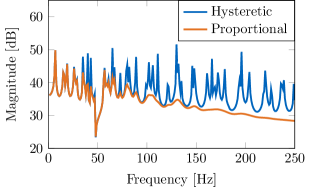
(b) Root mean square of displacement for both plates with different damping mechanisms.

Figure 1: Sketch and transfer function of the vibrating plates.

The models are reduced using all methods described in the beginning of this section, except SOBT not being applicable to the hysteretically damped model, because $\boldsymbol{\mathbf{C}}=0$ in this system. The presampling basis for minrel, avg and $\mathsf{L}_{\infty}$ considers $n_{\mathrm{s}}=250$ frequency shifts distributed linearly in $2\pi\mathrm{i}[1,250]$. Since the models are described by standard second-order transfer functions, sp yields 3 columns for each interpolation point. Using $n_{\mathrm{s}}=80$ shifts linearly distributed in the same range and augmented by shifts at $2\pi\mathrm{i}[46,47,48,50]$ yields the intermediate reduction basis with $q=250$. The additional shifts are introduced to capture the local behavior near the tuning frequency of the TVAs. A local order of $10$ is chosen for soa presampling. The intermediate basis of order $q=250$ is computed considering $n_{\mathrm{s}}=21$ shifts linearly distributed in $2\pi\mathrm{i}[1,250]$ and four additional shifts at $2\pi\mathrm{i}[46,47,48,50]$. The expansion point sampling for equi is modified similarly to the presampling methods to account for the high impact of the TVAs on the transfer function near their tuning frequency. The shifts at $2\pi\mathrm{i}[46,47,48,49,50]$ are always considered, the location of the remaining shifts are linearly distributed in the frequency range of interest. For orders $r<5$ only the first $r$ extra shifts were considered.

graphics/hysteretic_morscore.texgraphics/externalize/hysteretic_morscore.pdf

Figure 2: MORscores of all employed reduction methods for the hysteretically damped plate, with maximum accuracy $\epsilon=$1\text{$\cdot$}{10}^{-6}$$ and maximum order $r_{\mathrm{max}}=250$.

We consider the results for the plate with hysteretic damping. Despite the high number of weakly damped poles in the transfer function, all applicable methods are able to compute reasonably accurate reduced-order models. The MORscores referenced to $\epsilon=$1\text{$\cdot$}{10}^{-6}$$ and $r_{\mathrm{max}}=250$ are given in Figure 2. The choice of the tolerance value is motivated by the fact that due to the conditioning of the example the relative approximation errors do not drop below $1\text{$\cdot$}{10}^{-3}$ for any employed method. Choosing a smaller $\epsilon$ would hinder the proper comparison of the model order reduction methods. The projections with complex-valued basis matrices yield good results for all reduction methods, only $\mathsf{L}_{\infty}$ soa falls short. It has to be noted, that all reduced models computed from a soa presampling need higher reduced orders $r$ to be as accurate as the other methods. This comes from the focus on derivatives of the transfer function in a smaller number of expansion points compared to the other methods. Employing real-valued projections yields comparable MORscores. When using $\mathsf{L}_{\infty}$ in combination with soa, the order of the reduced models is increased in steps of $10$, which is the chosen size of the second-order Krylov subspaces employed. Therefor, larger reduced models are constructed in comparison to the other methods, but less computational effort is required for the presampling process. Figure 3 shows the (approximate) relative $\mathcal{L}_{\infty}$-errors plotted over the reduced order. It can be seen that all methods including $\mathsf{L}_{\infty}$ soa are able to compute reduced models of the same accuracy given a large enough reduced order.

graphics/hysteretic_err_hinf.texgraphics/externalize/hysteretic_err_hinf.pdf

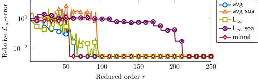
Figure 3: Relative $\mathcal{L}_{\infty}$-error for reduced models of the plate model with hysteretic damping computed by several reduction methods and osimaginput projection.

Now, we consider the results for the proportionally damped plate model. The reduction methods yield models with on overall better accuracy compared to the model with hysteretic damping, as there are less weakly damped poles in the transfer function. Because of this, the accuracy for computing the MORscore is set to $\epsilon=$1\text{$\cdot$}{10}^{-16}$$; again, we consider $r_{\mathrm{max}}=250$. The MORscores for all employed methods are given in Figure 4. Especially avg, $\mathsf{L}_{\infty}$ and minrel using the standard presampling method have high MORscores, while the models obtained from methods considering soa or sp presampling have slightly lower MORscores. This is acceptable considering the lower computational cost for computing these presampling bases, especially for soa. Only $\mathsf{L}_{\infty}$ soa has a considerably lower MORscore. It can be seen in the error-per-order plot Figure 5 that the reduced model computed by $\mathsf{L}_{\infty}$ soa reaches the error level of the other methods for a reduced order $r=250$. Its lower MORscore is mainly influenced by the fact that the reduced order $r$ is again incremented in steps of $10$, i.e., the size of the employed Krylov subspace. We can also observe that the presampling methods have a comparable influence on avg, $\mathsf{L}_{\infty}$ and minrel. Using the standard presampling, the best achievable accuracy can be reached with reduced models of order around $r=60$, models computed from sp presampling require $r=90$, and using soa yields comparable accuracy for reduced models larger than $r=100$. $\mathsf{L}_{\infty}$ soa requires a larger reduced order $r$, because $r$ is a multiple of 10 here. However, avg and minrel in combination with soa are comparable to equi. Thus, the presampling subspace computed by soa is able to capture the most important features of the original system’s transfer function. The reduced models computed with the one-sided SOBT do not reach the accuracy of the other methods and attain their best approximation error around $r\geq 160$.

graphics/rayleigh_morscore.texgraphics/externalize/rayleigh_morscore.pdf

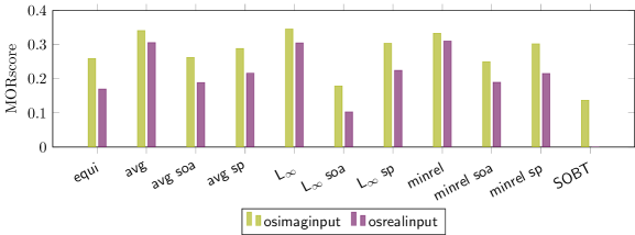
Figure 4: MORscores of all employed reduction for the proportionally damped plate, with maximum accuracy $\epsilon=$1\text{$\cdot$}{10}^{-16}$$ and maximum order $r_{\mathrm{max}}=250$.

graphics/rayleigh_err_hinf.texgraphics/externalize/rayleigh_err_hinf.pdf

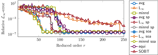
Figure 5: Relative $\mathcal{L}_{\infty}$-errors of reduced models of the plate model with proportional damping computed by several reduction methods with osimaginput projection.

The reason for the stagnation of the approximation error of reduced models computed by $\mathsf{L}_{\infty}$ soa can be observed in the transfer function error plot Figure 6. The relatively high error in the frequency region near the tuning frequency of the TVA at $f=$48\text{\,}\mathrm{Hz}$$ is present up to models with $r=240$. Only at $r=250$, $\mathsf{L}_{\infty}$ selects the shift and corresponding subspace providing enough information to approximate the original transfer function also in this frequency region. Thus, the error drops to the level of the models computed using the other reduction methods.

graphics/rayleigh_tf_red.texgraphics/externalize/rayleigh_tf_red.pdf

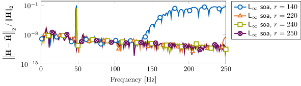
Figure 6: Pointwise relative transfer function errors for reduced-order models of the proportionally damped plate computed by $\mathsf{L}_{\infty}$ soa. The error peak near the tuning frequency of the TVAs at $f=$48\text{\,}\mathrm{Hz}$$ is clearly visible for reduced-order models of size $r<250$.

In order to compare the different formulas for SOBT given in Table 1, a slightly modified model of the proportionally damped plate is considered in the following. Here, the displacement is evaluated at the load location rather than averaged over the plate’s surface. The resulting SISO system allows the computation of a left projection basis $\boldsymbol{\mathbf{W}}$ in reasonable time. The transfer function of the resulting systems, of the computed reduced-order models using SOBT as well as the relative approximation errors are shown in Figure 7. All formulas, except vpm pm which fail at computing reduced-order models approximating the original transfer function, yield reasonably accurate reduced models. Similar to the results above, the very local effect of the TVAs around $f=$48\text{\,}\mathrm{Hz}$$ cannot easily be captured by the reduction method, resulting in a visible peak in the relative error in this frequency region even for a reduced order of $r=250$.

graphics/rayleigh_single_tf_red.texgraphics/externalize/rayleigh_single_tf_red.pdf

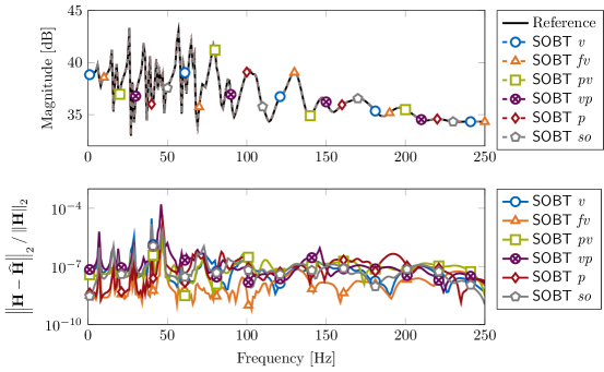
Figure 7: Comparison of the SOBT formulas. Original and reduced transfer functions as well as relative errors for the proportionally damped plate with a single output and reduced order $r=250$. Note the approximation error maximum around the tuning frequency of the TVA ($f=$48\text{\,}\mathrm{Hz}$$).

The MORscores of all other methods employed to compute reduced models for the single output version of the example are shown in Figure 8. The results are similar to the ones reported above and all methods produce accurate reduced models. Again, $\mathsf{L}_{\infty}$ soa has a lower MORscore, as the $r$ is incremented in steps of $k=10$. All reduced-order models capture the transfer function in the critical region around $f=$48\text{\,}\mathrm{Hz}$$ for large enough reduced orders. As the displacement at the loading point is evaluated in the transfer function, i.e., input and output vectors are identical such that a two-sided projection is not beneficial and tsimag, osimaginput and osimagoutput show nearly the same MORscores. The same holds for the real-valued projections. We note that avg and minrel with classical presampling yield nearly identical results for complex- and real-valued truncation matrices.

graphics/rayleigh_single_morscore.texgraphics/externalize/rayleigh_single_morscore.pdf

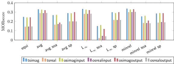
Figure 8: MORscores of all employed reduction for the proportionally damped plate with a single output, using the maximum accuracy $\epsilon=$1\text{$\cdot$}{10}^{-16}$$ and maximum order $r_{\mathrm{max}}=250$.

4.3 Sound transmission through a plate

Radiation of vibrating plates and excitation of a structure by an oscillating acoustic fluid are modeled in this example. The system consists of a cuboid acoustic cavity, where one wall is considered a system of two parallel elastic brass plates with a $2\text{\,}\mathrm{cm}$ air gap between them; all other walls are considered rigid. The plates measure $0.2\times$0.2\text{\,}\mathrm{m}$$ and have a thickness of $t=$0.9144\text{\,}\mathrm{mm}$$. The material parameters $E=$104\text{\,}\mathrm{GPa}$$, $\rho=$8500\text{\,}\mathrm{kg}\text{\,}{\mathrm{m}}^{-3}$$ $\nu=$0.37$$ are considered for brass. The receiving cavity is $0.2\text{\,}\mathrm{m}$ wide; wave speed $c=$343\text{\,}\mathrm{m}\text{\,}{\mathrm{s}}^{-1}$$ and density $\rho=$1.21\text{\,}\mathrm{kg}\text{\,}{\mathrm{m}}^{-3}$$ are considered for the acoustic fluid. The configuration is based on an experiment conducted in [33]. It is sketched in Figure 9(a) along with the acoustic pressure in the cavity resulting from a uniform pressure load $p$ applied to the outer plate. The pressure is measured at the middle point of the wall opposite to the elastic plate $P_{1}$. Energy dissipation inside the structural part of the system is modeled using proportional damping with $\beta=$1\text{$\cdot$}{10}^{-7}$$. The system is discretized using the finite element method and $n=$95\,480$$ degrees of freedom are required to obtain an accurate result in a frequency range up to $1000\text{\,}\mathrm{Hz}$. No acoustic sources are present, so the excitation vector is frequency independent. Considering the two way coupling between structure and fluid leads to non-symmetric system matrices. Thus, a transfer function of Case A with real-valued matrices is used to describe the system.

(a) Sketch of the problem with pressure load $p$ and evaluation point $P_{1}$.

graphics/guy_damped.texgraphics/externalize/guy_damped.pdf

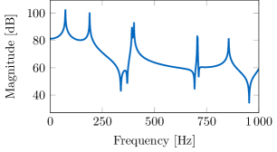
(b) Transfer function.

Figure 9: Sketch and transfer function of the sound transmission problem.

The standard presampling for minrel, avg and $\mathsf{L}_{\infty}$ considers $n_{\mathrm{s}}=200$ frequency shifts distributed linearly in $2\pi\mathrm{i}[1,1000]$. As the quadratic frequency associated with the mass matrix is the highest order of $s$ in the transfer function, each shift computed by a sp presampling contributes three columns to the intermediate basis. Therefor, $n_{\mathrm{s}}=67$ shifts, linearly distributed in the same range, are chosen such that the intermediate reduction basis is of size $q=201$. For soa, a local order $k=10$ along with $n_{\mathrm{s}}=20$ is chosen, yielding an intermediate reduction basis of order $q=200$. Because the numerical model contains unstable eigenvalues, the required Gramians for SOBT cannot be computed and, thus, the method is not applied.

graphics/guy_morscore.texgraphics/externalize/guy_morscore.pdf

Figure 10: MORscores of all employed reduction and projection methods for the sound transmission problem, with maximum accuracy $\epsilon=$1\text{$\cdot$}{10}^{-16}$$ and maximum order $r_{\mathrm{max}}=100$.

The MORscores given in Figure 10 show that especially the two-sided projections yield very good results with the highest MORscores observed. As expected, $\mathsf{L}_{\infty}$ soa falls short due to the reduced order being again incremented in steps of $10$. But also avg soa and minrel soa perform not as good as the other methods, while still showing a MORscore larger than $0.3$, which is comparable to the other numerical examples. It can be seen that using one-sided projections has a significant impact on the approximation quality. The error comparisons in Figure 11 show that the approximation error of the one-sided projections stagnates at around $1\text{$\cdot$}{10}^{-5}$, while the two-sided projections yield models with higher accuracy. As expected, the real-valued projection yield reduced-order models of comparable accuracy for higher $r$.

graphics/guy_err_hinf.texgraphics/externalize/guy_err_hinf.pdf

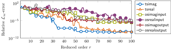
Figure 11: Comparison of the relative $\mathcal{L}_{\infty}$-errors of reduced models of the sound transmission problem computed with equi using different projections.

4.4 Radiation and scattering of a complex geometry

Now, we consider a complex geometry based on a rigid block with various openings, cavities and sharp corners. The experiment introduced in [36] is called ?radiatterer? as both radiation and scattering effects are taken into account. The basic shape is a box with dimensions $2.5\times 2.0\times$1.7\text{\,}\mathrm{m}$$, which is enclosed by an acoustic fluid of size $3.5\times 3.0\times$2.7\text{\,}\mathrm{m}$$. The geometry is sketched in Figure 12(a); for the exact shape, see [36]. A normal velocity $v_{\mathrm{n}}=$0.001\text{\,}\mathrm{m}\text{\,}{\mathrm{s}}^{-1}$$ acts on the complete surface of the geometry and excites the surrounding acoustic fluid. The free radiation from the geometry is realized with a PML of thickness $d=$0.3\text{\,}\mathrm{m}$$. It is tuned to $f=$500\text{\,}\mathrm{Hz}$$ to eliminate the frequency dependency of the PML matrices [55]. Thus, this system is described by a transfer function of Case B with complex symmetric matrices and a frequency-dependent excitation vector. The numerical model has an order of $n=$250\,000$$ and is evaluated in a frequency range from 1 to $600\text{\,}\mathrm{Hz}$. The transfer function plotted in Figure 12(b) measures the sound pressure level at a point inside the large cutout at $(x,y,z)=(0.6,0.5,0.8)$\mathrm{m}$$. A reference solution is available in [41], where the same problem has been analyzed using a boundary element method.

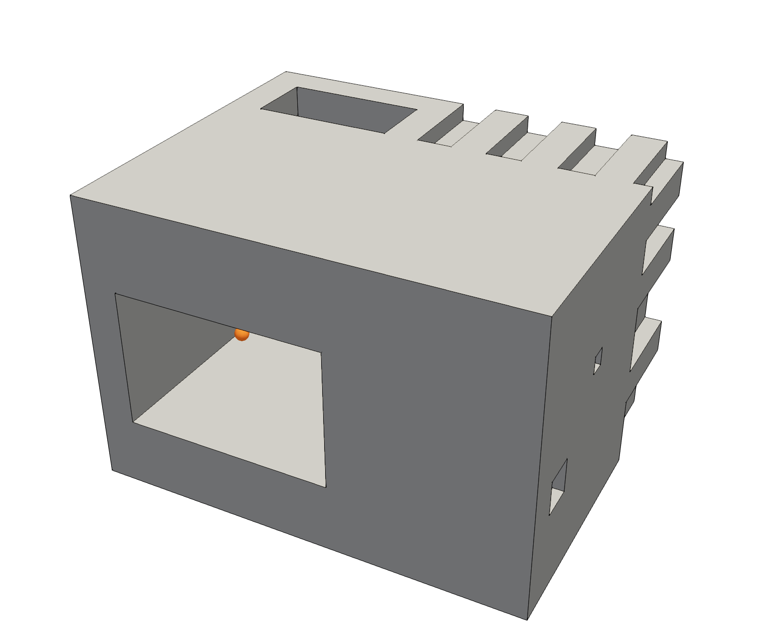
(a) Geometry sketch and probe location $P_{5}$ (orange ball).

graphics/radiatterer_p5.texgraphics/externalize/radiatterer_p5.pdf

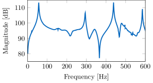
(b) Sound pressure level at $P_{5}$.

Figure 12: Sketch and transfer function of the radiation problem.

The standard presampling considers $n_{\mathrm{s}}=200$ frequency shifts distributed linearly in $2\pi\mathrm{i}\left[1,600\right]$. Again, sp yields three columns for the intermediate reduction basis, i.e., $n_{\mathrm{s}}=67$ linearly distributed shifts are chosen to obtain a basis of size $q=201$. For soa, a local order $k=5$ is used such that $n_{\mathrm{s}}=40$ expansion points yield a presampling basis with order $q=200$. A lower local order is chosen for this model as many weakly damped modes are present in the transfer function and otherwise not enough information about the full-order model would be available in the intermediate reduction basis. SOBT is not applicable to this problem because of its frequency-dependent input vector.

graphics/radiatterer_morscore.texgraphics/externalize/radiatterer_morscore.pdf

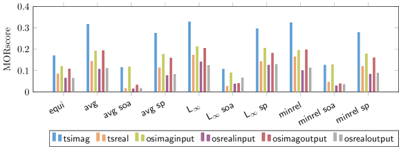
Figure 13: MORscores of all employed reduction for the scattering problem, with the maximum accuracy $\epsilon=$1\text{$\cdot$}{10}^{-16}$$ and maximum order $r_{\mathrm{max}}=200$.

The MORscores for each applied reduction method are given in Figure 13. It can be seen that again two-sided interpolation with complex-valued bases outperforms the other projection methods. The lower rate of approximation when using presampling based on soa is also in line with the observations from the previous experiments. equi shows also a considerably worse performance than the methods based on presampling. It can be seen in the error-per-order plot Figure 14 that the error of reduced-order models computed with equi stagnates until approximately $r=140$ before it drops to the same level as the other methods. This suggests that important features of the system response have not been captured by the smaller reduction bases. The oscillating behavior of the relative error in the region of $150<r<190$ is a sign that crucial parts of the transfer function are missed by sampling with equidistantly distributed expansion points.

graphics/radiatterer_new_err_hinf.texgraphics/externalize/radiatterer_new_err_hinf.pdf

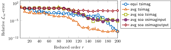
Figure 14: Relative $\mathcal{L}_{\infty}$-errors of reduced models of the radiation problem computed by several reduction methods.

These observations are supported by Figure 15 plotting the relative errors of reduced-order models computed by equi with orders $r=140$ and $r=200$. While the larger reduced-order model shows a very small error over the complete frequency range, the smaller does not for the frequency region above $450\text{\,}\mathrm{Hz}$. It is, however, also apparent, that the approximation quality for all methods is better in the lower frequency range, presumably because of a large number of modes in the region above $450\text{\,}\mathrm{Hz}$. If this is known a priori, the locations of the expansion points can be altered appropriately. If this is not possible, the presampling involved in the methods avg, $\mathsf{L}_{\infty}$ and minrel shows its benefit. At the cost of computing a larger intermediate reduction basis, the most relevant information from this basis is chosen, allowing smaller reduced models with better accuracy. Choosing standard presampling or sp presampling yields accurate reduced-order models with acceptable high MORscores.

If soa presampling is employed, the resulting reduced-order models are less accurate than using the other presampling methods. For some projections, the reduced-order models do not accurately approximate the original transfer function, cf. Figure 14. The error graph for avg soa tsimag in Figure 15 shows characteristic spikes at the locations of the expansion points in the presampling basis. This suggests that the employed second-order Krylov subspace does not contain enough information to enable an as accurate approximation as the other presampling methods. A remedy would be to increase the size of the Krylov space, which would in turn increase the size of the presampling basis. Note that increasing the size of the Krylov space is up to a certain degree less computationally expensive than establishing a completely new shift. Projection regarding the system output using a soa presampling, however, does not yield a good approximation of the original system at all.

graphics/radiatterer_tf_red.texgraphics/externalize/radiatterer_tf_red.pdf

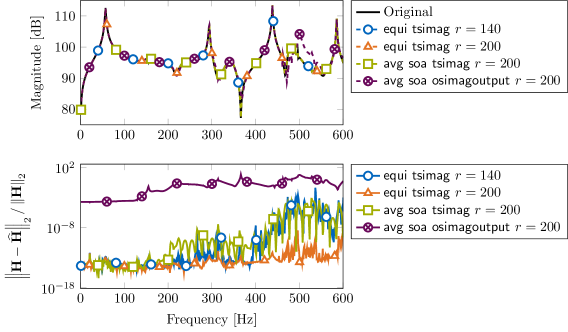
Figure 15: Original and reduced transfer functions as well as relative errors for the radiation problem reduced with different methods.

4.5 Acoustic cavity with poroelastic layer

An acoustic cavity with dimensions $0.75\times 0.6\times$0.4\text{\,}\mathrm{m}$$ is examined in the following example. One wall is covered by a $0.05\text{\,}\mathrm{m}$ thick poroelastic layer acting as a sound absorber. The poroelastic material is described by the Biot theory [17]. The system is excited by an acoustic point source located in the corner opposite to the porous material. A sketch of the system is given in 16(a). The geometry and material parameters are taken from [49], and the discretized finite element model has the order $n=$386\,076$$. We evaluate the model in the frequency range $100\text{\,}\mathrm{Hz}1000\text{\,}\mathrm{Hz}$. The material’s frequency dependent dissipation mechanism and the coupling between solid and fluid phase inside the material are modeled with in total six complex-valued functions. Due to the acoustic source, the transfer function also has a frequency-dependent input vector. Thus, the system can be described by a Case C transfer function with non-symmetric and complex-valued system matrices. The transfer function measures the sound pressure level averaged over the acoustic domain and is given in Figure 16(b).

(a) Sketch of the poroacoustic system with acoustic point source $q$. The porous material covers the right wall.

graphics/rumpler2014.texgraphics/externalize/rumpler2014.pdf

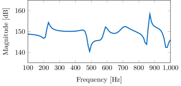
(b) Mean sound pressure level in the acoustic domain.

Figure 16: Sketch and transfer function of the poroacoustic model.

The model is reduced using all methods except SOBT, which is not applicable to this system because of the transfer function structure. The standard presampling for minrel, avgand $\mathsf{L}_{\infty}$ considers $n_{\mathrm{s}}=200$ frequency shifts distributed linearly in $2\pi\mathrm{i}[100,1000]$. The analytic derivatives of the frequency-dependent functions vanish for orders larger than $6$ in the considered frequency range such that sp yields 7 columns for each shift. Using $n_{\mathrm{s}}=29$ shifts linearly distributed in the same range yields the corresponding intermediate reduction basis with $q=203$. For soa presampling, a local order of $10$ is chosen for each of the $n_{\mathrm{s}}=20$ shifts, which are also linearly distributed in $2\pi\mathrm{i}[100,1000]$. This results in an intermediate reduction basis of order $q=200$.

graphics/rumpler_morscore.texgraphics/externalize/rumpler_morscore.pdf

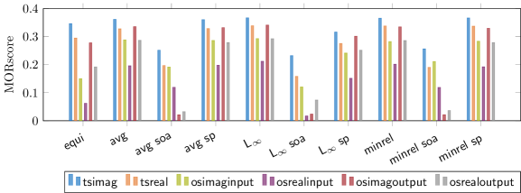
Figure 17: MORscores of all employed reduction methods for the poroacoustic system, with the maximum accuracy $\epsilon=$1\text{$\cdot$}{10}^{-16}$$ and maximum order $r_{\mathrm{max}}=100$.

The MORscores of employed methods are reported in Figure 17 and show a good performance of nearly all reduction methods. Even $\mathsf{L}_{\infty}$ sp, whose reduced-order models are incremented in steps of $r=7$ has a comparable MORscore. Additionally, it reaches an error as low as the other good performing methods around $r=28$, cf. Figure 18. As already observed, the projections considering only the system output yield worse results if used in combination with soa presampling. To use soa for this experiment, the approximations of the nonlinear frequency-dependent functions are truncated after the quadratic term so that the second-order Krylov subspace can be used. This has an impact on the approximation quality of the reduced-order models and results in a slower convergence of the approximation errors compared to the other presampling strategies. However, a comparably small error can also be achieved with soa, if $r$ is chosen high enough. Figure 18 compares the approximated relative $\mathcal{L}_{\infty}$-errors over the reduced order for the different presampling methods. The good performance of sp is evident here. It is also interesting to note, that an osimagoutput projection yields models, which accuracy is comparable to tsreal for all methods except soa.

graphics/rumpler_err_hinf.texgraphics/externalize/rumpler_err_hinf.pdf

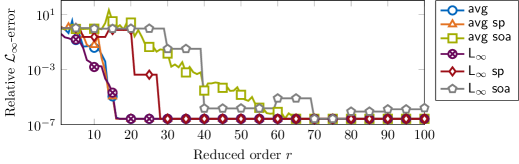
Figure 18: Relative $\mathcal{L}_{\infty}$-errors of reduced models of the poroacoustic system computed by several reduction methods. A two-sided projection with complex-valued bases is considered for all cases.

5 Conclusions

In this work, we described structure-preserving model order reduction methods based on rational interpolation and balanced truncation applied to models of vibro-acoustic systems. The benchmark examples were chosen such that their transfer functions exhibit different properties, for example, complex-valued and/or frequency-dependent system matrices or a frequency-dependent excitation. Each benchmark case represents a relevant class of vibro-acoustic problems. We also presented a strategy to incorporate higher-order frequency-dependent terms in a standard second-order reduction framework.

The interpolation-based methods have been applicable to all considered models and have been able to compute reduced-order models of reasonable accuracy and small size. Second-order balanced truncation also has succeeded in computing compact reduced models. However, it is not applicable to systems with non-standard second-order transfer functions, which strongly restricts its application to vibro-acoustic systems. The methods based on oversampling the frequency response and extracting the most relevant information have been shown to be the most successful. Strategies to leverage the initial cost of computing the presampling data have been proposed and showed in many cases comparable results.

References

- [1] N. Aliyev, P. Benner, E. Mengi, and M. Voigt. A subspace framework for -norm minimization. SIAM J. Matrix Anal. Appl., 41(2):928–956, 2020. doi:10.1137/19M125892X.
- [2] K. Amichi and N. Atalla. A new 3D finite element for sandwich beams with a viscoelastic core. J. Vib. Acoust., 131(2):021010, 2009. doi:10.1115/1.3025828.
- [3] A. C. Antoulas, C. A. Beattie, and S. Gugercin. Interpolatory Methods for Model Reduction. Computational Science & Engineering. SIAM, Philadelphia, PA, 2020. doi:10.1137/1.9781611976083.
- [4] R. J. Astley. Infinite elements. In S. Marburg and B. Nolte, editors, Computational Acoustics of Noise Propagation in Fluids - Finite and Boundary Element Methods, pages 197–230. Springer, Berlin, Heidelberg, 2008. doi:10.1007/978-3-540-77448-8_8.
- [5] Z. Bai and Y. Su. Dimension reduction of large-scale second-order dynamical systems via a second-order Arnoldi method. SIAM J. Sci. Comput., 26(5):1692–1709, 2005. doi:10.1137/040605552.
- [6] Z. Bai and Y. Su. SOAR: A second-order Arnoldi method for the solution of the quadratic eigenvalue problem. SIAM J. Matrix Anal. Appl., 26(3):640–659, 2005. doi:10.1137/S0895479803438523.
- [7] G. A. Baker Jr. Essentials of Padé Approximants. Academic Press, New York, 1975.
- [8] C. A. Beattie and S. Gugercin. Interpolatory projection methods for structure-preserving model reduction. Syst. Control Lett., 58(3):225–232, 2009. doi:10.1016/j.sysconle.2008.10.016.
- [9] C. A. Beattie and S. Gugercin. Realization-independent -approximation. In 51st IEEE Conference on Decision and Control (CDC), pages 4953–4958, 2012. doi:10.1109/CDC.2012.6426344.
- [10] R. S. Beddig, P. Benner, I. Dorschky, T. Reis, P. Schwerdtner, M. Voigt, and S. W. R. Werner. Structure-preserving model reduction for dissipative mechanical systems. e-print 2010.06331, arXiv, 2020. math.OC. URL: https://arxiv.org/abs/2010.06331.
- [11] P. Benner, P. Goyal, and I. Pontes Duff. Identification of dominant subspaces for linear structured parametric systems and model reduction. e-print 1910.13945, arXiv, 2019. math.NA. URL: https://arxiv.org/abs/1910.139450.
- [12] P. Benner, M. Köhler, and J. Saak. Matrix equations, sparse solvers: M-M.E.S.S.-2.0.1—Philosophy, features and application for (parametric) model order reduction. In P. Benner, T. Breiten, H. Faßbender, M. Hinze, T. Stykel, and R. Zimmermann, editors, Model Reduction of Complex Dynamical Systems, volume 171 of International Series of Numerical Mathematics, pages 369–392. Birkhäuser, Cham, 2021. doi:10.1007/978-3-030-72983-7_18.
- [13] P. Benner and S. W. R. Werner. Frequency- and time-limited balanced truncation for large-scale second-order systems. Linear Algebra Appl., 623:68–103, 2021. Special issue in honor of P. Van Dooren, Edited by F. Dopico, D. Kressner, N. Mastronardi, V. Mehrmann, and R. Vandebril. doi:10.1016/j.laa.2020.06.024.
- [14] P. Benner and S. W. R. Werner. SOLBT – Limited balanced truncation for large-scale sparse second-order systems (version 3.0), April 2021. doi:10.5281/zenodo.4600763.
- [15] H. Bériot and A. Modave. An automatic perfectly matched layer for acoustic finite element simulations in convex domains of general shape. Int. J. Numer. Methods Eng., 122(5):1239–1261, 2020. doi:10.1002/nme.6560.
- [16] B. Besselink, U. Tabak, A. Lutowska, N. Van de Wouw, H. Nijmeijer, D. J. Rixen, M. E. Hochstenbach, and W. H. A. Schilders. A comparison of model reduction techniques from structural dynamics, numerical mathematics and systems and control. J. Sound Vib., 332(19):4403–4422, 2013. doi:10.1016/j.jsv.2013.03.025.
- [17] M. A. Biot. Theory of propagation of elastic waves in a fluid‐saturated porous solid. I. Low‐frequency range. J. Acoust. Soc. Am., 28(2):168–178, 1956. doi:10.1121/1.1908239.
- [18] A. Bultheel and M. Van Barel. Padé techniques for model reduction in linear system theory: a survey. J. Comput. Appl. Math., 14(3):401–438, 1986. doi:10.1016/0377-0427(86)90076-2.
- [19] Y. Chahlaoui, D. Lemonnier, A. Vandendorpe, and P. Van Dooren. Second-order balanced truncation. Linear Algebra Appl., 415(2–3):373–384, 2006. doi:10.1016/j.laa.2004.03.032.
- [20] C.-C. Chu, H.-C. Tsai, and M.-H. Lai. Structure preserving model-order reductions of MIMO second-order systems using Arnoldi methods. Math. Comput. Model., 51(7–8):956–973, 2010. doi:10.1016/j.mcm.2009.08.028.
- [21] C. Claeys, E. Deckers, and W. D. Pluymers. A lightweight vibro-acoustic metamaterial demonstrator: Numerical and experimental investigation. Mech. Syst. Signal Process., 70–71:853–880, 2016. doi:10.1016/j.ymssp.2015.08.029.
- [22] C. C. Claeys, K. Vergote, P. Sas, and W. Desmet. On the potential of tuned resonators to obtain low-frequency vibrational stop bands in periodic panels. J. Sound Vib., 332(6):1418–1436, 2013. doi:10.1016/j.jsv.2012.09.047.
- [23] P. Dadvand, R. Rossi, and E. Oñate. An object-oriented environment for developing finite element codes for multi-disciplinary applications. Arch. Comput. Methods Eng., 17(3):253–297, 2010. doi:10.1007/s11831-010-9045-2.
- [24] C. De Villemagne and R. E. Skelton. Model reductions using a projection formulation. Internat. J. Control, 46(6):2141–2169, 1987. doi:10.1080/00207178708934040.
- [25] E. Deckers, W. Desmet, K. Meerbergen, and F. Naets. Case studies of model order reduction for acoustics and vibrations. In P. Benner, A. Grivet-Talocia, S. Quarteroni, G. Rozza, W. Schilders, and L. M. Silveira, editors, Model Order Reduction – Volume 3: Applications, pages 75–110. De Gruyter, 2020. doi:10.1515/9783110499001-003.
- [26] F. Duddeck. Multidisciplinary optimization of car bodies. Struct. Multidiscip. Optim., 35(4):375–389, 2008. doi:10.1007/s00158-007-0130-6.
- [27] L. Feng and P. Benner. A new error estimator for reduced-order modeling of linear parametric systems. IEEE Trans. Microw. Theory Tech., 67(12):4848–4859, 2019. doi:10.1109/TMTT.2019.2948858.
- [28] V. M. Ferrándiz, P. Bucher, R. Rossi, R. Zorrilla, J. Cotela, J. Maria, M. A. Celigueta, and G. Casas. KratosMultiphysics/Kratos: KratosMultiphysics 8.1, November 2020. doi:10.5281/zenodo.4289897.
- [29] D. Givoli. Recent advances in the DtN FE method. Arch. Comput. Methods Eng., 6(2):71–116, 1999. doi:10.1007/BF02736182.
- [30] W. B. Gragg and A. Lindquist. On the partial realization problem. Linear Algebra Appl., 50:277–319, 1983. doi:10.1016/0024-3795(83)90059-9.
- [31] E. J. Grimme. Krylov projection methods for model reduction. PhD thesis, University of Illinois, Urbana-Champaign, USA, 1997. URL: https://perso.uclouvain.be/paul.vandooren/ThesisGrimme.pdf.
- [32] S. Gugercin, A. C. Antoulas, and C. Beattie. model reduction for large-scale linear dynamical systems. SIAM J. Matrix Anal. Appl., 30(2):609–638, 2008. doi:10.1137/060666123.
- [33] R. W. Guy. The transmission of airborne sound through a finite panel, air gap, panel and cavity configuration – a steady state analysis. Acta Acust. united Acust., 49(4):323–333, 1981.
- [34] U. Hetmaniuk, R. Tezaur, and C. Farhat. Review and assessment of interpolatory model order reduction methods for frequency response structural dynamics and acoustics problems. Int. J. Numer. Methods Eng., 90(13):1636–1662, 2012. doi:10.1002/nme.4271.
- [35] C. Himpe. Comparing (empirical-Gramian-based) model order reduction algorithms. In P. Benner, T. Breiten, H. Faßbender, M. Hinze, T. Stykel, and R. Zimmermann, editors, Model Reduction of Complex Dynamical Systems, volume 171 of International Series of Numerical Mathematics, pages 141–164. Birkhäuser, Cham, 2021. doi:10.1007/978-3-030-72983-7_7.
- [36] M. Hornikx, M. Kaltenbacher, and S. Marburg. A platform for benchmark cases in computational acoustics. Acta Acust. united Acust., 101(4):811–820, 2015. doi:10.3813/AAA.918875.
- [37] F. Ihlenburg. Finite Element Analysis of Acoustic Scattering, volume 132 of Appl. Math. Sci. Springer, New York, NY, 1998. doi:10.1007/b98828.
- [38] P. Lietaert, K. Meerbergen, J. Pérez, and B. Vandereycken. Automatic rational approximation and linearization of nonlinear eigenvalue problems. IMA J. Numer. Anal., 00:1–29, 2021. doi:10.1093/imanum/draa098.
- [39] D. Lu, Y. Su, and Z. Bai. Stability analysis of the two-level orthogonal Arnoldi procedure. SIAM J. Matrix Anal. Appl., 37(1):195–214, 2016. doi:10.1137/151005142.
- [40] S. Marburg. Developments in structural-acoustic optimization for passive noise control. Arch. Comput. Methods Eng., 9(4):291–370, 2002. doi:10.1007/BF03041465.
- [41] S. Marburg. The Burton and Miller method: Unlocking another mystery of its coupling parameter. J. Comput. Acoust., 24(1):1550016, 2016. doi:10.1142/S0218396X15500162.
- [42] A. T. Mathis, N. N. Balaji, R. J. Kuether, A. R. Brink, M. R. W. Brake, and D. D. Quinn. A review of damping models for structures with mechanical joints. Appl. Mech. Rev., 72(4):040802, 2020. doi:10.1115/1.4047707.
- [43] D. G. Meyer and S. Srinivasan. Balancing and model reduction for second-order form linear systems. IEEE Trans. Autom. Control, 41(11):1632–1644, 1996. doi:10.1109/9.544000.
- [44] B. C. Moore. Principal component analysis in linear systems: controllability, observability, and model reduction. IEEE Trans. Autom. Control, AC–26(1):17–32, 1981. doi:10.1109/TAC.1981.1102568.
- [45] Y. Nakatsukasa, O. Sète, and L. N. Trefethen. The AAA algorithm for rational approximation. SIAM J. Sci. Comput., 40(3):A1494–A1522, 2018. doi:10.1137/16M1106122.
- [46] T. Reis and T. Stykel. Balanced truncation model reduction of second-order systems. Math. Comput. Model. Dyn. Syst., 14(5):391–406, 2008. doi:10.1080/13873950701844170.
- [47] L. Rouleau, J.-F. Deü, and A. Legay. A comparison of model reduction techniques based on modal projection for structures with frequency-dependent damping. Mech. Syst. Signal Process., 90:110–125, 2017. doi:10.1016/j.ymssp.2016.12.013.
- [48] R. Rumpler. Padé approximants and the modal connection: Towards increased robustness for fast parametric sweeps. Int. J. Numer. Methods Eng., 113(1):65–81, 2018. doi:10.1002/nme.5603.
- [49] R. Rumpler, P. Göransson, and J.-F. Deü. A finite element approach combining a reduced‐order system, Padé approximants, and an adaptive frequency windowing for fast multi‐frequency solution of poro‐acoustic problems. Int. J. Numer. Methods Eng., 97(10):759–784, 2014. doi:10.1002/nme.4609.
- [50] J. Saak, M. Köhler, and P. Benner. M-M.E.S.S. – The Matrix Equations Sparse Solvers library (version 2.0.1), February 2020. see also: https://www.mpi-magdeburg.mpg.de/projects/mess. doi:10.5281/zenodo.3606345.
- [51] J. Saak, D. Siebelts, and S. W. R. Werner. A comparison of second-order model order reduction methods for an artificial fishtail. at-Automatisierungstechnik, 67(8):648–667, 2019. doi:10.1515/auto-2019-0027.
- [52] P. Schwerdtner and M. Voigt. Computation of the -norm using rational interpolation. IFAC-PapersOnLine, 51(25):84–89, 2018. 9th IFAC Symposium on Robust Control Design ROCOND 2018, Florianópolis, Brazil. doi:10.1016/j.ifacol.2018.11.086.
- [53] T.-J. Su and R. R. Craig Jr. Model reduction and control of flexible structures using Krylov vectors. J. Guid. Control Dyn., 14(2):260–267, 1991. doi:10.2514/3.20636.
- [54] S. Van Ophem, O. Atak, E. Deckers, and W. Desmet. Stable model order reduction for time-domain exterior vibro-acoustic finite element simulations. Comput. Methods Appl. Mech. Eng., 325:240–264, 2017. doi:10.1016/j.cma.2017.06.022.
- [55] A. Vermeil de Conchard, H. Mao, and R. Rumpler. A perfectly matched layer formulation adapted for fast frequency sweeps of exterior acoustics finite element models. J. Comput. Phys., 398:108878, 2019. doi:10.1016/j.jcp.2019.108878.
- [56] S. W. R. Werner. Structure-Preserving Model Reduction for Mechanical Systems. Dissertation, Department of Mathematics, Otto von Guericke University, Magdeburg, Germany, 2021. doi:10.25673/38617.
- [57] S. Wyatt. Issues in Interpolatory Model Reduction: Inexact Solves, Second-order Systems and DAEs. PhD thesis, Virginia Polytechnic Institute and State University, Blacksburg, Virginia, USA, 2012. URL: http://hdl.handle.net/10919/27668.
- [58] X. Xie, H. Zheng, S. Jonckheere, and W. Desmet. Explicit and efficient topology optimization of frequency-dependent damping patches using moving morphable components and reduced-order models. Comput. Methods Appl. Mech. Eng., 355:591–613, 2019. doi:10.1016/j.ymssp.2016.12.013.
- [59] X. Xie, H. Zheng, S. Jonckheere, and W. Desmet. Acoustic simulation of cavities with porous materials using an adaptive model order reduction technique. J. Sound Vib., 485:115570, 2020. doi:10.1016/j.jsv.2020.115570.