Gaussian elimination versus greedy methods for the synthesis of linear reversible circuits

Abstract

Linear reversible circuits represent a subclass of reversible circuits with many applications in quantum computing. These circuits can be efficiently simulated by classical computers and their size is polynomially bounded by the number of qubits, making them a good candidate to deploy efficient methods to reduce computational costs. We propose a new algorithm for synthesizing any linear reversible operator by using an optimized version of the Gaussian elimination algorithm coupled with a tuned LU factorization. We also improve the scalability of purely greedy methods. Overall, on random operators, our algorithms improve the state-of-the-art methods for specific ranges of problem sizes: the custom Gaussian elimination algorithm provides the best results for large problem sizes ($n>150$) while the purely greedy methods provide quasi optimal results when $n<30$. On a benchmark of reversible functions, we manage to significantly reduce the CNOT count and the depth of the circuit while keeping other metrics of importance (T-count, T-depth) as low as possible.

1 Introduction

Progress in scientific computing in recent decades is as much about improvements in algorithms as the increasing power of hardware. Some very active fields, such as machine learning, have benefited from the considerable increase in the amount of data available and from the ever more efficient hardware capable of processing this data, whereas the first algorithms were invented well before. This exponential increase in the power of our computers is often illustrated, now for 40 years, by Moore’s second law [34], that predicts that the number of transistors in microprocessors doubles every 2 years since its formulation in 1975. Behind this law hides a race for the miniaturization of transistors. Today the transistors are only a few nanometers large, at this scale quantum effects such as the tunnel effect interfere with the proper performance of the transistors so that it becomes more and more complex to reduce their size.

New kind of computational models are developing in response to this future limitation of the so-called “conventional” or “classical” computing. We can mention biological [14, 11], photonic [21], neuromorphic [33, 45] or quantum [37] computing, booming these recent years. These new paradigms are promising because they perform the calculation at new scales and potentially overcome the limitations of classical computing. For example, in quantum computing, elementary particles are directly manipulated by exploiting their quantum properties to perform in polynomial time computations that may require an exponential amount of operations on a conventional machine [41, 16].

Our paper concerns reversible computing, i.e., boolean operations that can be “undone” because they consist in a bijection between the inputs and outputs of the system. Reversible computing is a subclass of photonic and quantum computing, which motivates its study. A consequence of the reversibility is that there is no loss of information during the calculation, resulting in lower energy consumption because no energy is dissipated at the erasure of a bit [25]. Here we study reversible circuits referred to as linear reversible circuits. These circuits have the particularity to be expressed as circuits containing only one reversible logic gate: the Controlled-Not (CNOT) gate which performs the operation NOT on a target qubit conditioned by the value of a control qubit. This class of circuits is particularly useful in quantum computing in the synthesis of stabilizer circuits: canonical forms for stabilizer circuits involving linear reversible circuits have been found and the size of stabilizer circuits is dominated by the size of reversible linear circuits [1, 29] . Stabilizer circuits are for instance used for error correction and are therefore essential for scaling up quantum computing [13], and so are linear reversible circuits by extension. Linear reversible circuits are also involved in circuits called “CNOT + T” (also called phase polynomials) whose optimization is the purpose of recent research [5, 31, 4, 17].

In the following we study the synthesis and optimization of linear reversible circuits. We are given a linear reversible operator as a Boolean matrix and we seek a quantum circuit that implements it as a series of elementary operations. Our contributions are the following :

• We propose GreedyGE: an optimized version of the Gaussian elimination algorithm for synthesizing any linear reversible operator. When we zero out the subdiagonal entries of the matrix, like in a standard Gaussian elimination, we perform the operations that minimize an ad-hoc cost function, resulting in less operations for the synthesis. We study the theoretical worst case behavior of our algorithm. Overall, our algorithm is asymptotically optimal with theoretical and practical improvements over the state-of-the-art methods [38, Algo. 1] and the syndrome decoding based method [9]. In terms of computational time our algorithm is faster than the standard Gaussian elimination algorithm.

• We propose a new way to compute the LU decomposition of a linear reversible operator. This provides us triangular operators $L$ and $U$ whose synthesis yield shorter circuits, especially when the circuit is expected to be "small enough". We will detail this notion of "small enough" later in the article. This optimization finds application in other synthesis methods relying on an LU decomposition, for instance the recent method we designed using the syndrome decoding problem [9].

• We show that cost minimization techniques are useful for finding circuits whose expected size is "small enough". We briefly review the existing algorithm and we propose our own cost function and implementation that increase the range of validity of this kind of technique.

• We provide benchmarks of our methods and compare them to state-of-the-art algorithms. First we test our algorithms on random circuits of various sizes. Overall, with GreedyGE, we can synthesize circuits with more than 150 qubits in a few seconds while giving circuits that are at least 10% smaller in average than the current state of the art. With purely greedy methods, we report quasi optimal results when $n<30$. Then we include our methods into a more general Clifford+T quantum compiler — the Tpar algorithm [5] — and we show that our algorithms are also useful in practice: on a set of reversible functions we successfully reduce the total number of CNOTs and the circuit depth while keeping other metrics of interest (T-count, T-depth) as low as possible.

The plan of this paper is the following: in Section 2 we present the basic notions and state of the art about the synthesis of linear reversible circuits. In Section 3 we describe the improved Gaussian elimination algorithm on triangular operators. In Section 4 we extend our algorithm to treat any general linear reversible operator. Notably we present optimization techniques for computing the LU decomposition. We tackle the study of purely greedy methods in Section 5. Benchmarks are given in Section 6. We conclude in Section 7.

2 Background and state of the art

2.1 Notion of linear reversible function.

Let $\mathbb{F}_{2}$ be the Galois field of two elements. A boolean function $f:\mathbb{F}_{2}^{n}\to\mathbb{F}_{2}$ is said to be linear if

$$f(x_{1}\oplus x_{2})=f(x_{1})\oplus f(x_{2})$$

for any $x_{1},x_{2}\in\mathbb{F}_{2}^{n}$ where $\oplus$ is the bitwise XOR operation. Let $e_{k}$ be the $k$-th canonical vector of $\mathbb{F}_{2}^{n}$. By linearity we can write for any $x=\sum_{k}\alpha_{k}e_{k}$ (with $\alpha_{k}\in\{0,1\}$)

$$f(x)=f\left(\sum_{k}\alpha_{k}e_{k}\right)=\sum_{k}\alpha_{k}f(e_{k})$$

and the function $f$ can be represented with a column vector $\mathbf{c}=[f(e_{1}),...,f(e_{n})]^{T}$ such that $f(x)=c^{T}x$. This expression easily extends to the $n$-inputs and $m$-outputs functions $f:\mathbb{F}_{2}^{n}\to\mathbb{F}_{2}^{m}$ where $f$ is defined by an $m\times n$ boolean matrix $A$ such that

$$f(x)=Ax.$$

In the case of reversible boolean functions we have $n=m$ and the matrix $A$ must be invertible. The application of two successive operators $A$ and $B$ is equivalent to the application of the operator product $BA$. There is a one-to-one correspondence between the linear reversible functions of arity $n$ and the invertible boolean matrices of size $n$. This was used for instance to count the number of different linear reversible functions of $n$ inputs in [38].

2.2 LU decomposition.

Given the matrix representation $A$ of a generic linear reversible operator, we can always perform an LU decomposition [12] such that there exists an upper (resp. lower) triangular matrix $U$ (resp. $L$) and a permutation matrix $P$ such that $A=PLU$. The invertibility of $A$ ensures that the diagonal elements of $L$ and $U$ are all equal to $1$. In the remainder of this paper, the term “triangular operator” stands for an operator whose corresponding matrix is either upper or lower triangular. The LU decomposition is at the core of several synthesis of general linear reversible Boolean operators: synthesizing $U$, $L$, $P$ and concatenating the circuits gives an implementation of $A$.

2.3 Synthesis of linear reversible boolean functions.

We are interested in synthesizing a linear reversible boolean function into a reversible circuit, i.e., a series of elementary reversible gates that can be executed on suitable hardware. For instance in quantum computing the CNOT gate is used for superconducting and photonic qubits and performs the following 2-arity operation:

$$\text{CNOT}(x_{1},x_{2})=(x_{1},x_{1}\oplus x_{2}).$$

The CNOT gate is a linear reversible gate. It is also universal for linear reversible circuit synthesis, i.e., any linear reversible function can be implemented by a reversible circuit containing only CNOT gates [1]. In this paper we aim at producing CNOT-based reversible circuits for any linear reversible functions.

In terms of matrices, a CNOT gate controlled by the line $j$ acting on line $i\neq j$ can be written $E_{ij}=I+e_{ij}$ where $I$ is the identity matrix and $e_{ij}$ the elementary matrix with all entries equal 0 but the entry $(i,j)$ whose value is $1$. Finding a CNOT circuit implementing an operator $A$ is therefore equivalent to finding a sequence of matrices $(E_{i_{k}j_{k}})_{1\leq i_{k},j_{k}\leq n}$ such that

$$\prod_{k=1\dots N}E_{i_{k},j_{k}}=A.$$

Using the fact that $E_{ij}^{-1}=E_{ij}$, it is more convenient to rewrite the synthesis problem as a reduction of $A$ to the identity operator $I$

$$\prod_{k=N\dots 1}E_{i_{k},j_{k}}A=I$$

because we now show that the synthesis problem can be reformulated in terms of elementary operations applied on $A$. Given a CNOT with control $j$ and target $i$ applied on an operator $A$, the updated operator $E_{ij}A$ can be deduced from $A$ with an elementary row operation:

$$r_{i}\leftarrow r_{i}\oplus r_{j},$$

writing $r_{k}$ for the $k$-th row of $A$. Therefore, if one can compute a sequence of row operations transforming $A$ into the identity operator then one can construct a circuit implementing $A$ by concatenating the CNOT gates associated to each row operation. With a standard Gaussian elimination algorithm it is always possible to reduce an invertible operator to the identity with row operations. This gives a simple proof that the CNOT gate is universal for linear reversible circuit synthesis. In some cases we will also authorize the use of column operations. A column operation $c_{j}\leftarrow c_{i}\oplus c_{j}$ is equivalent to right multiplying $A$ by $E_{ij}$. Overall by combining row and column operations we get

$$\prod_{(i_{1},j_{1})}E_{i_{1}j_{1}}\times A\times\prod_{(i_{2},j_{2})}E_{i_{2}j_{2}}=I$$

and finally

$$A=\prod_{(i_{1},j_{1})}E_{i_{1}j_{1}}\prod_{(i_{2},j_{2})}E_{i2j2}$$

so we recover a CNOT circuit for the implementation of $A$.

Thus, synthesizing a linear reversible function into a CNOT-based reversible circuit is equivalent to transforming an invertible Boolean matrix $A$ to the identity by applying elementary row and column operations. From now on we will privilege this more abstract point of view because it gives more freedom and often appears clearer for the design of algorithms. We note by $\text{Row}(i,j)$ the elementary row operation $r_{j}\leftarrow r_{i}\oplus r_{j}$ and $\text{Col}(i,j)$ the elementary column operation $c_{j}\leftarrow c_{i}\oplus c_{j}$.

We use the size of the circuit, i.e., the number of CNOT gates in it, to evaluate the quality of our synthesis. The size of the circuit gives the total number of instructions the hardware has to perform during its execution. Due to the presence of noise when executing every logical gate, it is of interest to have the shortest circuit possible. Another metric of interest is the depth of the circuit which is closely related to the number of time steps required to execute the circuit. In other words the depth of a quantum circuit gives its execution time. Given that the physical qubits are subject to the decoherence problem and that the total time available to perform a quantum algorithm is limited, it is also very important to be able to produce shallow circuits.

We now review the main algorithms designed for the synthesis of CNOT circuits.

2.4 State of the art and contributions

We distinguish algorithms that assume that all qubits are connected and algorithms that take into account a restricted connectivity between the qubits. The former usually give smaller and shallower circuits while the latter are adapted to real world hardware where row operations can be performed only between qubits that are neighbors in the hardware. Studying ideal cases with full connectivity is of interest for providing us with new solutions before transposing them to the restricted case.

Gaussian elimination based algorithm.

In the literature, the first algorithm proposed is a Gaussian elimination algorithm that produces circuits of size $\mathcal{O}(n^{2})$ gates [1]. Later a lower bound of $\mathcal{O}(n^{2}/\log_{2}(n))$ was established in [38] for the asymptotic optimal size of reversible circuits, with an algorithm that reaches this lower bound. The algorithm consists in performing the Gaussian elimination algorithm on a chunk of $m$ columns. The gain in the number of operations arises when two words in $F_{2}^{m}$ are equal and that one can be zeroed in one row operation. Choosing $m=\mathcal{O}(\log_{2}(n))$ leads to an optimal asymptotic complexity.

Syndrome decoding based algorithm

Recently, we proposed a new method for the synthesis of CNOT circuits [9]. We transformed the synthesis problem into a series of syndrome decoding problems and gave several strategies to solve them (either optimal with an integer programming solver or approximate with greedy methods). Our benchmarks reveal that our method outperforms [38, Algo. 1] for operators on medium-sized registers ($n<400$ qubits) but performs poorly as $n$ gets larger.

Other algorithms.

In [40] a cost-minimization approach was used with promising results.

To our knowledge, [38, Algo. 1] is state-of-the-art and it is used in the Tpar and Gray-Synth algorithms [4, 5]. Given that our recent results from [9] improve [38, Algo. 1] , we also have to take them into consideration. Therefore, both [38, Algo. 1] and the syndrome decoding based algorithms will be our state-of-the-art methods in this paper.

Related works.

Recently an algorithm asymptotically tight for the depth was also proposed [19]. All the algorithms we mentioned so far assume that all qubits are connected. For special hardware constraints, some variants have been designed. In the case of a Linear Nearest Neighbor (LNN) architecture, the works in [27, 24] provide circuits with linear depth. For a generic qubit connectivity, the works in [20, 36] propose an adaptation of the Gaussian elimination method using Steiner trees and reach circuits of size $\mathcal{O}(n^{2})$. The syndrome decoding based algorithm has also been extended to arbitrary connectivities containing a Hamiltonian path [9].

Contributions.

In this paper we focus on improving the size of the generated circuits when considering a full qubit connectivity. To our knowledge [38, Algo. 1] and the algorithm from [9] are in this case the best algorithms. The former is polynomial in time and produces asymptotically optimal circuits size. The latter is also polynomial in time if the algorithm for solving the syndrome decoding problem has a polynomial complexity. Better results can be obtained with an exact — but exponentially costly — solver but, in any case, the syndrome decoding based algorithm produces shorter circuits for medium sized circuits, without any theoretical guarantee though.

Our method relies on an efficient algorithm — GreedyGE — for synthesizing any triangular operator: at any time during the synthesis the next row operation is chosen such that it minimizes a custom cost function. Then we propose two extensions to be able to synthesize any generic operator. The first option is similar to [38, Algo. 1] : we slightly modify our algorithm such that it first transforms $A$ into an upper triangular operator $U$ and then we use our unmodified algorithm to synthesize $U$. The second option is to rely on the LU decomposition of the operator to synthesize: given $A=PLU$, the synthesis of $A$ can be performed by synthesizing $U$, $L$ and $P$ and concatenating the circuits. The permutation $P$ can be synthesized by applying successive SWAP gates that requires 3 CNOTs each. Yet, one can avoid applying the permutation by doing a post-processing of the circuit that would transfer the permutation operation directly at the end of the total circuit. In the case of a full connectivity this can be done without any overhead in the gate count. Consequently for that second option we do not consider the cost of implementing the permutation $P$ and the cost of synthesizing $A$ is twice the cost of synthesizing a triangular operator.

Our algorithm improves [38, Algo. 1] and [9] in several ways :

• first we improve the worst case synthesis of triangular operators with theoretical guarantee. Namely we show that the size of our circuits is upper bounded by $n^{2}/\log_{2}(n)$ and that we converge faster than [38, Algo. 1] to that asymptotic behavior.

• We propose a fast implementation of GreedyGE such that the running time is lower than the standard Gaussian elimination algorithm.

• We propose a new way to compute LU decompositions such that we get triangular operators whose synthesis leads to shorter circuits. This improvement can also be used in [9] as it also relies on an LU decomposition.

Overall GreedyGE is suited to dense, worst case operators, or operators that act on several hundred or thousands of qubits. For operators on a much smaller number of qubits, or when the structure of the operator is such that we can expect the resulting circuit to be small (for instance if the operator is sparse), GreedyGE does not particularly outperform other existing algorithms. Instead we show that cost minimization techniques, like the one introduced in [40], produce much better results. We review the work in [40] and we propose a new cost function that improves the range of validity of such cost minimization method.

Finally we apply our new methods to real world circuits. Plugged into a global Clifford+T quantum compiler, here the Tpar algorithm [5], we show that we can significantly improve the CNOT cost of reversible functions without worsening other metrics like the T-depth.

3 GreedyGE: a Greedy Gaussian Elimination Algorithm for
Triangular Boolean Matrices

3.1 General Presentation of the Algorithm

Given a lower triangular operator $L$ — the upper case can be treated similarly — the Gaussian elimination algorithm can be summarized as follows: by applying elementary row operations $\text{Row}(i,j)$ with $i<j$ we zero the sub-diagonal elements of $L$ without changing its triangular shape. This process is performed column by column, starting from the first one. This way one can easily see that if the k first columns are treated, applying row operations $\text{Row}(i,j)$ with $k<i<j$ will not change the treated columns as all their elements are 0. Since $L$ is invertible, when zeroing the $k$-th column the $k$-th row is necessarily equal to $L[k,:]=e_{k}^{T}$ hence one can always add the row $k$ to any row $j>k$ to zero the entry $L[j,k]$. This guarantees the good behavior of the algorithm for any input matrix.

Usually, a Gaussian elimination algorithm always performs the row operations $\text{Row}(k,j)$ when zeroing the $k$-th column. As one row operation ensures to zero only one element at a time, we need at most $\frac{n(n-1)}{2}$ row operations to zero every sub-diagonal elements of $L$, leading to a worst-case complexity of $O(n^{2})$ for the synthesis of a generic linear reversible operator.

A first straightforward improvement is to authorize any row operation $\text{Row}(i,j)$, $i<j$. This was exploited in [38, Algo. 1] : by partitioning the matrix of size $n$ into blocks of size $m$, the authors use the fact that there can only be at most $2^{m}$ different vectors in each block. So for $n>2^{m}$ it is possible to zero $n-2^{m}$ full vectors of size $m$ by applying one row operation for each vector. Using this method some row operations can zero up to $m$ entries at a time, diminishing the total number of row operations. By choosing $m=\lfloor{\alpha\log_{2}(n)}\rfloor$ (for arbitrary $0<\alpha<1$) they reach an asymptotic complexity of $n^{2}/(\alpha\log_{2}(n))$ in the worst case which meets the theoretical lower bound.

Our proposed algorithm can be seen as a direct improvement of [38, Algo. 1] . It comes from the following simple observation: given a row $i$ of our triangular operator and assuming that we follow a standard Gaussian elimination process, an upper bound on the number of row operations that will be applied to row $i$ during the synthesis is given by

$$\#\text{CNOTs}=i-\min\{j\;|\;L[i,j]=1\}.$$ (1)

In other words, when zeroing the entries of a row, we have to focus first on the entries on the first columns and this can be done by minimizing the cost function given by Eq. (1). Once an entry is zeroed, we are sure that it is “treated” and will never be modified. Note on the other hand how zeroing entries in the last columns do not give us the guarantee that they would not be modified again during the synthesis. This simple observation is at the core of the Gaussian elimination algorithm: entries are acted upon one by one. It is also at the core of [38, Algo. 1] which improves on regular Gaussian elimination: entries are acted upon by fixed-size blocks. In this paper, we improve on [38, Algo. 1] by allowing for varying-size blocks. In other words, we do not fix a block size but at each iteration we let the greedy component of our algorithm choose the largest suitable block size.

Therefore we propose the following 3-step method:

1. choose among the rows with entries "1" in the left-most columns the two rows $i$ and $j$ that have the largest number of common left-non-zero-elements,

2. apply the row operation $\text{Row}(\min(i,j),\max(i,j))$,

3. repeat the first two steps until $L$ is the identity.

The pseudo-code of the algorithm is given in Algorithm 1. The time complexity of the algorithm mostly depends on step 1, i.e., the function SelectRowOperation. Actually, this step can be easily implemented iteratively on the columns :

• We start with the set of all the rows and, during the $k$-th step, we have in memory a set of rows having the same first $k-1$ entries.

• Then we separate those rows into two sets: those which have the $k$-th entry respectively equal to $0$ and $1$, corresponding respectively to the sets $\text{set}_{0}$ and $\text{set}_{1}$ in Algorithm 1. The rows in either $\text{set}_{0}$ or $\text{set}_{1}$ have the same first $k$ entries.

• We want to zero the maximum of $1$ in priority so if $\text{set}_{1}$ contains $2$ or more rows we continue with this set, otherwise we choose $\text{set}_{0}$ and go to step k+1.

By this process, the size of our set of lines always remains greater than $2$ until we have only two lines: these are the two lines on which to do our row operation. Clearly, the algorithm is polynomial in the size of the matrix.

0:  $n\geq 0,\;\;L\in\mathbb{F}_{2}^{n\times n}$ lower triangular

0:  $C$ is a CNOT-circuit implementing $L$

  Function Synthesis(L, n)

  $C\leftarrow[\;]$

  while $L\neq I_{n}$ do

     set $\leftarrow\text{SelectRowOperation}(L,n)$

     $i_{0}\leftarrow\min(\text{set}[1],\text{set}[2])$

     $j_{0}\leftarrow\max(\text{set}[1],\text{set}[2])$

     C.append(CNOT($i_{0},j_{0}$))

     $L[j_{0},:]\leftarrow L[i_{0},:]\oplus L[j_{0},:]$

  end while

        return  reverse(C)

  Function SelectRowOperation(L, n)

  set $\leftarrow{[\![}1,n{]\!]}$

  $j\leftarrow 1$

  while $|\text{set}|>2$ do

     $\text{set}_{0}\leftarrow\{i\in\text{set}\;|\;L[i,j]=0\}$

     $\text{set}_{1}\leftarrow\{i\in\text{set}\;|\;L[i,j]=1\}$

     if |$\text{set}_{1}$| < 2 then

        set $\leftarrow$ $\text{set}_{0}$

     else

        set $\leftarrow$ $\text{set}_{1}$

     end if

     $j\leftarrow j+1$

  end while

        return  set

Algorithm 1 GreedyGE : Greedy Gaussian Elimination of a triangular operator $L$.

Our algorithm belongs to the same family as the Gaussian elimination method and [38, Algo. 1] because we synthesize the operator column by column. However, this is an improvement over [38, Algo. 1] because we do not work with a fixed block size. At each step, we somewhat choose the largest block size possible to zero the largest number of elements in one row operation. We are then ensured that these entries will not be modified anymore. Thus this is also an improvement over cost minimization methods [40] that can take as cost function the number of ones in the matrix for instance. With such greedy methods, it may be possible that in one step more elements are zeroed but it is not guaranteed that theses elements will be left untouched thereafter. We keep a structure in the synthesis which enforces the convergence of our greedy algorithm.

3.2 Improving the Time Complexity

When executing Algorithm 1 we find at each iteration the next row operation by selecting the rows according to their number of common first elements. As a first approach, we keep the set of the most promising rows until the size of the set is equal to 2. With a little more work we can in fact order all the rows in one run and get the whole set of row operations required to zero the sub-diagonal elements of the current column. It is more efficient than redoing the sorting work after each new row operation because the selection algorithm will repeat the same calculations again and again but without the presence of the modified rows. The new pseudo-code for a more efficient version of our method is given Algorithm 2.

0:  $n\geq 0,\;\;L\in\mathbb{F}_{2}^{n\times n}$ lower triangular

0:  $C$ is a CNOT-circuit implementing $L$

  Function OptimizedSynthesis(L, n)

  $C\leftarrow[\;]$

  for j = 1 to n-1 do

     set $\leftarrow\{i\in[j,...,n]\;|\;L[i,j]=1\}$

     pairs, set = SelectAllRowOperations(L, j+1, set)

     for pair = pairs do

        $i_{0}\leftarrow\min(\text{pair}[1],\text{pair}[2])$

        $j_{0}\leftarrow\max(\text{pair}[1],\text{pair}[2])$

        C.append(CNOT($i_{0},j_{0}$))

        $L[j_{0},:]\leftarrow L[i_{0},:]\oplus L[j_{0},:]$

     end for

  end for

        return  reverse(C)

Function SelectAllRowOperations(L, j, set)

  if |set| < 2 then

     return  $\emptyset$, set

  end if

  $\text{set}_{0}\leftarrow\{i\in\text{set}\;|\;L[i,j]=0\}$

  $\text{set}_{1}\leftarrow\{i\in\text{set}\;|\;L[i,j]=1\}$

  $\text{pairs}_{0},\text{set}_{0}\leftarrow\text{SelectAllRowOperations}(L,j+1,\text{set}_{0})$

        $\text{pairs}_{1},\text{set}_{1}\leftarrow\text{SelectAllRowOperations}(L,j+1,\text{set}_{1})$

  pairs $\leftarrow[\text{pairs}_{0},\text{pairs}_{1}]$

  if $|\text{set}_{0}|>0\;\textbf{and}{}\;|\text{set}_{1}|>0$ then

     $i_{0}\leftarrow\text{set}_{0}[1]$

     $i_{1}\leftarrow\text{set}_{1}[1]$

     pairs $\leftarrow[\text{pairs},[\min(i_{0},i_{1}),\max(i_{0},i_{1})]]$

     set $\leftarrow\min(i_{0},i_{1})$

  else

     if $|\text{set}_{0}|>0$ then

        set $\leftarrow\text{set}_{0}[1]$

     else

        set $\leftarrow\text{set}_{1}[1]$

     end if

  end if

        return  pairs, set

Algorithm 2 FastGreedyGE : Greedy Gaussian Elimination of a triangular operator $L$.

The new version of SelectRowOperation, the function SelectAllRowOperations, is based on the idea that row operations should always be done, if possible, between rows belonging to the same sets. We implement this idea recursively on the columns: first, we only select the rows with a "1" entry in the first column. Then, after the creation of set0 and set1, we call recursively SelectAllRowOperations on both sets: we have two sets of row operations that treat separately the rows with first entries "10" and "11". After the execution of SelectAllRowOperations, both set0 and set1 contains the unmodified rows. In both cases, there can be at most one row unmodified. If both sets have one row unmodified then we add another row operation $\text{Row}(\min(\text{set}_{0}[1],\text{set}_{1}[1]),\max(\text{set}_{0}[1],\text{set}_{1}[1]))$ and the set returned contains $\min(\text{set}_{0}[1],\text{set}_{1}[1])$. If only one set has an unmodified row then the set returned contains that row. We illustrate the behavior of our algorithm with the example given in Fig 1.

$$L=\begin{pmatrix}1&0&0&0&0&0&0&0&0&0\\ 1&1&0&0&0&0&0&0&0&0\\ 1&1&1&0&0&0&0&0&0&0\\ 1&1&1&1&0&0&0&0&0&0\\ 0&1&0&0&1&0&0&0&0&0\\ 1&1&0&0&0&1&0&0&0&0\\ 1&1&1&0&0&1&1&0&0&0\\ 1&0&1&1&1&0&0&1&0&0\\ 1&0&0&0&0&1&0&1&1&0\\ 0&0&0&1&0&0&1&1&1&1\end{pmatrix}$$

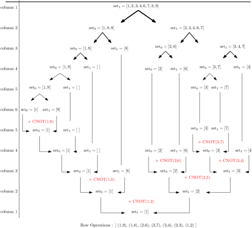
Figure 1: Illustration of the SelectAllRowOperations function on a specific example.

3.3 Bounding the CNOT Count

We denote with $C(n)$ the number of CNOTs required to synthesize a triangular operator $L$ of size $n$ with Algorithm 1. Given $1\leq k\leq n$, we consider $c(n,k)$ the number of row operations required to synthesize the first $k$ columns.

Once the first $k$ columns are synthesized the $n\times k$ block matrix $L[:,1:k]$ is equal to the matrix $\begin{pmatrix}I_{k}\\ 0\end{pmatrix}$ and we are left with the sub-matrix $L[k+1:end,k+1:end]$ to synthesize. Then we have

$$\forall k\geq 1,\;C(n)\leq c(n,k)+C(n-k)$$

and the total number of row operations to synthesize $L$ is upper bounded by

$$C(n)\qquad\leq\qquad\sum_{i=1}^{m}c\left(n-\sum_{j=1}^{i-1}k_{j},\,k_{i}\right)$$ (2)

where $k_{1},k_{2},...,k_{m}$ can represent any partition of $L$ into $m$ sub-blocks, i.e., $m$ positive integers such that $\sum_{i=1}^{m}k_{i}=n$. By considering the worst-case scenario for each block we do not take into consideration the side effects of the row operations that were applied on the first blocks and that could have an impact on the remaining matrix. Especially when looking strictly at one block, one can easily see that some row operations will only zero one element at a time in a block — the rightmost elements — but will certainly have an impact on the next block: by not considering this effect, we weaken our upper bound but the proof of the inequality (2) is straightforward.

We now turn to an estimation of an upper bound of $c(n,k)$. Considering a block of size $(n,k)$ and assuming that $k<\log_{2}(n)$, the algorithm process is the following :

• as there can be at most $2^{k}$ different bitstrings of $k$ bits, $n-2^{k}$ row operations at most will be used to zero the duplicate rows.

• We are left with a rectangular block of size $(2^{k},k)$. Using a similar argument we can zero $k-1$ bits of $2^{k-1}$ different rows by using one row operation for each, then the remaining bit on these rows can be zeroed with one row operation. We are now left with a block of size $(2^{k-1},k)$, we zero $k-2$ bits of $2^{k-2}$ rows with one row operation each and the two remaining bits on these rows can be zeroed with two row operations. Repeating this process until the whole block has been reduced to $\begin{pmatrix}I\\ 0\end{pmatrix}$, we perform at most

  $$2^{k-1}\times(1+1)+2^{k-2}\times(1+2)+2^{k-3}\times(1+3)...=2^{k+1}\times\sum_{j=2}^{k+1}j/2^{j}\leq 3\times 2^{k}$$

  row operations. We can save some row operations because the right upper triangular part of the block is already zeroed (as $L$ is triangular) but we neglect them for simplicity.

So we have the estimation

$$c(n,k)\leq n+2^{k+1}.$$ (3)

From this we can derive an upper bound for $C(n)$. We replace Eq. (3) in Eq. (2) :

$$C(n)\leq\sum_{i=1}^{m}\left(n-\sum_{j=1}^{i-1}k_{j}+2^{k_{i}+1}\right).$$

As $n-\sum_{j=1}^{i-1}k_{j}=\sum_{j=i}^{m}k_{j}$ for any $i$ we rewrite the upper bound

$$C(n)\leq\sum_{i=1}^{m}\left(2^{k_{i}+1}+\sum_{j=i}^{m}k_{j}\right)$$

$$C(n)\leq\sum_{i=1}^{m}\left(2^{k_{i}+1}+ik_{i}\right).$$ (4)

For simplicity we assume that $k_{1}=k_{2}=...=k_{m-1}=k$. We also assume that $k_{m}=n-\sum_{i=1}^{m-1}k_{i}=k$ and $m=n/k$ because it does not affect the results.

Replacing in Eq. (4):

$$C(n)\leq m2^{k+1}+k\frac{m(m+1)}{2}=\frac{n^{2}}{2k}+\frac{n}{k}2^{k+1}+\frac{n}{2}$$ (5)

We now prove two things:

1. we show that our upper bound is better than the one given in [38].

2. we prove that the asymptotic complexity is at most $n^{2}/\log_{2}(n)$.

1. Taking $k=\alpha\log_{2}(n)$ with $0<\alpha<1$, we have

$$2\times C(n)<\frac{n^{2}}{\alpha\log_{2}(n)}+\frac{4n^{1+\alpha}}{\alpha\log_{2}(n)}+n.$$ (6)

where the multiplication by $2$ gives an upper bound for the synthesis of a generic operator. This is a direct improvement over the upper bound in [38] given by

$$\text{total row op. \cite[cite]{[\@@bibref{}{patel2008optimal}{}{}]}}\leq\frac{n^{2}}{\alpha\log_{2}(n)}+2n^{1+\alpha}+\text{ negligible terms}$$ (7)

provided $\frac{4}{\alpha\log_{2}(n)}<2$ which is the case if $n$ is sufficiently large. For instance, with $\alpha=1/2$ then $n>16$ is sufficient.

2. The coefficient of the leading term in Eq (6) is $1/\alpha$, yet taking the limit $\alpha\to 1$ in Eq. (6) leads to a complexity of $5n^{2}/\log_{2}(n)$. Instead, taking $k=\log_{2}(n)-p$ for some $p$, we have

$$2\times C(n)<\frac{n^{2}}{\log_{2}(n)}\times\frac{1}{1-p/\log_{2}(n)}\times\left(1+\frac{4}{2^{p}}\right)+n.$$

By choosing carefully $p$, for instance $p=\sqrt{\log_{2}(n)}$, we get

$$2\times C(n)<a(n)\times\frac{n^{2}}{\log_{2}(n)}+n$$

with $a(n)=\frac{1}{1-1/\sqrt{\log_{2}(n)}}\times\left(1+\frac{4}{2^{\sqrt{\log_{2}(n)}}}\right)$. As $a(n)\to 1$ this proves that the asymptotic complexity is $n^{2}/\log_{2}(n)$.

We improve the upper bound Eq. (7) in two ways: we ensure that the coefficient of the leading term is $1$ and we avoid other terms that distort the real complexity. Especially if one wants to have the best asymptotic complexity with [38, Algo. 1] by choosing $\alpha$ arbitrarily close to 1, the term $n^{1+\alpha}$ becomes arbitrarily close to $n^{2}$ and its impact is not negligible until very large values of $n$. Even with intermediate values of $n$, for example $n=1000$, then $a(n)\approx 2.12$. To have the same leading term we have to choose $\alpha=1/2.12$. With these values we now have

$$\frac{2n^{1+\alpha}+n^{2}/(\alpha\log_{2}(n))}{n^{2}/(\alpha\log_{2}(n))}\approx 1.25$$

which means that the term $2n^{1+\alpha}$ increases the upper bound by 25%.

Discussion.

The main result we want to emphasize is that the upper bound in Eq. (4) is true for any partitioning of the matrix $L$. This means it performs better than any partitioning method unless a more efficient method for synthesizing one block is found. Notably, given $k_{1}=k_{2}=...=k_{m-1}=k$ the size of the block used for [38, Algo. 1] , it is clear that the row operations done in [38, Algo. 1] to zero an entire k-bit row will also be performed by our algorithm. Then we are left with a sub-matrix to synthesize for which [38, Algo. 1] will use a Gaussian Elimination method whereas our algorithm will perform recursively by first zeroing the bitstrings of size $k-1$. In the worst case our algorithm will only zero one element at a time like the Gaussian elimination algorithm.

This gives insights about the advantage of GreedyGE over [38, Algo. 1] . When [38, Algo. 1] performs a standard Gaussian elimination process to zero some elements, we somewhat perform [38, Algo. 1] on a smaller sub-matrix. Thus, at these steps of the algorithm, we expect to have the same gain in the number of row operations than [38, Algo. 1] has compared to the classical Gaussian elimination algorithm. Consequently, although we cannot theoretically claim that our algorithm always generates shorter circuits than [38, Algo. 1] — as we cannot claim that [38, Algo. 1] always performs better than standard Gaussian elimination — we have strong confidence that our algorithm provides better results most of the time — for the same reasons that [38, Algo. 1] gives most of the time better results than the Gaussian elimination algorithm. This assertion is empirically verified in our benchmarks, see Chapter 6.

4 Extending GreedyGE to General Operators

So far we have presented an algorithm for the synthesis of triangular operators. To extend this to generic linear reversible operators $A$ we give two strategies:

• we can modify our algorithm for triangular operators such that it transforms $A$ into an upper triangular operator $U$ on which we apply our unmodified algorithm,

• we can rely on an LU decomposition to factorize $A$ into the product of two triangular operators. Then the concatenation of the circuits implementing $U$ and $L$ yields a circuit implementing $A$.

4.1 Modification of FastGreedyGE

Algorithm 2 works even if the input operator is not lower triangular. In the outer for-loop, during the $j$-th iteration the algorithm will zero the sub-diagonal elements of the $j$-th column provided that the element $A[j,j]$ is equal to $1$. So all we need to do is adding an extra row operation to make sure that $A[j,j]=1$ is satisfied. If $A[j,j]=1$ then we do nothing otherwise we choose among the rows ${[\![}j+1,n{]\!]}$ whose $j$-th element is $1$ the one that zeroes the largest number of right elements of the j-th row so that when executing FastGreedyGE on the future $U$ operator we save some row operations. Overall this increases the CNOT count by at most $n$ so it is negligible in the derivation of the upper bound above.

4.2 Optimizing the Choice of $L$ and $U$

An LU decomposition provides a way to decompose an operator into two simpler sub-operators. Ideally, the path from the identity to the target operator given by the concatenation of the paths of two sub-operators would be close to the optimal path. In our case, it is very unlikely that an LU decomposition would give such an ideal decomposition because the structure of triangular operators is too specific. Nonetheless, the matrices L and U in the LU decomposition are not unique and we can optimize the factorization by choosing appropriate $L$ and $U$ operators such that we minimize the overall complexity of the final reversible circuit. In this section, we report several strategies to choose the matrices L and U.

If we allow row and column permutations, we can compute the LU decomposition of an operator $A$ following this algorithm:

1. Choose a row vector $v=A[i,:]$ and a column $j$ for which $A[i,j]=1$.

2. Set the first line of $U$ to $v$ and set the first column of $L$ to $A[:,j]$.

3. Update the matrix $A$, first by left-applying the gate $\text{SWAP}(i,1)$ and right-applying the gate $\text{SWAP}(j,1)$. Then add the vector $v$ to every row $A[k,:]$ where $A[k,1]=1$. Finally we are left with a matrix $A$ with zeroed first column and first row.

4. Repeat the algorithm on this updated $A$ until we obtain the null matrix.

At the end of the algorithm we have the relation

$$P_{1}AP_{2}=LU$$

where $P_{1},P_{2}$ are permutation matrices. $P_{1}$ is the concatenation of the SWAP gates that were left-applied to $A$ and $P_{2}$ is the concatenation of the SWAP gates that were right-applied to $A$. After the synthesis of $L$ and $U$ we can commute the gates with $P_{2}$ and have

$$A=P_{1}^{-1}P_{2}^{-1}L^{\prime}U^{\prime}$$

and we transfer the permutation matrix $P_{1}^{-1}P_{2}^{-1}$ to the end of the total circuit. $L^{\prime}$ and $U^{\prime}$ are triangular operators up to a permutation of their rows and columns.

At each step of the algorithm, we have several choices for the row and column vectors. We aim to construct $L$ and $U$ such that their synthesis will give short circuits. To do so we tried different strategies :

• First, if we believe that sparse $L$ and $U$ matrices can be implemented with shorter circuits, a first approach consists in choosing the row and column with smallest Hamming weights: this is the “sparse” approach.

• Secondly, we can adopt a "minimizing cost" approach. If the updated matrix $A^{\prime}$ minimizes a cost function then the synthesis of $A^{\prime}$ will require a shorter circuit. We choose the cost function to be the number of ones and we choose among all the possible rows and columns the pair that minimizes the number of ones in $A^{\prime}$.

These decompositions transform a general operator $A$ into two operators $L,U$ with specific structures. Triangular operators are easier to synthesize but this also limits the optimality of the solution. Because we force the algorithm to synthesize two matrices with a specific structure, it is very unlikely that we can perform an optimized synthesis by going through this forced path. This also gives insights into the question about the global optimality of our algorithm: even if we use an optimal algorithm for synthesizing a triangular operator it is very unlikely that we can get an optimal solution for the whole synthesis. Our algorithm gives asymptotic optimal results in the worst case but will be suboptimal for specific operators. Notably, if the operators can indeed be synthesized with a small circuit, direct greedy methods have shown encouraging results. In the next section, we will review the greedy method used in the literature and propose an extension of this framework to improve the scalability of this kind of algorithms.

5 Pathfinding Based Algorithms

The problem of linear reversible circuit synthesis can fit into a more generic problem called "pathfinding". In a pathfinding problem, we are generally given a starting state, a target state, and a set of operators that dictates the reachable states from a specific state. Then the goal is to find a path from the starting state to the goal state and the shorter the path is, the better it is. The reformulation of linear reversible circuit synthesis into a pathfinding problem is straightforward: the starting state is the operator $A$ we want to implement, the goal state is the identity operator and the available operators are all the elementary row and column operations.

This field of research in AI has been very active for the last decades and we can rely on many algorithms to solve our problem. The most famous one is probably the A* algorithm and all its derivatives (IDA* [22], Weighted A* [23], Anytime A* [26], etc.). These algorithms have been successfully used to solve toy problems (Rubik’s cube, Tile puzzles, Hanoi towers, Top Spin puzzle) but also concrete problems in video games [2], robotics [26, 2], genomics [46, 15, 44, 18], planning [7, 15], etc. Yet we are quickly faced with some crucial limitations :

• First the size of the search space grows much faster in our case than in any of the cases mentioned above. To give an order of magnitude, in [43] they compare greedy search algorithms - a subclass of pathfinding algorithms known for providing suboptimal solutions very quickly - and they highlight time and memory limitations of some algorithms especially on the largest problem they ran on: the 48-puzzle. The 48-puzzle and its variations (8-puzzle, 15-puzzle) are sliding puzzles. In the case of the 48-puzzle, 48 tiles are arranged in a $7\times 7$ square with one tile missing. The goal of the puzzle is to order the tiles by moving the empty space around. For this specific problem the authors of [43] show that the computational time for most of the pathfinding algorithms they consider increases substantially while providing solutions of poor quality. The number of different positions in the 48-puzzle is equal to $49!/2\approx 3\times 10^{62}$. This is less than the number of linear reversible functions on $15$ qubits. As we expect to be able to synthesize circuits on $50$ qubits and even more, it is clear that we cannot use all the pathfinding algorithms in the literature.

• Secondly we need a function that will evaluate the distance between the current state and the target state. The properties of this function, usually called the heuristic, will deeply influence the performance of the pathfinding algorithms. Its goal is to guide the search by giving priority to more promising states and prune a whole part of the search space. More generally there are two sources of improvement for a pathfinding algorithm: the accuracy of the heuristic function and the management of the path discovery, i.e., what strategy do you employ to explore the search space. If the latter can be quite independent of the problem, the former is very problem-specific and unfortunately to our knowledge no good heuristics exist that satisfy good theoretical properties. For instance, for A* to provide an optimal solution we need the heuristic to be admissible and consistent, i.e., it must always underestimate the length of the optimal path and the value of the heuristic should always decrease of at most one after the application of one elementary operation. By taking a function that always returns 0 we have an admissible and consistent heuristic but the search will result in a brute-force search. Generally to obtain an admissible heuristic we can consider a simpler version of our problem and the optimal solution of this problem gives an underestimation of the distance to the target state. In the case of linear reversible circuits, the closest simplified subproblem we found is the Shortest Linear Straight-Line Program [8] but this problem is also NP-hard and cannot be approximated exactly by a polynomial algorithm.

For all these reasons, we believe that using the standard A* algorithm or its derivatives is a dead end. Instead of that, we focused our work on greedy best-first search algorithms that can be seen as a cost minimization/discrete gradient descent approach. It has been shown that the heuristics that are efficient for this kind of search are different than the ones for A* algorithms [42], so we expect that we can exploit the properties of the matrix $A$ of our operator to guide our search.

To our knowledge, the cost minimization approach for linear reversible circuits synthesis has only been investigated in [40]. Yet, with their methods, the authors can only synthesize circuits on at most $25$ qubits. More crucially, they did not investigate the behavior of their methods when the resulting circuits are supposed to be small. According to us, this is a behavior that has to be considered because as we will see the results of the methods drastically change depending on the size of the optimal circuits.

We consider two different heuristic functions to guide our search. The first one, already used in [40], is the function

$$h_{\text{s}um}(A)=\sum_{i,j}a_{i,j}$$

that is to say the number of ones in the matrix $A$. We also propose a new cost function to solve this problem, it is defined by

$$h_{\text{p}rod}(A)=\sum_{i=1}^{n}\log\left(\sum_{j=1}^{n}a_{i,j}\right)$$

which corresponds to the log of the product of the number of ones on each row. These two cost functions reach their minimum when $A$ is a permutation matrix, motivating their use in a cost minimization process. If the cost function $h_{\text{s}um}$ seems the first natural choice, we propose the cost function $h_{\text{p}rod}$ because it gives priority to "almost done" rows. Namely, if one row has only a few nonzero entries, the minimization process with $h_{\text{p}rod}$ will treat this row in priority and then it will not modify it anymore. This enables to avoid a problem which one meets with the cost function $h_{\text{s}um}$ where one ends up with a very sparse matrix but where the rows and columns have few nonzero common entries. This type of matrix represents a local minimum from which it can be difficult to escape. With this new cost function, as we put an additional priority on the rows with few remaining nonzero entries, we avoid this pitfall.

An important improvement given in [40] is to add the value of the cost function applied to the inverse as well, i.e.,

$$H_{\text{s}um}(A)=h_{\text{s}um}(A)+h_{\text{s}um}(A^{-1}),$$

$$H_{\text{p}rod}(A)=h_{\text{p}rod}(A)+h_{\text{p}rod}(A^{-1}).$$

Again, these two new cost functions are minimum when $A$ is a permutation. As we will see adding the cost value of the inverse tightens the possible paths and can improve the results because we escape more easily from local minima during the search.

We now give a few details on our implementation. We directly work on a cost matrix that stores the impact of each possible CNOT on the cost function. Namely let $M$ be such matrix, then $M[i,j]=h(E_{ij}A)-h(A)$ where $h\in\{h_{\text{s}um},h_{\text{p}rod}\}$. We can define similar cost matrices for $A^{-1}$ and for column operations. Overall we have four matrices $M_{A,\text{row}},M_{A,\text{col}},M_{A^{-1},\text{row}},M_{A^{-1},\text{col}}$. Note that $(E_{ij}A)^{-1}=A^{-1}E_{ij}$ so a row operation $\text{Row}(i,j)$ on $A$ is a column operation $\text{Col}(j,i)$ on $A^{-1}$. The cost minimization algorithm is simple if we work with such matrices: at each iteration we look for the pair $(i,j)$ that minimizes $\min(M_{A,\text{row}}[i,j]+M_{A^{-1},\text{col}}[j,i],M_{A,\text{col}}[i,j]+M_{A^{-1},\text{row}}[j,i])$, we update $A$ and $A^{-1}$ and we pursue the algorithm until $A$ is a permutation matrix. The advantage of working on cost matrices rather than directly on $A$ is that the update of the $M$’s is cheaper than updating $A$ and computing the costs. For instance, suppose we apply $\text{Row}(i,j)$ to $A$, then if $h=h_{\text{sum}}$ the impact on the cost function of any row operation that does not involve row $j$ will be the same than before the application of $\text{Row}(i,j)$. This means that we only need to update $M_{A,\text{Row}}[i,j],M_{A,\text{Row}}[j,i],M_{A^{-1},\text{Col}}[i,j],M_{A^{-1},\text{Col}}[j,i]$ for $i=1..n$. The updates of $M_{A,\text{Col}}$ and $M_{A^{-1},\text{Row}}$ are also simpler because only one element of each column of $A$ has been modified. However, for our new cost function the updates are not that simple and it will have an impact on the computational time.

With cost minimization techniques it is not rare to fall into local minima. In that case we simply select among the best operations a random one and pursue the search. If the number of iterations exceeds a certain number then we consider that the algorithm is stuck in a local minimum and we stop it.

6 Benchmarks

This section presents our experimental results. We have the following algorithms to benchmark:

• GreedyGE from Sections 3 and 4,

• cost minimization techniques from Section 5,

The state-of-the-art algorithms are the following:

• The PMH algorithm [38, Algo. 1] ,

• The algorithm based on the syndrome decoding problem from [9].

Two kinds of datasets are used to benchmark our algorithms:

• First, a set of random operators. The test on random operators gives an overview of the average performance of our algorithm. We generate random operators by creating random CNOT circuits. Our routine takes two inputs: the number of qubit $n$ and the number of CNOT gates $k$ in the random circuit. Each CNOT is randomly placed by selecting a random control and a random target and the simulation of the circuit gives a random operator. Empirically we noticed that when $k$ is sufficiently large — $k=n^{2}$ is enough — then the operators generated have strong probability to represent the worst case scenarii.

• Secondly, a set of reversible functions, given as circuits, taken from Matthew Amy’s github repository [3]. This experiment shows how our algorithms can optimize useful quantum algorithms in the literature like the Galois Field multipliers, integer addition, Hamming coding functions, the hidden weighted bit functions, etc.

To evaluate the performance of our algorithms for the random set, two types of experiments are conducted:

1. a worst-case asymptotic experiment, namely for increasing problem sizes $n$ we generate circuits with $n^{2}$ gates and we compute the average number of gates for each problem size. This experiment reveals the asymptotic behavior of the algorithms and gives insights about strict upper bounds on their performance.

2. a close-to-optimal experiment, namely for one specific problem size we generate operators with different number of gates to show how close to optimal our algorithms are if the optimal circuits are expected to be smaller than the worst case.

All our algorithms are implemented in Julia [6] and executed on the ATOS QLM (Quantum Learning Machine) whose processor is an Intel Xeon(R) E7-8890 v4 at 2.4 GHz.

6.1 Random Operators

6.1.1 GreedyGE

First, we present the worst-case asymptotic experiment with the following algorithms:

• GreedyGE with standard LU decomposition,

• Syndrome decoding with the cost minimization heuristic with unlimited width and depth 1,

• Syndrome decoding with the integer programming solver (Coin-or branch and cut solver),

• Syndrome decoding with the cost minimization heuristic (width=Inf, depth=1) and $50$ random changes of basis, the “Information Set Decoding” (ISD) case.

• Syndrome decoding with the cost minimization heuristic with width 60 and depth 2,

• Syndrome decoding with the cost minimization heuristic with width 15 and depth 3,

The results are given in Fig 2. For the sake of clarity, instead of showing the circuit size we plot the ratio between the circuit size given by our method and the circuit size given by the PMH algorithm. So if the ratio is below $1$ this means that we outperform the state-of-the art method [38, Algo. 1] . We also have a better view of which algorithm is better in which qubit range. We stopped the calculations when the running time was too large for producing benchmarks within several hours.

Overall, for the considered range of qubits, GreedyGE outperforms [38, Algo. 1] . As the number of qubits increases the syndrome decoding based algorithm performs worse and GreedyGE eventually produces the shortest circuits when $n>120$. Notably, the average gain over the PMH algorithm stabilizes around 25%. On the other hand the syndrome decoding based algorithms performances deteriorate as $n$ increases or the algorithm cannot terminate when the heuristic is too costly. Therefore, for large $n$, GreedyGE is the best method so far. GreedyGE is also fast: we compare the computational time of GreedyGE against the standard Gaussian elimination and the PMH algorithm. The results are given in Table 1. Not only GreedyGE produces the smallest circuits but in addition it is the fastest method to our knowledge.

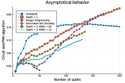
Figure 2: Average performance of GreedyGE and the Syndrome Decoding based algorithms versus the PMH algorithm.

Table 1: Computational time of GreedyGE vs PMH and standard Gaussian elimination algorithms.

Algorithm	Average computational time (s)
	$n=10$	$n=100$	$n=500$	$n=1000$	$n=5000$
Gaussian elimination	0.00004	0.00125	0.14	1.2	140
PMH algorithm	0.00015	0.006	0.75	7	980
GreedyGE	0.00015	0.0035	0.1	0.6	45

Next, we show the impact of the choice of the LU decomposition. We provide results with GreedyGE considering it can be directly transposed to the syndrome decoding based algorithms as well. We perform the close-to-optimal experiment with the GreedyGE and three different LU decompositions:

• a standard LU decomposition for matrix in $\mathbb{F}_{2}$, taken from the Julia package Nemo [10],

• the LU decomposition algorithm with the "sparse" strategy,

• the LU decomposition algorithm with the "cost minimization" strategy.

The experiment is done on $60$ qubits. We also add the best method for this problem size: the syndrome decoding based algorithm with the "Information Set Decoding" strategy. The results are given in Fig 3. Computing more efficient LU decompositions has almost no effect on the worst-case results but provides some improvements when the input circuits are smaller. There is no significant difference between the two strategies "sparse" and "cost minimization" in terms of circuit sizes but the running time is much lower for the sparse approach so we would privilege it. This improvement also benefits the syndrome decoding based method as it also relies on an LU decomposition. On the other hand we also see that there is no obvious advantage of using GreedyGE instead of the syndrome decoding based methods when the optimal circuit is expected to be small.

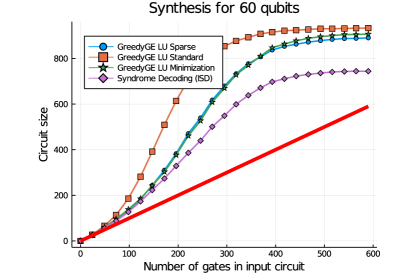
Figure 3: Performance of GreedyGE with different LU decompositions vs Syndrome Decoding on 60 qubits for different input circuit sizes.

6.1.2 Path Finding Methods

We now evaluate the performance of purely greedy methods. We remind that we have four cost functions to study:

• $h_{\text{s}um}(A)=\sum_{i,j}a_{i,j}$,

• $h_{\text{p}rod}(A)=\sum_{i=1}^{n}\log\left(\sum_{j=1}^{n}a_{i,j}\right)$,

• $H_{\text{s}um}(A)=h_{\text{s}um}(A)+h_{\text{s}um}(A^{-1})$,

• $H_{\text{p}rod}(A)=h_{\text{p}rod}(A)+h_{\text{p}rod}(A^{-1})$.

First, we show the asymptotic behavior of those four methods. The results are given in Fig 4. The first graph in Fig 4(a) shows that the cost function $h_{\text{s}um}$ does not scale well with the number of qubits so we decide to remove it for clarity. The new graph is given in Fig 4(b). We notice two things: first, the cost function $H_{\text{p}rod}$ always underperforms $h_{\text{p}rod}$, secondly both $H_{\text{s}um}$ and $h_{\text{p}rod}$ outperform our syndrome decoding based algorithm for small problem sizes ($n<30$) but with an advantage for $H_{\text{s}um}$ when $n<25$. There is a thin window — between $25$ and $30$ qubits — where it is preferable to use $h_{\text{p}rod}$ instead of $H_{\text{s}um}$.

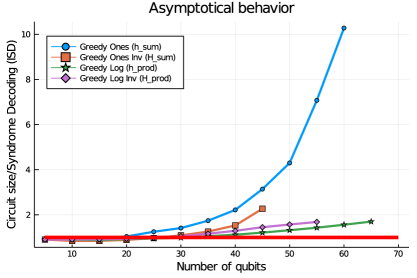
(a) Average performance of {$h_{\text{s}um},h_{\text{p}rod},H_{\text{s}um},H_{\text{p}rod}$} vs Syndrome decoding (Information Set Decoding).

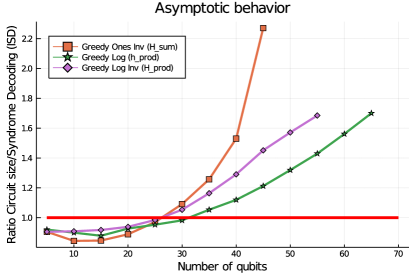
(b) Same graph as in Fig 4(a) without $h_{\text{s}um}$.

Figure 4: Average performance of Cost minimization techniques vs Syndrome decoding (Information Set Decoding).

The results given in Fig 4 are mainly there to discredit two of the four cost functions: $h_{\text{s}um}$ and $H_{\text{p}rod}$. The result that really interests us is that of the close-to-optimal experiment, here on $50$ qubits and given in Fig 5. For this problem size on the worst case the syndrome decoding based algorithm outperforms our greedy methods. But when we are not in the worst case the results are completely different: the greedy methods follow more faithfully the bound $y=x$ than the syndrome decoding based algorithm. We have to wait input circuits of size $300$ for the syndrome decoding algorithm to be better. The greedy algorithm based on the cost function $h_{\text{p}rod}$ produces much more stable results than the one with the cost function $H_{\text{s}um}$. For the cost function $H_{\text{s}um}$ the variance is extremely large because the method struggles finding a global minimum. However, it is $H_{\text{s}um}$ that produces the best results most of the time in the range of size $0-300$. Again there is a thin window where it may be relevant to use $h_{\text{p}rod}$ instead of $H_{\text{s}um}$.

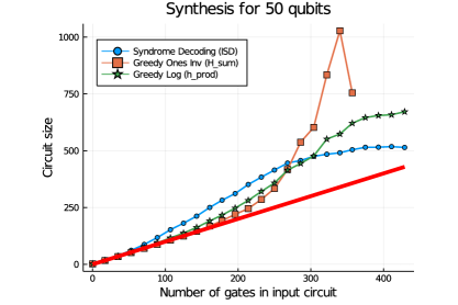
Figure 5: Performance of Cost minimization techniques vs Syndrome Decoding on 50 qubits for different input circuit sizes.

6.1.3 Conclusion: Combining the Methods

Each method has its own range of validity:

• GreedyGE is suited when the number of qubits exceeds $120$, it outperforms the PMH algorithm and our other algorithms in both circuit size and computational time.

• The syndrome decoding based algorithms must be used for intermediate problem sizes ($30<n<120$) with the best possible solver of the syndrome decoding problem (in order: integer programming, Information Set Decoding if $n<70$, maximum depth otherwise). Both GreedyGE and the family of syndrome decoding based algorithms are state of the art in a worst case scenario.

• When the output circuit is expected to be small, or when $n<30$, then direct greedy methods have shown to produce the best results. The proposal of a new cost function paid off as this offers a more scalable direct greedy search. However, the moment when our new custom function outperforms the one proposed in [40] coincides with the moment when the syndrome decoding based algorithm also outperforms the direct greedy search. More investigation needs to be done to clarify which cost function should be preferred and when.

Given the variety of methods, each providing the best results in particular cases, the best method when trying to synthesize an operator would be simply to test each method and to keep the best result. Except for the direct greedy methods, the computational time of each method is well understood. Given a specific problem size, it is easy to know which method can be used and how long it will take. It is more delicate with the direct greedy methods, we have to set a limit in the maximum number of iterations before considering that the search will not converge to a solution.

6.2 Benchmarks on Reversible Functions

We apply our CNOT circuit synthesis to the optimization of quantum algorithms. A library to evaluate the quality of a quantum compiler is a library of reversible functions consisting of adders, Hamming coding functions, multipliers, etc. This library is a standard benchmark for circuit optimization algorithms and is used in recent articles about quantum circuit optimization [17, 5, 4, 35]. However, we must be aware that our results can only be compared to those using the same methodology. There are many other methods for the synthesis and optimization of reversible circuits [39], notably for the synthesis of oracles [30, 32], which we do not take into account here. The aim of this section is to show that our methods can bring promising results on specific circuits and that it will be interesting to apply it on other classes of circuits, but it will also be necessary to put it in perspective with other methods.

The original circuits are from Matthew Amy’s github Feynman repository [3].

Recent quantum compilers mainly focused on the T-count or T-depth optimization of quantum circuits but these optimizations often lead to an increased CNOT count [17, 5]. Although it is experimentally more costly to implement a T gate, the total number of CNOT gates in a quantum circuits should not be too large otherwise the CNOT cost of the total circuit will not be negligible. In practice it may even be possible that the CNOT cost represents the most costly part of a quantum circuit [28] and it cannot be neglected.

In [4] the algorithm Gray-Synth for the optimization of the CNOT count in CNOT+T circuits is proposed. It efficiently reduces the total number of CNOT gates but it comes at the price of an increased T-depth. Here we show that, using our methods for CNOT circuit synthesis, one can reduce significantly the CNOT count without paying the price of increasing the T depth. We used the C++ implementation of Matthew Amy’s Tpar algorithm to produce optimized circuits with low T-count and T-depth. We post process the circuits by re-synthesizing any chunk of purely CNOT circuits. It is possible to further optimize the synthesis of the CNOT+T circuits, using for instance the TODD optimizer [17] but as we are concerned about showing the impact of our method on the CNOT count and the T-depth we did not pursue the optimization to have a lower T-count so that we can directly compare against the results from [4].

The results are given in Table 2. For each reversible function we provide the results (T-count, T-depth, Total depth) of different methods implementing it. Namely, the original circuits, the circuits optimized solely with the Tpar algorithm and GraySynth as the state-of-the-art methods and the circuits optimized with the Tpar method and our own method, i.e., a mix of GreedyGE, the syndrome decoding based methods and the purely greedy methods. For each CNOT circuit we keep the best result encountered. To generate the Gray-Synth results we used the Haskell implementation, still from [3]. The savings given always compare against the circuits given by solely the Tpar algorithm. We notice several interesting points:

• we cannot decrease the CNOT count as much as with GraySynth, but we still manage to decrease the CNOT count consistently and above all we do not modify the T-depth. Our circuits therefore represent a tradeoff between the T-cost the CNOT-cost.

• We also considerably reduce the total depth of the circuits, making their execution faster on NISQ architectures. This is explained by the fact that most of the CNOT circuits involved in those reversible functions are elementary operators, requiring only a few CNOTs to be implemented. Therefore the size and the depth are very close and greedy methods find close-to-optimal implementations.

To illustrate our last statement, we kept track of the best algorithm that was used to compute each CNOT sub-circuit that appeared in the synthesis of one reversible function. The results are given in Table 3. Most of the time, both purely greedy methods and the syndrome decoding based methods provide the best results. According to us, this highlights the simplicity of the operators to synthesize otherwise there would be many more cases where we would observe a difference of even one CNOT. Overall, for this library of reversible functions, the use of methods other than the pure greedy methods is useless. This is not surprising as the number of qubits never exceeds $40$ except for three operators. For such small problem sizes, we saw that pure greedy methods always outperform the other methods, in addition to the fact that we have strong suspicions that the majority of the operators encountered are easy to synthesize. We note the interest of using the cost function $h_{\text{prod}}$ as an alternative because in some cases it allows to synthesize operators more efficiently.

Table 2: CNOT optimization of a library of reversible functions with several CNOT circuits synthesis methods.

Function	#$n$	Original				Tpar				Tpar + GraySynth				Tpar + CNOT size opt.
		T-count	T-depth	CNOT count	Depth	T-count	T-depth	CNOT count	Depth	T-count	T-depth	CNOT count	Depth	T-count	T-depth	CNOT count	Depth
Adder_8	$24$	$399$	$69$	$466$	$223$	$213$	$30$	$741$	$302$	$215$	$74$ ( $147\%$)	$399$ ($-46\%$)	$257$ ( $-15\%$)	$213$	$30$	$491$ ( $-34\%$)	$204$ ( -32%)
barenco_tof_10	$19$	$224$	$96$	$224$	$288$	$100$	$43$	$332$	$272$	$100$	$81$ ( $88\%$)	$146$ ($-56\%$)	$264$ ( $-3\%$)	$100$	$43$	$188$ ( $-43\%$)	$217$ ( -20%)
barenco_tof_3	$5$	$28$	$12$	$28$	$36$	$16$	$8$	$52$	$60$	$16$	$16$ ( $100\%$)	$20$ ($-62\%$)	$40$ ( $-33\%$)	$16$	$8$	$26$ ( $-50\%$)	$34$ ( -43%)
barenco_tof_4	$7$	$56$	$24$	$56$	$72$	$28$	$13$	$96$	$96$	$28$	$26$ ( $100\%$)	$38$ ($-60\%$)	$64$ ( $-33\%$)	$28$	$13$	$50$ ( $-48\%$)	$61$ ( -36%)
barenco_tof_5	$9$	$84$	$36$	$84$	$108$	$40$	$18$	$134$	$123$	$40$	$34$ ( $89\%$)	$56$ ($-58\%$)	$88$ ( $-28\%$)	$40$	$18$	$73$ ( $-46\%$)	$89$ ( -28%)
csla_mux_3	$15$	$70$	$21$	$90$	$67$	$62$	$8$	$379$	$210$	$62$	$28$ ( $250\%$)	$115$ ($-70\%$)	$91$ ( $-57\%$)	$62$	$8$	$187$ ( $-51\%$)	$81$ ( -61%)
csum_mux_9	$30$	$196$	$18$	$196$	$59$	$84$	$6$	$366$	$153$	$84$	$16$ ( $167\%$)	$160$ ($-56\%$)	$78$ ( $-49\%$)	$84$	$6$	$179$ ( $-51\%$)	$70$ ( -54%)
cycle_17_3	$35$	$4739$	$2001$	$4742$	$5974$	$1944$	$562$	$6608$	$5231$	$1955$	$1857$ ( $230\%$)	$3040$ ($-54\%$)	$5698$ ( $9\%$)	$1944$	$562$	$4267$ ( $-35\%$)	$4229$ ( -19%)
GF($2^{10}$)_mult	$30$	$700$	$108$	$709$	$290$	$410$	$16$	$2206$	$1026$	$410$	$109$ ( $581\%$)	$648$ ($-71\%$)	$324$ ( $-68\%$)	$410$	$16$	$955$ ( $-57\%$)	$307$ ( -70%)
GF($2^{16}$)_mult	$48$	$1792$	$180$	$1837$	$489$	$1040$	$24$	$6724$	$2551$	$1040$	$585$ ( $2338\%$)	$1691$ ($-75\%$)	$1488$ ( $-42\%$)	$1040$	$24$	$2542$ ( $-62\%$)	$678$ ( -73%)
GF($2^{32}$)_mult	$96$	$7168$	$372$	$7292$	$1001$	$4128$	$47$	$34244$	$11520$	$4128$	$2190$ ( $4560\%$)	$6636$ ($-81\%$)	$5391$ ( $-53\%$)	$4128$	$47$	$10953$ ( $-68\%$)	$2113$ ( -82%)
GF($2^{4}$)_mult	$12$	$112$	$36$	$115$	$99$	$68$	$6$	$307$	$173$	$68$	$39$ ( $550\%$)	$106$ ($-65\%$)	$117$ ( $-32\%$)	$68$	$6$	$135$ ( $-56\%$)	$80$ ( -54%)
GF($2^{5}$)_mult	$15$	$175$	$48$	$179$	$130$	$115$	$9$	$502$	$259$	$115$	$51$ ( $467\%$)	$166$ ($-67\%$)	$152$ ( $-41\%$)	$115$	$9$	$209$ ( $-58\%$)	$107$ ( -59%)
GF($2^{6}$)_mult	$18$	$252$	$60$	$257$	$163$	$150$	$9$	$660$	$350$	$150$	$63$ ( $600\%$)	$235$ ($-64\%$)	$189$ ( $-46\%$)	$150$	$9$	$310$ ( $-53\%$)	$137$ ( -61%)
GF($2^{7}$)_mult	$21$	$343$	$72$	$349$	$195$	$217$	$12$	$996$	$490$	$217$	$75$ ( $525\%$)	$319$ ($-68\%$)	$224$ ( $-54\%$)	$217$	$12$	$442$ ( $-56\%$)	$184$ ( -62%)
GF($2^{8}$)_mult	$24$	$448$	$84$	$469$	$233$	$264$	$13$	$1254$	$619$	$264$	$87$ ( $569\%$)	$428$ ($-66\%$)	$266$ ( $-57\%$)	$264$	$13$	$588$ ( $-53\%$)	$224$ ( -64%)
GF($2^{9}$)_mult	$27$	$567$	$96$	$575$	$258$	$351$	$15$	$1712$	$810$	$351$	$95$ ( $533\%$)	$526$ ($-69\%$)	$283$ ( $-65\%$)	$351$	$15$	$753$ ( $-56\%$)	$266$ ( -67%)
grover_5	$9$	$336$	$144$	$336$	$457$	$154$	$51$	$499$	$477$	$154$	$130$ ( $155\%$)	$232$ ($-54\%$)	$440$ ( $-8\%$)	$154$	$51$	$331$ ( $-34\%$)	$384$ ( -19%)
ham15-high	$20$	$2457$	$996$	$2500$	$3026$	$1019$	$380$	$3427$	$2956$	$1019$	$839$ ( $121\%$)	$1588$ ($-54\%$)	$2583$ ( $-13\%$)	$1019$	$380$	$2183$ ( $-36\%$)	$2226$ ( -25%)
ham15-low	$17$	$161$	$69$	$259$	$263$	$97$	$33$	$471$	$360$	$97$	$83$ ( $152\%$)	$221$ ($-53\%$)	$271$ ( $-25\%$)	$97$	$33$	$280$ ( $-41\%$)	$223$ ( -38%)
ham15-med	$17$	$574$	$240$	$616$	$750$	$230$	$84$	$759$	$682$	$230$	$194$ ( $131\%$)	$368$ ($-52\%$)	$622$ ( $-9\%$)	$230$	$84$	$481$ ( $-37\%$)	$506$ ( -26%)
hwb6	$7$	$105$	$45$	$131$	$152$	$75$	$24$	$270$	$248$	$75$	$63$ ( $162\%$)	$111$ ($-59\%$)	$188$ ( $-24\%$)	$75$	$24$	$172$ ( $-36\%$)	$164$ ( -34%)
hwb8	$12$	$5887$	$2139$	$7970$	$7956$	$3531$	$860$	$22670$	$15838$	$3531$	$2752$ ( $220\%$)	$6841$ ($-70\%$)	$9338$ ( $-41\%$)	$3531$	$860$	$13353$ ( $-41\%$)	$9261$ ( -42%)
mod5_4	$5$	$28$	$12$	$32$	$41$	$16$	$6$	$48$	$57$	$16$	$15$ ( $150\%$)	$28$ ($-42\%$)	$51$ ( $-11\%$)	$16$	$6$	$32$ ( $-33\%$)	$39$ ( -32%)
mod_adder_1024	$28$	$1995$	$831$	$2005$	$2503$	$1011$	$258$	$3650$	$2560$	$1011$	$864$ ( $235\%$)	$1390$ ($-62\%$)	$2474$ ( $-3\%$)	$1011$	$258$	$2369$ ( $-35\%$)	$1913$ ( -25%)
mod_adder_1048576	$58$	$17290$	$7292$	$17310$	$21807$	$7298$	$1927$	$29794$	$19975$	$7323$	$6577$ ( $241\%$)	$11080$ ($-63\%$)	$20089$ ( $1\%$)	$7298$	$1927$	$19122$ ( $-36\%$)	$15286$ ( -23%)
mod_mult_55	$9$	$49$	$15$	$55$	$50$	$35$	$7$	$106$	$75$	$35$	$20$ ( $186\%$)	$40$ ($-62\%$)	$52$ ( $-31\%$)	$35$	$7$	$73$ ( $-31\%$)	$61$ ( -19%)
mod_red_21	$11$	$119$	$48$	$122$	$158$	$73$	$25$	$223$	$207$	$73$	$59$ ( $136\%$)	$102$ ($-54\%$)	$179$ ( $-14\%$)	$73$	$25$	$136$ ( $-39\%$)	$144$ ( -30%)
qcla_adder_10	$36$	$238$	$24$	$267$	$73$	$162$	$13$	$648$	$195$	$162$	$33$ ( $154\%$)	$225$ ($-65\%$)	$94$ ( $-52\%$)	$162$	$13$	$362$ ( $-44\%$)	$86$ ( -56%)
qcla_com_7	$24$	$203$	$27$	$215$	$81$	$94$	$12$	$371$	$154$	$94$	$31$ ( $158\%$)	$150$ ($-60\%$)	$89$ ( $-42\%$)	$94$	$12$	$202$ ( $-46\%$)	$76$ ( -51%)
qcla_mod_7	$26$	$413$	$66$	$441$	$197$	$231$	$28$	$813$	$296$	$237$	$67$ ( $139\%$)	$386$ ($-53\%$)	$212$ ( $-28\%$)	$231$	$28$	$479$ ( $-41\%$)	$188$ ( -36%)
qft_4	$5$	$69$	$48$	$48$	$142$	$67$	$44$	$96$	$185$	$67$	$60$ ( $36\%$)	$48$ ($-50\%$)	$163$ ( $-12\%$)	$67$	$44$	$56$ ( $-42\%$)	$150$ ( -19%)
rc_adder_6	$14$	$77$	$33$	$104$	$104$	$47$	$22$	$165$	$157$	$47$	$39$ ( $77\%$)	$79$ ($-52\%$)	$111$ ( $-29\%$)	$47$	$22$	$100$ ( $-39\%$)	$103$ ( -34%)
tof_10	$19$	$119$	$51$	$119$	$153$	$71$	$27$	$236$	$190$	$71$	$61$ ( $126\%$)	$86$ ($-64\%$)	$172$ ( $-9\%$)	$71$	$27$	$130$ ( $-45\%$)	$143$ ( -25%)
tof_3	$5$	$21$	$9$	$21$	$27$	$15$	$6$	$35$	$46$	$15$	$12$ ( $100\%$)	$16$ ($-54\%$)	$32$ ( $-30\%$)	$15$	$6$	$21$ ( $-40\%$)	$31$ ( -33%)
tof_4	$7$	$35$	$15$	$35$	$45$	$23$	$9$	$63$	$71$	$23$	$18$ ( $100\%$)	$26$ ($-59\%$)	$51$ ( $-28\%$)	$23$	$9$	$37$ ( $-41\%$)	$49$ ( -31%)
tof_5	$9$	$49$	$21$	$49$	$63$	$31$	$12$	$97$	$104$	$31$	$24$ ( $100\%$)	$36$ ($-63\%$)	$70$ ( $-33\%$)	$31$	$12$	$50$ ( $-48\%$)	$67$ ( -36%)
vbe_adder_3	$10$	$70$	$24$	$80$	$79$	$24$	$9$	$120$	$88$	$24$	$18$ ( $100\%$)	$54$ ($-55\%$)	$71$ ( $-19\%$)	$24$	$8$	$61$ ( $-49\%$)	$45$ ( -49%)
Mean savings (compared to Tpar)											+391.39%	-60.21%	-29.66%			-45.03%	-41.26%
Maximum savings (compared to Tpar)											+36%	-81%	-68%			-68%	-82%
Minimum savings (compared to Tpar)											+4560%	-42%	+9%			-31%	-19%

Table 3: Frequency of best performance of each algorithm during the optimization of reversible circuits. For each algorithm, the first column gives the number of times it has returned the best result (possibly other algorithms returned circuits of same size). The second column reports the number of times it was the only one to provide the best possible circuit.

Function	#$n$	#CNOT sub-circuits	PMH		GreedyGE		Syndrome (Information Set Decoding)		Syndrome (Depth 3)		Syndrome (IP)		Greedy Ones ($H_{\text{sum}}$)		Greedy Log ($h_{\text{log}}$)
			Best choice	Only Choice	Best choice	Only Choice	Best choice	Only Choice	Best choice	Only Choice	Best choice	Only Choice	Best choice	Only Choice	Best choice	Only Choice
Adder_8	$24$	60	12 (20%)	0 (0)	13 (22%)	0 (0%)	42 (70%)	0 (0%)	42 (70%)	0 (0%)	42 (70%)	0 (0%)	60 (100%)	2 (3%)	58 (97%)	0 (0%)
barenco_tof_10	$19$	99	29 (29%)	0 (0)	33 (33%)	0 (0%)	83 (84%)	0 (0%)	83 (84%)	0 (0%)	83 (84%)	0 (0%)	99 (100%)	0 (0%)	99 (100%)	0 (0%)
barenco_tof_3	$5$	14	8 (57%)	0 (0)	8 (57%)	0 (0%)	12 (86%)	0 (0%)	12 (86%)	0 (0%)	12 (86%)	0 (0%)	13 (93%)	0 (0%)	13 (93%)	0 (0%)
barenco_tof_4	$7$	27	12 (44%)	0 (0)	12 (44%)	0 (0%)	24 (89%)	0 (0%)	24 (89%)	0 (0%)	24 (89%)	0 (0%)	26 (96%)	0 (0%)	26 (96%)	0 (0%)
barenco_tof_5	$9$	39	16 (41%)	0 (0)	16 (41%)	0 (0%)	32 (82%)	0 (0%)	32 (82%)	0 (0%)	32 (82%)	0 (0%)	38 (97%)	0 (0%)	38 (97%)	0 (0%)
csla_mux_3	$15$	15	0 (0%)	0 (0)	0 (0%)	0 (0%)	8 (53%)	0 (0%)	8 (53%)	0 (0%)	8 (53%)	0 (0%)	15 (100%)	2 (13%)	10 (67%)	0 (0%)
csum_mux_9	$30$	14	1 (7%)	0 (0)	1 (7%)	0 (0%)	6 (43%)	0 (0%)	6 (43%)	0 (0%)	6 (43%)	0 (0%)	13 (93%)	4 (29%)	9 (64%)	0 (0%)
cycle_17_3	$35$	1436	219 (15%)	0 (0)	330 (23%)	0 (0%)	1094 (76%)	0 (0%)	1094 (76%)	0 (0%)	1094 (76%)	0 (0%)	1429 (100%)	23 (2%)	1412 (98%)	6 (0%)
GF($2^{10}$)_mult	$30$	20	0 (0%)	0 (0)	0 (0%)	0 (0%)	1 (5%)	0 (0%)	1 (5%)	0 (0%)	1 (5%)	0 (0%)	16 (80%)	13 (65%)	6 (30%)	3 (15%)
GF($2^{16}$)_mult	$48$	28	0 (0%)	0 (0)	0 (0%)	0 (0%)	2 (7%)	0 (0%)	2 (7%)	0 (0%)	2 (7%)	0 (0%)	18 (64%)	15 (54%)	11 (39%)	8 (29%)
GF($2^{32}$)_mult	$96$	51	0 (0%)	0 (0)	0 (0%)	0 (0%)	2 (4%)	0 (0%)	2 (4%)	0 (0%)	2 (4%)	0 (0%)	30 (59%)	28 (55%)	21 (41%)	19 (37%)
GF($2^{4}$)_mult	$12$	10	0 (0%)	0 (0)	0 (0%)	0 (0%)	3 (30%)	0 (0%)	3 (30%)	0 (0%)	3 (30%)	0 (0%)	9 (90%)	3 (30%)	6 (60%)	0 (0%)
GF($2^{5}$)_mult	$15$	13	1 (8%)	0 (0)	0 (0%)	0 (0%)	3 (23%)	0 (0%)	3 (23%)	0 (0%)	3 (23%)	0 (0%)	10 (77%)	6 (46%)	6 (46%)	2 (15%)
GF($2^{6}$)_mult	$18$	13	0 (0%)	0 (0)	0 (0%)	0 (0%)	2 (15%)	0 (0%)	2 (15%)	0 (0%)	2 (15%)	0 (0%)	9 (69%)	7 (54%)	5 (38%)	3 (23%)
GF($2^{7}$)_mult	$21$	16	0 (0%)	0 (0)	0 (0%)	0 (0%)	3 (19%)	0 (0%)	3 (19%)	0 (0%)	3 (19%)	0 (0%)	12 (75%)	7 (44%)	8 (50%)	3 (19%)
GF($2^{8}$)_mult	$24$	17	0 (0%)	0 (0)	0 (0%)	0 (0%)	2 (12%)	0 (0%)	2 (12%)	0 (0%)	2 (12%)	0 (0%)	15 (88%)	10 (59%)	6 (35%)	1 (6%)
GF($2^{9}$)_mult	$27$	19	0 (0%)	0 (0)	0 (0%)	0 (0%)	4 (21%)	0 (0%)	4 (21%)	0 (0%)	4 (21%)	0 (0%)	14 (74%)	10 (53%)	8 (42%)	4 (21%)
grover_5	$9$	123	39 (32%)	0 (0)	39 (32%)	0 (0%)	110 (89%)	0 (0%)	110 (89%)	0 (0%)	110 (89%)	0 (0%)	122 (99%)	0 (0%)	121 (98%)	0 (0%)
ham15-high	$20$	852	220 (26%)	0 (0)	256 (30%)	0 (0%)	698 (82%)	0 (0%)	698 (82%)	0 (0%)	698 (82%)	0 (0%)	852 (100%)	3 (0%)	849 (100%)	0 (0%)
ham15-low	$17$	69	21 (30%)	0 (0)	18 (26%)	0 (0%)	57 (83%)	0 (0%)	57 (83%)	0 (0%)	57 (83%)	0 (0%)	69 (100%)	2 (3%)	66 (96%)	0 (0%)
ham15-med	$17$	189	56 (30%)	0 (0)	63 (33%)	0 (0%)	167 (88%)	0 (0%)	167 (88%)	0 (0%)	167 (88%)	0 (0%)	189 (100%)	1 (1%)	188 (99%)	0 (0%)
hwb6	$7$	48	11 (23%)	0 (0)	12 (25%)	0 (0%)	40 (83%)	0 (0%)	40 (83%)	0 (0%)	40 (83%)	0 (0%)	47 (98%)	0 (0%)	47 (98%)	0 (0%)
hwb8	$12$	2130	270 (13%)	0 (0)	343 (16%)	0 (0%)	1248 (59%)	0 (0%)	1245 (58%)	0 (0%)	1247 (59%)	0 (0%)	2115 (99%)	159 (7%)	1938 (91%)	10 (0%)
mod5_4	$5$	14	8 (57%)	0 (0)	8 (57%)	0 (0%)	13 (93%)	0 (0%)	13 (93%)	0 (0%)	13 (93%)	0 (0%)	14 (100%)	0 (0%)	14 (100%)	0 (0%)
mod_adder_1024	$28$	716	173 (24%)	0 (0)	214 (30%)	0 (0%)	564 (79%)	0 (0%)	564 (79%)	0 (0%)	564 (79%)	0 (0%)	716 (100%)	28 (4%)	688 (96%)	0 (0%)
mod_adder_1048576	$58$	5615	857 (15%)	0 (0)	1335 (24%)	0 (0%)	4275 (76%)	0 (0%)	4276 (76%)	0 (0%)	4276 (76%)	0 (0%)	5593 (100%)	114 (2%)	5500 (98%)	21 (0%)
mod_mult_55	$9$	14	4 (29%)	0 (0)	4 (29%)	0 (0%)	9 (64%)	0 (0%)	9 (64%)	0 (0%)	9 (64%)	0 (0%)	14 (100%)	0 (0%)	14 (100%)	0 (0%)
mod_red_21	$11$	46	19 (41%)	0 (0)	19 (41%)	0 (0%)	40 (87%)	0 (0%)	40 (87%)	0 (0%)	40 (87%)	0 (0%)	45 (98%)	0 (0%)	44 (96%)	0 (0%)
qcla_adder_10	$36$	24	3 (12%)	0 (0)	4 (17%)	0 (0%)	17 (71%)	0 (0%)	17 (71%)	0 (0%)	17 (71%)	0 (0%)	23 (96%)	2 (8%)	20 (83%)	0 (0%)
qcla_com_7	$24$	26	4 (15%)	0 (0)	4 (15%)	0 (0%)	15 (58%)	0 (0%)	15 (58%)	0 (0%)	15 (58%)	0 (0%)	26 (100%)	0 (0%)	26 (100%)	0 (0%)
qcla_mod_7	$26$	52	5 (10%)	0 (0)	5 (10%)	0 (0%)	35 (67%)	0 (0%)	35 (67%)	0 (0%)	35 (67%)	0 (0%)	51 (98%)	2 (4%)	48 (92%)	0 (0%)
qft_4	$5$	29	9 (31%)	0 (0)	12 (41%)	0 (0%)	28 (97%)	0 (0%)	28 (97%)	0 (0%)	28 (97%)	0 (0%)	29 (100%)	0 (0%)	29 (100%)	0 (0%)
rc_adder_6	$14$	49	33 (67%)	0 (0)	34 (69%)	0 (0%)	43 (88%)	0 (0%)	43 (88%)	0 (0%)	43 (88%)	0 (0%)	48 (98%)	0 (0%)	48 (98%)	0 (0%)
tof_10	$19$	52	21 (40%)	0 (0)	21 (40%)	0 (0%)	48 (92%)	0 (0%)	48 (92%)	0 (0%)	48 (92%)	0 (0%)	51 (98%)	0 (0%)	50 (96%)	0 (0%)
tof_3	$5$	12	7 (58%)	0 (0)	8 (67%)	0 (0%)	11 (92%)	0 (0%)	11 (92%)	0 (0%)	11 (92%)	0 (0%)	11 (92%)	0 (0%)	11 (92%)	0 (0%)
tof_4	$7$	17	10 (59%)	0 (0)	11 (65%)	0 (0%)	16 (94%)	0 (0%)	16 (94%)	0 (0%)	16 (94%)	0 (0%)	16 (94%)	0 (0%)	16 (94%)	0 (0%)
tof_5	$9$	22	11 (50%)	0 (0)	11 (50%)	0 (0%)	18 (82%)	0 (0%)	18 (82%)	0 (0%)	18 (82%)	0 (0%)	21 (95%)	0 (0%)	21 (95%)	0 (0%)
vbe_adder_3	$10$	19	4 (21%)	0 (0)	4 (21%)	0 (0%)	18 (95%)	0 (0%)	18 (95%)	0 (0%)	18 (95%)	0 (0%)	18 (95%)	0 (0%)	18 (95%)	0 (0%)

7 Conclusion

We presented the simple algorithm GreedyGE for the synthesis of linear reversible circuits. We improved state-of-the-art algorithms by adding a greedy feature in the Gaussian elimination algorithm while keeping an overall structure in the synthesis process for triangular operators. We combined this method with a practical LU decomposition that improves the results for input circuits of small sizes. Overall our method is fast and provides the best results when $n$ is sufficiently large ($n>150$). For operators acting on a small number of qubits ($n<30$) or when we expect the operators to be synthesized with a small circuit, then purely greedy methods have shown to give quasi optimal results. We also managed to significantly reduce the CNOT count and, surprisingly, the depth of well-known reversible functions while keeping the T-count and the T-depth as low as possible, as given by other optimization algorithms [5].

Theoretically, GreedyGE worst case complexity is guaranteed to be at most asymptotically equal to $n^{2}/\log_{2}(n)$, which is still a factor of 2 larger than the theoretical lower bound. We will investigate in future work if this theoretical lower bound can be reached. Another main issue will be to extend this algorithm to the case where the qubits connectivity follows a restricted topology. It would also be interesting to look at the performance of GreedyGE for the synthesis of CNOT+T circuits. It is known that the synthesis of a CNOT+T circuit can be performed by manipulating a rectangular parity table via row operations [4]. Although the goal is not exactly to reduce the parity table to an identity operator, it involves to reduce the Hamming weight of the columns to $1$ and to remove them from the table until the table is empty. Given that GreedyGE, at each step, reduces the Hamming weight of a column to $1$, it can be used to CNOT+T circuits synthesis as well.

References

- [1] Aaronson, S., and Gottesman, D. Improved simulation of stabilizer circuits. Physical Review A 70, 5 (2004), 052328.
- [2] Algfoor, Z. A., Sunar, M. S., and Kolivand, H. A comprehensive study on pathfinding techniques for robotics and video games. Int. J. Comput. Games Technol. 2015 (2015), 736138:1–736138:11.
- [3] Amy, M. Matthew Amy’s Github. https://github.com/meamy.
- [4] Amy, M., Azimzadeh, P., and Mosca, M. On the controlled-NOT complexity of controlled-NOT-phase circuits. Quantum Science and Technology 4, 1 (2018), 015002.
- [5] Amy, M., Maslov, D., and Mosca, M. Polynomial-time T-depth optimization of Clifford+T circuits via matroid partitioning. IEEE Trans. on CAD of Integrated Circuits and Systems 33, 10 (2014), 1476–1489.
- [6] Bezanson, J., Edelman, A., Karpinski, S., and Shah, V. B. Julia: A fresh approach to numerical computing. SIAM review 59, 1 (2017), 65–98.
- [7] Bonet, B., and Geffner, H. Planning as heuristic search. Artif. Intell. 129, 1-2 (2001), 5–33.
- [8] Boyar, J., Matthews, P., and Peralta, R. Logic minimization techniques with applications to cryptology. J. Cryptology 26, 2 (2013), 280–312.
- [9] de Brugière, T. G., Baboulin, M., Valiron, B., Martiel, S., and Allouche, C. Quantum CNOT circuits synthesis for NISQ architectures using the syndrome decoding problem. In Reversible Computation - 12th International Conference, RC 2020, Oslo, Norway, July 9-10, 2020, Proceedings (2020), I. Lanese and M. Rawski, Eds., vol. 12227 of Lecture Notes in Computer Science, Springer, pp. 189–205.
- [10] Fieker, C., Hart, W., Hofmann, T., and Johansson, F. Nemo/hecke: Computer algebra and number theory packages for the Julia programming language. In Proceedings of the 2017 ACM on International Symposium on Symbolic and Algebraic Computation (New York, NY, USA, 2017), ISSAC ’17, ACM, pp. 157–164.
- [11] Gander, M. W., Vrana, J. D., Voje, W. E., Carothers, J. M., and Klavins, E. Digital logic circuits in yeast with CRISPR-dCas9 NOR gates. Nature communications 8 (2017), 15459.
- [12] Golub, G. H., and Van Loan, C. F. Matrix Computations. The Johns Hopkins University Press, Baltimore, 1996. Third edition.
- [13] Gottesman, D. Stabilizer codes and quantum error correction. PhD thesis, Caltech, 1997.
- [14] Guet, C. C., Elowitz, M. B., Hsing, W., and Leibler, S. Combinatorial synthesis of genetic networks. Science 296, 5572 (2002), 1466–1470.
- [15] Hansen, E. A., and Zhou, R. Anytime heuristic search. J. Artif. Intell. Res. 28 (2007), 267–297.
- [16] Harrow, A. W., Hassidim, A., and Lloyd, S. Quantum algorithm for linear systems of equations. Phys. Rev. Lett. 103 (2009), 150502.
- [17] Heyfron, L. E., and Campbell, E. T. An efficient quantum compiler that reduces T count. Quantum Science and Technology 4, 1 (2019), 015004.
- [18] Ikeda, T., and Imai, H. Enhanced A* algorithms for multiple alignments: Optimal alignments for several sequences and k-opt approximate alignments for large cases. Theor. Comput. Sci. 210, 2 (1999), 341–374.
- [19] Jiang, J., Sun, X., Teng, S., Wu, B., Wu, K., and Zhang, J. Optimal space-depth trade-off of CNOT circuits in quantum logic synthesis. In Proceedings of the 2020 ACM-SIAM Symposium on Discrete Algorithms, SODA 2020, Salt Lake City, UT, USA, January 5-8, 2020 (2020), S. Chawla, Ed., SIAM, pp. 213–229.
- [20] Kissinger, A., and de Griend, A. M. CNOT circuit extraction for topologically-constrained quantum memories. Quantum Inf. Comput. 20, 7&8 (2020), 581–596.
- [21] Kok, P., Munro, W. J., Nemoto, K., Ralph, T. C., Dowling, J. P., and Milburn, G. J. Linear optical quantum computing with photonic qubits. Reviews of Modern Physics 79 (Jan 2007), 135–174.
- [22] Korf, R. E. Depth-first iterative-deepening: An optimal admissible tree search. Artificial intelligence 27, 1 (1985), 97–109.
- [23] Korf, R. E. Artificial intelligence search algorithms. 1996.
- [24] Kutin, S. A., Moulton, D. P., and Smithline, L. Computation at a distance. Chicago J. Theor. Comput. Sci. 2007 (2007).
- [25] Landauer, R. Irreversibility and heat generation in the computing process. IBM journal of research and development 5, 3 (1961), 183–191.
- [26] Likhachev, M., Gordon, G. J., and Thrun, S. ARA*: Anytime A* with provable bounds on sub-optimality. In Advances in neural information processing systems (2004), pp. 767–774.
- [27] Maslov, D. Linear depth stabilizer and quantum Fourier transformation circuits with no auxiliary qubits in finite-neighbor quantum architectures. Physical Review A 76, 5 (2007), 052310.
- [28] Maslov, D. Optimal and asymptotically optimal NCT reversible circuits by the gate types. Quantum Information & Computation 16, 13&14 (2016), 1096–1112.
- [29] Maslov, D., and Roetteler, M. Shorter stabilizer circuits via Bruhat decomposition and quantum circuit transformations. IEEE Trans. Inf. Theory 64, 7 (2018), 4729–4738.
- [30] Meuli, G., Soeken, M., Campbell, E., Roetteler, M., and Micheli, G. D. The role of multiplicative complexity in compiling low $t$-count oracle circuits. In Proceedings of the International Conference on Computer-Aided Design, ICCAD 2019, Westminster, CO, USA, November 4-7, 2019 (2019), D. Z. Pan, Ed., ACM, pp. 1–8.
- [31] Meuli, G., Soeken, M., and De Micheli, G. SAT-based CNOT, T quantum circuit synthesis. In International Conference on Reversible Computation (2018), Springer, pp. 175–188.
- [32] Meuli, G., Soeken, M., Roetteler, M., and Micheli, G. D. ROS: resource-constrained oracle synthesis for quantum computers. CoRR abs/2005.00211 (2020).
- [33] Monroe, D. Neuromorphic computing gets ready for the (really) big time, 2014.
- [34] Moore, G. E., et al. Progress in digital integrated electronics. In Electron Devices Meeting (1975), vol. 21, pp. 11–13.
- [35] Nam, Y., Ross, N. J., Su, Y., Childs, A. M., and Maslov, D. Automated optimization of large quantum circuits with continuous parameters. npj Quantum Information 4, 1 (2018), 23.
- [36] Nash, B., Gheorghiu, V., and Mosca, M. Quantum circuit optimizations for NISQ architectures. Quantum Science and Technology 5, 2 (2020), 025010.
- [37] Nielsen, M. A., and Chuang, I. L. Quantum Computation and Quantum Information. Cambridge University Press, 2011.
- [38] Patel, K. N., Markov, I. L., and Hayes, J. P. Optimal synthesis of linear reversible circuits. Quantum Information & Computation 8, 3 (2008), 282–294.
- [39] Saeedi, M., and Markov, I. L. Synthesis and optimization of reversible circuits—a survey. ACM Computing Surveys (CSUR) 45, 2 (2013), 1–34.
- [40] Schaeffer, B., and Perkowski, M. A cost minimization approach to synthesis of linear reversible circuits. arXiv preprint arXiv:1407.0070 (2014).
- [41] Shor, P. W. Polynomial-time algorithms for prime factorization and discrete logarithms on a quantum computer. SIAM review 41, 2 (1999), 303–332.
- [42] Wilt, C., and Ruml, W. Effective heuristics for suboptimal best-first search. Journal of Artificial Intelligence Research 57 (2016), 273–306.
- [43] Wilt, C. M., Thayer, J. T., and Ruml, W. A comparison of greedy search algorithms. In third annual symposium on combinatorial search (2010).
- [44] Yoshizumi, T., Miura, T., and Ishida, T. A with partial expansion for large branching factor problems. In Proceedings of the Seventeenth National Conference on Artificial Intelligence and Twelfth Conference on on Innovative Applications of Artificial Intelligence, July 30 - August 3, 2000, Austin, Texas, USA (2000), H. A. Kautz and B. W. Porter, Eds., AAAI Press / The MIT Press, pp. 923–929.
- [45] Zhao, W., Agnus, G., Derycke, V., Filoramo, A., Bourgoin, J., and Gamrat, C. Nanotube devices based crossbar architecture: toward neuromorphic computing. Nanotechnology 21, 17 (2010), 175202.
- [46] Zhou, R., and Hansen, E. A. Multiple sequence alignment using anytime A. In Proceedings of the Eighteenth National Conference on Artificial Intelligence and Fourteenth Conference on Innovative Applications of Artificial Intelligence, July 28 - August 1, 2002, Edmonton, Alberta, Canada (2002), R. Dechter, M. J. Kearns, and R. S. Sutton, Eds., AAAI Press / The MIT Press, pp. 975–977.