On Energy Laws and Stability of Runge–Kutta Methods for Linear Seminegative Problems

Abstract

This paper presents a systematic theoretical framework to derive the energy identities of general implicit and explicit Runge–Kutta (RK) methods for linear seminegative systems. It generalizes the stability analysis of explicit RK methods in [Z. Sun and C.-W. Shu, SIAM J. Numer. Anal., 57 (2019), pp. 1158–1182]. The established energy identities provide a precise characterization on whether and how the energy dissipates in the RK discretization, thereby leading to weak and strong stability criteria of RK methods. Furthermore, we discover a unified energy identity for all the diagonal Padé approximations, based on an analytical Cholesky type decomposition of a class of symmetric matrices. The structure of the matrices is very complicated, rendering the discovery of the unified energy identity and the proof of the decomposition highly challenging. Our proofs involve the construction of technical combinatorial identities and novel techniques from the theory of hypergeometric series. Our framework is motivated by a discrete analogue of integration by parts technique and a series expansion of the continuous energy law. In some special cases, our analyses establish a close connection between the continuous and discrete energy laws, enhancing our understanding of their intrinsic mechanisms. Several specific examples of implicit methods are given to illustrate the discrete energy laws. A few numerical examples further confirm the theoretical properties.

65M12, 65L06, 65L20, 15A23

1 Introduction

This paper is concerned with the autonomous linear seminegative differential systems in a general form:

(1) $$\frac{d}{dt}u=Lu,\quad u=u(t)\in L^{2}([0,T];V),$$

where $V$ is a finite or infinite dimensional real Hilbert space equipped with the inner product $\left\langle\cdot,\cdot\right\rangle$ and the induced norm $\|\cdot\|$, and $L$ is a bounded linear seminegative operator satisfying $\left\langle Lv,v\right\rangle\leq 0$ for all $v\in V$. (The operator $L$ is not necessarily normal, namely, it may not commute with its adjoint.) A typical example of Eq. 1 is the linear seminegative ordinary differential equations (ODEs) with $V=\mathbb{R}^{N_{d}}$, $\left\langle\cdot,\cdot\right\rangle$ being the standard $l^{2}$ inner product, and the operator $L$ being a seminegative $N_{d}\times N_{d}$ real constant matrix. Such ODEs may also arise from suitable semi-discrete schemes for some linear partial differential equations (PDEs), such as linear hyperbolic or convection-diffusion equations, etc. The seminegative operator $L$ induces a semi-inner-product $\left[\cdot,\cdot\right]$ on $V$ defined by

(2) $$\left[w,v\right]:=-\left\langle Lw,v\right\rangle-\left\langle w,Lv\right\rangle.$$

The corresponding semi-norm is denoted as $\left\llbracket v\right\rrbracket:=\sqrt{\left[v,v\right]}$. Then it can be seen that the system (1) admits the following energy dissipation law

(3) $$\frac{d}{dt}\left\|u\right\|^{2}=\left\langle{\frac{d}{dt}u,u}\right\rangle+\left\langle{u,\frac{d}{dt}u}\right\rangle=\left\langle Lu,u\right\rangle+\left\langle u,Lu\right\rangle=-\left\llbracket u\right\rrbracket^{2}\leq 0.$$

Furthermore, if we integrate Eq. 3 in time from $t^{n}$ to $t^{n+1}:=t^{n}+\tau$ with $\tau>0$, then it yields

(4) $$\left\|u(t^{n+1})\right\|^{2}-\left\|u(t^{n})\right\|^{2}=-\int_{0}^{\tau}\left\llbracket u(t^{n}+\widehat{\tau})\right\rrbracket^{2}\mathrm{d}\widehat{\tau}\leq 0.$$

The Runge–Kutta (RK) methods are widely used in temporal discretization for the approximate solutions of ODEs and time-dependent PDEs. In this paper, we discretize system (1) with RK methods, and we wish to establish a systematic framework to study how the energy law (4) is approximated in generic RK discretization. The discrete energy laws are important and helpful for further understanding the stability of RK methods, which is a classical topic in numerical analysis. Over the past decades, rich mathematical theories on the stability of RK methods have been developed both in the ODE settings (see [39, Chapter IV], [5, Chapter 3], and references therein) and in the context of numerical PDEs (see [3, 44, 8, 38, 43, 42, 9] and references therein).

One classical way to analyze the stability of RK methods is through the eigenvalue analysis, which typically focuses on the scalar ODE $\frac{d}{dt}u=\lambda u$ with a complex constant $\lambda$. Specifically, an RK method applied to this scalar ODE reduces to the iteration $u^{n+1}=\mathcal{R}(\tau\lambda)u^{n}$ and the stability criterion is then imposed as $|\mathcal{R}(\tau\lambda)|\leq 1$. In the special case that the stability region (where $|\mathcal{R}(\tau\lambda)|\leq 1$ holds) contains the left complex plane, the methods are called A-stable [7]. It is noted that for an A-stable RK method, the unconditional stability for the scalar equation implies the $L^{2}$-stability for the linear seminegative system (1) in the sense that $\left\|u^{n+1}\right\|\leq\left\|u^{n}\right\|$. A proof of this implication was given in [39, Chapter IV. 11] based on a lemma by von Neumann [25]; see also [14]. However, for the RK methods that are not A-stable, special attention should be paid when extending the analysis from the scalar equation to the ODE system (1). If the operator $L$ in (1) is normal, namely it commutes with its adjoint, then the system (1) can be unitarily diagonalized into decoupled scalar equations. In this case, the eigenvalue analysis will provide a both necessary and sufficient stability criterion. However, when $L$ is not normal, which is generic for the ODE system (1) obtained from semi-discrete PDE schemes, the eigenvalue analysis gives only necessary but possibly insufficient conditions for stability. This is due to the gap between the spectral radius and the operator norm. Therefore, the eigenvalue analysis may sometimes give misleading conclusions on the time step constraint [18] or the stability property [34].

To overcome the above-mentioned limitation, the energy method can be used as an alternative approach for stability analysis, which seeks certain energy identity or inequality. For implicit RK methods, their BN stability and algebraic stability [4, 39] were analyzed based on the energy method. For explicit RK methods, one stream of the research concerns the coercive operators [24], which typically arise from diffusive problems such as method-of-lines schemes for the heat equation. It was shown that the Euler forward method is able to preserve the monotonous decay property $\left\|u^{n+1}\right\|\leq\left\|u^{n}\right\|$ under suitable time step constraint [13]. We will refer to this property as strong stability (sometimes also termed as monotonicity or monotonicity-preserving property in the literature [16, 20]). This stability property can be extended to all strong-stability-preserving RK methods [13, 21, 2, 19], which are constructed as convex combinations of Euler forward steps. In particular, those RK methods reducing to truncated Taylor expansions are all of such convex combination forms and thus strongly stable [13]. These arguments also coincide with the contractivity analysis under the so-called circle condition in [33, 23] and can be extended to nonlinear problems. However, such arguments may not be generally applied to noncoercive problems that commonly arise from semidiscrete schemes for wave type equations. A high-order energy expansion has to be carried out. Motivated by the studies on the third-order [37] and the fourth-order [34, 31] explicit RK methods, Sun and Shu [35] proposed a general framework on strong stability analysis for linear seminegative problems using the energy method. The essential idea of the novel framework [35] is to inductively apply a discrete analogue of integration by parts, which was inspired by the stability analysis of PDEs. In particular, it was proved in [35] that all linear RK methods corresponding to $p$th order truncated Taylor expansions are strongly stable if $p\equiv 3~{}(\bmod~{}4)$ and are not strongly stable if $p\equiv 1~{}{\rm or}~{}2~{}(\bmod~{}4)$. It is worth noting that the stability analysis in [35] is closely related to that of the RK discontinuous Galerkin schemes for linear advection equation by Xu et al. in [43, 42]. For nonlinear or nonautonomous problems, the requirement for strong stability may lead to order barriers [28, 29]. Remedy approaches to enforce strong stability were also studied recently, including the relaxation RK methods in [20, 32, 30] and the stabilization with artificial viscosity in [26, 36] and references therein.

It is worth particularly mentioning those implicit RK methods associated with the Padé approximations, which are the optimal rational approximation to the exponential function for given degrees of the numerator and denominator. The proof of A-stability of the diagonal Padé approximations may be dated back to [1]. Then it was shown that the first and the second subdiagonals in the Padé table are also A-stable [10, 11], but all the others are not A-stable [40]. It is also worth noting that some of the Padé approximations correspond to the stability functions of certain collocation methods such as the Gauss and Radau methods [39, Table 5.13]. The analysis of algebraic stability for those collocation methods [15] could also lead to the $L^{2}$-stability of the corresponding Padé approximations.

In this paper, we generalize the stability analysis of explicit RK methods in [35] and establish a systematic theoretical framework for analyzing general implicit and explicit RK methods. The efforts and novelty of this paper are summarized as follows.

• We present a universal framework to derive the energy identity of generic RK method for general linear seminegative systems Eq. 1. The energy identity provides a precise characterization on how the energy law (4) is approximated and whether the energy dissipation property is preserved in the RK discretization. As a result, the established energy identities lead to weak and strong stability criteria of RK methods.

• Our framework is motivated by a series expansion of the continuous energy law Eq. 4 and a discrete analogue of integration by parts technique. Hence we also refer to our energy identities as discrete energy laws. Our analyses in some special cases establish a close connection between the continuous and discrete energy laws. The findings clearly demonstrate the unity of continuous and discrete objects.

• Besides the different motivations, some other aspects of our framework are also quite different from those of the eigenvalue analysis and the traditional energy approaches such the algebraic stability analysis. In our discrete energy laws, the energy dissipation is carefully expanded in terms of the proposed semi-norm $\left\llbracket\cdot\right\rrbracket$ associated with the operator $L$. Moreover, our expansion is formulated as a high-order polynomial of the time stepsize $\tau$, which can be compared with the infinite series expansion in the continuous case.

• Most notably, we discover the unified discrete energy law for all the diagonal Padé approximations of arbitrary orders. Such unified energy law is established based on an analytical Cholesky type decomposition of a class of symmetric matrices. The structure of the matrices is extremely complicated and their elements involve complex summations of factorial products; see Eq. 29. As a result, the discovery of the unified energy law and the proof of the decomposition are highly nontrivial and challenging; see Theorem 5.1 and its proof in Section 5.3. Besides, our analyses involve the construction of very technical combinatorial identities and some novel techniques from the theory of hypergeometric series, which seem to be rarely used in previous RK stability analyses and may shed new lights on future developments in this direction.

• It is worth noting that the proposed framework applies to a generic RK method, which can be either implicit or explicit, unconditionally stable (A-stable) or conditionally stable (not A-stable). We provide several specific examples of implicit methods in Section 4 to further understand the proposed discrete energy laws. A few numerical examples are also given in Section 6 to confirm the theoretical results.

The paper is organized as follows. We study the continuous energy law in Section 2 and present the systematic theoretical framework in Section 3 to derive the discrete energy laws of general RK methods and the stability analysis. Examples on implicit RK methods are given in Section 4. We derive the unified discrete energy law of diagonal Padé approximations in Section 5 and present numerical results in Section 6 before conclusions in Section 7. For better readability, some technical proofs are presented in the appendices.

2 Energy law at continuous level

In this section, we derive a series expansion of the continuous energy law (4) for the linear seminegative system (1). The main result is given below.

Theorem 2.1.

The energy law of the linear seminegative problem (1) has the series expansion

(5) $$\left\|u(t^{n}+\tau)\right\|^{2}-\left\|u(t^{n})\right\|^{2}=-\sum_{k=0}^{\infty}\widehat{d}_{k}\tau^{2k+1}\left\llbracket L^{k}\widehat{u}^{(k)}\right\rrbracket^{2},$$

where

(6) $$\widehat{u}^{(k)}=\sum_{j=k}^{\infty}\widehat{\mu}_{k,j}(\tau L)^{j-k}u(t^{n}),$$

with $\widehat{d}_{k}$ and $\widehat{\mu}_{k,j}$ defined by

(7) $$\widehat{d}_{k}:=\frac{(k!)^{2}}{(2k)!(2k+1)!},\qquad\widehat{\mu}_{k,j}:=\frac{(2k+1)!j!}{k!(j-k)!(k+j+1)!}\qquad\forall k,j\in\mathbb{N},~{}j\geq k.$$

The significance of the expansion Eq. 5 lies in that each term in the expansion clearly shows the energy dissipation order with respect to $\tau$. This will help to gain some insights on deriving similar expansions for the discrete energy laws of RK methods in Section 3. Theorem 2.1 will also be useful for establishing a connection between the continuous energy law and the discrete energy laws in Section 5.2. It is also worth noting that the infinite series $\widehat{u}^{(k)}$ in Eq. 6 is well-defined, because

$$\left\|\widehat{u}^{(k)}\right\|\leq\frac{(2k+1)!}{k!}\sum_{j=k}^{\infty}\frac{(\tau\left\|L\right\|)^{j-k}}{(j-k)!}\left\|u(t^{n})\right\|=\frac{(2k+1)!}{k!}e^{\tau\left\|L\right\|}\left\|u(t^{n})\right\|<\infty,$$

where and hereafter the operator norm of $L$ is defined as $\|L\|:=\sup\{Lv:~{}\|v\|\leq 1,v\in V\}$.

The proof of Theorem 2.1 is fairly technical and is based on the following two lemmas. To improve the readability of the paper, we place the detailed proof of Theorem 2.1 in Appendix C, right after the proofs of Lemmas 2.2 and 2.3 in respectively Appendices A and B. Note that Lemma 2.2 will also be useful in deriving the discrete energy laws in Section 3.

Lemma 2.2.

Let $N$ be a non-negative integer. Assume that the matrix $\boldsymbol{\Upsilon}=(\gamma_{i,j})_{i,j=0}^{N}$ is negative semidefinite with the Cholesky type decomposition $\boldsymbol{\Upsilon}=-\mathbf{U}^{\top}\mathbf{D}\mathbf{U}$, where $\mathbf{U}=(\mu_{k,j})_{k,j=0}^{N}$ is an upper triangular matrix and $\mathbf{\bf D}=\operatorname{diag}(\{d_{k}\}_{k=0}^{N})$ is a diagonal matrix with nonnegative entries. Then for any $v\in V$, it holds that

(8) $$\sum_{i=0}^{N}\sum_{j=0}^{N}\gamma_{i,j}\tau^{i+j+1}\left[L^{i}v,L^{j}v\right]=-\sum_{k=0}^{N}d_{k}\tau^{2k+1}\left\llbracket L^{k}v^{(k)}\right\rrbracket^{2}\leq 0,$$

where $v^{(k)}=\sum_{j=k}^{N}\mu_{k,j}(\tau L)^{j-k}v$.

Lemma 2.3.

Let $\boldsymbol{\widehat{\Upsilon}}=(\widehat{\gamma}_{i,j})_{i,j=0}^{N}$ and $\widehat{\gamma}_{i,j}=-\frac{1}{i!j!(i+j+1)}$. Then it holds that

$$\boldsymbol{\widehat{\Upsilon}}=-\mathbf{\widehat{U}}^{\top}\mathbf{\widehat{D}}\mathbf{\widehat{U}},$$

where $\mathbf{\widehat{D}}=\operatorname{diag}(\{\widehat{d}_{k}\}_{k=0}^{N})$ is a diagonal matrix with $\widehat{d}_{k}$ defined in (7), and $\mathbf{\widehat{U}}=(\widehat{\mu}_{k,j})_{k,j=0}^{N}$ is an upper triangular matrix with $\widehat{\mu}_{k,j}$ defined in (7) for $j\geq k$ and $\widehat{\mu}_{k,j}=0$ for $j<k$.

Remark 2.4.

The energy decay property $\left\|u(t^{n}+\tau)\right\|^{2}-\left\|u(t^{n})\right\|^{2}=\left\|e^{\tau L}u(t^{n})\right\|^{2}-\left\|u(t^{n})\right\|^{2}\leq 0$ can be equivalently expressed as $(e^{\tau L})^{\top}e^{\tau L}-I\leq O$ is negative semidefinite. Theorem 2.1 gives a more precise characterization of this property by expanding it into an infinite series of negative semidefinite operators

(9) $$(e^{\tau L})^{\top}e^{\tau L}-I=\sum_{k=0}^{\infty}\widehat{d}_{k}\tau^{2k+1}\widehat{U}_{k}^{\top}(L^{\top}+L)\widehat{U}_{k}\leq O,\quad\mbox{with}~{}~{}\widehat{U}_{k}:=L^{k}\sum_{j=k}^{\infty}\widehat{\mu}_{k,j}(\tau L)^{j-k},$$

where $\widehat{d}_{k}$ and $\widehat{\mu}_{k,j}$ are defined in (7) and $L^{\top}$ is the adjoint operator of $L$. The identity Eq. 9 directly follows from Eq. 5 in Theorem 2.1, by noting that $u(t^{n})$ can be arbitrarily taken in the space $V$.

3 Discrete energy laws and stability of Runge–Kutta methods

We consider the RK discretizations to the seminegative system (1). Our goal is to establish a unified framework for deriving the discrete energy laws satisfied by the numerical solutions of the RK methods. The discrete energy laws are analogues of the continuous energy law (5), and will be very useful for understanding and analyzing the stability of RK methods.

In general, an RK method for the linear autonomous system Eq. 1 can be formulated as

(10) $$u^{n+1}={\mathcal{R}}(\tau L)u^{n},$$

where $u^{n}$ denotes the numerical solution at the $n$th time level $t=t^{n}$, and $\tau=t^{n+1}-t^{n}$ is the time stepsize. Here $\mathcal{R}(Z)$ is the stability function corresponding to a rational approximation of $e^{Z}$ given by

(11) $${\mathcal{R}}(Z)=({\mathcal{Q}}(Z))^{-1}{\mathcal{P}}(Z),$$

with $\mathcal{P}(Z)$ and $\mathcal{Q}(Z)$ being $s_{p}$th and $s_{q}$th order polynomials of $Z$, namely,

(12a) $$\mathcal{P}(Z)= \sum_{i=0}^{s}\theta_{i}Z^{i},\qquad\text{ with }\theta_{i}=0\text{ for }i>s_{p},$$

(12b) $$\mathcal{Q}(Z)= \sum_{i=0}^{s}\vartheta_{i}Z^{i},\qquad\text{ with }\vartheta_{i}=0\text{ for }i>s_{q},$$

where $s:=\max\{s_{p},s_{q}\}$, and a normalization is typically used such that $\theta_{0}=\vartheta_{0}=1$. For convenience, we denote $P:=\mathcal{P}(\tau L)$ and $Q:=\mathcal{Q}(\tau L)$. Note that the operators $L$, $P$, and $Q^{-1}$ commute with each other.

Remark 3.1.

In the special case that $s_{q}=0$, namely, $\mathcal{R}(Z)$ is a polynomial approximation of $e^{Z}$, then $Q=I$ is the identity operator, and the scheme Eq. 10 is an explicit RK method, whose stability was studied in [35] via the energy approach. When $s_{q}\geq 1$, the RK method Eq. 10 is implicit, which is the particular focus of the present paper.

3.1 Discrete energy laws

We first give a lemma on the energy change of the RK method Eq. 10.

Lemma 3.2.

The solution of the RK method Eq. 10 satisfies the following identity

(13) $$\left\|u^{n+1}\right\|^{2}-\left\|u^{n}\right\|^{2}=\sum_{i=0}^{s}\sum_{j=0}^{s}\alpha_{i,j}\tau^{i+j}\left\langle L^{i}w^{n},L^{j}w^{n}\right\rangle,$$

where $w^{n}:=Q^{-1}u^{n}$ and $\alpha_{i,j}:=\theta_{i}\theta_{j}-\vartheta_{i}\vartheta_{j}$.

Proof 3.3.

Some simple algebraic manipulations give

(14) $$\left\|u^{n+1}\right\|^{2}= \left\|Q^{-1}Pu^{n}\right\|^{2}=\left\|PQ^{-1}u^{n}\right\|^{2}=\left\|u^{n}\right\|^{2}+\left\|PQ^{-1}u^{n}\right\|^{2}-\left\|QQ^{-1}u^{n}\right\|^{2}$$

$$= \left\|u^{n}\right\|^{2}+\left\|Pw^{n}\right\|-\left\|Qw^{n}\right\|^{2}.$$

Note that

$$\left\|Pw^{n}\right\|^{2}=\left\langle\sum_{i=0}^{s}\theta_{i}(\tau L)^{i}w^{n},\sum_{j=0}^{s}\theta_{j}(\tau L)^{j}w^{n}\right\rangle=\sum_{i=0}^{s}\sum_{j=0}^{s}\theta_{i}\theta_{j}\tau^{i+j}\left\langle L^{i}w^{n},L^{j}w^{n}\right\rangle,$$

and similarly $\left\|Qw^{n}\right\|^{2}=\sum_{i=0}^{s}\sum_{j=0}^{s}\vartheta_{i}\vartheta_{j}\tau^{i+j}\left\langle L^{i}w^{n},L^{j}w^{n}\right\rangle$. Substituting these expansions into (14) gives Eq. 13 and completes the proof.

However, from the energy identity Eq. 13, it is very difficult to judge whether the energy $\left\|u^{n}\right\|^{2}$ always decays or not, because the sign of each term $\left\langle L^{i}w^{n},L^{j}w^{n}\right\rangle$ in Eq. 13 is unclear and indeterminate. In order to address this difficulty, we would like to reformulate $\left\langle L^{i}w^{n},L^{j}w^{n}\right\rangle$ into a linear combination of some terms of form $\left\|L^{k}w^{n}\right\|^{2}$ and $\left[L^{k}w^{n},L^{l}w^{n}\right]$. Such a reformulation procedure can be completed by repeatedly using a discrete analogue of the integration by parts formula

(15) $$\left\langle w,Lv\right\rangle=-\left\langle Lw,v\right\rangle-\left[w,v\right],$$

which follows from the definition Eq. 2 and gives

(16) $$\left\langle L^{i}w^{n},L^{j}w^{n}\right\rangle=\begin{cases}\left\|L^{i}w^{n}\right\|^{2},&j=i,\\ -\frac{1}{2}\left\llbracket L^{i}w^{n}\right\rrbracket^{2},&j=i+1,\\ -\left\langle L^{i+1}w^{n},L^{j-1}w^{n}\right\rangle-\left[L^{i}w^{n},L^{j-1}w^{n}\right],&\text{otherwise.}\end{cases}$$

See [35, Proposition 2.1] for a proof of Eq. 16. It is worth noting that such a discrete version of integration by parts is inspired by approximating the spatial derivative $\partial_{x}$ with $L$.

Recursively applying (16) to reformulate the terms $\left\langle L^{i}v,L^{j}v\right\rangle$ in Eq. 13, we obtain an energy identity in the following form.

Lemma 3.4.

For the solution of the RK method Eq. 10, the following identity holds:

(17) $$\left\|u^{n+1}\right\|^{2}-\left\|u^{n}\right\|^{2}=\sum_{k=0}^{s}\beta_{k}\tau^{2k}\left\|L^{k}w^{n}\right\|^{2}+\sum_{i=0}^{s-1}\sum_{j=0}^{s-1}\gamma_{i,j}\tau^{i+j+1}\left[L^{i}w^{n},L^{j}w^{n}\right],$$

where $\beta_{k}$ and $\gamma_{i,j}$ are computed from the values of $\alpha_{i,j}=\theta_{i}\theta_{j}-\vartheta_{i}\vartheta_{j}$ via the formulae

(18) $$\beta_{k}= \sum_{\ell=\max\{0,2k-s\}}^{\min\{2k,s\}}\alpha_{\ell,2k-\ell}(-1)^{k-\ell},$$

(19) $$\gamma_{i,j}= \sum_{\ell=\max\{0,i+j+1-s\}}^{\min\{i,j\}}(-1)^{\min\{i,j\}+1-\ell}\alpha_{\ell,i+j+1-\ell}.$$

The coefficients $\beta_{k}$ and $\gamma_{i,j}$ in Lemma 3.4 are obtained by the computer algorithm in [35, Algorithm 2.1]. While these formulae can also be shown by mathematical induction, an alternative proof using combinatorial identities will be given in [12], and the details are omitted here. We remark that for a given RK method, $\{\theta_{i}\}$ and $\{\vartheta_{i}\}$ are given, and $\{\beta_{k}\}$ and $\{\gamma_{i,j}\}$ are determined by Eq. 18–Eq. 19.

Note that the first term at the right-hand side of Eq. 17 has a similar format as that in the continuous energy law Eq. 5. Next, we would like to reformulate the last term of Eq. 17 by using Lemma 2.2. Define

$$\mathbf{B}:=\operatorname{diag}(\{\beta_{k}\}_{k=0}^{s})\quad\text{and}\quad\boldsymbol{\Upsilon}:=(\gamma_{i,j})_{i,j=0}^{s-1}$$

with $\beta_{k}$ and $\gamma_{i,j}$ given by Eq. 18–Eq. 19, respectively. However, for some RK methods the symmetric matrix $\boldsymbol{\Upsilon}$ is not necessarily negative semidefinite, so that its Cholesky type decomposition required in Lemma 2.2 may not exist. In case this happens, one can overcome such a problem by subtracting a diagonal matrix. We finally obtain the following practical discrete energy law Eq. 20 for general RK methods.

Theorem 3.5 (Energy identity).

Assume that $\boldsymbol{\tilde{\Upsilon}}=\boldsymbol{\Upsilon}-\boldsymbol{\Delta}$ is negative semidefinite for some diagonal matrix $\boldsymbol{\Delta}=\operatorname{diag}(\left\{\delta_{k}\right\}_{k=0}^{s-1})$ with $\delta_{k}\geq 0$ for $0\leq k\leq s-1$, so that the symmetric matrix $\boldsymbol{\tilde{\Upsilon}}$ admits the Cholesky type decomposition $\boldsymbol{\tilde{\Upsilon}}=-\mathbf{\tilde{U}}^{\top}\mathbf{\tilde{D}}\mathbf{\tilde{U}}$, where $\mathbf{\tilde{U}}=(\tilde{\mu}_{k,i})_{k,i=0}^{s-1}$ is an upper triangular matrix with $\mu_{k,k}=1$ and $\mathbf{\tilde{D}}=\operatorname{diag}(\{\tilde{d}_{k}\}_{k=0}^{s-1})$ with $\tilde{d}_{k}\geq 0$ for $0\leq k\leq s-1$. The solution of the RK method (10) satisfies the following energy identity:

(20) $$\left\|u^{n+1}\right\|^{2}-\left\|u^{n}\right\|^{2}=\sum_{k=0}^{s}\beta_{k}\tau^{2k}\left\|L^{k}w^{n}\right\|^{2}-\sum_{k=0}^{s-1}\tilde{d}_{k}\tau^{2k+1}\left\llbracket L^{k}u^{(k)}\right\rrbracket^{2}+\sum_{k=0}^{s-1}\delta_{k}\tau^{2k+1}\left\llbracket L^{k}w^{n}\right\rrbracket^{2},$$

where $u^{(k)}:=\sum_{j=k}^{s}\tilde{\mu}_{k,j}(\tau L)^{j-k}w^{n}=\sum_{j=k}^{s}\tilde{\mu}_{k,j}(\tau L)^{j-k}Q^{-1}u^{n}$.

Proof 3.6.

Denote $\boldsymbol{\tilde{\Upsilon}}=:(\tilde{\gamma}_{i,j})_{i,j=0}^{s-1}$. Then it follows from Eq. 17 and $\boldsymbol{\Upsilon}=\boldsymbol{\tilde{\Upsilon}}+\boldsymbol{\Delta}$ that

$$\left\|u^{n+1}\right\|^{2}-\left\|u^{n}\right\|^{2} =\sum_{k=0}^{s}\beta_{k}\tau^{2k}\left\|L^{k}w^{n}\right\|^{2}+\sum_{i=0}^{s-1}\sum_{j=0}^{s-1}\gamma_{i,j}\tau^{i+j+1}\left[L^{i}w^{n},L^{j}w^{n}\right]$$

$$=\sum_{k=0}^{s}\beta_{k}\tau^{2k}\left\|L^{k}w^{n}\right\|^{2}+\sum_{i=0}^{s-1}\sum_{j=0}^{s-1}\tilde{\gamma}_{i,j}\tau^{i+j+1}\left[L^{i}w^{n},L^{j}w^{n}\right]+\sum_{k=0}^{s-1}\delta_{k}\tau^{2k+1}\left\llbracket L^{k}w^{n}\right\rrbracket^{2}.$$

Using Lemma 2.2 to reformulate the second term yields (20).

Examples of the discrete energy law Eq. 20 for several specific RK schemes will be given in Section 4.

3.2 Stability analysis

This subsection applies the discrete energy law Eq. 20 in Theorem 3.5 to analyze the stability of RK methods.

First, consider a special case: both $\boldsymbol{\Upsilon}$ and $\mathbf{B}$ are negative semidefinite. We obtain the unconditional strong stability of the corresponding RK method from the discrete energy law Eq. 20.

Theorem 3.7 (Unconditional strong stability).

If the RK method (10) satisfies that $\boldsymbol{\Upsilon}$ and $\mathbf{B}$ are both negative semidefinite, then the RK method (10) is unconditionally strongly stable, namely,

(21) $$\left\|u^{n+1}\right\|^{2}\leq\left\|u^{n}\right\|^{2}\qquad\forall\tau\geq 0.$$

Proof 3.8.

When $\boldsymbol{\Upsilon}$ is negative semidefinite, Theorem 3.5 holds with $\boldsymbol{\Delta}={\bf O}$, namely, we can take $\delta_{k}=0$, so that the energy identity Eq. 20 becomes

$$\left\|u^{n+1}\right\|^{2}-\left\|u^{n}\right\|^{2}=\sum_{k=0}^{s}\beta_{k}\tau^{2k}\left\|L^{k}w^{n}\right\|^{2}-\sum_{k=0}^{s-1}\tilde{d}_{k}\tau^{2k+1}\left\llbracket L^{k}u^{(k)}\right\rrbracket^{2}.$$

This yields Eq. 21, because $\tilde{d}_{k}\geq 0$ and $\beta_{k}\leq 0$ as $\mathbf{B}$ is negative semidefinite.

In the rest of this section, we discuss the general case that $\boldsymbol{\Upsilon}$ is not necessarily negative semidefinite, and we shall use the energy law Eq. 20 to derive several stability criteria under some constraint on the time stepsize $\tau$. For simplicity, we will denote $\tau\left\|L\right\|=:\lambda$, and use the notations $\lambda_{0}$ and $C$ to represent generic positive constants, which are independent of $\tau$ and $\left\|L\right\|$ but may depend on $\theta_{i}$, $\vartheta_{i}$, and $s$. The values of $\lambda_{0}$ and $C$ may vary at different places.

Lemma 3.9 (Energy estimate).

Let $\zeta$ be the index of the first nonzero element in $\{\beta_{k}\}_{k=0}^{s}$. Let $\rho$ be the largest index such that the $\rho$th order principle submatrix $(\gamma_{i,j})_{i,j=0}^{\rho-1}$ is negative semidefinite. There exists a positive constant $c_{\rho}$ such that

(22) $$\left\|u^{n+1}\right\|^{2}-\left\|u^{n}\right\|^{2}\leq\left(\beta_{\zeta}+\lambda^{2}g_{\beta}(\lambda)\right)\tau^{2\zeta}\left\|L^{\zeta}w^{n}\right\|^{2}+\lambda c_{\rho}(1+\lambda^{2}g_{\rho}(\lambda))\tau^{2\rho}\left\|L^{\rho}w^{n}\right\|^{2},$$

where $g_{\beta}(\lambda):=\sum_{i=0}^{s-\zeta-1}\beta_{i+\zeta+1}\lambda^{2i}$ and $g_{\rho}(\lambda):=\sum_{i=0}^{s-\rho-2}\lambda^{2i}$ are polynomials of $\lambda$.

Proof 3.10.

Since the $\rho$th order principle submatrix of $\boldsymbol{\Upsilon}$ is negative semidefinte, there exists a positive constant $c_{\rho}$ such that the symmetric matrix

$$\boldsymbol{\tilde{\Upsilon}}:=\boldsymbol{\Upsilon}-\frac{1}{2}\operatorname{diag}\{\underbrace{0,\dots,0}_{\rho},\underbrace{c_{\rho},\dots c_{\rho}}_{s-\rho}\}=:\boldsymbol{\Upsilon}-\boldsymbol{\Delta}$$

is negative semidefinite. According to the energy law Eq. 20 in Theorem 3.5, we have

(23) $$\left\|u^{n+1}\right\|^{2}-\left\|u^{n}\right\|^{2}=\sum_{k=0}^{s}\beta_{k}\tau^{2k}\left\|L^{k}w^{n}\right\|^{2}-\sum_{k=0}^{s-1}\tilde{d}_{k}\tau^{2k+1}\left\llbracket L^{k}u^{(k)}\right\rrbracket^{2}+\frac{c_{\rho}}{2}\sum_{k=\rho}^{s-1}\tau^{2k+1}\left\llbracket L^{k}w^{n}\right\rrbracket^{2}.$$

For the first term at the right-hand side of (23), using the Cauchy–Schwarz inequality gives

(24) $$\sum_{k=0}^{s}\beta_{k}\tau^{2k}\left\|L^{k}w^{n}\right\|^{2}= \sum_{k=\zeta}^{s}\beta_{k}\left\|(\tau L)^{k}w^{n}\right\|^{2}\leq\sum_{k=\zeta}^{s}\beta_{k}\left(\tau\left\|L\right\|\right)^{2(k-\zeta)}\tau^{2\zeta}\left\|L^{\zeta}w^{n}\right\|^{2}$$

$$= \left(\beta_{\zeta}+\lambda^{2}\sum_{i=0}^{s-\zeta-1}\beta_{i+\zeta+1}\lambda^{2i}\right)\tau^{2\zeta}\left\|L^{\zeta}w^{n}\right\|^{2}.$$

For the second term, since $\tilde{d}_{k}\geq 0$ for $0\leq k\leq s-1$, we have

(25) $$-\sum_{k=0}^{s-1}\tilde{d}_{k}\tau^{2k+1}\left\llbracket L^{k}u^{(k)}\right\rrbracket^{2}\leq 0.$$

For the last term, one can again utilize the Cauchy–Schwarz inequality to obtain

(26) $$\frac{c_{\rho}}{2}\sum_{k=\rho}^{s-1}\tau^{2k+1}\left\llbracket L^{k}w^{n}\right\rrbracket^{2}\leq c_{\rho}\sum_{k=\rho}^{s-1}\left(\tau\left\|L\right\|\right)^{2(k-\rho)+1}\left\|(\tau L)^{\rho}w^{n}\right\|^{2}=\lambda c_{\rho}\left(1+\lambda^{2}\sum_{i=0}^{s-\rho-2}\lambda^{2i}\right)\tau^{2\rho}\left\|L^{\rho}u^{n}\right\|^{2}.$$

Combining the estimates in Eq. 24–Eq. 26 with Eq. 23 gives Eq. 22 and completes the proof.

Theorem 3.11 (Conditional stability criteria).

Let $\zeta$ and $\rho$ be the indexes defined in Lemma 3.9 and $\kappa:=\min\{2\zeta,2\rho+1\}$. We have the following stability criteria for a generic RK method:

1. The RK method (10) is weakly$(\kappa)$ stable, namely, $\left\|u^{n+1}\right\|^{2}\leq(1+C\lambda^{\kappa})\left\|u^{n}\right\|^{2},$ under a time step constraint $\lambda\leq\lambda_{0}$ for some positive constant $\lambda_{0}$. Furthermore, if $\lambda^{\kappa}/\tau$ is bounded, or equivalently, $\tau\left\|L\right\|^{1+1/(\kappa-1)}\leq\lambda_{0}$ for some positive constant $\lambda_{0}$, then $\left\|u^{n}\right\|^{2}\leq e^{Ct^{n}}\left\|u^{0}\right\|^{2}$, where $t^{n}=n\tau$.

2. If $\zeta\leq\rho$ and $\beta_{\zeta}<0$, then the RK method (10) is strongly stable, namely, $\left\|u^{n+1}\right\|^{2}\leq\left\|u^{n}\right\|^{2}$, under a time step constraint $\lambda\leq\lambda_{0}$ for some positive constant $\lambda_{0}$.

3. If $\beta_{\zeta}>0$, then the RK method (10) is not strongly stable for a generic seminegative system Eq. 1, namely, there exist a linear seminegative operator $L$ and a positive constant $\lambda_{0}$ such that $\|{\mathcal{R}}(\tau L)\|>1$ for any $\lambda\in(0,\lambda_{0}]$.

Proof 3.12.

For the first part on the weak$(\kappa)$ stability, we observe that

$$\left\|u^{n}\right\|=\left\|Qw^{n}\right\|=\left\|w^{n}+\sum_{k=1}^{s}\vartheta_{k}(\tau L)^{k}w^{n}\right\|\geq\left(1-\sum_{k=1}^{s}|\vartheta_{k}|(\tau\left\|L\right\|)^{k}\right)\left\|w^{n}\right\|.$$

When $\tau\left\|L\right\|=\lambda$ is sufficiently small, we have $\left\|u^{n}\right\|\geq\frac{1}{2}\left\|w^{n}\right\|$ and $\left\|w^{n}\right\|\leq 2\left\|u^{n}\right\|$. It follows that $\tau^{2k}\left\|L^{k}w^{n}\right\|^{2}\leq\lambda^{2k}\left\|w^{n}\right\|^{2}\leq 4\lambda^{2k}\left\|u^{n}\right\|^{2}$. Similar arguments yield $\beta_{\zeta}+\lambda^{2}g_{\beta}(\lambda)\leq 2|\beta_{\zeta}|$ and $c_{\rho}(1+\lambda^{2}g_{\rho}(\lambda))\leq 2c_{\rho}$ when $\lambda$ is sufficiently small. These together with the energy estimate in Lemma 3.9 imply

$$\left\|u^{n+1}\right\|^{2} \leq\left\|u^{n}\right\|^{2}+2|\beta_{\zeta}|\tau^{2\zeta}\left\|L^{\zeta}w^{n}\right\|^{2}+2c_{\rho}\lambda\tau^{2\rho}\left\|L^{\rho}w^{n}\right\|^{2}$$

$$\leq\left(1+8|\beta_{\zeta}|\lambda^{2\zeta}+8c_{\rho}\lambda^{2\rho+1}\right)\left\|u^{n}\right\|^{2}\leq(1+C\lambda^{\kappa})\left\|u^{n}\right\|^{2},$$

under the constraint $\lambda\leq\lambda_{0}$ for some positive constant $\lambda_{0}$. Furthermore, if $\lambda^{\kappa}/\tau$ is bounded, we have

$$\left\|u^{n}\right\|^{2}\leq(1+C\lambda^{\kappa})^{n}\left\|u^{0}\right\|^{2}=(1+C\lambda^{\kappa})^{\lambda^{-\kappa}\cdot t_{n}\cdot\frac{\lambda^{\kappa}}{\tau}}\left\|u^{0}\right\|^{2}\leq e^{Ct^{n}\lambda^{\kappa}/\tau}\left\|u^{0}\right\|^{2}\leq e^{Ct^{n}}\left\|u^{0}\right\|^{2}.$$

We then turn to prove the second part of the theorem. Observe that $\lambda g_{\beta}(\lambda)\leq 1$ and $\lambda^{2}g_{\rho}(\lambda)\leq 1$ when $\lambda\leq\widehat{\lambda}_{0}$ for some constant $\widehat{\lambda}_{0}$. Thanks to Lemma 3.9, when $\zeta\leq\rho$ and $\lambda\leq\widehat{\lambda}_{0}$ we then have

$$\left\|u^{n+1}\right\|^{2}-\left\|u^{n}\right\|^{2} \leq\left(\beta_{\zeta}+\lambda\right)\tau^{2\zeta}\left\|L^{\zeta}w^{n}\right\|^{2}+2c_{\rho}\lambda\tau^{2\rho}\left\|L^{\rho}w^{n}\right\|^{2}$$

$$\leq\left(\beta_{\zeta}+\lambda\right)\tau^{2\zeta}\left\|L^{\zeta}w^{n}\right\|^{2}+2c_{\rho}\lambda\tau^{2\rho}\left\|L\right\|^{2(\rho-\zeta)}\left\|L^{\zeta}w^{n}\right\|^{2}$$

$$\leq\left(\beta_{\zeta}+\lambda+2\lambda c_{\rho}\widehat{\lambda}_{0}^{2(\rho-\zeta)}\right)\tau^{2\zeta}\left\|L^{\zeta}w^{n}\right\|^{2},$$

where the last term is non-positive if $\lambda\leq|\beta_{\zeta}|/(1+2c_{\rho}\widehat{\lambda}_{0}^{2(\rho-\zeta)})$. We therefore obtain $\left\|u^{n+1}\right\|^{2}\leq\left\|u^{n}\right\|^{2}$ under the constraint $\lambda\leq\lambda_{0}$ with $\lambda_{0}:=\min\{\widehat{\lambda}_{0},|\beta_{\zeta}|/(1+2c_{\rho}\widehat{\lambda}_{0}^{2(\rho-\zeta)})\}$.

For the third part, one can consider a special operator $L$ satisfying $L^{\zeta}Q^{-1}\neq O$ but $L^{\top}+L=O$, so that the last term in Eq. 17 vanishes. It then follows from Lemma 3.4 that

$$\left\|{\mathcal{R}}(\tau L)u^{n}\right\|^{2}-\left\|u^{n}\right\|^{2}=\sum_{k=\zeta}^{s}\beta_{k}\tau^{2k}\left\|L^{k}Q^{-1}u^{n}\right\|^{2}\geq\left(\beta_{\zeta}-\sum_{k=\zeta+1}^{s}|\beta_{k}|\lambda^{2k}\right)\tau^{2\zeta}\left\|L^{\zeta}Q^{-1}u^{n}\right\|^{2}.$$

Hence when $\lambda$ is sufficiently small, we have $\left\|{\mathcal{R}}(\tau L)u^{n}\right\|/\left\|u^{n}\right\|>1$ for all $u^{n}$ satisfying $L^{\zeta}Q^{-1}u^{n}\neq 0$, which implies $\left\|{\mathcal{R}}(\tau L)\right\|>1$. The proof is completed.

Remark 3.13.

If system Eq. 1 is obtained from spatially semi-discrete schemes for linear hyperbolic conservation laws, then we have $\left\|L\right\|=\mathcal{O}(h^{-1})$, where $h$ is the spatial mesh size. In this case, the time step constraint $\lambda=\tau\left\|L\right\|\leq\lambda_{0}$ in Theorem 3.11 becomes the Courant–Friedrichs–Lewy (CFL) condition $\tau\leq Ch$. The time step constraint for weak$(\kappa)$ stability, $\tau\left\|L\right\|^{1+1/(\kappa-1)}\leq\lambda_{0}$, becomes $\tau\leq Ch^{1+1/(\kappa-1)}$.

Remark 3.14.

The stability analyses in Theorem 3.11 and [35] are closely connected with the $L^{2}$-stability analysis of RK discontinuous Galerkin schemes for the linear advection equation by Xu et al. in [43, 42], where the weak$(\kappa)$ stability was systematically studied, and the property $\left\|u^{n+1}\right\|^{2}\leq\left\|u^{n}\right\|^{2}$ was called monotonicity stability in [43, 42]. The discussions in [43, 35, 42] were focused on explicit RK methods. In the present paper, our framework, including the discrete energy laws and stability results, applies to both general implicit and explicit RK methods.

4 Examples on discrete energy laws

This section gives several specific examples of implicit methods to further illustrate the proposed discrete energy law Eq. 20 in Theorem 3.5.

4.1 Examples of unconditional strong stability

We first use our framework to derive the energy identity for several A-stable implicit RK schemes. For these schemes, the conditions in Theorem 3.7 are satisfied so that the strong stability holds without any time step constraint.

Example 4.1 (Euler backward method).

The stability function of this method is ${\mathcal{R}}(Z)=(I-Z)^{-1}$. Using Lemma 3.4 gives $\mathbf{B}={\operatorname{diag}}\{0,-1\}$ and $\boldsymbol{\Upsilon}=(-1)=-\mathbf{U}^{\top}\mathbf{D}\mathbf{U}$ with $\mathbf{D}=(1)$ and $\mathbf{U}=(1)$. Since $w^{n}=Q^{-1}u^{n}=\mathcal{R}(\tau L)u^{n}=u^{n+1}$, according to Theorem 3.5 we obtain the energy law as

$$\left\|u^{n+1}\right\|^{2}-\left\|u^{n}\right\|^{2}=-\tau^{2}\left\|Lu^{n+1}\right\|^{2}-\tau\left\llbracket u^{n+1}\right\rrbracket^{2}.$$

Example 4.2 (Crank–Nicolson method and implicit midpoint method).

The stability functions of these two methods are both ${\mathcal{R}}(Z)=\left(I-\frac{Z}{2}\right)^{-1}\left(I+\frac{Z}{2}\right).$ By Lemma 3.4, we have $\mathbf{B}={\operatorname{diag}}\{0,0\}$ and $\boldsymbol{\Upsilon}=(-1)=-\mathbf{U}^{\top}\mathbf{D}\mathbf{U}$ with $\mathbf{D}=(1)$ and $\mathbf{U}=(1)$. According to Theorem 3.5, we obtain the energy identity

$$\left\|u^{n+1}\right\|^{2}-\left\|u^{n}\right\|^{2}=-\tau\left\llbracket w^{n}\right\rrbracket^{2}.$$

Example 4.3 (Qin and Zhang [27]).

The Butcher tableau and stability function of this method are

$$\begin{array}[]{c|cc}\frac{1}{4}&\frac{1}{4}&0\\ \frac{3}{4}&\frac{1}{2}&\frac{1}{4}\\ \hline\cr&\frac{1}{2}&\frac{1}{2}\\ \end{array}\qquad\qquad{\mathcal{R}}(Z)=\left(I-\frac{Z}{2}+\frac{Z^{2}}{16}\right)^{-1}\left(I+\frac{Z}{2}+\frac{Z^{2}}{16}\right).$$

According to Lemma 3.4, we have $\mathbf{B}={\operatorname{diag}}\left\{0,0,0\right\}$ and

$$\boldsymbol{\Upsilon}={\operatorname{diag}}\left\{-1,-1/16\right\}=-\mathbf{U}^{\top}\mathbf{D}\mathbf{U},\quad\mathbf{D}=\operatorname{diag}\left\{1,\frac{1}{4}\right\},\quad\text{and}\quad\mathbf{U}=\left(\begin{array}[]{cc}1&0\\ 0&1\\ \end{array}\right).$$

Thanks to Theorem 3.5, we obtain the corresponding energy identity

$$\left\|u^{n+1}\right\|^{2}-\left\|u^{n}\right\|^{2}=-\tau\left\llbracket w^{n}\right\rrbracket^{2}-\frac{1}{16}\tau^{3}\left\llbracket Lw^{n}\right\rrbracket^{2}.$$

Example 4.4 (Kraaijevanger and Spijker [22]).

The Butcher tableau and corresponding stability function of this method are

$$\begin{array}[]{c|cc}\frac{1}{2}&\frac{1}{2}&0\\ \frac{3}{2}&-\frac{1}{2}&2\\ \hline\cr&-\frac{1}{2}&\frac{3}{2}\\ \end{array}\qquad\qquad{\mathcal{R}}(Z)=\left(I-\frac{5Z}{2}+Z^{2}\right)^{-1}\left(I-\frac{3Z}{2}+\frac{Z^{2}}{2}\right).$$

According to Lemma 3.4, we have $\mathbf{B}={\operatorname{diag}}\left\{0,-3,-\frac{3}{4}\right\}$ and

$$\boldsymbol{\Upsilon}=\begin{pmatrix}-1&\frac{1}{2}\\ \frac{1}{2}&-\frac{7}{4}\end{pmatrix}=-\mathbf{U}^{\top}\mathbf{D}\mathbf{U},\quad\text{ with }~{}~{}\mathbf{D}=\operatorname{diag}\left\{1,\frac{3}{2}\right\}\quad\text{and}\quad\mathbf{U}=\begin{pmatrix}1&-\frac{1}{2}\\ 0&1\\ \end{pmatrix}.$$

By Theorem 3.5, we obtain the discrete energy law as

$$\left\|u^{n+1}\right\|^{2}-\left\|u^{n}\right\|^{2}=-3\tau^{2}\left\|Lw^{n}\right\|^{2}-\frac{3}{4}\tau^{4}\left\|L^{2}w^{n}\right\|^{2}-\tau\left\llbracket\left(I-\frac{\tau}{2}L\right)w^{n}\right\rrbracket^{2}-\frac{3}{2}\tau^{3}\left\llbracket Lw^{n}\right\rrbracket^{2}.$$

4.2 Examples of conditional stability

Next, we derive the energy laws for two implicit methods which are not A-stable. Conditional stability can be obtained by Theorem 3.11.

Example 4.5 (Weak stability).

This example considers the $(0,3)$ Padé approximation with the stability function $\mathcal{R}(Z)=\left(I-Z+\frac{Z^{2}}{2}-\frac{Z^{3}}{6}\right)^{-1}.$ This method is $A(\alpha)$-stable with $\alpha\leq 88.23^{o}$; see [39, Page 46]. If applying it to a generic linear seminegative problem (1), the unconditional stability would not hold in general. According to Lemma 3.4, we get

$$\mathbf{B}=\operatorname{diag}\left\{0,0,\frac{1}{12},-\frac{1}{36}\right\},\qquad\boldsymbol{\Upsilon}=\left(\begin{array}[]{ccc}-1&\frac{1}{2}&-\frac{1}{6}\\ \frac{1}{2}&-\frac{1}{3}&\frac{1}{6}\\ -\frac{1}{6}&\frac{1}{6}&-\frac{1}{12}\\ \end{array}\right).$$

Direct calculation shows that $\boldsymbol{\Upsilon}$ has a positive eigenvalue, implying it is not negative semidefinite. But its second-order principle submatrix is negative semidefinite. Moreover, with $\boldsymbol{\Delta}=\operatorname{diag}\left\{0,0,\frac{1}{36}\right\}$ the matrix $\boldsymbol{\tilde{\Upsilon}}:=\boldsymbol{\Upsilon}-\boldsymbol{\Delta}$ is negative semidefinite and admits the following Cholesky type decomposition

$$\boldsymbol{\tilde{\Upsilon}}=-\mathbf{\tilde{U}}^{\top}\mathbf{\tilde{D}}\mathbf{\tilde{U}},\quad\mathbf{\tilde{D}}=\operatorname{diag}\left\{1,\frac{1}{12},0\right\},\quad\mathbf{\tilde{U}}=\left(\begin{array}[]{ccc}1&-\frac{1}{2}&\frac{1}{6}\\ 0&1&-1\\ 0&0&1\\ \end{array}\right).$$

Thanks to Theorem 3.5, we obtain the energy identity

$$\left\|u^{n+1}\right\|^{2}-\left\|u^{n}\right\|^{2}=\frac{\tau^{4}}{12}\left\|L^{2}w^{n}\right\|^{2}-\frac{\tau^{6}}{36}\left\|L^{3}w^{n}\right\|^{2}-{\tau}\left\llbracket\left(I-\frac{\tau}{2}L+\frac{\tau^{2}}{6}L^{2}\right)w^{n}\right\rrbracket^{2}-\frac{\tau^{3}}{12}\left\llbracket L(I-\tau L)w^{n}\right\rrbracket^{2}+\frac{\tau^{5}}{36}\left\llbracket L^{2}w^{n}\right\rrbracket^{2}.$$

Thus $\zeta=2$ and $\rho=2$, and by Theorem 3.11, the $(0,3)$ Padé approximation is weakly$(\kappa)$ stable with $\kappa=4$.

Example 4.6 (Strong stability).

We consider the $(4,1)$ Padé approximation whose stability function is $R(Z)=\left(I-\frac{Z}{5}\right)^{-1}\left(I+\frac{4Z}{5}+\frac{3Z^{2}}{10}+\frac{Z^{3}}{15}+\frac{Z^{4}}{120}\right).$ According to Lemma 3.4, we obtain

$$\mathbf{B}=\operatorname{diag}\left\{0,0,0,-\frac{1}{1800},\frac{1}{14400}\right\}\quad\text{and}\quad\boldsymbol{\Upsilon}=-\left(\begin{array}[]{cccc}1&\frac{3}{10}&\frac{1}{15}&\frac{1}{120}\\ \frac{3}{10}&\frac{13}{75}&\frac{9}{200}&\frac{1}{150}\\ \frac{1}{15}&\frac{9}{200}&\frac{1}{75}&\frac{1}{400}\\ \frac{1}{120}&\frac{1}{150}&\frac{1}{400}&\frac{1}{1800}\\ \end{array}\right).$$

Direct calculation shows that $\boldsymbol{\Upsilon}$ has a positive eigenvalue, implying it is not negative semidefinite. But its third-order principle submatrix is negative semidefinite. Moreover, with $\boldsymbol{\Delta}=\operatorname{diag}\left\{0,0,0,\frac{1}{14400}\right\}$, the matrix $\boldsymbol{\tilde{\Upsilon}}:=\boldsymbol{\Upsilon}-\boldsymbol{\Delta}$ is negative semidefinite and admits the following Cholesky type decomposition

$$\boldsymbol{\tilde{\Upsilon}}=-\mathbf{\tilde{U}}^{\top}\mathbf{\tilde{D}}\mathbf{\tilde{U}},\quad\mathbf{\tilde{D}}=\operatorname{diag}\left\{1,\frac{1}{12},\frac{1}{720},0\right\},\quad\mathbf{\tilde{U}}=\left(\begin{array}[]{cccc}1&\frac{3}{10}&\frac{1}{15}&\frac{1}{120}\\ 0&1&\frac{3}{10}&\frac{1}{20}\\ 0&0&1&\frac{1}{2}\\ 0&0&0&1\\ \end{array}\right).$$

According to Theorem 3.5, we have the following energy law

$$\left\|u^{n+1}\right\|^{2}-\left\|u^{n}\right\|^{2}= -\frac{\tau^{6}}{1800}\left\|L^{3}w^{n}\right\|^{2}+\frac{\tau^{8}}{14400}\left\|L^{4}w^{n}\right\|^{2}-\tau\left\llbracket\left(I+\frac{3\tau}{10}L+\frac{\tau^{2}}{15}L^{2}+\frac{\tau^{3}}{120}L^{3}\right)w^{n}\right\rrbracket^{2}$$

$$-\frac{\tau^{3}}{12}\left\llbracket L\left(I+\frac{3\tau}{10}L+\frac{\tau^{2}}{20}L^{2}\right)w^{n}\right\rrbracket^{2}-\frac{\tau^{5}}{720}\left\llbracket L^{2}\left(I+\frac{\tau}{2}L\right)w^{n}\right\rrbracket^{2}+\frac{\tau^{7}}{14400}\left\llbracket L^{3}w^{n}\right\rrbracket^{2}.$$

This implies $\zeta=3$, $\rho=3$, and $\beta_{\zeta}<0$. We conclude the conditional strong stability from Theorem 3.11.

5 Unified energy law for general diagonal Padé approximations

In this section, we derive the unified discrete energy law for general diagonal Padé approximations of arbitrary order. The establishment of such energy law will be based on highly technical Cholesky type decomposition of a family of complicated matrices, whose discovery and proof are extremely nontrivial.

For the $(s,s)$ diagonal Padé approximation, the stability function is given by (11) and (12) with the coefficients in (12) defined as

(27) $$\theta_{i}=(-1)^{i}\vartheta_{i}=\frac{s!}{(2s)!}\frac{(2s-i)!}{i!(s-i)!}.$$

Thus we have $\alpha_{i,j}=\theta_{i}\theta_{j}-\vartheta_{i}\vartheta_{j}=(1-(-1)^{i+j})\theta_{i}\theta_{j}$. According to Lemma 3.4, the matrix $\mathbf{B}=\operatorname{diag}(\{\beta_{k}\}_{k=0}^{s})={\bf O}$ because

$$\beta_{k}=\sum_{\ell=\max\{0,2k-s\}}^{\min\{2k,s\}}\alpha_{\ell,2k-\ell}(-1)^{k-\ell}=\sum_{\ell=\max\{0,2k-s\}}^{\min\{2k,s\}}(1-(-1)^{2k})\theta_{\ell}\theta_{2k-\ell}(-1)^{k-\ell}=0,$$

and the symmetric matrix $\boldsymbol{\Upsilon}=(\gamma_{i,j})_{i,j=0}^{s-1}$ is computed by

$$\gamma_{i,j} =\sum_{\ell=\max\{0,i+j+1-s\}}^{\min\{i,j\}}(-1)^{\min\{i,j\}+1-\ell}\Big{(}1-(-1)^{i+j+1}\Big{)}\theta_{\ell}\theta_{i+j+1-\ell}$$

(28) $$=\Big{(}(-1)^{i}+(-1)^{j}\Big{)}\sum_{\ell=\max\{0,i+j+1-s\}}^{\min\{i,j\}}(-1)^{\ell+1}\theta_{\ell}\theta_{i+j+1-\ell}$$

(29) $$=\Big{(}(-1)^{i}+(-1)^{j}\Big{)}\left(\frac{s!}{(2s)!}\right)^{2}\sum_{\ell=\max\{0,i+j+1-s\}}^{\min\{i,j\}}(-1)^{\ell+1}\frac{(2s-\ell)!}{\ell!(s-\ell)!}\frac{(2s-i-j-1+\ell)!}{(i+j+1-\ell)!(s-i-j-1+\ell)!}.$$

In order to establish the energy identity, the key step is to judge the negative semi-definiteness of the above matrix $\boldsymbol{\Upsilon}$ and construct its Cholesky type decomposition. For an arbitrary $s\in\mathbb{Z}^{+}$, this is indeed a highly challenging task, because the structures of $\boldsymbol{\Upsilon}$ are extremely complicated and all its elements Eq. 29 involve complex summations of several factorial products.

After careful investigation, we find the unified explicit form of the Cholesky type decomposition of $\boldsymbol{\Upsilon}$, as stated in Theorem 5.1.

Theorem 5.1 (Constructive matrix decomposition).

For any $s\in\mathbb{Z}^{+}$, the symmetric matrix $\boldsymbol{\Upsilon}$ defined by Eq. 29 is always negative definite. Furthermore, it has the Cholesky type decomposition in the following unified explicit form

(30) $$\boldsymbol{\Upsilon}=-\mathbf{U}^{\top}\mathbf{\widehat{D}}\mathbf{U},$$

where $\mathbf{\widehat{D}}=\operatorname{diag}(\{\widehat{d}_{k}\}_{k=0}^{s-1})$ with $\widehat{d}_{k}=\frac{(k!)^{2}}{(2k)!(2k+1)!}$, and $\mathbf{U}=(\mu_{i,j})_{i,j=0}^{s-1}$ is an upper triangular matrix with

(31) $$\mu_{i,j}:=\begin{cases}\displaystyle\frac{s!}{(2s)!}\frac{(2i+1)!}{i!(i+j+1)!}\frac{(2s+i-j)!}{(s-1-j)!}\frac{(s-1-\frac{i+j}{2})!(\frac{i+j}{2})!}{(s-\frac{j-i}{2})!(\frac{j-i}{2})!},&\mbox{if}~{}i\leq j~{}{\mathrm{and}}~{}i\equiv j~{}({\mathrm{mod}}~{}2),\\ 0,&\mbox{otherwise}.\end{cases}$$

The proof of Theorem 5.1 is very technical and will be given in Section 5.3 for better readability.

5.1 Unified discrete energy law and unconditional stability

Combining Theorem 5.1 with Theorem 3.5, we immediately obtain the discrete energy laws of all the diagonal Padé approximations in a unified form.

Theorem 5.2 (Unified energy law and unconditional stability).

For any $s\in\mathbb{Z}^{+}$, the $(s,s)$ diagonal Padé approximation for general linear seminegative system (1) admits the following discrete energy law

(32) $$\left\|u^{n+1}\right\|^{2}-\left\|u^{n}\right\|^{2}=-\sum_{k=0}^{s-1}\widehat{d}_{k}\tau^{2k+1}\left\llbracket L^{k}{u}^{(k)}\right\rrbracket^{2},$$

where $\widehat{d}_{k}=\frac{(k!)^{2}}{(2k)!(2k+1)!}$ and

(33) $${u}^{(k)}:=\sum_{j=k}^{s-1}{\mu}_{k,j}(\tau L)^{j-k}Q^{-1}u^{n},$$

with ${\mu}_{k,j}$ defined by (31). The energy law Eq. 32 implies $\left\|u^{n+1}\right\|\leq\left\|u^{n}\right\|$ for all $\tau>0$, which means all diagonal Padé approximations are unconditionally strongly stable for general linear seminegative systems.

5.2 Connections between continuous and discrete energy laws

Having found the above unified discrete energy law, we are now in the position to explore the connections between the continuous energy law Eq. 5 in Theorem 2.1 and the discrete energy law Eq. 32 in Theorem 5.2.

In fact, the discrete energy law Eq. 32 of the $(s,s)$ diagonal Padé approximation is a truncated approximation to the continuous energy law Eq. 5. It is clearly seen that the continuous and discrete laws share the same expansion coefficients $\widehat{d}_{k}$ of the first $s$ terms. Although the quantity $u^{(k)}$ in Eq. 33 is not exactly equal to $\widehat{u}^{(k)}$ in Eq. 6, they actually match up to high order. Notice that the series $u^{(k)}$ in Eq. 33 is expanded in terms of $w^{n}=Q^{-1}u^{n}$, while $\widehat{u}^{(k)}$ in Eq. 6 is expanded in terms of $u(t^{n})$. For ease of comparison, we can either reformulate $\widehat{u}^{(k)}$ in the similar form as $u^{(k)}$ (see Theorem 5.4), or rewrite $u^{(k)}$ in the similar form as $\widehat{u}^{(k)}$ (see Theorem 5.6). In order to rigorously show these two theorems, we need the important combinatorial identity in Lemma 5.3, whose proof is provided in Appendix D.

Lemma 5.3.

For any $i,j\in\mathbb{N}$ and $s\in\mathbb{Z}^{+}$ with $0\leq i\leq j\leq s-1$, it holds that

$$\sum_{\ell=0}^{j-i}\binom{s-\ell}{j-\ell}^{-1}\binom{2s-\ell}{j-i-\ell}\binom{i+j+1}{\ell}(-1)^{\ell}\\ =\begin{cases}\displaystyle\frac{(s-1-\frac{i+j}{2})!(\frac{i+j}{2})!}{(s-\frac{j-i}{2})!(\frac{j-i}{2})!}(s-j),&{\rm if}~{}i\leq j~{}{\mathrm{and}}~{}i\equiv j~{}({\mathrm{mod}}~{}2),\\ 0,&{\rm otherwise}.\end{cases}$$

Theorem 5.4.

Suppose $u^{n}=u(t^{n})$. The series $\widehat{u}^{(k)}$ in Eq. 6 can be equivalently rewritten as

(34) $$\widehat{u}^{(k)}=\sum_{j=k}^{\infty}\bar{\mu}_{k,j}(\tau L)^{j-k}Q^{-1}u^{n},$$

where $\bar{\mu}_{k,j}:=\sum_{\ell=\max\{j-s,k\}}^{j}\widehat{\mu}_{k,\ell}\vartheta_{j-\ell}$. Moreover, the coefficients $\bar{\mu}_{k,j}$ exactly coincide with those in Eq. 33, namely, $\bar{\mu}_{k,j}=\mu_{k,j}$ for $k\leq j\leq s-1$.

Proof 5.5.

Substituting $u^{n}=Qw^{n}=\sum_{k=0}^{s}\vartheta_{k}(\tau L)^{k}w^{n}$ into (6), we obtain

$$\widehat{u}^{(i)} =\sum_{\ell=i}^{\infty}\widehat{\mu}_{i,\ell}(\tau L)^{\ell}\left(\sum_{k=0}^{s}\vartheta_{k}(\tau L)^{k}\right)w^{n}=\sum_{\ell=i}^{\infty}\sum_{k=0}^{s}\widehat{\mu}_{i,\ell}\vartheta_{k}(\tau L)^{\ell+k}w^{n}$$

$$=\sum_{\ell=i}^{\infty}\sum_{j=\ell}^{\ell+s}\widehat{\mu}_{i,\ell}\vartheta_{j-\ell}(\tau L)^{j}w^{n}=\sum_{j=i}^{\infty}\left(\sum_{\ell=\max\{j-s,i\}}^{j}\widehat{\mu}_{i,\ell}\vartheta_{j-\ell}\right)(\tau L)^{j}w^{n}=:\sum_{j=i}^{\infty}\bar{\mu}_{i,j}(\tau L)^{j}w^{n}.$$

Recall the definitions of $\widehat{\mu}_{i,j}$ and $\vartheta_{i}$ in (7) and (27), respectively. Substituting them into $\bar{\mu}_{i,j}$, we have

$$\bar{\mu}_{i,j}= \sum_{\ell=\max\{j-s,i\}}^{j}\frac{(2i+1)!\ell!}{i!(\ell-i)!(\ell+i+1)!}\frac{s!}{(2s)!}\frac{(2s-(j-\ell))!}{(j-\ell)!(s-(j-\ell))!}(-1)^{j-\ell}$$

$$= \frac{s!}{(2s)!}\frac{(2i+1)!}{i!}\frac{(2s+i-j)!}{(s-j)!}\sum_{\ell=\max\{j-s,i\}}^{j}\frac{(-1)^{j-\ell}\ell!}{(\ell-i)!(\ell+i+1)!}\frac{(s-j)!}{(2s+i-j)!}\frac{(2s-(j-\ell))!}{(j-\ell)!(s-(j-\ell))!}$$

$$= \frac{s!}{(2s)!}\frac{(2i+1)!}{i!(i+j+1)!}\frac{(2s+i-j)!}{(s-j)!}\sum_{\ell=\max\{j-s,i\}}^{j}(-1)^{j-\ell}\binom{s+\ell-j}{\ell}^{-1}\binom{2s+\ell-j}{\ell-i}\binom{i+j+1}{j-\ell}$$

$$= \frac{s!}{(2s)!}\frac{(2i+1)!}{i!(i+j+1)!}\frac{(2s+i-j)!}{(s-j)!}\sum_{\ell=0}^{\min\{j-i,s\}}\binom{s-\ell}{j-\ell}^{-1}\binom{2s-\ell}{j-i-\ell}\binom{i+j+1}{\ell}(-1)^{\ell}.$$

Note that when $i\leq j\leq s-1$, we have $\min\{j-i,s\}=j-i$. Using the combinatorial identity in Lemma 5.3, we obtain $\bar{\mu}_{i,j}=\mu_{i,j}$ for $0\leq i,j\leq s-1$. The proof is completed.

Theorem 5.6.

The series ${u}^{(k)}$ in Eq. 33 can be equivalently reformulated as

$${u}^{(k)}=\sum_{j=k}^{s-1}\widehat{\mu}_{k,j}(\tau L)^{j-k}I_{j}u^{n},$$

where $I_{j}:=Q_{j}Q^{-1}$ with $Q_{j}:=\sum_{i=0}^{s-1-j}\vartheta_{i}(\tau L)^{i}$ denoting the $(s-1-j)$th order truncation of $Q$.

Proof 5.7.

According to Theorem 5.4, we have $\bar{\mu}_{i,j}=\mu_{i,j}$ for $0\leq i,j\leq s-1$. In this case, $\max\{j-s,i\}=i$ and thus $\mu_{i,j}=\bar{\mu}_{i,j}=\sum_{\ell=\max\{j-s,i\}}^{j}\widehat{\mu}_{i,\ell}\vartheta_{j-\ell}=\sum_{\ell=i}^{j}\widehat{\mu}_{i,\ell}\vartheta_{j-\ell}$. Substituting this into Eq. 33 gives

$$u^{(i)}= \sum_{j=i}^{s-1}\left(\sum_{\ell=i}^{j}\widehat{\mu}_{i,\ell}\vartheta_{j-\ell}\right)(\tau L)^{j-i}Q^{-1}u^{n}=\sum_{\ell=i}^{s-1}\sum_{j=\ell}^{s-1}\widehat{\mu}_{i,\ell}\vartheta_{j-\ell}(\tau L)^{j-i}Q^{-1}u^{n}$$

$$= \sum_{\ell=i}^{s-1}\sum_{j=0}^{s-1-\ell}\widehat{\mu}_{i,\ell}\vartheta_{j}(\tau L)^{j+\ell-i}Q^{-1}u^{n}=\sum_{\ell=i}^{s-1}\widehat{\mu}_{i,\ell}(\tau L)^{\ell-i}\left(\sum_{j=0}^{s-1-\ell}\vartheta_{j}(\tau L)^{j}\right)Q^{-1}u^{n},$$

which completes the proof.

Remark 5.8.

Theorem 5.4 together with Theorem 2.1 and Theorem 5.2 gives the following estimation of the accuracy of the energy dissipation

$$\left(\left\|u(t^{n+1})\right\|^{2}-\left\|u(t^{n})\right\|^{2}\right)-\left(\left\|u^{n+1}\right\|^{2}-\left\|u^{n}\right\|^{2}\right)=\mathcal{O}(\tau^{2s+1}),$$

which implies for a fixed $T=n\tau$ that the total energy dissipation accuracy $\Delta E:=(\left\|u(t^{n})\right\|^{2}-\left\|u(t^{0})\right\|^{2})-(\left\|u^{n}\right\|^{2}-\left\|u^{0}\right\|^{2})=\mathcal{O}(\tau^{2s})$.

Remark 5.9.

Combining Theorem 5.2 with Theorem 5.6, we can derive the following precise characterization on the operator $\mathcal{R}(\tau L)$:

(35) $$(\mathcal{R}(\tau L))^{\top}\mathcal{R}(\tau L)-I=\sum_{k=0}^{s-1}\widehat{d}_{k}\tau^{2k+1}{U}_{k}^{\top}(L^{\top}+L){U}_{k}\leq O,\quad\mbox{with}~{}~{}{U}_{k}=L^{k}\sum_{j=k}^{s-1}\widehat{\mu}_{k,j}(\tau L)^{j-k}I_{j},$$

where $\widehat{d}_{k}$ and $\widehat{\mu}_{k,j}$ are defined in (7), and $I_{j}$ is defined in Theorem 5.6. Note that the operator $\mathcal{R}(\tau L)$ is the discrete approximation to the operator $e^{\tau L}$. The identity Eq. 35 on $\mathcal{R}(\tau L)$ is exactly the discrete counterpart of the identity Eq. 9 on $e^{\tau L}$ of the continuous case.

In summary, our above analyses clearly demonstrate the unity of continuous and discrete objects.

5.3 Proof of Theorem 5.1

The discovery and proof of Theorem 5.1 are highly nontrivial and challenging. Our proof is very technical and relies on several lemmas and constructive identities.

Note that the negative definiteness of $\boldsymbol{\Upsilon}$ is implied by the existence of the Cholesky type decomposition Eq. 30 with positive $\widehat{d}_{k}$ for all $k$. Therefore, we only need to prove the identity Eq. 30 for any $s\in\mathbb{Z}^{+}$. Define $\mathbf{F}(s):=\boldsymbol{\Upsilon}+\mathbf{U}^{\top}\mathbf{\widehat{D}}\mathbf{U}$. Then the goal is to show that the matrix-valued function $\mathbf{F}(s)\equiv\mathbf{O}$ is identically zero for all $s\in\mathbb{Z}^{+}$.

Let ${\mathcal{F}}_{p,q}(s)$ denote the $(p,q)$ element of ${\bf F}(s)$. In order to clearly show the dependence of ${\mathcal{F}}_{p,q}(s)$ on $s$, we will equivalently reformulate it with some new notations. First, we introduce

(36) $$\theta_{0}^{(s)}:=1,\qquad\theta_{i}^{(s)}:=\frac{1}{i!}~{}\frac{s(s-1)\cdots(s-i+1)}{{2s(2s-1)\cdots(2s-i+1)}},\quad i\in\mathbb{Z}^{+},$$

which satisfy $\theta_{i}^{(s)}=\theta_{i}$ for $0\leq i\leq s$, and $\theta_{i}^{(s)}=0$ for $s<i<2s$. Furthermore, we define

(37) $$\gamma_{p,q}^{(s)}:=\left[(-1)^{p}+(-1)^{q}\right]\sum_{i=0}^{\min\{p,q\}}(-1)^{i+1}\theta_{i}^{(s)}\theta_{p+q+1-i}^{(s)},\qquad p,q\in\mathbb{N}.$$

Note that $\theta_{p+q+1-i}^{(s)}=0$ for $p+q+1-i>s$, which along with Eq. 28 implies

(38) $$\gamma_{p,q}^{(s)}=\gamma_{p,q},\quad 0\leq p,q\leq s-1.$$

For $i,j\in\mathbb{Z}^{+}$, we define

(39) $$\nu_{i,j}^{(s)}:=\begin{cases}\displaystyle\frac{s!}{(2s)!}\frac{2\sqrt{2i-1}}{(i+j)!}\frac{(2s+i-j)!\left(s-\frac{i+j}{2}\right)!\left(\frac{i+j}{2}\right)!}{(s-j)!\left(s-\frac{j-i}{2}\right)!\left(\frac{j-i}{2}\right)!},&\mbox{if}~{}i\leq j~{}{\mathrm{and}}~{}i\equiv j~{}({\mathrm{mod}}~{}2),\\ 0,&\mbox{otherwise}.\end{cases}$$

One can verify that $\nu_{i,j}^{(s)}=\sqrt{d_{i-1}}\mu_{i-1,j-1}$ for $1\leq i,j\leq s$. Therefore, for $1\leq p,q\leq s$, ${\mathcal{F}}_{p,q}(s)$ can be equivalently reformulated as

(40) $${\mathcal{F}}_{p,q}(s)=\gamma_{p-1,q-1}^{(s)}+\sum_{i=1}^{\min\{p,q\}}\nu_{i,p}^{(s)}\nu_{i,q}^{(s)}\qquad\forall s\in\mathbb{Z}$$

We have the following two crucial observations.

For any fixed $p,q\in\mathbb{Z}^{+}$, the function ${\mathcal{F}}_{p,q}(s)$ in Eq. 40 is a rational function of $s$.

Proof 5.10.

For any fixed $i\in\mathbb{N}$, the function $\theta_{i}^{(s)}$ defined in Eq. 36 is a rational function of $s$, and thus for any fixed $p,q\in\mathbb{N}$, the function $\gamma_{p,q}^{(s)}$ is also a rational function of $s$. Note that for any fixed $i,j\in\mathbb{Z}^{+}$, $\nu_{i,j}^{(s)}$ in Eq. 39 can be easily rewritten as a rational function of $s$. Therefore, for any fixed $p,q\in\mathbb{Z}^{+}$, all the terms in Eq. 40 are rational functions of $s$, and thus ${\mathcal{F}}_{p,q}(s)$ is also a rational function of $s$.

All elements of $\mathbf{F}(s)$ are rational functions of $s$. Recall that a rational function vanishes at only finite points unless it is identically zero. Therefore, if we can prove that all elements ${\mathcal{F}}_{p,q}(s)$ vanish for all $s$ on an uncountable set $\widehat{\mathbb{R}}$, then it forces $\mathbf{F}(s)\equiv\mathbf{O}$ for all $s\in\mathbb{Z}^{+}$.

For convenience, hereafter the factorial is extended to represent the gamma function $\Gamma(x+1)$, namely,

$$x!~{}:=\Gamma(x+1),\qquad\forall x\in\mathbb{R}\setminus\mathbb{Z}^{-}.$$

In our following lemmas and proofs, we will introduce some intermediate quantities that are also rational functions of $s$, whose denominators may vanish at $\left\{0,\pm\frac{1}{2},\pm 1,\pm\frac{3}{2},\dots\right\}$. To avoid potential singularity of dividing a zero denominator, we will extend the domain of $s$ from $\mathbb{Z}^{+}$ to $\mathbb{R}$ but excluding all potential singular points. More specifically, we will prove the following proposition.

Proposition 5.11.

For all $p,q\in\mathbb{Z}^{+}$, the rational function $F_{p,q}(s)$ vanishes for all $s\in\widehat{\mathbb{R}}$, namely,

(41) $$\gamma_{p-1,q-1}^{(s)}+\sum_{i=1}^{\min\{p,q\}}\nu_{i,p}^{(s)}\nu_{i,q}^{(s)}=0\qquad\forall p,q\in\mathbb{Z}^{+},\qquad\forall s\in\widehat{\mathbb{R}},$$

where

(42) $$\widehat{\mathbb{R}}:=\left\{x\in\mathbb{R}:~{}2x\notin\mathbb{Z}\right\}=\mathbb{R}\setminus\left\{0,\pm\frac{1}{2},\pm 1,\pm\frac{3}{2},\dots\right\}.$$

The proof of Proposition 5.11 relies on several lemmas in Section 5.4 and will be given in Section 5.5. Note that the set $\widehat{\mathbb{R}}$ defined in Eq. 42 is uncountable. Based on Section 5.3, Section 5.3 and the above arguments, once we prove Proposition 5.11, then we immediately obtain Eq. 30 for all $s\in\mathbb{Z}^{+}$ and complete the proof of Theorem 5.1.

5.4 Lemmas

This section gives several important lemmas, which pave the way to prove Proposition 5.11. First, we introduce the rising factorial (sometime also called the Pochhammer symbol in the theory of hypergeometric functions), defined by

(43) $$(x)_{0}:=1,\qquad(x)_{n}:=x(x+1)\cdots(x+n-1)=\prod\limits_{k=0}^{n-1}(x+k),~{}~{}~{}n\ \in\mathbb{Z}^{+},$$

for any $x\in\mathbb{R}$. Note that

$$(x)_{n}\neq 0\qquad\forall x\notin\mathbb{Z}\quad\forall n\in\mathbb{N}.$$

Lemma 5.12 gives three useful identities related to the Pochhammer symbol, whose proofs are presented in Appendix E.

Lemma 5.12.

The following identities hold:

(44) $$(x+n)! =x!(x+1)_{n}\qquad\qquad\qquad\qquad\forall x\in\mathbb{R},~{}~{}\forall n\in\mathbb{N},$$

(45) $$(x)_{n} =2^{n}\left(\frac{x}{2}\right)_{\left\lceil{\frac{n}{2}}\right\rceil}\left(\frac{x+1}{2}\right)_{\left\lfloor{\frac{n}{2}}\right\rfloor}\qquad\forall x\in\mathbb{R},~{}~{}\forall n\in\mathbb{N},$$

(46) $$\frac{(x+i)!}{(x-j)!} =(-1)^{j}(-x)_{j}(x+1)_{i}\qquad\quad~{}~{}\forall x\in\mathbb{R}\setminus\{j-1,j-2,\dots\},~{}~{}\forall i,j\in\mathbb{N}.$$

Note for any fixed $i,j\in\mathbb{Z}^{+}$ that $\nu_{i,j}^{(s)}$ is also a rational function of $s$. We now establish the relations between $\nu_{i,j}^{(s)}$ and $\theta_{j}^{(s)}$.

Lemma 5.13.

For any $i,j\in\mathbb{Z}^{+}$ and any $s\in\widehat{\mathbb{R}}$, we have

(47) $$\nu_{2i,2j}^{(s)} =2\sqrt{4i-1}\frac{\left(s+\frac{1}{2}-j\right)_{i}(-j)_{i}}{(j-s)_{i}\left(\frac{1}{2}+j\right)_{i}}\theta_{2j}^{(s)},$$

(48) $$\nu_{2i-1,2j-1}^{(s)} =2\sqrt{4i-3}\frac{\left(s+\frac{3}{2}-j\right)_{i-1}(1-j)_{i-1}}{(j-s)_{i-1}\left(\frac{1}{2}+j\right)_{i-1}}\theta_{2j-1}^{(s)}.$$

The proof of Lemma 5.13 is put in Appendix F.

For $p,q\in\mathbb{Z}^{+}$, define the following two sequences of rational functions of $s$: for $n=0,1,\dots$,

(49) $$\varphi_{n}(s;p,q) :=\frac{\left(s+\frac{3}{2}-p\right)_{n}(1-p)_{n}\left(s+\frac{1}{2}-q\right)_{n}(-q)_{n}}{(p-s+1)_{n}\left(p+\frac{3}{2}\right)_{n}(q-s+1)_{n}\left(q+\frac{3}{2}\right)_{n}},$$

(50) $$\phi_{n}(s;p,q) :=\varphi_{n}(s;p,q)\frac{{\mathcal{C}}_{n,p,q}^{1,s}+{\mathcal{C}}_{n,p,q}^{2,s}}{(s-p)(1+2p)(s-q)(1+2q)}$$

with

$${\mathcal{C}}_{n,p,q}^{1,s} :=(4n+3)(1+s-2p)(q-n)(1+2s+2n-2q),$$

$${\mathcal{C}}_{n,p,q}^{2,s} :=(4n+1)(s-2q)(1+2p+2n)(s-p-n).$$

Notice that for all $n\geq p$, we have $(1-p)_{n}=0$, so that

(51) $$\varphi_{n}(s;p,q)=0,\quad\phi_{n}(s;p,q)=0\qquad\forall n\geq p.$$

Lemma 5.14.

For any $s\in\widehat{\mathbb{R}}$, it holds

(52) $$\nu_{2i-1,2p-1}^{(s)}\nu_{2i-1,2q+1}^{(s)}+\nu_{2i,2p}^{(s)}\nu_{2i,2q}^{(s)}=2\theta_{2p-1}^{(s)}\theta_{2q}^{(s)}\phi_{i-1}(s;p,q)\qquad\forall i,p,q\in\mathbb{Z}^{+}.$$

Proof 5.15.

Denote $n=i-1$. Using Lemma 5.13 gives

$$\nu_{2i-1,2p-1}^{(s)}\nu_{2i-1,2q+1}^{(s)} \stackrel{{\scriptstyle\eqref{eq:AB2}}}{{=}}4(4i-3)\theta_{2p-1}^{(s)}\theta_{2q+1}^{(s)}\frac{\left(s+\frac{3}{2}-p\right)_{i-1}(1-p)_{i-1}}{(p-s)_{i-1}\left(p+\frac{1}{2}\right)_{i-1}}\frac{\left(s+\frac{1}{2}-q\right)_{i-1}(-q)_{i-1}}{(q+1-s)_{i-1}\left(q+\frac{3}{2}\right)_{i-1}}$$

$$=4(4n+1)\theta_{2p-1}^{(s)}\theta_{2q+1}^{(s)}\frac{(p+1-s)_{n}\left(p+\frac{3}{2}\right)_{n}}{(p-s)_{n}\left(p+\frac{1}{2}\right)_{n}}\varphi_{n}(s;p,q)$$

$$=4(4n+1)\theta_{2p-1}^{(s)}\frac{\theta_{2q}^{(s)}(s-2q)}{(2s-2q)(2q+1)}\frac{(p-s+n)\left(p+n+\frac{1}{2}\right)}{(p-s)\left(p+\frac{1}{2}\right)}\varphi_{n}(s;p,q)$$

$$=2\theta_{2p-1}^{(s)}\theta_{2q}^{(s)}\frac{(4n+1)(s-2q)(1+2p+2n)(s-p-n)}{(s-p)(1+2p)(s-q)(1+2q)}\varphi_{n}(s;p,q).$$

Applying Lemma 5.13 and using $(x)_{n+1}=(x)_{n}(x+n)$ and $(x)_{n+1}=(x+1)_{n}x$, we can deduce

$$\nu_{2i,2p}^{(s)}\nu_{2i,2q}^{(s)} \stackrel{{\scriptstyle\eqref{eq:AB1}}}{{=}}4(4i-1)\theta_{2p}^{(s)}\theta_{2q}^{(s)}\frac{\left(s+\frac{1}{2}-p\right)_{i}(-p)_{i}}{(p-s)_{i}\left(p+\frac{1}{2}\right)_{i}}\frac{\left(s+\frac{1}{2}-q\right)_{i}(-q)_{i}}{(q-s)_{i}\left(q+\frac{1}{2}\right)_{i}}$$

$$=4(4n+3)\theta_{2p-1}^{(s)}\frac{\theta_{2q}^{(s)}(s-2p+1)}{2p(2s-2p+1)}\frac{\left(s+\frac{1}{2}-p\right)_{n+1}(-p)_{n+1}}{(p-s)_{n+1}\left(p+\frac{1}{2}\right)_{n+1}}\frac{\left(s+\frac{1}{2}-q\right)_{n+1}(-q)_{n+1}}{(q-s)_{n+1}\left(q+\frac{1}{2}\right)_{n+1}}$$

$$=2\theta_{2p-1}^{(s)}\theta_{2q}^{(s)}\frac{(4n+3)(1+s-2p)(q-n)(1+2s+2n-2q)}{(s-p)(1+2p)(s-q)(1+2q)}\varphi_{n}(s;p,q).$$

Combining the above two equations gives (52) and completes the proof.

Lemma 5.16.

For $p,q\in\mathbb{Z}^{+}$, define a sequence of rational functions of $s$: for $n=0,1,\dots$,

(53) $$\Phi_{n}(s;p,q):=\frac{{\mathcal{C}}_{n,p,q}^{3,s}}{(s-p)(1+2p)(s-q)(1+2q)}\varphi_{n}(s;p,q)$$

with ${\mathcal{C}}_{n,p,q}^{3,s}:=(n+p-s)(1+2p+2n)(n+q-s)(1+2q+2n)$. Then, for any $s\in\widehat{\mathbb{R}}$ and $p,q\in\mathbb{Z}^{+}$, we have

(54) $$\Phi_{0}(s;p,q)=1,$$

(55) $$\Phi_{n}(s;p,q)=0\qquad\forall n\geq p,$$

(56) $$\Phi_{n+1}(s;p,q)-\Phi_{n}(s;p,q)=-\phi_{n}(s;p,q)\qquad\forall n\in\mathbb{N}.$$

Proof 5.17.

Proof of (54). Because $(x)_{0}=1$, we have $\varphi_{0}(s;p,q)=1$. Then by ${\mathcal{C}}_{0,p,q}^{3,s}=(p-s)(1+2p)(q-s)(1+2q)$, we obtain $\Phi_{0}(s;p,q)=\varphi_{0}(s;p,q)=1$.

Proof of (55). Recall (51) shows $\varphi_{n}(s;p,q)=0$ for all $n\geq p$. This immediately leads to (55).

Proof of (56). Utilizing the relation $(x)_{n+1}=(x)_{n}(x+n)$ gives

$$\varphi_{n+1}(s;p,q)=\frac{\left(s+\frac{3}{2}-p+n\right)(1-p+n)\left(s+\frac{1}{2}-q+n\right)(n-q)}{(p-s+1+n)\left(p+\frac{3}{2}+n\right)(q-s+1+n)\left(q+\frac{3}{2}+n\right)}\varphi_{n}(s;p,q)=:{\mathcal{C}}_{n,p,q}^{4,s}\varphi_{n}(s;p,q).$$

It follows that

$$\Phi_{n+1}(s;p,q)=\frac{{\mathcal{C}}_{n+1,p,q}^{3,s}\varphi_{n+1}(s;p,q)}{(s-p)(1+2p)(s-q)(1+2q)}=\frac{{\mathcal{C}}_{n+1,p,q}^{3,s}{\mathcal{C}}_{n,p,q}^{4,s}\varphi_{n}(s;p,q)}{(s-p)(1+2p)(s-q)(1+2q)}$$

with ${\mathcal{C}}_{n+1,p,q}^{3,s}{\mathcal{C}}_{n,p,q}^{4,s}=(2n+2s-2p+3)(n-p+1)(2n+2s-2q+1)(n-q).$ By direct calculations, we observe that the identity ${\mathcal{C}}_{n+1,p,q}^{3,s}{\mathcal{C}}_{n,p,q}^{4,s}-{\mathcal{C}}_{n,p,q}^{3,s}=-{\mathcal{C}}_{n,p,q}^{1,s}-{\mathcal{C}}_{n,p,q}^{2,s},$ always holds, which leads to

$$\Phi_{n+1}(s;p,q)-\Phi_{n}(s;p,q) =\frac{{\mathcal{C}}_{n+1,p,q}^{3,s}{\mathcal{C}}_{n,p,q}^{4,s}-{\mathcal{C}}_{n,p,q}^{3,s}}{(s-p)(1+2p)(s-q)(1+2q)}\varphi_{n}(s;p,q)$$

$$=\frac{-{\mathcal{C}}_{n,p,q}^{1,s}-{\mathcal{C}}_{n,p,q}^{2,s}}{(s-p)(1+2p)(s-q)(1+2q)}\varphi_{n}(s;p,q)=-\phi_{n}(s;p,q).$$

Lemma 5.18.

For any $s\in\widehat{\mathbb{R}}$, the functions $\{\phi_{n}(s;p,q)\}$ defined in Eq. 50 satisfy

(57) $$\sum_{n=0}^{\infty}\phi_{n}(s;p,q)=\sum_{n=0}^{p-1}\phi_{n}(s;p,q)=1\qquad\forall p,q\in\mathbb{Z}^{+}.$$

Proof 5.19.

Recall that we have proven in (51) that $\phi_{n}(s;p,q)=0$ for all $n\geq p$. Thus the series (57) contains only finite sums. This fact, together with (54)–(56), implies that

$$\sum_{n=0}^{\infty}\phi_{n}(s;p,q)=\sum_{n=0}^{p-1}\phi_{n}(s;p,q)=-\Phi_{p}(s;p,q)+\Phi_{0}(s;p,q)=-0+1=1.$$

Combining the results in Lemmas 5.14 and 5.18, we obtain the following crucial identity (58). It is worth noting that the discovery of this identity (58) is highly nontrivial and become the key to proving Proposition 5.11.

Lemma 5.20.

For any $s\in\widehat{\mathbb{R}}$, we have

(58) $$\sum_{i=1}^{\infty}\nu_{i,p}^{(s)}\nu_{i,q+1}^{(s)}+\sum_{i=1}^{\infty}\nu_{i,p+1}^{(s)}\nu_{i,q}^{(s)}=2\theta_{p}^{(s)}\theta_{q}^{(s)}\qquad\forall p,q\in\mathbb{Z}^{+},~{}p\equiv q+1\pmod{2}.$$

Note the series in (58) is actually finite sums, since $\nu_{i,j}^{(s)}=0$ when $i>j$ by definition (39).

Proof 5.21.

Observing that $p$ and $q$ are symmetric in (58) and $p\equiv q+1\pmod{2}$, we assume, without loss of generality, that $p$ is odd and $q$ is even (otherwise, we can simply exchange $p$ and $q$), and denote

$$p=2\widehat{p}-1,\quad q=2\widehat{q}\qquad\mbox{with}~{}~{}\widehat{p},\widehat{q}\in\mathbb{Z}^{+}.$$

According to definition (39), $\nu_{i,p}^{(s)}=0$ if $i$ is even, and $\nu_{i,q}^{(s)}=0$ if $i$ is odd. Thus

(59) $$\sum_{i=1}^{\infty}\nu_{i,p}^{(s)}\nu_{i,q+1}^{(s)}+\sum_{i=1}^{\infty}\nu_{i,p+1}^{(s)}\nu_{i,q}^{(s)}=\sum_{i=1}^{\infty}\nu_{2i-1,2\widehat{p}-1}^{(s)}\nu_{2i-1,2\widehat{q}+1}^{(s)}+\sum_{i=1}^{\infty}\nu_{2i,2\widehat{p}}^{(s)}\nu_{2i,2\widehat{q}}^{(s)}.$$

It follows from Lemmas 5.14 and 5.18 that

$$\sum_{i=1}^{\infty}\nu_{2i-1,2\widehat{p}-1}^{(s)}\nu_{2i-1,2\widehat{q}+1}^{(s)}+\sum_{i=1}^{\infty}\nu_{2i,2\widehat{p}}^{(s)}\nu_{2i,2\widehat{q}}^{(s)} \stackrel{{\scriptstyle\eqref{eq:alpha_beta_sigma}}}{{=}}2\sum_{i=1}^{\infty}\theta_{2\widehat{p}-1}^{(s)}\theta_{2\widehat{q}}^{(s)}\phi_{i-1}(s;\widehat{p},\widehat{q})\stackrel{{\scriptstyle\eqref{sum_phin}}}{{=}}2\theta_{2\widehat{p}-1}^{(s)}\theta_{2\widehat{q}}^{(s)}=2\theta_{p}^{(s)}\theta_{q}^{(s)},$$

which along with (59) yields (58). The proof is completed.

5.5 Proof of Proposition 5.11

Proof 5.22.

Note that $\gamma_{p,q}=\gamma_{q,p}$, so that $p$ and $q$ are symmetric in (41). Without loss of generality, we assume in the following proof that $p\leq q$. The proof is divided into three parts.

(i) Prove (41) for $p\not\equiv q\pmod{2}$. In this case, $(-1)^{p-1}+(-1)^{q-1}=0$, and thus $\gamma_{p-1,q-1}^{(s)}=0$. By (39), we know for any given $i\in\mathbb{Z}^{+}$ that either $\nu_{i,p}^{(s)}=0$ or $\nu_{i,q}^{(s)}=0$. Therefore, $\sum_{i=1}^{\min\{p,q\}}\nu_{i,p}^{(s)}\nu_{i,q}^{(s)}=0=-\gamma_{p-1,q-1}$.

(ii) Prove (41) for the special case $q\geq p=1$ and $p\equiv q\pmod{2}$, namely,

(60) $$\sum_{i=1}^{\min\{1,q\}}\nu_{i,1}^{(s)}\nu_{i,q}^{(s)}=-\gamma_{0,q-1}^{(s)}\qquad\forall q\geq 1,~{}~{}p\equiv q\pmod{2},$$

where the left-hand-side term is $\nu_{1,1}^{(s)}\nu_{1,q}^{(s)}$, and the right-hand-side term is $-\gamma_{0,q-1}^{(s)}=2\theta_{0}^{(s)}\theta_{q}^{(s)}$ by (37). Using (48) and noting $q$ is odd in this case, we have $\nu_{1,1}^{(s)}\nu_{1,q}^{(s)}=4\theta_{1}^{(s)}\theta_{q}^{(s)}=2\theta_{0}^{(s)}\theta_{q}^{(s)}$. Hence (60) holds.

(iii) Prove (41) for $q\geq p>1$ and $p\equiv q\pmod{2}$. Since $\nu_{i,j}=0$ when $i>j$, we can rewrite

(61) $$\sum_{i=1}^{\min\{p,q\}}\nu_{i,p}^{(s)}\nu_{i,q}^{(s)}=\sum_{i=1}^{\infty}\nu_{i,p}^{(s)}\nu_{i,q}^{(s)}.$$

We first give the following technical splittings (note all the series below are actually finite sums):

$$\sum_{i=1}^{\infty}\nu_{i,p}^{(s)}\nu_{i,q}^{(s)} =\sum_{k=0}^{p-1}(-1)^{k}\sum_{i=1}^{\infty}\nu_{i,p-k}^{(s)}\nu_{i,q+k}^{(s)}-\sum_{k=1}^{p-1}(-1)^{k}\sum_{i=1}^{\infty}\nu_{i,p-k}^{(s)}\nu_{i,q+k}^{(s)}$$

$$=\sum_{k=1}^{p}(-1)^{k-1}\sum_{i=1}^{\infty}\nu_{i,p-k+1}^{(s)}\nu_{i,q+k-1}^{(s)}+\sum_{k=1}^{p-1}(-1)^{k-1}\sum_{i=1}^{\infty}\nu_{i,p-k}^{(s)}\nu_{i,q+k}^{(s)}$$

$$=\sum_{k=1}^{p-1}(-1)^{k-1}\left(\sum_{i=1}^{\infty}\nu_{i,p-k+1}^{(s)}\nu_{i,q+k-1}^{(s)}+\sum_{i=1}^{\infty}\nu_{i,p-k}^{(s)}\nu_{i,q+k}^{(s)}\right)+(-1)^{p-1}\sum_{i=1}^{\infty}\nu_{i,1}^{(s)}\nu_{i,q+p-1}^{(s)}.$$

Applying Lemma 5.20 with $\tilde{p}=p-k\in\mathbb{Z}^{+}$, $\tilde{q}=q+k-1\in\mathbb{Z}^{+}$, and $\tilde{p}\equiv\tilde{q}+1\pmod{2}$, we get

$$\sum_{i=1}^{\infty}\nu_{i,p-k}^{(s)}\nu_{i,q+k}^{(s)}+\sum_{i=1}^{\infty}\nu_{i,p-k+1}^{(s)}\nu_{i,q+k-1}^{(s)}=2\theta_{p-k}^{(s)}\theta_{q+k-1}^{(s)}.$$

Therefore,

$$\sum_{i=1}^{\infty}\nu_{i,p}^{(s)}\nu_{i,q}^{(s)} =\sum_{k=1}^{p-1}(-1)^{k-1}\left(2\theta_{p-k}^{(s)}\theta_{q+k-1}^{(s)}\right)+(-1)^{p-1}\sum_{i=1}^{\infty}\nu_{i,1}^{(s)}\nu_{i,q+p-1}^{(s)}$$

$$\stackrel{{\scriptstyle\eqref{case:p=1}}}{{=}}\sum_{k=1}^{p-1}(-1)^{k-1}\left(2\theta_{p-k}^{(s)}\theta_{q+k-1}^{(s)}\right)+(-1)^{p-1}\left(2\theta_{0}^{(s)}\theta_{q+p-1}^{(s)}\right)$$

$$=2\sum_{k=1}^{p}(-1)^{k-1}\theta_{p-k}^{(s)}\theta_{q+k-1}^{(s)}=2\sum_{j=0}^{p-1}(-1)^{p-j-1}\theta_{j}^{(s)}\theta_{p+q-j-1}^{(s)}$$

$$=2(-1)^{p-1}\sum_{j=0}^{p-1}(-1)^{j}\theta_{j}^{(s)}\theta_{p+q-j-1}^{(s)}=-\gamma_{p-1,q-1}^{(s)}.$$

This together with Eq. 61 completes the proof of Proposition 5.11.

6 Numerical results

This section gives a few numerical examples to confirm the theoretical results.

Example 6.1.

The first example considers a linear seminegative system from [34]:

$$\frac{d}{dt}u=Lu,\quad u=u(t)\in L^{2}([0,T],\mathbb{R}^{3}),\quad L=-\begin{pmatrix}1&2&2\\ 0&1&2\\ 0&0&1\end{pmatrix}.$$

The $(s,s)$ diagonal Padé approximations with $s=3$ and $s=4$ are used to solve this system with an arbitrarily chosen initial condition $u(0)=(0.9134,0.2785,0.5469)^{\top}$ up to $t=8$. In order to verify the convergence, we run the simulations with different time stepsizes $\tau\in\{1.6,0.8,0.4,0.2\}$. The $l^{2}$-errors the numerical solutions and the energy dissipation accuracy (see Remark 5.8 for the definition) are listed in Table 1. We observe the convergence rate of $2s$ for the $(s,s)$ diagonal Padé approximation, as expected. We also plot the energy dissipation magnitudes $\left\|u^{n}\right\|^{2}-\left\|u^{n+1}\right\|^{2}$ over time in Fig. 1(a). One can observe that $\left\|u^{n}\right\|^{2}-\left\|u^{n+1}\right\|^{2}$ is always positive, which indicates the energy decay property as expected from the unconditionally strong stability in Theorem 5.2. Moreover, the numerical energy dissipation magnitudes agree well with the theoretical ones, which further confirms the correctness of our energy identity Eq. 32.

Table 1: The $l^{2}$-errors and energy dissipation accuracy $\Delta E$ at $t=8$, and the corresponding convergence rates for the $(s,s)$ diagonal Padé approximations.

$\tau$	$s=3$				$s=4$
	$l^{2}$ error	order	$\Delta E$	order	$l^{2}$ error	order	$\Delta E$	order
$1.6$	3.56e-6	–	1.35e-7	–	2.77e-8	–	1.07e-9	–
$0.8$	5.25e-8	6.09	1.98e-9	6.09	1.12e-10	7.96	4.34e-12	7.95
$0.4$	8.07e-10	6.02	3.05e-11	6.02	4.39e-13	7.99	1.71e-14	7.99
$0.2$	1.26e-11	6.01	4.74e-13	6.01	1.64e-15	8.07	6.36e-17	8.07

Example 6.2.

This example investigates the following seminegative ODE system

(62) $$\frac{d}{dt}u=Lu,\quad u=u(t)\in L^{2}([0,T],\mathbb{R}^{2N_{d}}),\quad L=\frac{1}{\Delta x}\begin{pmatrix}{\bf L}_{1}&\sqrt{3}{\bf L}_{1}\\ \sqrt{3}(2{\bf I}_{N_{d}}-{\bf L}_{2})&-3{\bf L}_{2}\end{pmatrix}$$

with

(63) $${\bf L}_{1}:=\begin{pmatrix}-1&&&1\\ 1&\ddots&&\\ &\ddots&\ddots&\\ &&1&-1\end{pmatrix},\qquad{\bf L}_{2}:=\begin{pmatrix}1&&&1\\ 1&\ddots&&\\ &\ddots&\ddots&\\ &&1&1\end{pmatrix}.$$

This system arises from the piecewise linear (${\mathbb{P}}^{1}$-based) discontinuous Galerkin discretization [6] of the linear convection PDE $\psi_{t}+\psi_{x}=0$ in the spatial domain $[0,1]$ with the uniform mesh of $N_{d}=20$ cells (i.e., $\Delta x=1/N_{d}=0.05$) and periodic boundary conditions. The initial solution is taken as $\psi(x,0)=\sin(2\pi x)$. We solve the semi-discrete ODE system Eq. 62 in time up to $t=4$ by using the $(2,2)$ diagonal Padé approximation. Due to its unconditional strong stability (Theorem 5.2), a large time stepsize $\tau=0.1$ is used and works robustly. The energy dissipation information shown in Fig. 1(b) further validates our theoretical energy laws Eq. 32 and stability analysis.

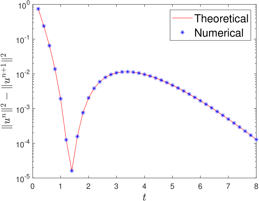
(a) Example 6.1

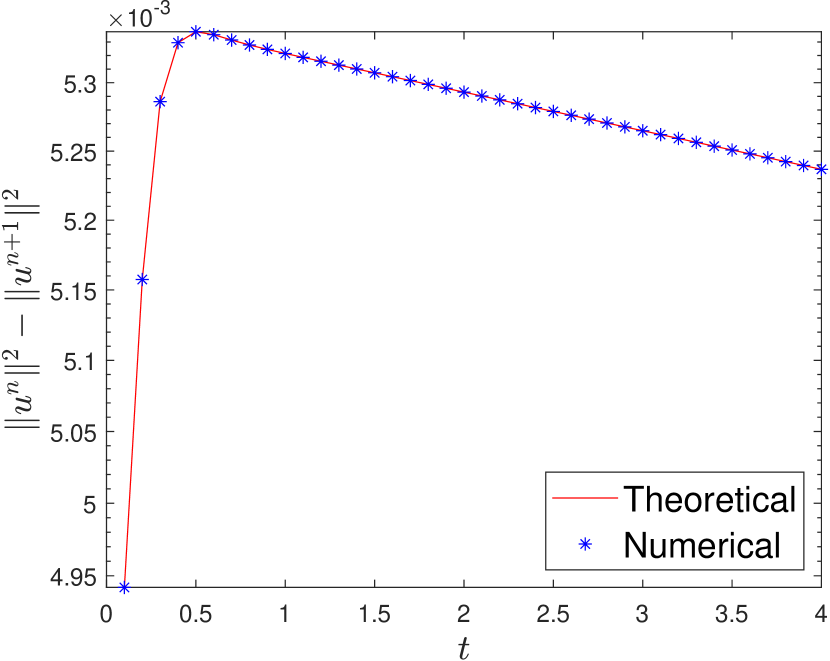
(b) Example 6.2

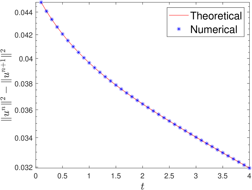
(c) Example 6.3

Figure 1: Numerical energy dissipation magnitudes and the theoretical ones given by the energy identity Eq. 32.

Example 6.3.

In this example, we study the following seminegative ODE system

(64) $$\frac{d}{dt}u=Lu,\quad u=u(t)\in L^{2}([0,T],\mathbb{R}^{N_{d}}),\quad L=\frac{1}{\Delta x^{3}}{\bf L}_{1}{\bf L}_{1}^{\top}{\bf L}_{1}^{\top}$$

with the matrix ${\bf L}_{1}$ defined by Eq. 63. This system comes from the piecewise constant (${\mathbb{P}}^{0}$-based) local discontinuous Galerkin discretization of the dispersion PDE $\psi_{t}+\psi_{xxx}=0$ in the spatial domain $[0,1]$ with the uniform mesh of $N_{d}=20$ cells (i.e., $\Delta x=1/N_{d}=0.05$) and periodic boundary conditions. The initial solution is taken as $\psi(x,0)=\cos(2\pi x)$. We solve the semi-discrete ODE system Eq. 64 in time up to $t=4$ by using the $(2,2)$ diagonal Padé approximation. The unconditional stability proved in Theorem 5.2 allows us to use a much larger time stepsize $\tau=0.1$, which is not restricted by the normal CFL condition $\Delta t\leq C\Delta x^{3}$ for an explicit time discretization such system Eq. 64. Fig. 1(c) displays the energy dissipation behavior, which is consistent with our theoretical analysis.

7 Conclusions

We have established a systematic theoretical framework to derive the discrete energy laws of general implicit and explicit Runge–Kutta (RK) methods for linear seminegative systems. The framework is motivated by a discrete analogue of integration by parts technique and a series expansion of the continuous energy law. The established discrete energy laws show a precise characterization on whether and how the energy dissipates in the RK discretization, thereby giving stability criteria of RK methods. We have also found a unified discrete energy law for all the diagonal Padé approximations, based on analytically constructing the Cholesky type decomposition of a class of symmetric matrices, whose structure is highly complicated. The discovery of the unified energy law and the proof of the decomposition are very nontrivial. For the diagonal Padé approximations, our analyses have bridged the continuous and discrete energy laws, enhancing our understanding of their intrinsic mechanisms. We have provided several specific examples of implicit methods to illustrate the discrete energy laws. A few numerical examples have also been given to confirm the theoretical properties. In this paper, we have developed new analysis techniques, with construction of technical combinatorial identities and the theory of hypergeometric series, which were rarely used in previous RK stability analyses and may motivate future developments in this field.

Appendix A Proof of Lemma 2.2

Proof A.1.

For any $v\in V$, we have

$$\sum_{i=0}^{N}\sum_{j=0}^{N}\gamma_{i,j}\tau^{i+j+1}\left[L^{i}v,L^{j}v\right]=-\sum_{i=0}^{N}\sum_{j=0}^{N}\left(\sum_{k=0}^{N}\mu_{k,i}d_{k}\mu_{k,j}\right)\tau^{i+j+1}\left[L^{i}v,L^{j}v\right]$$

$$= -\sum_{k=0}^{N}d_{k}\tau\left(\sum_{i=0}^{N}\sum_{j=0}^{N}\mu_{k,i}\mu_{k,j}\tau^{i+j}\left[L^{i}v,L^{j}v\right]\right)=-\sum_{k=0}^{N}d_{k}\tau\left[\sum_{i=k}^{N}\tau^{i}\mu_{k,i}L^{i}v,\sum_{j=k}^{N}\mu_{k,j}\tau^{j}L^{j}v\right]$$

$$= -\sum_{k=0}^{N}d_{k}\tau\left\llbracket\sum_{i=k}^{N}\tau^{j}\mu_{k,j}L^{j}v\right\rrbracket^{2}=-\sum_{k=0}^{N}d_{k}\tau^{2k+1}\left\llbracket L^{k}\left(\sum_{j=k}^{N}\mu_{k,j}(\tau L)^{j-k}\right)v\right\rrbracket^{2}.$$

Appendix B Proof of Lemma 2.3

Proof B.1.

Observe that $\boldsymbol{\widehat{\Upsilon}}=-\mathbf{D}_{0}\mathbf{H}\mathbf{D}_{0},$ where $\mathbf{D}_{0}=\operatorname{diag}(\{d_{i}\}_{i=0}^{N})$ with $d_{i}:=1/i!$, and $\mathbf{H}=(h_{i,j})_{i,j=0}^{N}$ is the Hilbert matrix with $h_{i,j}:={1}/{(i+j+1)}$. The Cholesky decomposition of the Hilbert matrix $\mathbf{H}$ gives $\mathbf{{H}}=\mathbf{{U}}_{H}^{\top}\mathbf{D}_{H}\mathbf{{U}}_{H},$ where the formulae of $\mathbf{U}_{H}$ and $\mathbf{D}_{H}$ were given in [17, Section 2] and also studied in [15, Lemma 2]. Therefore, we have

$$\boldsymbol{\widehat{\Upsilon}}=-\mathbf{D}_{0}\mathbf{U}_{H}^{\top}\mathbf{D}_{H}\mathbf{U}_{H}\mathbf{D}_{0}=-\left(\mathbf{D}_{0}^{-1}\mathbf{U}_{H}\mathbf{D}_{0}\right)^{\top}\left(\mathbf{D}_{0}\mathbf{D}_{H}\mathbf{D}_{0}\right)\left(\mathbf{D}_{0}^{-1}\mathbf{U}_{H}\mathbf{D}_{0}\right).$$

Taking $\mathbf{\widehat{U}}=\mathbf{D}_{0}^{-1}\mathbf{U}_{H}\mathbf{D}_{0}$ and $\mathbf{\widehat{D}}=\mathbf{D}_{0}\mathbf{D}_{H}\mathbf{D}_{0}$ with the formulae of $\mathbf{U}_{H}$ and $\mathbf{D}_{H}$ from [17, Section 2], we obtain Eq. 7 and complete the proof.

Appendix C Proof of Theorem 2.1

Proof C.1.

Because $\sum_{i=0}^{\infty}\left\|\frac{1}{i!}({\tau}L)^{i}u(t^{n})\right\|\leq\sum_{i=0}^{\infty}\frac{1}{i!}({\tau}\left\|L\right\|)^{i}\left\|u(t^{n})\right\|\leq e^{\tau\left\|L\right\|}\left\|u(t^{n})\right\|\leq e^{T\left\|L\right\|}\left\|u(t^{n})\right\|<\infty$, we known that the series $\sum_{i=0}^{\infty}\frac{1}{i!}({\tau}L)^{i}u(t^{n})$ converges. This implies that $v(t^{n}+\tau):=\sum_{i=0}^{\infty}\frac{1}{i!}({\tau}L)^{i}u(t^{n})$ is well-defined. We can verify that $\frac{d}{d\tau}v=Lv$. By the uniqueness of the solution to Eq. 1, we get $u(t^{n}+\tau)=v(t^{n}+\tau)=\sum_{i=0}^{\infty}\frac{1}{i!}({\tau}L)^{i}u(t^{n})$. Define $u_{N}(t^{n}+{\tau}):=\sum_{i=0}^{N}\frac{1}{i!}({\tau}L)^{i}u(t^{n}).$ As $N\to\infty$, we have $\left\|u_{N}-u\right\|\to 0$ and thus $\left\llbracket u_{N}\right\rrbracket\to\left\llbracket u\right\rrbracket$. It then follows from Eq. 4 that

(65) $$\left\|u(t^{n+1})\right\|^{2}-\left\|u(t^{n})\right\|^{2}=-\int_{0}^{\tau}\left\llbracket u(t^{n}+\widehat{\tau})\right\rrbracket^{2}\mathrm{d}\widehat{\tau}=-\int_{0}^{\tau}\lim_{N\to\infty}\left\llbracket u_{N}(t^{n}+\widehat{\tau})\right\rrbracket^{2}\mathrm{d}\widehat{\tau}.$$

Using the inequality $\left\llbracket u\right\rrbracket^{2}\leq 2\left\|L\right\|\left\|u\right\|^{2}$, we deduce that

(66) $$\left\llbracket u_{N}(t^{n}+\widehat{\tau})\right\rrbracket^{2}\leq 2\left\|L\right\|\left\|u_{N}(t^{n}+\widehat{\tau})\right\|^{2}\leq 2\left\|L\right\|\left(\sum_{i=0}^{N}\frac{1}{i!}\widehat{\tau}^{i}\left\|L\right\|^{i}\right)^{2}\left\|u(t^{n})\right\|^{2}\leq 2\left\|L\right\|e^{2\widehat{\tau}\left\|L\right\|}\left\|u(t^{n})\right\|^{2}.$$

Thanks to the dominated convergence theorem, the estimate Eq. 66 along with $\int_{0}^{\tau}2\left\|L\right\|e^{2\widehat{\tau}\left\|L\right\|}\left\|u(t^{n})\right\|^{2}\mathrm{d}\widehat{\tau}=(e^{2\tau\left\|L\right\|}-1)\left\|u(t^{n})\right\|^{2}<\infty$ implies $\int_{0}^{\tau}\lim_{N\to\infty}\left\llbracket u_{N}(t+\widehat{\tau})\right\rrbracket^{2}\mathrm{d}\widehat{\tau}=\lim_{N\to\infty}\int_{0}^{\tau}\left\llbracket u_{N}(t+\widehat{\tau})\right\rrbracket^{2}\mathrm{d}\widehat{\tau}.$ Combining it with Eq. 65 gives

(67) $$\left\|u(t^{n+1})\right\|^{2}-\left\|u(t^{n})\right\|^{2}=-\lim_{N\to\infty}\int_{0}^{\tau}\left\llbracket u_{N}(t+\widehat{\tau})\right\rrbracket^{2}\mathrm{d}\widehat{\tau}.$$

On the other hand, we can reformulate the integration Eq. 67 as follows

$$\int_{0}^{\tau}\left\llbracket u_{N}(t^{n}+\widehat{\tau})\right\rrbracket^{2}d\widehat{\tau} =\int_{0}^{\tau}\left[\sum_{i=0}^{N}\frac{1}{i!}(\widehat{\tau}L)^{i}u(t^{n}),\sum_{j=0}^{N}\frac{1}{j!}(\widehat{\tau}L)^{j}u(t^{n})\right]d\widehat{\tau}$$

$$=\sum_{i,j=0}^{N}\left(\int_{0}^{\tau}\frac{\widehat{\tau}^{i+j}}{i!j!}\mathrm{d}\widehat{\tau}\right)\left[L^{i}u(t^{n}),L^{j}u(t^{n})\right]$$

(68) $$=\sum_{i,j=0}^{N}\frac{\widehat{\tau}^{i+j+1}}{i!j!(i+j+1)}\left[L^{i}u(t^{n}),L^{j}u(t^{n})\right]=\sum_{k=0}^{N}\widehat{d}_{k}\tau^{2k+1}\left\llbracket L^{k}\widehat{u}_{N}^{(k)}\right\rrbracket^{2},$$

where the last equality follows from Lemmas 2.2 and 2.3, $\widehat{u}_{N}^{(k)}:=\sum_{j=k}^{N}\widehat{\mu}_{k,j}(\tau L)^{j-k}u(t^{n})$, and $\widehat{d}_{k}$ and $\widehat{\mu}_{k,j}$ are defined in (7). Hence, by combining Eq. 68 with Eq. 67, we obtain

(69) $$\left\|u(t^{n+1})\right\|^{2}-\left\|u(t^{n})\right\|^{2}=-\lim_{N\to\infty}\sum_{k=0}^{N}\widehat{d}_{k}\tau^{2k+1}\left\llbracket L^{k}\widehat{u}_{N}^{(k)}\right\rrbracket^{2}=-\lim_{N\to\infty}\sum_{k=0}^{\infty}\widehat{d}_{k}\tau^{2k+1}\left\llbracket L^{k}\widehat{u}_{N}^{(k)}\right\rrbracket^{2}1_{\{0,1,\dots,N\}}(k),$$

where $1_{\{0,1,\dots N\}}(\cdot)$ is the indicator function. Note that

(70) $$\widehat{d}_{k}\tau^{2k+1}\left\llbracket L^{k}\widehat{u}_{N}^{(k)}\right\rrbracket^{2}1_{\{0,1,\cdots,N\}}(k)\leq 2\tau\|L\|\|u(t^{n})\|^{2}\left(\sum_{j=k}^{N}\sqrt{\widehat{d}_{k}}\widehat{\mu}_{k,j}(\tau\|L\|)^{j}\right)^{2}=:{\mathcal{B}}_{k}.$$

The upper bound ${\mathcal{B}}_{k}$ satisfies

(71) $$\sum_{k=0}^{\infty}{\mathcal{B}}_{k}\leq\|u(t^{n})\|^{2}\left(e^{2\tau\|L\|}-1\right)<\infty,$$

because for any integer $M\geq N$,

$$\sum_{k=0}^{M}{\mathcal{B}}_{k} \leq 2\tau\|L\|\|u(t^{n})\|^{2}\sum_{k=0}^{M}\left(\sum_{j=k}^{M}\sqrt{\widehat{d}_{k}}\widehat{\mu}_{k,j}(\tau\|L\|)^{j}\right)^{2}$$

$$=2\tau\|L\|\|u(t^{n})\|^{2}\sum_{i=0}^{M}\sum_{j=0}^{M}\frac{(\tau\|L\|)^{i+j}}{i!j!(i+j+1)}=2\|u(t^{n})\|^{2}\int_{0}^{\tau\|L\|}\left(\sum_{i=0}^{M}\frac{x^{i}}{i!}\right)^{2}{\rm d}x$$

$$\leq 2\|u(t^{n})\|^{2}\int_{0}^{\tau\|L\|}e^{2x}{\rm d}x=\|u(t^{n})\|^{2}\left(e^{2\tau\|L\|}-1\right),$$

where we have used Lemma 2.3 in the first equality. Due to Eqs. 70 and 71, we can again invoke the dominated convergence theorem to exchange the limit and the infinite summation in Eq. 69 to obtain

$$\left\|u(t^{n+1})\right\|^{2}-\left\|u(t^{n})\right\|^{2}=-\sum_{k=0}^{\infty}\lim_{N\to\infty}\widehat{d}_{k}\tau^{2k+1}\left\llbracket L^{k}\widehat{u}_{N}^{(k)}\right\rrbracket^{2}1_{\{0,1,\cdots,N\}}(k)=-\sum_{k=0}^{\infty}\widehat{d}_{k}\tau^{2k+1}\left\llbracket L^{k}\widehat{u}^{(k)}\right\rrbracket^{2},$$

which completes the proof.

Appendix D Proof of Lemma 5.3

Proof D.1.

When $i>j$ or $i=j$, the identity is obviously true. In the following, we only focus on the case of $i<j$. Define

$$a_{\ell}:=\binom{s-\ell}{j-\ell}^{-1}\binom{2s-\ell}{j-i-\ell}\binom{i+j+1}{\ell}(-1)^{\ell}=\frac{(j-\ell)!(s-j)!(2s-\ell)!(i+j+1)!}{(s-\ell)!(j-i-\ell)!(2s-j+i)!\ell!(i+j+1-\ell)!}(-1)^{\ell}.$$

Then we have

$$a_{0}=\frac{j!(s-j)!(2s)!}{s!(j-i)!(2s-j+i)!},\qquad\frac{a_{\ell}}{a_{0}}=\prod_{k=0}^{\ell-1}\frac{a_{k+1}}{a_{k}}=\prod_{k=0}^{\ell-1}\left(\frac{(k-j+i)(k-s)(k-i-j-1)}{(k-2s)(k-j)}\frac{1}{k+1}\right).$$

Using the rising factorial notation Eq. 43, one can reformulate the sum in Lemma 5.3 as

(72) $$\sum_{\ell=0}^{j-i}a_{\ell}=a_{0}\sum_{\ell=0}^{j-i}\frac{(i-j)_{\ell}(-s)_{\ell}(-i-j-1)_{\ell}}{(-2s)_{\ell}(-j)_{\ell}}\frac{1}{\ell!}=a_{0}\sum_{\ell=0}^{\infty}\frac{(i-j)_{\ell}(-s)_{\ell}(-i-j-1)_{\ell}}{(-2s)_{\ell}(-j)_{\ell}}\frac{1}{\ell!},$$

where we have used the fact $(i-j)_{\ell}=0$ for $\ell>j-i$ and $\ell\in\mathbb{N}$. By using the notation ${}_{3}F_{2}{\left(\genfrac{.}{.}{0.0pt}{}{}{}\right)}$ from the theory of generalized hypergeometric functions [41], the above series can also be represented as

$$\sum_{\ell=0}^{\infty}\frac{(i-j)_{\ell}(-s)_{\ell}(-i-j-1)_{\ell}}{(-2s)_{\ell}(-j)_{\ell}}\frac{1}{\ell!}={}_{3}F_{2}{\left(\genfrac{.}{.}{0.0pt}{}{i-j{\mathchar 44\relax}\mskip 8.0mu-s{\mathchar 44\relax}\mskip 8.0mu-i-j-1}{-2s{\mathchar 44\relax}\mskip 8.0mu-j}\right)}={}_{3}F_{2}{\left(\genfrac{.}{.}{0.0pt}{}{-n{\mathchar 44\relax}\mskip 8.0muc{\mathchar 44\relax}\mskip 8.0mu2c+2d+n-1}{2c{\mathchar 44\relax}\mskip 8.0muc+d}\right)}$$

with $n:=j-i\in\mathbb{N}$, $c:=-s$, and $d:=s-j$. We use Watson’s formula [41] for such hypergeometric series:

(73) $${}_{3}F_{2}{\left(\genfrac{.}{.}{0.0pt}{}{-n{\mathchar 44\relax}\mskip 8.0muc{\mathchar 44\relax}\mskip 8.0mu2c+2d+n-1}{2c{\mathchar 44\relax}\mskip 8.0muc+d}\right)}=\begin{cases}\displaystyle\frac{n!\Gamma(c+\frac{1}{2}n)\Gamma(d+\frac{1}{2}n)\Gamma(2c)\Gamma(c+d)}{(\frac{1}{2}n)!\Gamma(c+d+\frac{1}{2}n)\Gamma(2c+n)\Gamma(c)\Gamma(d)},~{}&\mbox{if $n$ is even,}\\ 0,~{}&\mbox{if $n$ is odd.}\end{cases}$$

If $n=j-i$ is even, define $m:=\frac{j-i}{2}=\frac{1}{2}n\in\mathbb{N}$. Note that the singularity in Eq. 73 is removable, because

(74) $$\frac{\Gamma(x+m)}{\Gamma(x)}=\frac{(x+m-1)\Gamma(x+m-1)}{\Gamma(x)}=\dots=\prod_{\ell=0}^{m-1}(x+\ell)\neq 0,\qquad x=c,d,c+d,$$

(75) $$\frac{\Gamma(2c)}{\Gamma(2c+n)}=\frac{\Gamma(2c)}{(2c+n-1)\Gamma(2c+n-1)}=\dots=\prod_{\ell=0}^{n-1}\frac{1}{2c+\ell}=\frac{(2s-j+i)!}{(2s)!}>0,$$

where the formula $\Gamma(x+1)=x\Gamma(x)$ has been used repeatedly. It follows from Eq. 74 that

(76) $$\frac{\Gamma(c+\frac{1}{2}{n})}{\Gamma(c)}=\prod_{\ell=0}^{m-1}(-s+\ell)=(-1)^{m}\frac{s!}{(s-m)!}=(-1)^{m}\frac{s!}{(s-\frac{j-i}{2})!},$$

(77) $$\frac{\Gamma(d+\frac{1}{2}{n})}{\Gamma(d)}=\prod_{\ell=0}^{m-1}(s-j+\ell)=(s-j)\frac{(s-j+m-1)!}{(s-j)!}=(s-j)\frac{(s-1-\frac{i+j}{2})!}{(s-j)!},$$

(78) $$\frac{\Gamma(c+d)}{\Gamma(c+d+\frac{1}{2}n)}=(-1)^{m}\prod_{\ell=0}^{m-1}(j-\ell)^{-1}=(-1)^{m}\frac{(j-m)!}{j!}=(-1)^{m}\frac{(\frac{i+j}{2})!}{j!}.$$

Substituting Eq. 75–Eq. 78 into Eq. 73 and combining Eq. 72 with Eq. 73, we obtain for $i\equiv j~{}({\mathrm{mod}}~{}2)$ that

$$\sum_{\ell=0}^{j-i}a_{\ell}=a_{0}\frac{n!}{(\frac{1}{2}n)!}\frac{s!}{(s-\frac{j-i}{2})!}(s-j)\frac{(s-1-\frac{i+j}{2})!}{(s-j)!}\frac{(2s-j+i)!}{(2s)!}\frac{(\frac{i+j}{2})!}{j!}=\frac{(s-1-\frac{i+j}{2})!(\frac{i+j}{2})!}{(s-\frac{j-i}{2})!(\frac{j-i}{2})!}(s-j),$$

which completes the proof.

Appendix E Proof of Lemma 5.12

Proof E.1.

By the definition of the Pochhammer symbol, one can deduce that

$$(x+n)! =x!(x+1)(x+2)\cdots(x+n)=x!(x+1)_{n},$$

$$(x)_{n} =\left(\prod\limits_{0\leq 2i\leq n-1}(x+2i)\right)\cdot\left(\prod\limits_{0\leq 2i+1\leq n-1}(x+2i+1)\right)$$

$$=x(x+2)\cdots\left(x+2\left\lceil{\frac{n}{2}}\right\rceil-2\right)\cdot(x+1)(x+3)\cdots\left(x+2\left\lfloor{\frac{n}{2}}\right\rfloor-1\right)$$

$$=2^{\left\lceil{\frac{n}{2}}\right\rceil}\left(\frac{x}{2}\right)_{\left\lceil{\frac{n}{2}}\right\rceil}\cdot 2^{\left\lfloor{\frac{n}{2}}\right\rfloor}\left(\frac{x+1}{2}\right)_{\left\lfloor{\frac{n}{2}}\right\rfloor}=2^{n}\left(\frac{x}{2}\right)_{\left\lceil{\frac{n}{2}}\right\rceil}\left(\frac{x+1}{2}\right)_{\left\lfloor{\frac{n}{2}}\right\rfloor},$$

$$\frac{(x+i)!}{(x-j)!} =(x-j+1)(x-j+2)\cdots(x-1)x\cdot(x+1)\cdots(x+i)=(-1)^{j}(-x)_{j}(x+1)_{i}.$$

Appendix F Proof of Lemma 5.13

Proof F.1.

If $i>j$, then by definition (39) we know that $\nu_{2i,2j}^{(s)}=\nu_{2i-1,2j-1}^{(s)}=0$. On the other hand, when $i>j$, we have $(-j)_{i}=0$ and $(1-j)_{i-1}=0$, which imply the right-hand sides of (47) and (48) are both zero. Hence the identities (47) and (48) are true for $i>j$. In the following, we focus on the nontrivial case that $i\leq j$.

Proof of (47) for $i\leq j$. We observe that

$$\nu_{2i,2j}^{(s)} =\frac{s!}{(2s)!}\frac{2\sqrt{4i-1}}{(2i+2j)!}\frac{(2s+2i-2j)!(s-i-j)!(i+j)!}{(s-2j)!(s-j+i)!(j-i)!}=\frac{s!}{(2s)!}\frac{2\sqrt{4i-1}}{(s-2j)!}\Pi_{1}\Pi_{2}$$

with

$$\Pi_{1} :=\frac{(s-i-j)!}{(s-j+i)!}(2s-2j+2i)!\stackrel{{\scriptstyle\eqref{ID-1}}}{{=}}\frac{(s-j-i)!}{(s-j+i)!}(2s-2j)!(2s-2j+1)_{2i}$$

$$\stackrel{{\scriptstyle\eqref{ID-2}}}{{=}}\frac{(s-j-i)!}{(s-j+i)!}(2s-2j)!2^{2i}\left(s-j+\frac{1}{2}\right)_{i}(s-j+1)_{i}$$

$$\stackrel{{\scriptstyle\eqref{ID-3}}}{{=}}\frac{1}{(-1)^{i}(j-s)_{i}(s-j+1)_{i}}(2s-2j)!2^{2i}\left(s-j+\frac{1}{2}\right)_{i}(s-j+1)_{i}=\frac{(2s-2j)!2^{2i}\left(s-j+\frac{1}{2}\right)_{i}}{(j-s)_{i}(-1)^{i}},$$

and

$$\Pi_{2} :=\frac{(j+i)!}{(j-i)!}\frac{1}{(2i+2j)!}\stackrel{{\scriptstyle\eqref{ID-3}}}{{=}}\frac{(-1)^{i}(-j)_{i}(j+1)_{i}}{(2i+2j)!}\stackrel{{\scriptstyle\eqref{ID-1}}}{{=}}\frac{(-1)^{i}(-j)_{i}(j+1)_{i}}{(2j)!(2j+1)_{2i}}$$

$$\stackrel{{\scriptstyle\eqref{ID-2}}}{{=}}\frac{(-1)^{i}(-j)_{i}(j+1)_{i}}{(2j)!2^{2i}\left(j+\frac{1}{2}\right)_{i}(j+1)_{i}}=\frac{(-1)^{i}(-j)_{i}}{2^{2i}\left(j+\frac{1}{2}\right)_{i}}\frac{1}{(2j)!}.$$

It follows that

$$\Pi_{1}\Pi_{2}=\frac{(2s-2j)!}{(2j)!}\frac{\left(s-j+\frac{1}{2}\right)_{i}(-j)_{i}}{(j-s)_{i}\left(j+\frac{1}{2}\right)_{i}}.$$

Therefore, we obtain

$$\nu_{2i,2j}^{(s)} =2\sqrt{4i-1}\frac{s!}{(2s)!}\frac{(2s-2j)!}{(2j)!(s-2j)!}\frac{\left(s-j+\frac{1}{2}\right)_{i}(-j)_{i}}{(j-s)_{i}\left(j+\frac{1}{2}\right)_{i}}=2\sqrt{4i-1}\theta_{2j}^{(s)}\frac{\left(s-j+\frac{1}{2}\right)_{i}(-j)_{i}}{(j-s)_{i}\left(j+\frac{1}{2}\right)_{i}},$$

which yields (47).

Proof of (48) for $i\leq j$. We observe that

$$\nu_{2i-1,2j-1}^{(s)} =\frac{s!}{(2s)!}\frac{2\sqrt{4i-3}}{(2i+2j-2)!}\frac{(2s-2j+2i)!}{(s-j+i)!}\frac{(s-i-j+1)!}{(s-2j+1)!}\frac{(j+i-1)!}{(j-i)!}=\frac{s!}{(2s)!}\frac{2\sqrt{4i-3}}{(s-2j+1)!}\Pi_{3}\Pi_{4}$$

with

$$\Pi_{3} :=\frac{(s-i-j+1)!}{(s-j+i)!}(2s-2j+2i)!\stackrel{{\scriptstyle\eqref{ID-1}}}{{=}}\frac{(s-i-j+1)!}{(s-j+i)!}(2s-2j+1)!(2s-2j+2)_{2i-1}$$

$$\stackrel{{\scriptstyle\eqref{ID-2}}}{{=}}\frac{(s-i-j+1)!}{(s-j+i)!}(2s-2j+1)!2^{2i-1}(s-j+1)_{i}\left(s-j+\frac{3}{2}\right)_{i-1}$$

$$\stackrel{{\scriptstyle\eqref{ID-3}}}{{=}}\frac{(2s-2j+1)!}{(-1)^{i-1}(j-s)_{i-1}(s-j+1)_{i}}2^{2i-1}(s-j+1)_{i}\left(s-j+\frac{3}{2}\right)_{i-1}$$

$$=\frac{(2s-2j+1)!2^{2i-1}\left(s+\frac{3}{2}-j\right)_{i-1}}{(-1)^{i-1}(j-s)_{i-1}},$$

and

$$\Pi_{4} :=\frac{(j+i-1)!}{(j-i)!}\frac{1}{(2j+2i-2)!}\stackrel{{\scriptstyle\eqref{ID-3}}}{{=}}\frac{(-1)^{i}(-j)_{i}(j+1)_{i-1}}{(2j+2i-2)!}=\frac{(-1)^{i-1}(1-j)_{i-1}(j)_{i}}{(2j+2i-2)!}$$

$$\stackrel{{\scriptstyle\eqref{ID-1}}}{{=}}\frac{(-1)^{i-1}(1-j)_{i-1}(j)_{i}}{(2j-1)!(2j)_{2i-1}}\stackrel{{\scriptstyle\eqref{ID-2}}}{{=}}\frac{(-1)^{i-1}(1-j)_{i-1}(j)_{i}}{(2j-1)!2^{2i-1}(j)_{i}\left(j+\frac{1}{2}\right)_{i-1}}=\frac{(-1)^{i-1}(1-j)_{i-1}}{2^{2i-1}\left(j+\frac{1}{2}\right)_{i-1}}\frac{1}{(2j-1)!}.$$

It follows that

$$\Pi_{3}\Pi_{4}=\frac{(2s-2j+1)!}{(2j-1)!}\frac{\left(s+\frac{3}{2}-j\right)_{i-1}}{(j-s)_{i-1}}\frac{(1-j)_{i-1}}{\left(j+\frac{1}{2}\right)_{i-1}}.$$

Therefore, we complete the proof by noting

$$\nu_{2i-1,2j-1}^{(s)} =2\sqrt{4i-3}\frac{s!}{(2s)!}\frac{(2s-2j+1)!}{(2j-1)!(s-2j+1)!}\frac{\left(s+\frac{3}{2}-j\right)_{i-1}(1-j)_{i-1}}{(j-s)_{i-1}\left(j+\frac{1}{2}\right)_{i-1}}$$

$$=2\sqrt{4i-3}\theta_{2j-1}^{(s)}\frac{\left(s+\frac{3}{2}-j\right)_{i-1}(1-j)_{i-1}}{(j-s)_{i-1}\left(j+\frac{1}{2}\right)_{i-1}}.$$

References

- [1] G. Birkhoff and R. S. Varga, Discretization errors for well-set Cauchy problems, Journal of Mathematics and Physics, 44 (1965), p. 158.
- [2] C. Bresten, S. Gottlieb, Z. Grant, D. Higgs, D. Ketcheson, and A. Németh, Explicit strong stability preserving multistep Runge–Kutta methods, Math. Comp., 86 (2017), pp. 747–769.
- [3] E. Burman, A. Ern, and M. A. Fernández, Explicit Runge–Kutta schemes and finite elements with symmetric stabilization for first-order linear PDE systems, SIAM J. Numer. Anal., 48 (2010), pp. 2019–2042.
- [4] K. Burrage and J. C. Butcher, Stability criteria for implicit Runge–Kutta methods, SIAM J. Numer. Anal., 16 (1979), pp. 46–57.
- [5] J. C. Butcher, Numerical Methods for Ordinary Differential Equations, John Wiley & Sons, 2016.
- [6] B. Cockburn and C.-W. Shu, The local discontinuous Galerkin method for time-dependent convection-diffusion systems, SIAM J. Numer. Anal., 35 (1998), pp. 2440–2463.
- [7] G. G. Dahlquist, A special stability problem for linear multistep methods, BIT Numer. Math., 3 (1963), pp. 27–43.
- [8] E. Deriaz, Stability conditions for the numerical solution of convection-dominated problems with skew-symmetric discretizations, SIAM J. Numer. Anal., 50 (2012), pp. 1058–1085.
- [9] D. Drake, J. Gopalakrishnan, J. Schöberl, and C. Wintersteiger, Convergence analysis of some tent-based schemes for linear hyperbolic systems, arXiv preprint arXiv:2101.04798, (2021).
- [10] B. L. Ehle, A-stable methods and Padé approximations to the exponential, SIAM J. Math. Anal., 4 (1973), pp. 671–680.
- [11] B. L. Ehle and Z. Picel, Two-parameter, arbitrary order, exponential approximations for stiff equations, Math. Comp., 29 (1975), pp. 501–511.
- [12] J. Gopalakrishnan and Z. Sun, Stability of structure aware Taylor methods for tents, in preparation, (2022).
- [13] S. Gottlieb, C.-W. Shu, and E. Tadmor, Strong stability-preserving high-order time discretization methods, SIAM Rev., 43 (2001), pp. 89–112.
- [14] E. Hairer, G. Bader, and C. Lubich, On the stability of semi-implicit methods for ordinary differential equations, BIT Numer. Math., 22 (1982), pp. 211–232.
- [15] E. Hairer and G. Wanner, Algebraically stable and implementable Runge–Kutta methods of high order, SIAM J. Numer. Anal., 18 (1981), pp. 1098–1108.
- [16] I. Higueras, Monotonicity for Runge–Kutta methods: Inner product norms, J. Sci. Comput., 24 (2005), pp. 97–117.
- [17] S. Hitotumatu, Cholesky decomposition of the Hilbert matrix, Japan Journal of Applied Mathematics, 5 (1988), pp. 135–144.
- [18] A. Iserles, A First Course in the Numerical Analysis of Differential Equations, Cambridge University Press, 2009.
- [19] L. Isherwood, Z. J. Grant, and S. Gottlieb, Strong stability preserving integrating factor Runge–Kutta methods, SIAM J. Numer. Anal., 56 (2018), pp. 3276–3307.
- [20] D. I. Ketcheson, Relaxation Runge–Kutta methods: Conservation and stability for inner-product norms, SIAM J. Numer. Anal., 57 (2019), pp. 2850–2870.
- [21] D. I. Ketcheson, S. Gottlieb, and C. B. Macdonald, Strong stability preserving two-step Runge–Kutta methods, SIAM J. Numer. Anal., 49 (2011), pp. 2618–2639.
- [22] J. Kraaijevanger and M. Spijker, Algebraic stability and error propagation in Runge–Kutta methods, Appl. Numer. Math., 5 (1989), pp. 71–87.
- [23] J. F. B. M. Kraaijevanger, Contractivity of Runge–Kutta methods, BIT Numer. Math., 31 (1991), pp. 482–528.
- [24] D. Levy and E. Tadmor, From semidiscrete to fully discrete: Stability of Runge–Kutta schemes by the energy method, SIAM Rev., 40 (1998), pp. 40–73.
- [25] J. V. Neumann, Eine spektraltheorie für allgemeine operatoren eines unitären raumes, Mathematische Nachrichten, 4 (1950), pp. 258–281.
- [26] P. Öffner, J. Glaubitz, and H. Ranocha, Analysis of artificial dissipation of explicit and implicit time-integration methods, Int. J. Numer. Anal. Model., 17 (2020).
- [27] M. Qin and M. Zhang, Symplectic Runge–Kutta algorithms for Hamiltonian systems, J. Comput. Math., (1992), pp. 205–215.
- [28] H. Ranocha, On strong stability of explicit Runge–Kutta methods for nonlinear semibounded operators, IMA J. Numer. Anal., 41 (2021), pp. 654–682.
- [29] H. Ranocha and D. I. Ketcheson, Energy stability of explicit Runge–Kutta methods for nonautonomous or nonlinear problems, SIAM J. Numer. Anal., 58 (2020), pp. 3382–3405.
- [30] H. Ranocha and D. I. Ketcheson, Relaxation Runge–Kutta methods for Hamiltonian problems, J. Sci. Comput., 84 (2020), pp. 1–27.
- [31] H. Ranocha and P. Öffner, stability of explicit Runge–Kutta schemes, J. Sci. Comput., (2018), pp. 1–17.
- [32] H. Ranocha, M. Sayyari, L. Dalcin, M. Parsani, and D. I. Ketcheson, Relaxation Runge–Kutta methods: Fully discrete explicit entropy-stable schemes for the compressible Euler and Navier–Stokes equations, SIAM J. Sci. Comput., 42 (2020), pp. A612–A638.
- [33] M. Spijker, Contractivity in the numerical solution of initial value problems, Numer. Math., 42 (1983), pp. 271–290.
- [34] Z. Sun and C.-W. Shu, Stability of the fourth order Runge–Kutta method for time-dependent partial differential equations, Ann. Math. Sci. Appl., 2 (2017), pp. 255–284.
- [35] Z. Sun and C.-W. Shu, Strong stability of explicit Runge–Kutta time discretizations, SIAM J. Numer. Anal., 57 (2019), pp. 1158–1182.
- [36] Z. Sun and C.-W. Shu, Enforcing strong stability of explicit Runge–Kutta methods with superviscosity, Communications on Applied Mathematics and Computation, 3 (2021), pp. 671–700.
- [37] E. Tadmor, From semidiscrete to fully discrete: Stability of Runge–Kutta schemes by the energy method. II, Collected Lectures on the Preservation of Stability under Discretization, Lecture Notes from Colorado State University Conference, Fort Collins, CO, 2001 (D. Estep and S. Tavener, eds.), Proceedings in Applied Mathematics, SIAM, 109 (2002), pp. 25–49.
- [38] H. Wang, C.-W. Shu, and Q. Zhang, Stability and error estimates of local discontinuous Galerkin methods with implicit-explicit time-marching for advection-diffusion problems, SIAM J. Numer. Anal., 53 (2015), pp. 206–227.
- [39] G. Wanner and E. Hairer, Solving Ordinary Differential Equations II: Stiff and Difterential-Algebraic Problems, Springer Berlin Heidelberg, 1 ed., 1991.
- [40] G. Wanner, E. Hairer, and S. P. Nørsett, Order stars and stability theorems, BIT Numer. Math., 18 (1978), pp. 475–489.
- [41] G. N. Watson, A note on generalized hypergeometric series, Proc. London Math. Soc., s2-23 (1925), pp. xiii–xv.
- [42] Y. Xu, X. Meng, C.-W. Shu, and Q. Zhang, Superconvergence analysis of the Runge–Kutta discontinuous Galerkin methods for a linear hyperbolic equation, J. Sci. Comput., 84 (2020), pp. 1–40.
- [43] Y. Xu, Q. Zhang, C.-W. Shu, and H. Wang, The -norm stability analysis of Runge–Kutta discontinuous Galerkin methods for linear hyperbolic equations, SIAM J. Numer. Anal., 57 (2019), pp. 1574–1601.
- [44] Q. Zhang and C.-W. Shu, Stability analysis and a priori error estimates of the third order explicit Runge–Kutta discontinuous Galerkin method for scalar conservation laws, SIAM J. Numer. Anal., 48 (2010), pp. 1038–1063.