Model Aggregation for Risk Evaluation and Robust Optimization

Abstract

We introduce a new approach for prudent risk evaluation based on stochastic dominance, which will be called the model aggregation (MA) approach. In contrast to the classic worst-case risk (WR) approach, the MA approach produces not only a robust value of risk evaluation but also a robust distributional model, independent of any specific risk measure. The MA risk evaluation can be computed through explicit formulas in the lattice theory of stochastic dominance, and under some standard assumptions, the MA robust optimization admits a convex-program reformulation. The MA approach for Wasserstein and mean-variance uncertainty sets admits explicit formulas for the obtained robust models. Via an equivalence property between the MA and the WR approaches, new axiomatic characterizations are obtained for the Value-at-Risk (VaR) and the Expected Shortfall (ES, also known as CVaR). The new approach is illustrated with various risk measures and examples from portfolio optimization.

Keywords: Value-at-Risk, Expected Shortfall, stochastic dominance, model aggregation, worst-case risk measures, model uncertainty, robust optimization

1 Introduction

Modern risk management often requires the evaluation of risks under multiple scenarios. The risk evaluation obtained under various scenarios needs to be aggregated properly, and a prudent approach is often implemented in practice. As a prominent example, in the Fundamental Review of the Trading Book (FRTB) of Basel IV (BCBS (2019)), banks need to evaluate the market risk of their portfolio losses under stressed scenarios, in particular including a model generated from data during the financial crisis of 2007, and the obtained risk models are aggregated via a worst-case approach; see Wang and Ziegel (2021, Section 1) for a description of the stressed scenarios and the model aggregation in the FRTB, and Cambou and Filipović (2017) for techniques to generate regulatory scenarios. In the literature of portfolio risk assessment and optimization, the worst-case approach is popular; we refer to Ghaoui et al. (2003), Natarajan et al. (2008), Zhu and Fukushima (2009) and Glasserman and Xu (2014) for robust portfolio optimization, and Embrechts et al. (2013) and Wang et al. (2013) for robust risk aggregation. This idea further leads to many studies in distributionally robust optimization; see Delage and Ye (2010), Gao and Kleywegt (2016), Esfahani and Kuhn (2018) and Blanchet and Murthy (2019). In this paper, we will work in the context where a prudent risk evaluation under multiple models, which is our main focus, is desirable.

A natural question for risk management in the presence of model uncertainty is how to generate a robust model from a collection of models resulting from statistical and machine learning procedures, operational considerations, or expert’s opinion. Such a robust model can be used for risk evaluation, simulation, optimization, and decision making.

Our main ideas to address this question are described below. Let $\mathcal{M}$ be a set of distributions on $\mathbb{R}$, representing possible risk models; for illustrative purposes, we focus on one-dimensional financial losses for which the theory of risk measures is rich. Suppose that a risk analyst evaluates a random loss using different methodologies, scenarios or data sets, and obtains a collection $\mathcal{F}\subseteq\mathcal{M}$ of distributional models. Here, the number of models in $\mathcal{F}$ may be finite or infinite. For instance, $\mathcal{F}$ may contain distributions of the random loss under different probability measures (economic scenarios), estimation methods, or values of statistical parameters; alternatively, $\mathcal{F}$ may represent distributions from losses which may occur from different possible decisions from a business competitor. The set $\mathcal{F}$ will be called an uncertainty set. The distributions in $\mathcal{F}$ will be used to assess the risk, together with a risk measure $\rho:\mathcal{M}\to\mathbb{R}$, such as a Value-at-Risk (VaR) or an Expected Shortfall (ES, also known as CVaR); see Section 2.2 for their definitions. Prudent regulation and risk management require a conservative approach which aggregates the above information. There are two conceptually intuitive ways to generate a robust assessment of the risk:

1. Directly calculate the maximum (or supremum) of $\rho(F)$ over $F\in\mathcal{F}$.

2. Calibrate a robust (conservative) distributional model $F^{*}$ based on $\mathcal{F}$, and calculate $\rho(F^{*})$.

Arguably, each of (i) and (ii) is a reasonable approach to take, but they may yield different risk evaluations. We shall call (i) the worst-case risk (WR) approach, and (ii) the model aggregation (MA) approach. There are two obvious advantages of the MA approach: We obtain a robust model which is useful for analysis and simulation, thus answering the motivating question above, and the procedure applies for generic risk measures, not only a specific one. Other less obvious, but important, advantages of the MA approach will be revealed through this paper. The model $F^{*}$ is robust in two senses: First, it is more conservative than any models in $\mathcal{F}$; second, it applies to a wide range of risk measures or decision criteria.

At this point, we have not yet specified how the robust distributional model $F^{*}$ may be obtained in the MA approach (ii). For this purpose, we need an order relation, often consistent with the risk measure $\rho$ used by the risk analyst. We will describe some natural choices of partial orders, in particular, first- and second-order stochastic dominance, in Section 2.1.

Our main objective is a comprehensive theory on the two approaches of robust risk evaluation, with a focus on the newly introduced MA approach. The following questions naturally arise.

1. What are the advantages and disadvantages of the MA approach in contrast to the WR approach, in addition to the points mentioned above?

2. What are theoretical and computational properties of the MA approach in distributionally robust optimization?

3. Which risk measures yield equivalent robust risk evaluation results via the MA and WR approaches and how are they used in regulatory practice?

4. How is the MA approach implemented in common settings of uncertainty, optimization, and real-data applications?

We will answer the four questions above by means of several novel theoretical results. Our main contributions can be explained as follows. After introducing partial orders and risk measures in Section 2, we present a rigorous formulation of the MA and WR approaches for risk evaluation and robust optimization in Section 3. Our new method is related to stochastic optimization of risk measures (e.g., Dentcheva and Ruszczynski (2004), Ruszczyński and Shapiro (2006), Shapiro et al. (2021)); see our discussion in Section 3.

Features of MA risk evaluation will be discussed in Section 4 and MA robust optimization will be studied in Section 5. We show convenient properties of the MA approach in risk evaluation and optimization. In particular, the MA risk evaluation remains convex when the risk measure is convex, and the MA robust optimization admits a convex program reformulation under suitable conditions. This answers Q2, and also Q1 partially.

We establish in Section 7 that the property of equivalence in model aggregation characterizes VaR and ES among very general classes of risk measures. The equivalence property identifies for which risk measures the two approaches can be converted to each other. Through these results, which require long technical proofs, the rich literature of robust risk evaluation and optimization, popular in operations research, is connected to that of the axiomatic theory of risk preferences, popular in decision theory, for the first time. Our results contribute to the latter literature by offering new axiomatizations of both VaR and ES which are important issues in risk management in themselves. These results answer question Q3 above.

We address two settings of uncertainty, those generated by Wasserstein metrics and those generated by moment information in Section 6. We illustrate that the MA approach leads to closed-form robust distributional models in these settings, being easy to apply and computationally feasible. Based on a new result on dimension reduction for Wasserstein balls (Theorem 5), we show that the MA approach can conveniently handle multivariate Wasserstein uncertainty in the setting of portfolio selection. Section 8 contains two applications of worst-case risk evaluation and portfolio selection under uncertainty using real financial data. These two sections answer Q4.

Finally, advantages and limitations of the MA approach, as well as directions for future work, are summarized and discussed in Section 9, which also contains a preliminary discussion on aggregating multivariate risk models, in contrast to the univariate risk models treated throughout the paper. These discussions address Q1 at a high level.

In the main text of the paper, we focus on the set of distributions with finite mean to make our analysis concise and managerial insights clear. More general choices of the space of distributions are treated in the appendices, which also contain technical proofs of all results.

2 Preliminaries and standing notation

We first introduce some notation. Let $(\Omega,\mathcal{B},\mathbb{P})$ be a nonatomic probability space. For $d\in\mathbb{N}$, let $\mathfrak{B}(\mathbb{R}^{d})$ be the Borel $\sigma$-field on $\mathbb{R}^{d}$. A random vector $\mathbf{X}$ is a measurable mapping from $(\Omega,\mathcal{B})$ to $(\mathbb{R}^{d},\mathfrak{B}(\mathbb{R}^{d}))$. Denote by $\mu_{\mathbf{X}}:=\mathbb{P}\circ\mathbf{X}^{-1}$ the probability distribution induced by a random vector $\mathbf{X}$ under $\mathbb{P}$, where $\mathbf{X}^{-1}$ is the inverse image of $\mathbf{X}$. Denote by $F_{\mathbf{X}}$ the cumulative distribution function (cdf) of $\mathbf{X}$ under $\mathbb{P}$, i.e., $F_{\mathbf{X}}(\mathbf{x})=\mathbb{P}(\mathbf{X}\leqslant\mathbf{x})$ for $\mathbf{x}\in\mathbb{R}^{d}$, where the inequality is component-wise. We will take cdfs $F_{\mathbf{X}}$, identified with distributions $\mu_{\mathbf{X}}$, as the main research object of the entire paper. We use $\delta_{\mathbf{t}}$ to represent the point-mass at $\mathbf{t}\in\mathbb{R}^{d}$. Let $L^{1}$ be the space of all integrable random variables on $(\Omega,\mathcal{B},\mathbb{P})$, where almost surely equal random variables are treated as identical. Denote by $\mathcal{M}_{1}$ the set of cdfs of all random variables in $L^{1}$, i.e., $\mathcal{M}_{1}$ is the set of all cdfs $F$ satisfying $\int_{\mathbb{R}}|x|\mathrm{d}F(x)<\infty$. The mean of a random variable $X$ under $\mathbb{P}$ is written as $\mathbb{E}[X]=\mathfrak{m}(F_{X})$, where $\mathbb{E}$ is defined on $L^{1}$ and $\mathfrak{m}$ is defined on $\mathcal{M}_{1}$. We denote by $\Delta_{d}$ the standard simplex $\{\bm{\lambda}\in[0,1]^{d}:\sum_{i=1}^{d}\lambda_{i}=1\}$ in $\mathbb{R}^{d}$ and by $[d]=\{1,\dots,d\}$.

2.1 Stochastic orders and lattices

As mentioned in the introduction, to properly formulate the MA approach, a partial order $\preceq$ is needed on a set of cdfs, denoted by $\mathcal{M}$, and $(\mathcal{M},\preceq)$ is called a partially ordered set. The relevant tool is the lattice theory which we collect in Appendix B, and here we only present a basic result needed to understand our main ideas. The most commonly used partial orders in finance and economics are the first-order stochastic dominance $\preceq_{1}$ and the second-order stochastic dominance $\preceq_{2}$, defined as, for $F,G\in\mathcal{M}$,

1. $F\preceq_{1}G$ if $\int u\mathrm{d}F\leqslant\int u\mathrm{d}G$ for all increasing functions $u$;

2. $F\preceq_{2}G$ if $\int u\mathrm{d}F\leqslant\int u\mathrm{d}G$ for all increasing convex functions $u$.

Other useful equivalent definitions of $\preceq_{1}$ and $\preceq_{2}$ are put in Appendix B. To build a robust distributional model, we need to define the supremum of a set $\mathcal{F}$. The set $\mathcal{F}$ is always assumed to be nonempty. For an ordered set $(\mathcal{M},\preceq)$, the supremum of $\mathcal{F}$, denoted by $\bigvee\mathcal{F}$, is defined by $\bigvee\mathcal{F}\in\mathcal{M}$ and $F\preceq\bigvee\mathcal{F}\preceq G$ for all $F\in\mathcal{F}$ and all $G\in\mathcal{M}$ which dominates every element of $\mathcal{F}$ (uniqueness is guaranteed by definition). If such $G$ exists, we say that $\mathcal{F}$ is bounded from above with respect to $\preceq$, denoted by $\preceq$-bounded. The supremum does not always exist, but for the two choices of ordered sets $(\mathcal{M}_{1},\preceq_{1})$ and $(\mathcal{M}_{1},\preceq_{2})$ that we consider in the main paper, this does not create any problem; see e.g., Kertz and Rösler (2000) and Müller and Scarsini (2006) for the lattice structure of cdfs with $\preceq_{1}$ and $\preceq_{2}$. The two cases of $\bigvee\mathcal{F}$ for $\preceq_{1}$ and $\preceq_{2}$ admit explicit formulas, given in Proposition 1 in Section 4.

2.2 Risk measures

In the classic framework of Artzner et al. (1999) and Föllmer and Schied (2016), a risk measure is traditionally defined as a mapping from a set $\mathcal{X}$ of random losses to ${\mathbb{R}}$. Denote by $\mathcal{M}$ the set of cdfs of random variables in $\mathcal{X}$.

Definition 1.

A distribution based risk measure is a mapping $\rho:\mathcal{M}\to\mathbb{R}$. For such $\rho$, its associated random-variable based risk measure is $\widetilde{\rho}:\mathcal{X}\to\mathbb{R}$ given by $\widetilde{\rho}(X)=\rho(F_{X})$. Both $\rho$ and $\widetilde{\rho}$ will be called risk measures in this paper.

The random-variable based risk measure in Definition 1 satisfies law-invariance (i.e., $\widetilde{\rho}(X)=\widetilde{\rho}(Y)$ whenever $F_{X}=F_{Y}$). There exists a one-to-one correspondence between $\rho:\mathcal{M}\to\mathbb{R}$ and $\phi:\mathcal{X}\to\mathbb{R}$ satisfying law-invariance; see e.g., Proposition 1 of Delage et al. (2019). We will choose $\mathcal{X}=L^{1}$ in the main part of the paper, so that the two partial orders $\preceq_{1}$ and $\preceq_{2}$ both behave well. For a better exposition of distributional uncertainty, we will present ideas and results mainly using $\rho$ instead of $\widetilde{\rho}$.

The two most popular and important risk measures in financial practice, VaR and ES, are both law-invariant. The risk measure VaR at level $\alpha\in(0,1)$ is the functional $\mathrm{VaR}_{\alpha}:\mathcal{M}_{1}\to\mathbb{R}$ defined by

$$\mathrm{VaR}_{\alpha}(F)=\inf\{x\in\mathbb{R}:F(x)\geqslant\alpha\},$$

which is the left $\alpha$-quantile of a cdf. The risk measure ES at level $\alpha\in[0,1)$ is the functional $\mathrm{ES}_{\alpha}:\mathcal{M}_{1}\to\mathbb{R}$ defined by

$$\mathrm{ES}_{\alpha}(F)=\frac{1}{1-\alpha}\int_{\alpha}^{1}{\rm VaR}_{s}(F)\mathrm{d}s,$$

and in particular, $\mathrm{ES}_{0}(F)=\mathfrak{m}(F)$. We can also define $\mathrm{VaR}_{0}$, $\mathrm{VaR}_{1}$ and $\mathrm{ES}_{1}$ which are not finite-valued on $\mathcal{M}_{1}$; see Appendix C.

For a partial order $\preceq$ on $\mathcal{M}$, a natural interpretation of $F\preceq G$ is that $G$ is riskier than $F$ according to $\preceq$. A risk measure $\rho:\mathcal{M}\to\mathbb{R}$ is $\preceq$-consistent if $\rho(F)\leqslant\rho(G)$ for all $F,G\in\mathcal{M}$ with $F\preceq G$. Note that $\rho$ is $\preceq_{1}$-consistent if and only if $\widetilde{\rho}$ is monotone (i.e., $\widetilde{\rho}(X)\leqslant\widetilde{\rho}(Y)$ when $X\leqslant Y$). Hence, all commonly used risk measures, including VaR, are $\preceq_{1}$-consistent. Moreover, ES satisfies both $\preceq_{1}$ and $\preceq_{2}$-consistency. Throughout the paper, we assume risk measures are $\preceq_{1}$-consistent.

3 Introducing the MA approach

We describe the two approaches for robust risk evaluation, the primary objects of this paper. For a risk measure $\rho:\mathcal{M}\to\mathbb{R}$ and an uncertainty set $\mathcal{F}\subseteq\mathcal{M}$, a common way to obtain a robust risk evaluation is to calculate the following worst-case risk measure

$${\rm WR:}~{}~{}~{}~{}~{}\rho^{\rm WR}(\mathcal{F})=\sup_{F\in\mathcal{F}}\rho(F).$$ (1)

The value in (1) is called the WR robust $\rho$ value, and it has been widely studied in the literature; some references are mentioned in the introduction. Next, we propose a new method of robust risk evaluation, that is, assuming that the supremum $\bigvee\mathcal{F}$ with respect to $\preceq$ exists,

$${\rm MA:}~{}~{}~{}~{}~{}\rho^{\rm MA}(\mathcal{F})=\rho\left(\bigvee\mathcal{F}\right),$$ (2)

and $\rho^{\rm MA}(\mathcal{F})=\infty$ if $\mathcal{F}$ is not bounded from above. The value in (2) is called the $\preceq$-MA robust $\rho$ value (“$\preceq$-” will be omitted if the order is clear from the context). In the main text of the paper, $\bigvee\mathcal{F}$ exists for all $\mathcal{F}$ bounded from above, and hence, $\rho^{\rm MA}$ is always well-defined. In case that $\bigvee\mathcal{F}$ may not exist, (2) needs to be modified as in Appendix B.

The idea of the MA approach can be described in two steps: First, take the supremum $\bigvee\mathcal{F}$ of the uncertainty set $\mathcal{F}$ as the robust distribution, and second, calculate the value of the risk measure of the robust distribution. The robust distribution $\bigvee\mathcal{F}$ obtained in the first step can be used for any risk measure. If, in addition, the risk measure $\rho$ is $\preceq$-consistent, then the MA approach produces a larger robust risk value than the WR approach, that is, for any $\mathcal{F}\subseteq\mathcal{M}$,

$$\rho^{\rm WR}(\mathcal{F})\leqslant\rho^{\rm MA}(\mathcal{F}),$$ (3)

since $\preceq$-consistency implies $\rho(\bigvee\mathcal{F})\geqslant\rho(F)$ for all $F\in\mathcal{F}$. The MA approach can be implemented even in case no risk measure is involved (thus skipping the second step above), as the model $\bigvee\mathcal{F}$ is ready to use without a specification of any specific objective.

In the sequel, we will focus on $\preceq_{1}$ and $\preceq_{2}$. For a simpler notation, we write ${\rm MA}_{1}$ when $\preceq$ is specified as $\preceq_{1}$, and ${\rm MA}_{2}$ is similar. For these two stochastic orders, the explicit forms of $\bigvee\mathcal{F}$ are obtained in Section 4. It is also worth noting that if $\rho$ is consistent with more than one partial orders, then the MA approach with a stronger partial order leads to a higher risk evaluation. For instance, if $\rho$ is both $\preceq_{1}$-consistent and $\preceq_{2}$-consistent, then $\rho^{\rm WR}(\mathcal{F})\leqslant\rho^{{\rm MA}_{2}}(\mathcal{F})\leqslant\rho^{{\rm MA}_{1}}(\mathcal{F})$ because any $(\mathcal{M},\preceq_{1})$-upper bound on $\mathcal{F}$ is also an $(\mathcal{M},\preceq_{2})$-upper bound on $\mathcal{F}$.

Using the WR and MA approaches, two types of robust optimization problems arise:

$$\min_{\mathbf{a}\in A}~{}~{}\rho^{\rm WR}(\mathcal{F}_{\mathbf{a},f})\mbox{~{}~{}~{}~{}~{}and~{}~{}~{}~{}~{}}\min_{\mathbf{a}\in A}~{}~{}\rho^{\rm MA}(\mathcal{F}_{\mathbf{a},f}),$$ (4)

where $A$ is a set of possible actions, $f:A\times\mathbb{R}^{d}\to\mathbb{R}$ is a loss function, $\mathcal{F}$ is a set of cdfs on $\mathbb{R}^{d}$ and

$$\mathcal{F}_{\mathbf{a},f}=\left\{F_{f(\mathbf{a},\mathbf{X})}:F_{\mathbf{X}}\in\mathcal{F}\right\}.$$ (5)

The set $\mathcal{F}_{\mathbf{a},f}$ consists all univariate cdfs of $f(\mathbf{a},\mathbf{X})$ where $\mathbf{X}$ has cdf in $\mathcal{F}$. For instance, by choosing $A\subseteq\mathbb{R}^{d}$ and $f(\mathbf{a},\mathbf{x})=\mathbf{a}^{\top}\mathbf{x}$, one arrives at the setting of robust portfolio selection, where $\mathbf{a}$ represents the vector of portfolio weights and $\mathbf{x}$ represents the vector of losses from individual assets. The WR robust optimization problem in (4) is equivalent to a minimax problem:

$$\min_{\mathbf{a}\in A}~{}\sup_{F\in\mathcal{F}}\widetilde{\rho}^{F}(f(\mathbf{a},\mathbf{X})),$$ (6)

where $\widetilde{\rho}^{F}(f(\mathbf{a},\mathbf{X}))$ represents the value of $\widetilde{\rho}(f(\mathbf{a},\mathbf{X}))$ when $\mathbf{X}$ has the cdf $F$. If $\rho$ is $\preceq$-consistent, then the MA robust optimization problem in (4) can be converted to a stochastic program with partial order $\preceq$ constraints:

$$\min_{\mathbf{a}\in A}~{}\inf_{H}\rho(H)~{}~{}~{}~{}~{}~{}{\rm s.t.}~{}G\preceq H,~{}~{}\forall G\in\mathcal{F}_{\mathbf{a},f}.$$ (7)

The above problem with $\preceq$ being $\preceq_{2}$ will be studied in Section 5. Section 6 is dedicated to the portfolio selection problem, where two specific settings of uncertainty will be considered.

Comparison: Optimization with stochastic dominance. Dentcheva and Ruszczynski (2004) introduced an optimization problem with stochastic dominance constraint. Adapting to our notation, and focusing on $\preceq_{2}$, their model can be described as

$$\min_{\mathbf{a}\in A}~{}~{}\mathbb{E}[f(\mathbf{a},\mathbf{X})]~{}~{}~{}~{}~{}~{}{\rm s.t.}~{}F_{g_{i}(\mathbf{a},\mathbf{X})}\preceq_{2}F_{i},~{}~{}i\in[m],$$ (8)

where $\mathbf{X}$ has a fixed cdf, $f,g_{1},\dots,g_{m}$ are fixed functions, and $F_{1},\dots,F_{m}\in\mathcal{M}_{1}$. Note that if we replace $\mathbb{E}$ by $\widetilde{\rho}$ and set $g_{1}=\dots=g_{m}=f$, then the problem is

$$\min_{\mathbf{a}\in A}~{}~{}\widetilde{\rho}(f(\mathbf{a},\mathbf{X}))~{}~{}~{}~{}~{}~{}{\rm s.t.}~{}F_{f(\mathbf{a},\mathbf{X})}\preceq_{2}F_{i},~{}~{}i\in[m].$$ (9)

The problem (9) is similar to our MA problem (7), but there are a few essential differences. First, for fixed $\mathbf{a}\in A$, the cdf of ${f(\mathbf{a},\mathbf{X})}$ is fixed in (9), whereas (7) searches for a robust model for $f(\mathbf{a},\mathbf{X})$ over the uncertainty set $\mathcal{F}_{\mathbf{a},f}$. Second, the direction of stochastic dominance is flipped, as our $H$ dominates every $G$ in $\mathcal{F}_{\mathbf{a},f}$ and their $F_{f(\mathbf{a},\mathbf{X})}$ is dominated by every $F_{i}$. Note that the interpretation of stochastic dominance is very different here: (7) looks at risks larger in $\preceq_{2}$ (riskier) because our objective is robust optimization, whereas (9) looks at risks smaller in $\preceq_{2}$ (safer) because of risk constraint. In Dentcheva and Ruszczynski (2003), the following problem has been considered: $\min_{X\in\mathcal{C}}\widetilde{\rho}(X)~{}{\rm s.t.}~{}F_{X}\preceq_{2}F_{i},~{}i\in[m],$ where $\mathcal{C}$ is a set of random variables. When $\rho$ is $\preceq_{2}$-consistent, our MA risk evaluation problem can be written as $\min_{X\in L^{1}}\widetilde{\rho}(X)~{}{\rm s.t.}~{}F_{i}\preceq_{2}F_{X},~{}i\in[m],$ which is similar to the model of Dentcheva and Ruszczynski (2003); see the recent work of Dentcheva (2023) for a related two-stage optimization with stochastic dominance constraints.

Remark 1.

In this paper, we focus on risk measures taking real values. In some applications, risk measures may be multi-valued or set-valued (e.g., Embrechts and Puccetti (2006), Hamel and Heyde (2010), Hamel et al. (2011)). For such risk measures, the MA approach, together with multivariate stochastic order, can also be applied.

4 MA approach in risk evaluation

In this section, we study properties of the MA risk evaluation by focusing on $\preceq_{1}$ and $\preceq_{2}$.

4.1 Computing the robust model

We use $\bigvee_{1}\mathcal{F}$ and $\bigvee_{2}\mathcal{F}$ to represent the supremum of the uncertainty set $\mathcal{F}$ on the ordered set $(\mathcal{M}_{1},\preceq_{1})$ and $(\mathcal{M}_{1},\preceq_{2})$, respectively, and $\pi_{F_{X}}$ represents the integrated survival function of $X\in L^{1}$, defined as

$$\pi_{F_{X}}(x)=\int_{x}^{\infty}(1-F_{X}(t)){\mathrm{d}}t=\mathbb{E}[(X-x)_{+}],~{}~{}~{}x\in\mathbb{R},$$ (10)

where $x_{+}=\max\{0,x\}$ for $x\in\mathbb{R}$. It is straightforward from (10) that a simple relationship between the integrated survival function $\pi_{F}$ and the cdf $F$ is $F=1+(\pi_{F})_{+}^{\prime}$, where $(\pi_{F})_{+}^{\prime}$ is the right derivative of $\pi_{F}$. The left quantile function of $F\in\mathcal{M}_{1}$ is defined by $F^{-1}(\alpha)=\inf\{x\in\mathbb{R}:F(x)\geqslant\alpha\}$ for $\alpha\in(0,1]$, which is $\mathrm{VaR}_{\alpha}(F)$ when $\alpha\in(0,1)$. The functions $\pi_{F}$ and $F^{-1}$ will be used throughout the paper.

Proposition 1.

• For a set $\mathcal{F}\subseteq\mathcal{M}_{1}$ which is $\preceq_{1}$-bounded, we have $\bigvee_{1}\mathcal{F}=\inf_{F\in\mathcal{F}}F$ and the left quantile function of $\bigvee_{1}\mathcal{F}$ is $\sup_{F\in\mathcal{F}}F^{-1}$.

• For a set $\mathcal{F}\subseteq\mathcal{M}_{1}$ which is $\preceq_{2}$-bounded, we have

  $$\pi_{\bigvee_{2}\mathcal{F}}=\sup_{F\in\mathcal{F}}\pi_{F},\mbox{~{}and thus~{}}\bigvee_{2}\mathcal{F}=1+\left(\sup_{F\in\mathcal{F}}\pi_{F}\right)_{+}^{\prime}.$$ (11)

By Proposition 1, optimization of $\mathrm{MA}_{1}$ leads to the worst-case quantile optimization; see e.g., Ghaoui et al. (2003). Similarly, optimization of $\mathrm{MA}_{2}$ leads to the worst-case first upper partial moment optimization, which also has wide range of applications; see Lo (1987), Natarajan et al. (2010) and Cowell (2011). To compute $\pi_{\bigvee_{2}\mathcal{F}}$ numerically, as a decreasing convex function, $\pi_{\bigvee_{2}\mathcal{F}}$ can be well approximated by a piece-wise linear function with finitely many pieces (which requires computing it at finitely many points). The next result concerns convexity of the uncertainty set.

Proposition 2.

Suppose that $i\in\{1,2\}$. For $\mathcal{F}\subseteq\mathcal{M}_{1}$, we have $\bigvee_{i}{\rm conv}{\mathcal{F}}=\bigvee_{i}\mathcal{F}$, where ${\rm conv}{\mathcal{F}}$ is the convex hull of $\mathcal{F}$.

Proposition 2 illustrates that for the ${\rm MA}_{1}$ and ${\rm MA}_{2}$ approaches, one can convert freely between any uncertainty set and its convex hull. For WR risk evaluation, this does not hold in general.

4.2 VaR and ES

Next we discuss the MA and WR approaches applied to VaR and ES, and this will help us understand the inequality (3). The case of VaR, coupled with the partial order $\preceq_{1}$, is simple. By Proposition 1, for $\alpha\in(0,1)$ and any $\mathcal{F}$ that is $\preceq_{1}$-bounded, $\mathrm{VaR}_{\alpha}^{\rm WR}(\mathcal{F})=\mathrm{VaR}_{\alpha}^{{\rm MA}_{1}}(\mathcal{F})$, and thus (3) holds as an equality in this specific setting; this result will be collected in Theorem 1 below.

The case of ES is more illuminating. Note that ES is consistent with respect to both $\preceq_{1}$ and $\preceq_{2}$. First, we consider the MA approach with $\preceq_{1}$. Since

$$\mathrm{ES}_{\alpha}^{\rm WR}(\mathcal{F})=\frac{1}{1-\alpha}\sup_{F\in\mathcal{F}}\int_{\alpha}^{1}F^{-1}(s)\mathrm{d}s\leqslant\frac{1}{1-\alpha}\int_{\alpha}^{1}\sup_{F\in\mathcal{F}}F^{-1}(s)\mathrm{d}s=\mathrm{ES}_{\alpha}^{{\rm MA}_{1}}(\mathcal{F}),$$

for (3) to hold as an equality, one needs to exchange the order of a supremum and an integral. Such an exchange, if legitimate, means that there exists $F\in\mathcal{F}$ such that $F^{-1}(s)\geqslant G^{-1}(s)$ for all $G\in\mathcal{F}$ and $s\in(\alpha,1)$, which is a quite strong assumption unlikely to hold in applications.

Next, we consider the MA approach for ES with $\preceq_{2}$. Recall a representation of $\mathrm{ES}_{\alpha}$ for $\alpha\in(0,1)$ in the celebrated work of Rockafellar and Uryasev (2002), that is,

$$\mathrm{ES}_{\alpha}(F)=\min_{x\in\mathbb{R}}\left\{x+\frac{1}{1-\alpha}\pi_{F}(x)\right\},~{}~{}~{}F\in\mathcal{M}_{1}.$$ (12)

Using (12), we obtain the WR robust ES value, that is,

$$\mathrm{ES}_{\alpha}^{\rm WR}(\mathcal{F})=\sup_{F\in\mathcal{F}}\mathrm{ES}_{\alpha}(F) =\sup_{F\in\mathcal{F}}\min_{x\in\mathbb{R}}\left\{x+\frac{1}{1-\alpha}\pi_{F}(x)\right\}.$$ (13)

On the other hand, the $\preceq_{2}$-MA robust ES value can also be calculated using (12) and (11) in Proposition 1, that is,

$$\mathrm{ES}_{\alpha}^{{\rm MA}_{2}}(\mathcal{F})=\mathrm{ES}_{\alpha}\left(\bigvee_{2}\mathcal{F}\right) =\min_{x\in\mathbb{R}}\sup_{F\in\mathcal{F}}\left\{x+\frac{1}{1-\alpha}\pi_{F}(x)\right\},$$ (14)

where the second equality follows from (12) and $\pi_{\bigvee_{2}\mathcal{F}}(x)=\sup_{F\in\mathcal{F}}\pi_{F}(x)$ by Proposition 1 (ii). The formulas (13) and (14) imply that the WR and MA robust ES values can be seen as, respectively, the maximin and the minimax of the same bivariate objective function. This observation immediately leads to

$$\mathrm{ES}_{\alpha}^{\rm WR}(\mathcal{F})\leqslant\mathrm{ES}_{\alpha}^{{\rm MA}_{2}}(\mathcal{F}),\mbox{ and equality holds if a minimax theorem holds}.$$ (15)

Therefore, although (3) is generally not an equality, it may be an equality for $\mathrm{ES}_{\alpha}$ and $\preceq_{2}$ under certain conditions on $\mathcal{F}$. In particular, as shown by Zhu and Fukushima (2009), if $\mathcal{F}$ is a convex polytope (see Section 7 for a definition) or a compact convex set of discrete cdfs, then (15) becomes an equality. In the following theorem, we establish a more general sufficient condition to make (15) an equality, where $\mathrm{ES}_{0}=\mathfrak{m}$ and $\mathrm{ES}_{\alpha}$ for $\alpha\in(0,1)$ are treated separately. We also collect the corresponding result for $\mathrm{VaR}_{\alpha}$ discussed above.

Theorem 1.

Suppose that $\mathcal{F}\subseteq\mathcal{M}_{1}$.

• If $\sup_{F\in\mathcal{F}}\int_{\mathbb{R}}(x-y)_{+}\mathrm{d}F(y)\to 0$ as $x\to-\infty$, then $\mathfrak{m}^{\rm WR}(\mathcal{F})=\mathfrak{m}^{{\rm MA}_{2}}(\mathcal{F})$.

• For $\alpha\in(0,1)$, if $\mathcal{F}$ is convex and $\preceq_{2}$-bounded, then $\mathrm{ES}_{\alpha}^{\rm WR}(\mathcal{F})=\mathrm{ES}_{\alpha}^{{\rm MA}_{2}}(\mathcal{F})$.

• For $\alpha\in(0,1)$, if $\mathcal{F}$ is $\preceq_{1}$-bounded, then $\mathrm{VaR}_{\alpha}^{\rm WR}(\mathcal{F})=\mathrm{VaR}_{\alpha}^{{\rm MA}_{1}}(\mathcal{F})$.

The most useful part of Theorem 1 is (b), which offers a simple condition under which the WR robust ES value can be obtained by implementing the MA approach. This result generalizes Theorems 1 and 2 of Zhu and Fukushima (2009) where the set $\mathcal{F}$ is a convex polytope and a compact convex set of discrete cdfs, respectively. Without convexity of $\mathcal{F}$, for $\alpha\in(0,1)$, $\mathrm{ES}_{\alpha}^{\rm WR}(\mathcal{F})=\mathrm{ES}_{\alpha}^{{\rm MA}_{2}}(\mathcal{F})$ may not hold, as illustrated by the following example.

Example 1.

Let $\alpha\in(0,1)$. Let $\varepsilon=(1-\alpha)/2$, $F_{1}=\delta_{0}$ and $F_{2}=(1-\varepsilon)\delta_{-1/(1-\varepsilon)-1}+\varepsilon\delta_{1/\varepsilon}$, where $\delta_{t}$ represents the point-mass at $t\in\mathbb{R}$. By computing $\max\{\pi_{F_{1}},\pi_{F_{2}}\}$, we get $\bigvee_{2}\{F_{1},F_{2}\}=(1-\varepsilon)\delta_{-1/(1-\varepsilon)}+\varepsilon\delta_{1/\varepsilon}$ and

$$\mathrm{ES}_{\alpha}\left(\bigvee_{2}\{F_{1},F_{2}\}\right)=\frac{1}{2}\left(\frac{1}{\varepsilon}-\frac{1}{1-\varepsilon}\right)>\frac{1}{2}\left(\frac{1}{\varepsilon}-\frac{2-\varepsilon}{1-\varepsilon}\right)_{+}=\max\left\{\mathrm{ES}_{\alpha}(F_{1}),\mathrm{ES}_{\alpha}(F_{2})\right\}.$$

Hence, $\mathrm{ES}_{\alpha}^{\rm WR}(\{F_{1},F_{2}\})<\mathrm{ES}_{\alpha}^{{\rm MA}_{2}}(\{F_{1},F_{2}\})$.

The conditions on $\mathcal{F}$ in (a) and (b) of Theorem 1 do not imply each other. The following example shows that $\mathfrak{m}^{\rm WR}(\mathcal{F})=\mathfrak{m}^{{\rm MA}_{2}}(\mathcal{F})$ may not hold in case $\mathcal{F}$ does not satisfy the condition in (a) and satisfy the condition in (b).

Example 2.

For $n\in\mathbb{N}$, let $F_{n}=(1/n)\delta_{-n}+(1-1/n)\delta_{0}$, and denote by $\mathcal{F}$ the convex hull of $\{F_{n}\}_{n\in\mathbb{N}}$. By computing $\max\{\pi_{F_{n}},n\in\mathbb{N}\}$, we have $\bigvee_{2}\mathcal{F}=\bigvee_{2}\{F_{n}\}_{n\in\mathbb{N}}=\delta_{0}$. Note that $\mathfrak{m}(F)=-1$ for any $F\in\mathcal{F}$. Hence, $\mathfrak{m}(\bigvee_{2}\mathcal{F})=0>-1=\sup_{F\in\mathcal{F}}\mathfrak{m}(F)$, that is, $\mathfrak{m}^{\rm WR}(\mathcal{F})<\mathfrak{m}^{{\rm MA}_{2}}(\mathcal{F})$.

4.3 Convexity and other properties

We first introduce some standard properties of a risk measure $\rho:\mathcal{M}_{1}\to\mathbb{R}$ and its associated $\widetilde{\rho}:L^{1}\to\mathbb{R}$. Translation invariance: $\widetilde{\rho}(X+c)=\widetilde{\rho}(X)+c$ for any $c\in\mathbb{R}$ and $X\in L^{1}$. Positive homogeneity: $\widetilde{\rho}({\lambda X})=\lambda\widetilde{\rho}(X)$ for any $\lambda>0$ and $X\in L^{1}$. Convexity: $\widetilde{\rho}({\lambda X+(1-\lambda)Y})\leqslant\lambda\widetilde{\rho}(X)+(1-\lambda)\widetilde{\rho}(Y)$ for any $\lambda\in[0,1]$ and $X,Y\in L^{1}$. Lower semicontinuity: $\liminf_{n\to\infty}\widetilde{\rho}(X_{n})\geqslant\widetilde{\rho}(X)$ if $X_{n},X\in L^{1}$ for all $n$ and $X_{n}\stackrel{{\scriptstyle\rm d}}{{\to}}X$ as $n\to\infty$, where $\stackrel{{\scriptstyle\rm d}}{{\to}}$ denotes convergence in distribution. Comonotonic additivity: $\widetilde{\rho}({X+Y})=\widetilde{\rho}(X)+\widetilde{\rho}(Y)$ for any $X,Y\in L^{1}$ that are comonotonic. A risk measure is coherent, as defined by Artzner et al. (1999), if it satisfies translation invariance, positive homogeneity, and convexity. All the properties are defined for both $\rho$ and $\widetilde{\rho}$.

It is well known that $\mathrm{VaR}_{\alpha}$ and $\mathrm{ES}_{\alpha}$, $\alpha\in(0,1)$ satisfy translation invariance, positive homogeneity, lower semicontinuity, comonotonic additivity, and $\mathrm{ES}_{\alpha}$ further satisfies convexity. Translation invariance, positive homogeneity and convexity are standard properties with interpretations extensively discussed by Artzner et al. (1999) and Föllmer and Schied (2016). Lower semicontinuity, called the prudence axiom by Wang and Zitikis (2021), means that if the loss cdf is modeled using a truthful approximation, then the approximated risk model should not underreport the capital requirement. Comonotonic additivity is popular in both the literature of decision theory (e.g., Yaari (1987) and Schmeidler (1989)) and that of risk measures (e.g., Kusuoka (2001)). A coherent risk measure on $\mathcal{M}_{1}$, including ES, is automatically consistent with both $\preceq_{1}$ and $\preceq_{2}$; see e.g., Föllmer and Schied (2016) and Shapiro et al. (2021).

Next we formulate uncertainty for $\widetilde{\rho}$ with different probabilities based on $\rho:\mathcal{M}_{1}\to\mathbb{R}$. Let $\mathcal{P}$ be the set of all probability measures on $(\Omega,\mathcal{B})$ absolutely continuous with respect to $\mathbb{P}$. Define $\widetilde{\rho}^{Q}(X)=\rho(F_{X}^{Q})$ where $F_{X}^{Q}$ is denoted by the cdf of $X$ under $Q\in\mathcal{P}$, assumed to be in $\mathcal{M}_{1}$. In particular, we have $\widetilde{\rho}^{\mathbb{P}}(X)=\widetilde{\rho}(X)=\rho(F_{X})$ for all $X\in L^{1}$. For $\mathcal{Q}\subseteq\mathcal{P}$, we use $\mathcal{F}_{X|\mathcal{Q}}$ to represent the set of all possible cdfs of $X$ under the uncertainty set, i.e., $\mathcal{F}_{X|\mathcal{Q}}=\{F_{X}^{Q}:Q\in\mathcal{Q}\}$.

In this setting, we study the properties of risk measures via WR approach

$${\rm WR:}~{}~{}~{}~{}~{}\widetilde{\rho}^{\rm WR}(X)=\rho^{\rm WR}\left(\mathcal{F}_{X|\mathcal{Q}}\right)=\sup_{F\in\mathcal{F}_{X|\mathcal{Q}}}\rho(F)=\sup_{Q\in\mathcal{Q}}\widetilde{\rho}^{Q}(X),$$

and via ${\rm MA}_{i}$ approach for $i=1,2$,

$${\rm MA:}~{}~{}~{}~{}~{}\widetilde{\rho}^{{\rm MA}_{i}}(X)=\rho^{{\rm MA}_{i}}\left(\mathcal{F}_{X|\mathcal{Q}}\right)=\rho\left(\bigvee_{i}{\mathcal{F}_{X|\mathcal{Q}}}\right),~{}~{}i=1,2.$$

The two mappings $\widetilde{\rho}^{{\rm WR}}$ and $\widetilde{\rho}^{{\rm MA}_{i}}$ are well defined on the set $L=\bigcap_{Q\in\mathcal{Q}}L^{1}(\Omega,\mathcal{B},Q)$. This set always contains, for instance, all bounded random variables in $L^{1}$. The next result gives properties of $\widetilde{\rho}^{{\rm WR}}$ and $\widetilde{\rho}^{{\rm MA}_{i}}$ based on those of $\widetilde{\rho}$.

Theorem 2.

Let $\widetilde{\rho}:L^{1}\to\mathbb{R}$ be a risk measure, $\mathcal{Q}\subseteq\mathcal{P}$, and $L=\bigcap_{Q\in\mathcal{Q}}L^{1}(\Omega,\mathcal{B},Q)$. The following statements hold.

• If $\widetilde{\rho}$ is convex, then $\widetilde{\rho}^{\rm WR}$ and $\widetilde{\rho}^{{\rm MA}_{2}}$ are convex on $L$.

• If $\widetilde{\rho}$ satisfies comonotonic additivity, then $\widetilde{\rho}^{{\rm MA}_{1}}$ satisfies comonotonic additivity on $L$.

• If $\widetilde{\rho}$ satisfies translation invariance (positive homogeneity), then $\widetilde{\rho}^{\rm WR}$, $\widetilde{\rho}^{{\rm MA}_{1}}$ and $\widetilde{\rho}^{{\rm MA}_{2}}$ satisfy translation invariance (positive homogeneity) on $L$.

A direct result from Theorem 2 is that $\widetilde{\rho}^{\rm WR}$ and $\widetilde{\rho}^{{\rm MA}_{2}}$ are coherent whenever $\widetilde{\rho}$ is a coherent risk measure. Note that $\widetilde{\rho}^{\rm WR}$ may not be comonotonic additive even if $\widetilde{\rho}$ is. For instance, the mapping $\widetilde{\rho}^{\rm WR}:X\mapsto\max\{\mathbb{E}^{\mathbb{P}_{1}}[X],\mathbb{E}^{\mathbb{P}_{2}}[X]\}$ for $\mathbb{P}_{1}\neq\mathbb{P}_{2}$ is not comonotonic additive in general.

Remark 2.

Although all the risk measures considered in the paper are law-invariant with respect to $\mathbb{P}$, $\widetilde{\rho}^{\rm WR}$, $\widetilde{\rho}^{{\rm MA}_{1}}$ and $\widetilde{\rho}^{{\rm MA}_{2}}$ may not be law-invariant with respect to any one probability measure. Nevertheless, $\widetilde{\rho}^{\rm WR}$, $\widetilde{\rho}^{{\rm MA}_{1}}$ and $\widetilde{\rho}^{{\rm MA}_{2}}$ are all law-invariant with respect to the probability set $\mathcal{Q}$ according to the definitions of Delage et al. (2019) and Wang and Ziegel (2021).

5 MA approach in robust optimization

In this section, we consider general robust optimization problems where uncertainty is addressed by the WR and ${\rm MA}_{2}$ approaches, i.e., $\preceq_{2}$ is chosen as the partial order. Let $A$ be a set of possible actions, $f:A\times\mathbb{R}^{d}\to\mathbb{R}$ be a loss function, $\mathcal{F}$ be a set of cdfs on $\mathbb{R}^{d}$, and $\mathcal{F}_{\mathbf{a},f}$ is defined by (5). We consider the following two optimization problems

$$\min_{\mathbf{a}\in A}~{}~{}\rho^{\rm WR}(\mathcal{F}_{\mathbf{a},f})\mbox{~{}~{}~{}~{}~{}and~{}~{}~{}~{}~{}}\min_{\mathbf{a}\in A}~{}~{}\rho^{{\rm MA}_{2}}(\mathcal{F}_{\mathbf{a},f}).$$ (16)

Recall the equivalency between the WR robust optimization and (6), i.e., $\min_{\mathbf{a}\in A}\rho^{\rm WR}(\mathcal{F}_{\mathbf{a},f})=\min_{\mathbf{a}\in A}\sup_{F\in\mathcal{F}}\widetilde{\rho}^{F}(f(\mathbf{a},\mathbf{X}))$. It is straightforward to see that the WR robust optimization is a convex problem if $A$, $\rho$ and $f$ (in its first argument) are convex as the inner problem is the supremum of a set of convex functionals. We demonstrate in the following result that the ${\rm MA}_{2}$ robust optimization is convex under the same conditions.

Proposition 3.

Let $A$ be a convex set. Suppose that a risk measure $\rho:\mathcal{M}_{1}\to\mathbb{R}$ is convex, and $f:A\times\mathbb{R}^{d}\to\mathbb{R}$ is convex in its first argument. Then, the mapping $\mathbf{a}\mapsto\rho^{\rm MA_{2}}(\mathcal{F}_{\mathbf{a},f})$ is convex. As a consequence, the ${\rm MA}_{2}$ robust optimization problem in (16) is a convex optimization problem.

We note that the convexity of both WR and ${\rm MA}_{2}$ robust optimization problems may not always coincide; see Appendix D.2.

Next, we detail the application of the ${\rm MA}_{2}$ approach to a broad class of coherent risk measures. We introduce an extra assumption before diving in.

Assumption 1.

For any $\mathbf{a}\in A$, the uncertainty set $\mathcal{F}_{\mathbf{a},f}$ is $\preceq_{2}$-bounded.

Assumption 1 guarantees that $\bigvee_{2}\mathcal{F}_{\mathbf{a},f}$ exists for any $\mathbf{a}\in A$. This assumption is mild. For example, it holds if we consider a common compact support of all involved cdfs.

A law-invariant coherent risk measure has a Kusuoka representation (Kusuoka (2001) and Shapiro (2013)), which can be approximated by the following form

$$\rho(F)=\sup_{w\in\mathbb{W}}~{}\sum_{j=1}^{n^{w}}p_{j}^{w}{\rm ES}_{\alpha_{j}^{w}}(F),$$ (17)

where $\mathbb{W}$ is a finite index set, and for each $w\in\mathbb{W}$, $n^{w}\in\mathbb{N}$, $(p_{1}^{w},\dots,p_{n^{w}}^{w})\in\Delta_{n^{w}}$ and $(\alpha_{1}^{w},\dots,\alpha_{n^{w}}^{w})\in[0,1]^{n^{w}}$. For the risk measure in (17), we obtain a reformulation of the ${\rm MA}_{2}$ robust optimization.

Theorem 3.

Suppose that Assumption 1 holds, and let $\rho$ be given by (17). The ${\rm MA}_{2}$ robust optimization problem in (16) can be reformulated as the following problem

$$\min_{\mathbf{a}\in A,\,x_{j}^{w},h,h_{j}^{w}\in\mathbb{R}}~{} h$$ (18)

$${\rm s.t.}~{}~{} \sum_{j=1}^{n^{w}}p_{j}^{w}h_{j}^{w}\leqslant h,~{}~{}w\in\mathbb{W}$$

$$x_{j}^{w}+\frac{1}{1-\alpha_{j}^{w}}\sup_{F\in\mathcal{F}}\mathbb{E}^{F}[(f({\bf a},\mathbf{X})-x_{j}^{w})_{+}]\leqslant h_{j}^{w},~{}~{}j\in[n^{w}],~{}w\in\mathbb{W}.$$

Consider a finite uncertainty set $\mathcal{F}=\{F_{1},\dots,F_{n}\}$, where $n\in\mathbb{N}$. Under this setting, we reformulate the ${\rm MA}_{2}$ robust optimization which is a direct consequence of Theorem 3. The two optimization problems in (16) can be respectively reformed as

$$\mbox{$\mathrm{WR}$}:\min_{\mathbf{a}\in A,\,x_{i,j}^{w},h,h_{i,j}^{w}\in\mathbb{R}}~{} h$$ (19)

$${\rm s.t.}~{}~{} \sum_{j=1}^{n^{w}}p_{j}^{w}h_{i,j}^{w}\leqslant h,~{}~{}i\in[n],~{}w\in\mathbb{W}$$

$$x_{i,j}^{w}+\frac{1}{1-\alpha_{j}^{w}}\mathbb{E}^{F_{i}}[(f(\mathbf{a},\mathbf{X})-x_{i,j}^{w})_{+}]\leqslant h_{i,j}^{w},~{}~{}i\in[n],~{}j\in[n^{w}],~{}w\in\mathbb{W};$$

$$\mbox{$\mathrm{MA}_{2}$}:\min_{\mathbf{a}\in A,\,x_{j}^{w},h,h_{j}^{w}\in\mathbb{R}}~{} h$$ (20)

$${\rm s.t.}~{}~{} \sum_{j=1}^{n^{w}}p_{j}^{w}h_{j}^{w}\leqslant h,~{}~{}w\in\mathbb{W}$$

$$x_{j}^{w}+\frac{1}{1-\alpha_{j}^{w}}\mathbb{E}^{F_{i}}[(f(\mathbf{a},\mathbf{X})-x_{j}^{w})_{+}]\leqslant h_{j}^{w},~{}~{}i\in[n],~{}j\in[n^{w}],~{}w\in\mathbb{W}.$$

If $\rho=\mathrm{ES}_{\alpha}$ for $\alpha\in(0,1)$, then the two optimization problems in (16) can be reformed as

$$\mbox{$\mathrm{WR}$}:\min_{\mathbf{a}\in A,\,x_{i},h\in\mathbb{R}}~{}h~{}~{}~{}~{}{\rm s.t.}~{}~{}x_{i}+\frac{1}{1-\alpha}\mathbb{E}^{F_{i}}[(f(\mathbf{a},\mathbf{X})-x_{i})_{+}]\leqslant h,~{}i\in[n];$$

$$\mbox{$\mathrm{MA}_{2}$}:\min_{\mathbf{a}\in A,\,x,h\in\mathbb{R}}~{}h~{}~{}~{}~{}{\rm s.t.}~{}~{}x+\frac{1}{1-\alpha}\mathbb{E}^{F_{i}}[(f(\mathbf{a},\mathbf{X})-x)_{+}]\leqslant h,~{}i\in[n].$$

Remark 3.

By Theorem 3 (or using Proposition 2), the ${\rm MA}_{2}$ robust optimization retains the form (20) if we substitute the uncertainty set $\mathcal{F}=\{F_{1},\dots,F_{n}\}$ with any set $\widetilde{\mathcal{F}}$, whose convex hull has extreme points $F_{1},\ldots,F_{n}$.

For other settings of Problem (18) that are solvable by convex program, see Appendix D.2. The two optimization problems in (16) are equivalent under a convex uncertainty set $\mathcal{F}$ when $\rho={\rm ES}_{\alpha}$ for all $\alpha\in(0,1)$. This equivalence stems from the fact that $\mathcal{F}_{\mathbf{a},f}$ is convex for all $\mathbf{a}\in A$ which combining with Theorem 1 imply $\mathrm{ES}_{\alpha}^{\rm WR}(\mathcal{F}_{\mathbf{a},f})=\mathrm{ES}_{\alpha}^{\rm MA_{2}}(\mathcal{F}_{\mathbf{a},f})$ for all $\mathbf{a}\in A$. Many results in the literature rely on converting between $\mathrm{ES}_{\alpha}^{\rm WR}(\mathcal{F}_{\mathbf{a},f})$ and $\mathrm{ES}_{\alpha}^{\rm MA_{2}}(\mathcal{F}_{\mathbf{a},f})$; see e.g., Zhu and Fukushima (2009), Natarajan et al. (2010) and Cowell (2011).

To compare the tractability of (19) and (20), set

$$f({\bf a},{\bf x})=\sum_{i=1}^{d}[\beta_{i}(a_{i}-x_{i})_{+}+\eta_{i}(x_{i}-a_{i})_{+}],$$

where $\beta_{i},\eta_{i}\in\mathbb{R}_{+}$. This is the loss function of the newsvendor problem. Take $F_{i}={\rm N}({\bm{\mu}}_{i},\Sigma_{i})$ for $i\in[n]$. We generate the parameters by $({\bm{\mu}}_{i},\bm{\sigma}_{i})\stackrel{{\scriptstyle{\rm i.i.d.}}}{{\sim}}{\rm N}_{2d}(0,I_{2d})~{}\mbox{and}~{}\Sigma_{i}=\mathrm{diag}(\exp(\bm{\sigma}_{i}))\mbox{~{}for $i\in[n]$},$ where $I_{d}$ is the $d\times d$ identity matrix and $\exp$ is applied component-wise. Similarly to Rockafellar and Uryasev (2002), we use a Monte Carlo simulation to approximate the term $x+\mathbb{E}^{F_{i}}[(f(\mathbf{a},\mathbf{X})-x)_{+}]/(1-\alpha)$ for $x\in\mathbb{R}$, $\alpha\in[0,1)$ and $i\in[n]$. Figure 1 presents the computation times of two approaches where we use the cvxpy library with MOSEK as the chosen solver. The corresponding parameters are summarized below. We set $\beta_{i}=i$ and $\eta_{i}=d-i+1$ for $i\in[d]$. We assume that the values of $n^{w}$ are identical for all $w\in\mathbb{W}$, and $p_{j}^{w}$, $j\in[n^{w}]$ are uniformly generated from the standard $n^{w}$-simplex, and $\alpha_{j}^{w}=(2j-1)/(2n^{w})$ for $j\in[n^{w}]$. Each panel in Figure 1 illustrates the performance as one parameter varies, while the other parameters are held constant at $(n^{w},d,n,|\mathbb{W}|,N)=(10,3,3,3,100)$. As shown in Figure 1, the computation times of the two approaches appear to be similar for most values of $d$, $n$ and $N$. In the case of large $n^{w}$ or large $|\mathbb{W}|$, the MA approach is visibly faster. This is consistent with our intuition that MA may work better when the risk measure itself is more complicated.

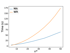
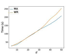
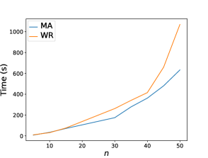
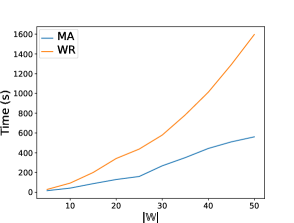
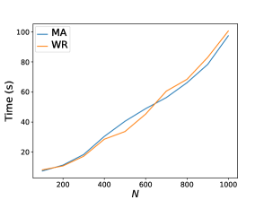
Figure 1: Computation times of MA and WR methods

Note: $d$ is the dimension of the random vector; $n$ is the number of cdfs in $\mathcal{F}$; $|\mathbb{W}|$ is the cardinality of $\mathbb{W}$; $N$ is the sample size drawn from each $F_{i}\in\mathcal{F}$. We assume that $n^{w}$ is identical for each $w\in\mathbb{W}$.

6 Wasserstein and mean-variance uncertainty sets

In this section, we focus on three specific and popular uncertainty sets: (a) univariate Wasserstein uncertainty, (b) multivariate Wasserstein uncertainty, and (c) mean-variance uncertainty. We obtain explicit formulas for the robust models as well as the WR and MA robust risk evaluation. Furthermore, the portfolio selection problem will be explored based on these two robust approaches.

For results in this section and Section 8, we define a few classes of risk measures other than $\mathrm{VaR}$ and $\mathrm{ES}$. The Range Value-at-Risk (RVaR), proposed by Cont et al. (2010), is defined as

$${\rm RVaR}_{\alpha,\beta}(F)=\frac{1}{\beta-\alpha}\int_{\alpha}^{\beta}\mathrm{VaR}_{s}(F)\mathrm{d}s,~{}~{}0\leqslant\alpha<\beta\leqslant 1.$$

Special and limiting cases of ${\rm RVaR}_{\alpha,\beta}$ include $\mathrm{ES}_{\alpha}$ with $\beta=1$ and $\mathrm{VaR}_{\beta}$ with $\alpha\uparrow\beta\in(0,1)$. If $\beta<1$, then ${\rm RVaR}_{\alpha,\beta}$ is not $\preceq_{2}$-consistent by e.g., Wang et al. (2020, Theorem 3). The power-distorted (PD) risk measure (Wang (1995); Cherny and Madan (2009)) is defined as

$${\rm PD}_{k}(F)=\int_{0}^{1}ks^{k-1}\mathrm{VaR}_{s}(F)\mathrm{d}s,~{}~{}k\geqslant 1.$$

The PD risk measure is coherent. The expectile, proposed by Newey and Powell (1987) and denoted by $\mathrm{ex}_{\alpha}$, is defined as the unique solution $t=\mathrm{ex}_{\alpha}(F_{X})\in\mathbb{R}$ to the following equation,

$$\alpha\mathbb{E}[(X-t)_{+}]=(1-\alpha)\mathbb{E}[(X-t)_{-}],~{}~{}X\in L^{1}.$$

The risk measure $\mathrm{ex}_{\alpha}$ is coherent (and thus $\preceq_{2}$-consistent) if and only if $\alpha\in[1/2,1)$; we will use this specification.

6.1 Uncertainty induced by the univariate Wasserstein metric

We first focus on an uncertainty set induced by the Wasserstein metric. Let $\mathcal{M}_{p}$ be the set of cdfs on $\mathbb{R}$ with finite $p$th moment and $F_{0}\in\mathcal{M}_{p}$ be a pre-specified cdf used as benchmark. For $p\geqslant 1$, the $p$-Wasserstein metric between $F$ and $F_{0}$ is defined as

$${W_{p}}(F,F_{0})=\left(\int_{0}^{1}|F^{-1}(s)-F_{0}^{-1}(s)|^{p}\mathrm{d}s\right)^{1/p}.$$ (21)

The corresponding uncertainty set is, for a parameter $\varepsilon\geqslant 0$,

$$\mathcal{F}_{p,\varepsilon}(F_{0})=\left\{F\in\mathcal{M}_{p}:W_{p}(F,F_{0})\leqslant\varepsilon\right\},$$ (22)

which is a convex set. The parameter $\varepsilon$ represents the magnitude of uncertainty. Denote by

$$F_{p,\varepsilon|F_{0}}^{1}=\bigvee_{1}\mathcal{F}_{p,\varepsilon}(F_{0})~{}~{}~{}{\rm and}~{}~{}~{}F_{p,\varepsilon|F_{0}}^{2}=\bigvee_{2}\mathcal{F}_{p,\varepsilon}(F_{0})$$

the supremum of $\mathcal{F}_{p,\varepsilon}(F_{0})$ with respect to $\preceq_{1}$ and $\preceq_{2}$, respectively. In the following result, we will identify an explicit form of the suprema $F_{p,\varepsilon|F_{0}}^{1}$ and $F_{p,\varepsilon|F_{0}}^{2}$ in terms of left quantile functions.

Theorem 4.

Suppose that $\varepsilon>0$, $p\geqslant 1$ and $F_{0}\in\mathcal{M}_{p}$.

• The left quantile function of $F_{p,\varepsilon|F_{0}}^{1}$ is uniquely determined by

  $$\int_{\alpha}^{1}\left((F_{p,\varepsilon|F_{0}}^{1})^{-1}(\alpha)-F_{0}^{-1}(s)\right)_{+}^{p}\mathrm{d}s=\varepsilon^{p},~{}~{}~{}\alpha\in(0,1).$$ (23)

• The set $\mathcal{F}_{1,\varepsilon}(F_{0})$ is not $\preceq_{2}$-bounded. For $p>1$, the left quantile function of $F_{p,\varepsilon|F_{0}}^{2}$ is given by

  $$(F_{p,\varepsilon|F_{0}}^{2})^{-1}(\alpha)=F_{0}^{-1}(\alpha)+\left(1-\frac{1}{p}\right)(1-\alpha)^{-1/p}\varepsilon,~{}~{}~{}\alpha\in(0,1).$$ (24)

Since the cdfs $F_{p,\varepsilon|F_{0}}^{1}$ and $F_{p,\varepsilon|F_{0}}^{2}$, as well as their quantile functions, are obtained explicitly in Theorem 4, the robust risk values $\rho^{{\rm MA}_{1}}(\mathcal{F}_{p,\varepsilon}(F_{0}))$ and $\rho^{{\rm MA}_{2}}(\mathcal{F}_{p,\varepsilon}(F_{0}))$ can be computed in a straightforward manner. On the other hand, $\rho^{\rm WR}(\mathcal{F}_{p,\varepsilon}(F_{0}))$ is often difficult to compute if the risk measure is complicated, although there are some results in the literature that considered the WR approach for special choices of risk measures. Postek et al. (2016) presented combinations of risk measures and uncertainty sets that allow for computationally tractable reformulations.

As a feature of the robust model, both $F_{p,\varepsilon|F_{0}}^{1}$ and $F_{p,\varepsilon|F_{0}}^{2}$ are heavy-tailed even if the benchmark distribution $F_{0}$ is light-tailed. Heavy-tailed distributions are common for modeling financial data; see e.g., McNeil et al. (2015). Indeed, $(F_{p,\varepsilon|F_{0}}^{1})^{-1}\geqslant(F_{p,\varepsilon|F_{0}}^{2})^{-1}$, and $(F_{p,\varepsilon|F_{0}}^{2})^{-1}$ is the sum of the quantile $F_{0}^{-1}$ and a Pareto quantile with tail index $p>1$. Some other observations on the supremum distributions in Theorem 4 are made in Remark EC.2.

Noting that the Wasserstein uncertainty set $\mathcal{F}_{p,\varepsilon}(F_{0})$ is convex, we have $\mathrm{ES}_{\alpha}^{\rm WR}(\mathcal{F}_{p,\varepsilon}(F_{0}))=\mathrm{ES}_{\alpha}^{{\rm MA}_{2}}(\mathcal{F}_{p,\varepsilon}(F_{0}))$ by Theorem 1. A simulation result in case of $p=2$, $\varepsilon=0.1$ and a standard normal benchmark distribution is reported in Appendix E.2.

6.2 Multivariate Wasserstein uncertainty

For $p\geqslant 1$ and $a\geqslant 1$, let $\mathcal{M}_{p}(\mathbb{R}^{d})$ be the set of all cdfs on $\mathbb{R}^{d}$ with finite $p$th moment in each component. The $p$-Wasserstein metric on $\mathbb{R}^{d}$ between $F,G\in\mathcal{M}_{p}(\mathbb{R}^{d})$ is defined as

$${W^{d}_{a,p}}(F,G)=\inf_{F_{\mathbf{X}}=F,F_{\mathbf{Y}}=G}\left(\mathbb{E}[\|\mathbf{X}-\mathbf{Y}\|^{p}_{a}]\right)^{1/p},$$

where $\|\cdot\|_{a}$ is the $L^{a}$ norm on $\mathbb{R}^{d}$; see e.g., Blanchet et al. (2022). If $d=1$, then $W_{a,p}^{d}$ is $W_{p}$ in (21) where the infimum is attained by comonotonicity via the Fréchet-Hoeffding inequality. Define the Wasserstein uncertainty set for a benchmark distribution $F_{0}\in\mathcal{M}_{p}(\mathbb{R}^{d})$ as, similar to (22),

$$\mathcal{F}_{a,p,\varepsilon}^{d}(F_{0})=\left\{F\in\mathcal{M}_{p}(\mathbb{R}^{d}):W^{d}_{a,p}(F,F_{0})\leqslant\varepsilon\right\},~{}~{}\varepsilon\geqslant 0.$$ (25)

We focus on a portfolio selection problem, i.e., the loss function is chosen as the linear function $f(\mathbf{w},\mathbf{x})=\mathbf{w}^{\top}\mathbf{x}$. The portfolio risk is $\rho(F_{\mathbf{w}^{\top}\mathbf{X}})$ for some weight vector $\mathbf{w}\in\mathbb{R}^{d}$ and risk vector $\mathbf{X}$ with unknown cdf in the multi-dimensional Wasserstein ball $\mathcal{F}_{a,p,\varepsilon}^{d}(F_{0})$. The univariate uncertainty set for the cdf of $\mathbf{w}^{\top}\mathbf{X}$ is denoted by

$$\mathcal{F}_{\mathbf{w},a,p,\varepsilon}(F_{0})=\left\{F_{\mathbf{w}^{\top}\mathbf{X}}:F_{\mathbf{X}}\in\mathcal{F}_{a,p,\varepsilon}^{d}(F_{0})\right\},~{}~{}~{}F_{0}\in\mathcal{M}_{p}(\mathbb{R}^{d}).$$ (26)

In the following theorem, we show that the problem of multivariate Wasserstein uncertainty can be conveniently converted to a univariate setting.

Theorem 5.

For $\varepsilon\geqslant 0$, $a\geqslant 1$ and $p\geqslant 1$, random vector $\mathbf{X}$ with $F_{\mathbf{X}}\in\mathcal{M}_{p}(\mathbb{R}^{d})$ and $\mathbf{w}\in\mathbb{R}^{d}$, we have

$$\mathcal{F}_{\mathbf{w},a,p,\varepsilon}(F_{\mathbf{X}})=\mathcal{F}_{p,\varepsilon\|\mathbf{w}\|_{b}}(F_{\mathbf{w}^{\top}\mathbf{X}}),$$

where $b$ satisfies $1/a+1/b=1$. As a consequence, for any $\rho:\mathcal{M}_{1}\to\mathbb{R}$ and $i\in\{1,2\}$,

$$\rho^{\rm WR}(\mathcal{F}_{\mathbf{w},a,p,\varepsilon}(F_{\mathbf{X}}))=\rho^{\rm WR}(\mathcal{F}_{p,\varepsilon\|\mathbf{w}\|_{b}}(F_{\mathbf{w}^{\top}\mathbf{X}}))\mbox{~{}~{}~{}and~{}~{}~{}}\rho^{{\rm MA}_{i}}(\mathcal{F}_{\mathbf{w},a,p,\varepsilon}(F_{\mathbf{X}}))=\rho^{{\rm MA}_{i}}(\mathcal{F}_{p,\varepsilon\|\mathbf{w}\|_{b}}(F_{\mathbf{w}^{\top}\mathbf{X}})).$$

Intuitively, by Theorem 5, the multi-dimensional Wasserstein ball has the simple property of a usual Euclidean ball, that its affine projection is a lower-dimensional ball (this intuitive observation is not completely trivial because of the infimum in the Wasserstein metric). This result allows us to solve the MA robust portfolio optimization by applying Theorem 4.

We illustrate Theorem 5 with the setting of an elliptical benchmark distribution. An elliptical distribution with characteristic generator $\psi$ is denoted by ${\rm E}(\bm{\mu},\Sigma,\psi)$, which has normal and t-distributions as special cases; see McNeil et al. (2015, Chapter 6) for a precise definition. Let the benchmark distribution $F_{0}={\rm E}(\bm{\mu},\Sigma,\psi)$ and denote by $F_{\psi}={\rm E}(0,1,\psi)$. Define a Pareto distribution $G_{p}$ with $G_{p}^{-1}(\alpha)=(1-\alpha)^{-1/p}$ for $\alpha\in(0,1)$. By Theorems 4 and 5, it holds that

$$\min_{{\mathbf{w}}\in\mathcal{W}}:~{}~{}\rho^{{\rm MA}_{2}}\left(\mathcal{F}_{\mathbf{w},a,p,\varepsilon}(F_{0})\right)=\widetilde{\rho}\left(\mathbf{w}^{\top}\bm{\mu}+\sqrt{\mathbf{w}^{\top}\Sigma\mathbf{w}}F_{\psi}^{-1}(U)+\left(1-\frac{1}{p}\right)\varepsilon\|\mathbf{w}\|_{b}G_{p}^{-1}(U)\right),$$ (27)

where $U$ is a uniform random variable on $[0,1]$. The WR approach does not admit an explicit formula like (27), unless $\rho$ is a coherent distortion risk measure; see Wozabal (2014) and Postek et al. (2016).

Consider a coherent distortion risk measure defined by $\rho_{h}(F)=\int_{0}^{1}\mathrm{VaR}_{s}(F)\mathrm{d}{h(s)}$, where $h:[0,1]\to[0,1]$ is increasing and convex with $h(0)=1-h(1)=0$. In this case, by applying Proposition 4 of Liu et al. (2022) and Theorems 4 and 5, we obtain the following reformulations

$$\min_{{\mathbf{w}}\in\mathcal{W}}:~{}~{}\rho_{h}^{\rm WR}\left(\mathcal{F}_{\mathbf{w},p,\varepsilon}(F_{0})\right)={\mathbf{w}}^{\top}\bm{\mu}+\rho_{h}(F_{\psi})\sqrt{{\mathbf{w}}^{\top}\Sigma{\mathbf{w}}}+\zeta(p,h)\varepsilon\|\mathbf{w}\|_{b},$$ (28)

(this is also obtained by Wozabal (2014)) and

$$\min_{{\mathbf{w}}\in\mathcal{W}}:~{}~{}\rho_{h}^{\rm MA_{2}}\left(\mathcal{F}_{\mathbf{w},p,\varepsilon}(F_{0})\right)={\mathbf{w}}^{\top}\bm{\mu}+\rho_{h}(F_{\psi})\sqrt{{\mathbf{w}}^{\top}\Sigma{\mathbf{w}}}+\xi(p,h)\varepsilon\|\mathbf{w}\|_{b},$$ (29)

where

$$\zeta(p,h)=\left(\int_{0}^{1}(h^{\prime}_{+}(s))^{p/(p-1)}\mathrm{d}{s}\right)^{(p-1)/p}~{}~{}{\rm and}~{}~{}\xi(p,h)=\frac{p-1}{p}\int_{0}^{1}(1-s)^{-1/p}\mathrm{d}{h(s)}.$$

In particular, (28) and (29) are second-order conic program (SOCP) when $a=2$; see e.g., Ben-Tal and Nemirovski (2001). Coherence of $\rho$ (convexity of $h$) is essential for the WR formula in (28) because general formulas are not available for non-convex distortions under Wasserstein uncertainty. In contrast, the MA formula (29) holds for any distortion risk measures (even if they may not be $\preceq_{2}$-consistent) which directly follows from Theorems 4 and 5. Numerical and empirical results on the above approaches for robust portfolio selection are presented in Section 8.2.

6.3 Uncertainty induced by mean-variance information

Next, we pay attention to an uncertainty set defined by the first two moments, that is, for some $\mu\in\mathbb{R}$ and $\sigma>0$, the set

$$\mathcal{F}_{\mu,\sigma}:=\left\{F\in\mathcal{M}_{2}:\mathfrak{m}(F)=\mu~{}{\rm and}~{}{\rm var}(F)=\sigma^{2}\right\},$$ (30)

where $\mathfrak{m}(F)$ and ${\rm var}(F)$ represent the mean and the variance of $F$, respectively. The two equalities in (30) can be safely replaced by inequalities $\mathfrak{m}(F)\leqslant\mu$ and ${\rm var}(F)\leqslant\sigma^{2}$ in the problems we consider, and we omit the formulation with inequalities. The WR robust risk value for different risk measures based on this uncertainty set $\mathcal{F}_{\mu,\sigma}$ has been extensively studied in literature, see e.g., Ghaoui et al. (2003), Zhu and Fukushima (2009), Natarajan et al. (2010), Cowell (2011), Li (2018) and the references therein.

For the MA approach, we will identify the supremum of $\mathcal{F}_{\mu,\sigma}$ with respect to $\preceq_{1}$ and $\preceq_{2}$. Theorem 1 of Ghaoui et al. (2003) and Corollary 1.1 of Jagannathan (1977) (see also Müller and Stoyan (2002, Theorem 1.10.7)) yield

$$\sup_{F\in\mathcal{F}_{\mu,\sigma}}\mathrm{VaR}_{\alpha}(F)=\mu+\sigma\sqrt{\frac{\alpha}{1-\alpha}},~{}~{}~{}\alpha\in(0,1)$$

and

$$\sup_{F\in\mathcal{F}_{\mu,\sigma}}\pi_{F}(x)=\frac{1}{2}\left(\mu-x+\sqrt{(x-\mu)^{2}+\sigma^{2}}\right),~{}~{}x\in\mathbb{R}.$$

Denote by $F_{\mu,\sigma}^{1}=\bigvee_{1}\mathcal{F}_{\mu,\sigma}$ and $F_{\mu,\sigma}^{2}=\bigvee_{2}\mathcal{F}_{\mu,\sigma}$ the supremum of $\mathcal{F}_{\mu,\sigma}$ with respect to $\preceq_{1}$ and $\preceq_{2}$, respectively. Using Proposition 1 and above two equations, we immediately get the explicit expressions of $F_{\mu,\sigma}^{1}$ and $F_{\mu,\sigma}^{2}$.

Proposition 4.

Suppose that $\mu\in\mathbb{R}$ and $\sigma>0$. We have

$$F_{\mu,\sigma}^{1}(x)=\frac{(x-\mu)^{2}}{\sigma^{2}+(x-\mu)^{2}},~{}~{}x\geqslant\mu;$$ (31)

$$F_{\mu,\sigma}^{2}(x)=\frac{1}{2}\left(1+\frac{x-\mu}{\sqrt{(x-\mu)^{2}+\sigma^{2}}}\right),~{}~{}x\in\mathbb{R}.$$ (32)

We note that both $F_{\mu,\sigma}^{1}$ and $F_{\mu,\sigma}^{2}$ are in $\mathcal{M}_{1}$, so they are ready for implementation with any risk measures or preferences well-defined on $\mathcal{M}_{1}$; however, none of $F_{\mu,\sigma}^{1}$ and $F_{\mu,\sigma}^{2}$ is in $\mathcal{M}_{2}$. Most risk measures in practice, including ES and VaR and the other examples in this section, are well-defined and finite on $\mathcal{M}_{1}$.

By Proposition 4, for a risk measure that is $\preceq_{1}$-consistent or $\preceq_{2}$-consistent, the MA robust risk value for the uncertainty set $\mathcal{F}_{\mu,\sigma}$ can be directly obtained by calculating the risk measure of $F_{\mu,\sigma}^{1}$ or $F_{\mu,\sigma}^{2}$. To compute the WR robust risk value, for a coherent risk measure $\rho$, Li (2018) gives the explicit expression of $\rho^{\rm WR}(\mathcal{F}_{\mu,\sigma})$ based on the Kusuoka representation. In addition, noting that $\mathcal{F}_{\mu,\sigma}$ is a convex set, if $\rho$ is an ES, then $\rho^{\rm WR}(\mathcal{F}_{\mu,\sigma})=\rho^{{\rm MA}_{2}}(\mathcal{F}_{\mu,\sigma})=\rho(F_{\mu,\sigma}^{2}).$ If $\rho$ is a VaR, then $\rho^{\rm WR}(\mathcal{F}_{\mu,\sigma})=\rho^{{\rm MA}_{1}}(\mathcal{F}_{\mu,\sigma})=\rho(F_{\mu,\sigma}^{1}).$ The explicit WR and MA robust risk values for $\mathrm{ES}_{\alpha}$, ${\rm RVaR}_{\alpha,\beta}$, the power-distorted risk measure and the expectile are given in Table 1, and a few figures on their numerical values are reported in Appendix E.2. Since those risk measures satisfy translation invariance and positive homogeneity, it suffices to consider the case $(\mu,\sigma)=(0,1)$.

Table 1: WR and MA under uncertainty induced by $\mathcal{F}_{0,1}$

$\rho$	$\rho^{\rm WR}$	$\rho^{{\rm MA}_{1}}$	$\rho^{{\rm MA}_{2}}$
$\mathrm{ES}_{\alpha}$	$\sqrt{\frac{\alpha}{1-\alpha}}$	$\frac{1}{1-\alpha}\int_{\alpha}^{1}\sqrt{\frac{s}{1-s}}\mathrm{d}s$	$\sqrt{\frac{\alpha}{1-\alpha}}$
${\rm RVaR}_{\alpha,\beta}$	$\sqrt{\frac{\alpha}{1-\alpha}}$	$\frac{1}{\beta-\alpha}\int_{\alpha}^{\beta}\sqrt{\frac{s}{1-s}}\mathrm{d}s$	$\frac{1}{\beta-\alpha}\int_{\alpha}^{\beta}\frac{s-1/2}{\sqrt{s(1-s)}}\mathrm{d}s$
${\rm VaR}_{\alpha}$	$\sqrt{\frac{\alpha}{1-\alpha}}$	$\sqrt{\frac{\alpha}{1-\alpha}}$	$\frac{\alpha-1/2}{\sqrt{\alpha(1-\alpha)}}$
${\rm PD}_{k}$	$\frac{k-1}{\sqrt{2k-1}}$	$\frac{\sqrt{\pi}\Gamma\left(k+1/2\right)}{\Gamma(k)}$	$\frac{\sqrt{\pi}(k-1)}{2k-1}\frac{\Gamma(k+1/2)}{\Gamma(k)}$
$\mathrm{ex}_{\alpha}$	$\frac{\alpha-1/2}{\sqrt{\alpha(1-\alpha)}}$	$\mathrm{ex}_{\alpha}(F_{0,1}^{1})$	$\frac{\alpha-1/2}{\sqrt{\alpha(1-\alpha)}}$

Note: $\Gamma$ is the gamma function; $\mathrm{ex}_{\alpha}(\mathcal{F}_{0,1}^{1})$ can be numerically computed but it does not admit an explicit formula.

Similar to Section 6.2, we apply the MA approach with mean-variance uncertainty to robust portfolio selection. The portfolio risk is $\rho(F_{\mathbf{w}^{\top}\mathbf{X}})$ for some portfolio weight vector $\mathbf{w}\in\mathbb{R}^{d}$ and risk vector $\mathbf{X}$ with unknown cdf in the uncertainty set with given first two moments, which can be formulated as, for a feasible set $\mathcal{W}$ of $\mathbf{w}$,

$$\min_{\mathbf{w}\in\mathcal{W}}~{}~{}\rho^{\rm MA}\left(\mathcal{F}_{\mathbf{w},\bm{\mu},\Sigma}\right),\mbox{~{}~{}~{}where~{}}\mathcal{F}_{\mathbf{w},\bm{\mu},\Sigma}=\{F_{\mathbf{w}^{\top}\mathbf{X}}:\mathbb{E}[\mathbf{X}]=\bm{\mu},~{}{\rm Cov}(\mathbf{X})=\Sigma\},$$ (33)

where $\mathbb{E}[\mathbf{X}]$ and ${\rm Cov}(\mathbf{X})$ represents the mean vector and the covariance of $\mathbf{X}$. Applying the general projection property in Popescu (2007) (see also Cowell (2011, Lemma 2.2)), the two sets $\mathcal{F}_{\mathbf{w},\bm{\mu},\Sigma}$ and $\mathcal{F}_{\mathbf{w}^{\top}\bm{\mu},\sqrt{\mathbf{w}^{\top}\Sigma\mathbf{w}}}$ are identical. Hence, (33) is equivalent to

$$\min_{\mathbf{w}\in\mathcal{W}}~{}~{}\rho^{\rm MA}\left(\mathcal{F}_{\mathbf{w}^{\top}\bm{\mu},\sqrt{\mathbf{w}^{\top}\Sigma\mathbf{w}}}\right).$$

In case of ${\rm MA}_{1}$ or ${\rm MA}_{2}$, this leads to

$$\min_{{\mathbf{w}}\in\mathcal{W}}:~{}~{}\rho^{{\rm MA}_{i}}\left(\mathcal{F}_{\mathbf{w}^{\top}\bm{\mu},\sqrt{\mathbf{w}^{\top}\Sigma\mathbf{w}}}\right)=\widetilde{\rho}^{F_{0,1}^{i}}\left(\mathbf{w}^{\top}\bm{\mu}+\sqrt{\mathbf{w}^{\top}\Sigma\mathbf{w}}X\right),$$ (34)

where $F_{0,1}^{i}$ is given by Proposition 4 in explicit form for $i=1,2$. In particular, if $\rho$ satisfies translation invariance and positive homogeneity, Problem (34) leads to the following convenient formulation of SOCP, for $i=1,2$,

$$\min_{{\mathbf{w}}\in\mathcal{W}}:~{}~{}\rho^{{\rm MA}_{i}}\left(\mathcal{F}_{\mathbf{w}^{\top}\bm{\mu},\sqrt{\mathbf{w}^{\top}\Sigma\mathbf{w}}}\right)=\left\{\mathbf{w}^{\top}\bm{\mu}+\sqrt{\mathbf{w}^{\top}\Sigma\mathbf{w}}~{}\rho\left(F_{0,1}^{i}\right)\right\}.$$

7 Characterization of risk measures by equivalence in MA

In this section, we aim to characterize the risk measures under which the WR and MA approaches are equivalent, that is,

$$\rho\left(\bigvee\mathcal{F}\right)=\sup_{F\in\mathcal{F}}\rho(F),$$ (35)

for all $\mathcal{F}\in\mathcal{S}$, where $\mathcal{S}$ is a collection of subsets of $\mathcal{M}$. We are interested in the case that $\mathcal{S}$ is the collection of all convex polytopes which is defined by

$$\mathcal{F}={\rm conv}(F_{1},\ldots,F_{n})=\left\{\sum_{i=1}^{n}\lambda_{i}F_{i}:\bm{\lambda}\in\Delta_{n}\right\},$$

where $F_{1},\dots,F_{n}$ are finitely many cdfs. The corresponding property is called equivalence in model aggregation for convex polytopes (cEMA); that is, (35) holds for all convex polytopes $\mathcal{F}\subseteq\mathcal{M}$.

• $\preceq$-cEMA: Let $(\mathcal{M},\preceq)$ be an ordered set. A mapping $\rho:\mathcal{M}\to\mathbb{R}$ satisfies $\preceq$-cEMA if $\rho\left(\bigvee\mathcal{F}\right)=\sup_{F\in\mathcal{F}}\rho(F)$ holds for any nonempty convex polytope $\mathcal{F}\subseteq\mathcal{M}$.

All results in this section remain valid if convex polytopes in the above definition are replaced by convex sets bounded from above, and such a property is stronger than cEMA.

Our main focus is the partial orders $\preceq_{1}$ and $\preceq_{2}$. By Proposition 2, $\preceq_{i}$-cEMA is equivalent to

$$\rho\left(\bigvee_{i}\{F_{1},\dots,F_{n}\}\right)=\sup\left\{\rho\left(\sum_{i=1}^{n}\lambda_{i}F_{i}\right):\bm{\lambda}\in\Delta_{n}\right\},~{}~{}~{}i=1,2,$$ (36)

for all $F_{1},\dots,F_{n}\in\mathcal{M}$. By (36), $\preceq_{i}$-cEMA is stronger than $\preceq_{i}$-consistency since for any $F\preceq_{i}G$, we have $\rho(G)=\rho\left(\bigvee_{i}\{F,G\}\right)=\sup_{\lambda\in[0,1]}\rho(\lambda F+(1-\lambda)G)\geqslant\rho(F)$ under $\preceq_{i}$-cEMA.

By Theorem 1, VaR satisfies $\preceq_{1}$-cEMA, and ES satisfies $\preceq_{2}$-cEMA. The more challenging question is in the opposite direction: Are VaR and ES the unique classes of risk measures, with some standard properties, that satisfies $\preceq_{1}$-cEMA and $\preceq_{2}$-cEMA, respectively? This question is particularly important given the special roles of VaR and ES in banking practice. We obtain two main results: With the additional standard properties of translation invariance, positive homogeneity, and lower semicontinuity, $\preceq_{1}$-cEMA characterizes VaR, and $\preceq_{2}$-cEMA characterizes ES. As far as we are aware, this is the first time that VaR and ES are axiomatized with parallel properties.

Theorem 6.

For a mapping $\rho:\mathcal{M}_{1}\to\mathbb{R}$,

1. it satisfies translation invariance, positive homogeneity, lower semicontinuity and $\preceq_{1}$-cEMA if and only if $\rho=\mathrm{VaR}_{\alpha}$ for some $\alpha\in(0,1)$;

2. it satisfies translation invariance, positive homogeneity, lower semicontinuity and $\preceq_{2}$-cEMA if and only if $\rho=\mathrm{ES}_{\alpha}$ for some $\alpha\in(0,1)$.

The special case of $\mathrm{ES}_{0}=\mathfrak{m}$ is excluded from Theorem 6, as it satisfies $\preceq_{2}$-cEMA (by Theorem 1) but not lower semicontinuity. Theorem 6 states that $\preceq_{1}$-cEMA and $\preceq_{2}$-cEMA can identify VaR and ES, respectively. In contrast to VaR which satisfies (35) for any $\mathcal{F}$ bounded from above (Theorem 1), ES fails to satisfy (35) for non-convex set $\mathcal{F}$ (Example 1).

Remark 4.

There are a few sets of axioms which characterize VaR, each with the additional help of some standard properties such as continuity, monotonicity, translation invariance or positive homogeneity. In Chambers (2009), the main axiom for $\mathrm{VaR}$ is ordinal covariance, an invariance property under some risk transforms. In Kou and Peng (2016), the main axioms for $\mathrm{VaR}$ are elicitability and comonotonic additivity. In He and Peng (2018), the main axiom for $\mathrm{VaR}$ is surplus-invariance of the acceptance set. In Liu and Wang (2021), the main axioms are tail relevance and elicitability. In Theorem 6, the new axiom of $\preceq_{1}$-cEMA leads to a characterization of $\mathrm{VaR}$, and this new axiom standalone does not imply any axioms mentioned above.

Remark 5.

ES is recently axiomatized by Wang and Zitikis (2021) in the context of portfolio capital requirement. Their key axiom is called no reward for concentration (NRC) which intuitively means that a concentrated portfolio does not receive a diversification benefit. Han et al. (2023), who also considered concentrated portfolio, obtain another characterization of ES by relaxing NRC. Another characterization result on ES is obtained by Embrechts et al. (2021) based on elicitability and Bayes risk. In contrast, our characterization result does not involve the consideration of elicitability or portfolio risk aggregation. Therefore, the interpretation of Theorem 6 is quite different from results in the literature and can be applied to robust modeling outside of a financial or statistical context.

Remark 6.

Equivalence in model aggregation has some similarity to max-stability studied by Kupper and Zapata (2021), which is defined on the set of random variables with the natural order, i.e., $X\preceq Y$ if and only if $X\leqslant Y$ pointwisely. This leads to completely different interpretations and mathematics.

8 Numerical results for financial data

In this section, we report some numerical experiments based on real financial data to show the performance of the MA approach. We select 20 stocks and collect their historical loss data from Yahoo! Finance. We use the period of January 1, 2019, to August 1, 2021, with a total of 649 observations of the daily losses of the 20 stocks.

We shall conduct two sets of numerical experiments. First, in Section 8.1, we present the robust distributions based on the MA approach when the uncertainty set consists of finite cdfs generated from the historical data, and compare the robust risk values with the WR ones. This analysis is based on data of single asset, and we only report results on AAPL for a simple illustration. Second, in Section 8.2, we consider the application of the MA approach with Wasserstein and mean-variance uncertainty as in Section 6, and data of all 20 stocks will be used.

8.1 Performance of MA with finite uncertainty set

We examine the MA approach for the uncertainty set that consists of the cdfs generated by the real portfolio data AAPL. We use Matlab to fit the data with normal, t- and logistic distributions that will be denoted by $F_{\rm n}$, $F_{\rm t}$ and $F_{\rm lg}$, respectively, and the empirical cdf is denoted by $\hat{F}$. Let $\mathcal{F}$ be the uncertainty set that consists of these four cdfs, i.e., $\mathcal{F}=\{\hat{F},F_{\rm n},F_{\rm t},F_{\rm lg}\}$.

Figure 2 (top panels) shows the cdfs and integrated survival functions defined by (10) of the cdfs in $\mathcal{F}$. Noting that $\bigvee_{1}\mathcal{F}(x)=\inf\{\hat{F}(x),F_{\rm n}(x),F_{\rm t}(x),F_{\rm lg}(x)\}$ for $x\in\mathbb{R}$, the supremum $\bigvee_{1}\mathcal{F}$ can be roughly divided into four parts. By Proposition 1, $\bigvee_{2}F=F^{*}\in\mathcal{F}$ on $(a,b)$ if $F^{*}$ has the largest value of integrated survival function on $(a,b)$. Hence, the figure of integrated survival functions illustrates $\bigvee_{2}\mathcal{F}$ can be divided into three parts: ${\bigvee_{2}\mathcal{F}}={F_{\rm n}}$ on $(-\infty,0.02)$; ${\bigvee_{2}\mathcal{F}}={\hat{F}}$ on $[0.02,0.0445)$; ${\bigvee_{2}\mathcal{F}}={F_{\rm t}}$ on $[0.0445,\infty)$. The curves of $\bigvee_{1}\mathcal{F}$ and $\bigvee_{2}\mathcal{F}$ are given in Figure 2 (bottom panel) from which we can see that $\bigvee_{2}\mathcal{F}\preceq_{1}\bigvee_{1}\mathcal{F}$. Moreover, $\bigvee_{2}\mathcal{F}$ has a jump at $0.02$ which can be explained by the difference between left and right derivatives of the integrated survival function of $\bigvee_{2}\mathcal{F}$ at $0.02$.

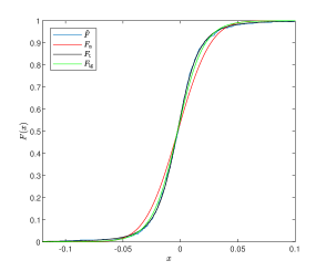
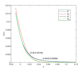
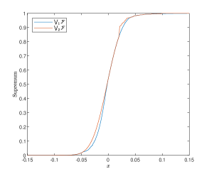
Figure 2: Left: cdf; Middle: Integrated survival function; Right: Suprema of $\mathcal{F}$

In the following, we compare the ${\rm MA}_{1}$ and ${\rm MA}_{2}$ robust risk values and the WR ones with the uncertainty set $\mathcal{F}$. The risk measures are RVaR or ES. In the case of ${\rm RVaR}_{\alpha,\beta}$, we set $\alpha=0.95$ and let $\beta$ vary in $[0.95,1]$. In the case of $\mathrm{ES}_{\alpha}$, $\alpha$ varies in $[0.9,0.99]$.

Figure 3 shows the value of RVaR_α,β of the cdfs in $\mathcal{F}$, and RVaR_α,β based on the MA and WR approaches, and Figure 4 presents the results of ES. From both figures we can see that the MA robust risk value is larger than the WR one. Moreover, from Figure 3, one can find that these two robust approaches have identical performance for $\beta\in[0.95,0.9685]$. This is because the quantile function of $F_{\rm n}$ dominates other elements in $\mathcal{F}$ on $[0.95,0.9685]$ which implies that ${\rm RVaR}_{0.95,\beta}^{{\rm MA}_{1}}(\mathcal{F})={\rm RVaR}_{0.95,\beta}^{\rm WR}(\mathcal{F})={\rm RVaR}_{0.95,\beta}(F_{\rm n})$ for $\beta\in[0.95,0.9685]$. From Figure 4, we find that $\mathrm{ES}_{\alpha}(F_{\rm n})$ and $\mathrm{ES}_{\alpha}(F_{\rm lg})$ are always smaller than $\mathrm{ES}_{\alpha}(\hat{F})$ and $\mathrm{ES}_{\alpha}(F_{\rm t})$ for $\alpha\in[0.9,0.99)$. The reason is that financial market loss data are heavy-tailed empirically (see e.g., McNeil et al. (2015)), and ES with high level $\alpha$ focuses on the tail loss. In addition, the curve of $\mathrm{ES}^{\rm MA}$ always lies above the curve of $\mathrm{ES}^{\rm WR}$, which implies that the MA approach is more conservative.

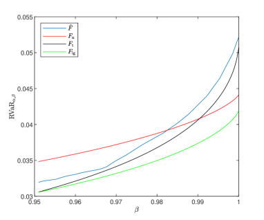
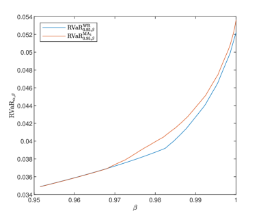
Figure 3: RVaR for individual models, via WR and via MA ($\alpha$=0.95)

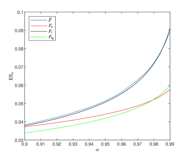
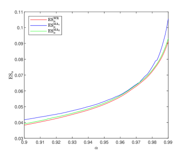
Figure 4: ES for individual models, via WR and via MA

8.2 MA approach in robust portfolio selection

In this section, we consider the application of the MA approach with $\preceq_{2}$ in the setting of portfolio selection in Section 6. The MA approach will be contrasted to the WR approach, and the standard sample average approximation (SAA) approach. We construct a portfolio from the 20 stocks mentioned in the beginning of this section, whose daily losses are denoted by $X_{1}$ (AAPL), $X_{2}$ (MSFT), …, $X_{20}$ (IBM). Mean, variance and correlation matrix of the return rate of the 20 stocks are given in Appendix G. The wealth invested in the asset $X_{i}$ is denoted by $w_{i}$ for $i\in[20]$. Thus, the total loss from the investment of these 20 stocks is $\mathbf{w}^{\top}\mathbf{X}$, where $\mathbf{w}=(w_{1},\dots,w_{20})$ and $\mathbf{X}=(X_{1},\dots,X_{20})$. The feasible region of $\mathbf{w}$ is the standard simplex $\Delta_{20}.$

We consider the setting in Section 6 where uncertainty is modeled by a multi-dimensional Wasserstein ball. For the choice of the risk measure $\rho$, we will work with ${\rm PD}_{k}$ defined in Section 6 to measure the portfolio risk. There are a few reasons for this choice. First, ${\rm PD}_{k}$ is $\preceq_{2}$-consistent (which also implies $\preceq_{1}$-consistency). Second, the WR and ${\rm MA}_{2}$ approaches are similar in the portfolio optimization problem under the Wasserstein or the mean-variance uncertainty if the risk measure is selected as ES or expectile, so we move away from these two choices. Third, the portfolio optimization problem of ${\rm PD}_{k}$ leads to a convenient formulation of SOCP under the Wasserstein or the mean-variance uncertainty as in Section 6.

As in many classic settings of portfolio selection, e.g., the classic framework of Markowitz (1952), we assume that the investor has a target level of expected annualized return rate and minimizes the risk. That is, with the constraint $\mathbb{E}[{\mathbf{w}}^{\top}{\mathbf{X}}]\leqslant-r_{0}/m$ where $r_{0}$ is the expected annualized return rate and $m=250$, the investor minimizes $\rho(F_{{\mathbf{w}}^{\top}{\mathbf{X}}})$.

We set the parameter $a=p=2$ in the Wasserstein uncertainty ball $\mathcal{F}_{a,p,\varepsilon}^{d}(F_{0})$, and use a multivariate t-benchmark distribution $F_{0}$ fitted to the data. The case of a normal benchmark distribution, which has a lighter tail, is reported in Appendix G. For the whole-period data, the fitted t-distribution has $\nu=3.994$ degrees of freedom. The choice of a t-distribution is by no means restrictive, and we will consider the case of normal distribution which has a lighter tail in Appendix. We apply the WR and the $\preceq_{2}$-MA approaches, and the corresponding portfolio optimization problems are converted to SOCPs which can be computed efficiently. By (28) and (29) in Section 6.2, the optimization problems via the WR and the MA approaches are, respectively,

$$\min_{{\mathbf{w}}\in\Delta_{20}}:~{}~{}\rho^{\rm WR}\left(\mathcal{F}_{\mathbf{w},2,2,\varepsilon}(F_{0})\right)={\mathbf{w}}^{\top}\bm{\mu}+{\rm PD}_{k}(F_{\nu})\sqrt{{\mathbf{w}}^{\top}\Sigma{\mathbf{w}}}+\zeta_{k}\varepsilon\sqrt{{\mathbf{w}}^{\top}{\mathbf{w}}}~{}~{}~{}~{}{\rm s.t.}~{}{\mathbf{w}}^{\top}\bm{\mu}\leqslant-r_{0}/m,$$ (37)

and

$$\min_{{\mathbf{w}}\in\Delta_{20}}:~{}~{}\rho^{{\rm MA}_{2}}\left(\mathcal{F}_{\mathbf{w},2,2,\varepsilon}(F_{0})\right)={\mathbf{w}}^{\top}{\bm{\mu}}+{\rm PD}_{k}(F_{\nu})\sqrt{{\mathbf{w}}^{\top}\Sigma{\mathbf{w}}}+\xi_{k}\varepsilon\sqrt{{\mathbf{w}}^{\top}{\mathbf{w}}}~{}~{}~{}~{}{\rm s.t.}~{}{\mathbf{w}}^{\top}\bm{\mu}\leqslant-r_{0}/m,$$ (38)

where $\zeta_{k}={k}/{\sqrt{2k-1}}$, $\xi_{k}=(\sqrt{\pi}\Gamma(k+1))/(2\Gamma(k+1/2))$, $F_{\nu}$ is the unit variance t-distribution with the tail parameter $\nu$, and $\bm{\mu}$ and $\Sigma$ are the mean and the covariance of the fitted $F_{0}$, i.e., the mean vector and the covariance of the whole-period data. The SAA approach optimizes the portfolio according to the empirical cdf of the asset losses. Figure 5 presents the optimized risk value of SAA approach and the optimized robust risk values under Wasserstein uncertainty with the WR and MA approaches for different values of $\varepsilon$, $r_{0}$ and $k$ using the whole-period data. In the left panel, the MA robust risk value is larger than the WR one, and both are generally larger than that of SSA. This is consistent with our intuition as MA is more conservative than WR, and SAA is not a conservative method. In the middle and the right panels we set $\varepsilon=0.01$ and let $k$ and $r$ vary. In practice, the parameter $\varepsilon$ should not be too small; one may tune $\varepsilon$ so that the empirical cdf remains in the Wasserstein ball.

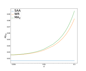
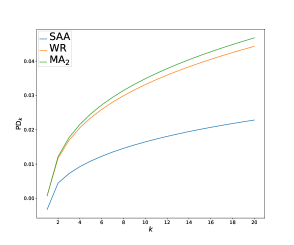
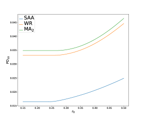
Figure 5: The optimized robust values of ${\rm PD}_{k}$ under Wasserstein uncertainty using the whole-period data. Left: $r_{0}=0.2$, $k=10$, $\varepsilon\in[0,0.1]$; Middle: $r_{0}=0.2$, $\varepsilon=0.01$, $k\in[1,20]$; Right: $k=10$, $\varepsilon=0.01$, $r_{0}\in[0.15,0.5]$

We choose slightly more than half of the period (350 trading days) for the initial training, and optimize the portfolio weights in each day with a rolling window. That is, on each trading day starting from day 351 (roughly June 2020), the preceding 350 trading days are used to fit the benchmark distribution, and compute the optimal portfolio weights. Note that the parameter $k$ reflects the degree of risk aversion of the decision maker, that is, a larger value of $k$ indicates a more risk-averse decision maker, and thus a larger corresponding risk measure. In this experiment, we choose $k=2$ and $20$, and the decision maker with $k=20$ is more risk-averse than the one with $k=2$. Figure 6 depicts the performance of SAA approach, the mean-variance model of Markowitz (1952) (minimizing the variance of $\mathbf{w}^{\top}{\mathbf{X}}$ subject to $\mathbb{E}[{\mathbf{w}}^{\top}{\mathbf{X}}]\leqslant-r_{0}/m$), and the MA and WR approaches under Wasserstein uncertainty over the remaining 300 trading days with $r_{0}=0.2$ and $\varepsilon=0.01$, and we set $k=2$ (left) or $k=20$ (right). Table 2 presents realized annualized return rates and Sharpe ratios of all methods. In all results, the MA and WR approaches, being robust methods, perform similarly. MA and WR generally outperform the SAA and the Markowitz model, especially after the first 150 trading days. Intuitively, this means that, during the period from Jan to Aug 2021, robust investment strategies likely outperform non-robust strategies. The similar performance of the MA and WR approaches under Wasserstein uncertainty is not a coincidence due to the similarity of problems (37) and (38) by noting that $\varepsilon$ is small.

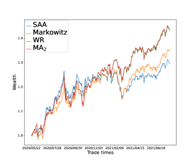
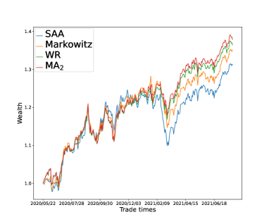
Figure 6: Wealth evolution for different portfolio strategies from May 2020 to Aug 2021 ($\varepsilon=0.01$, $r_{0}=0.2$). Left: $k=2$; Right: $k=20$

Table 2: Annualized return (AR), annualized volatility (AV) and Sharpe ratio (SR) for different strategies from May 2020 to Aug 2021; $r_{0}=0.2$ and the risk-free rate is $0.165\%$ (1-year US Treasury yield on May 22, 2020)

	AR ($\%$)		AV ($\%$)		SR ($\%$)
Approach	$k=2$	$k=20$	$k=2$	$k=20$	$k=2$	$k=20$
SAA	25.42	26.72	14.82	14.35	170.4	185.0
Markowitz	29.50	29.50	13.54	13.54	216.6	216.6
WR	32.75	30.79	14.25	13.30	228.7	230.3
${\rm MA}_{2}$	33.77	32.01	14.48	13.56	232.0	234.9

Table 3 presents the nominal transaction cost for different strategies by using the average weight change $\sum_{t=1}^{T}\|\mathbf{w}_{t+1}-\mathbf{w}_{t}\|_{1}/T$ where $\mathbf{w}_{t}$ is the weight used on day $t\in[T]$ by each strategy (see Olivares-Nadal and DeMiguel (2018)). The MA and WR approaches based on Wasserstein uncertainty have similar transaction costs, which are smaller than the other methods in most cases. A similar analysis using the mean-variance uncertainty is reported in Appendix G.

Table 3: Nominal transaction cost $\sum_{t=1}^{T}\|\mathbf{w}_{t+1}-\mathbf{w}_{t}\|_{1}/T$ with $\varepsilon=0.01$ and $T=299$

	$r_{0}=0.1$		$r_{0}=0.2$		$r_{0}=0.3$
Approach	$k=2$	$k=20$	$k=2$	$k=20$	$k=2$	$k=20$
SAA	0.0549	0.0071	0.0871	0.0121	0.0969	0.0833
Markowitz	0.0102	0.0102	0.0110	0.0110	0.0746	0.0746
WR	0.0127	0.0032	0.0127	0.0033	0.0271	0.0382
${\rm MA}_{2}$	0.0114	0.0035	0.0105	0.0035	0.0239	0.0348

9 Concluding remarks and discussions

The MA approach for robust risk evaluation is proposed. Below, we summarize some the advantages of the MA approach, which are illustrated and discussed through several technical results.

1. The MA approach is natural to interpret, and it is motivated by the need for a robust distributional model. The WR approach is also natural to interpret, but the focus is on the risk value instead of the risk model. Different from the WR approach, the MA approach is built on stochastic orders and lattice theory. The robust model produced by the MA approach can be readily applied to different risk evaluation procedures and decision problems (Section 3).

2. The MA robust risk value is straightforward to compute (Section 4.1). In some settings of uncertainty, the MA approach leads to explicit formulas for the robust model (Section 6). In particular, it can handle Wasserstein uncertainty in portfolio selection, based on a new dimension reduction result on Wasserstein balls (Theorem 5).

3. The MA approach admits reformulations in robust optimization similar to the WR approach, and it leads to a convex program when the loss function and the risk measure are convex (Section 5).

4. The MA approach gives rise to the useful property of cEMA which characterizes VaR and ES (Section 7). These results reveal a profound connection of the popular regulatory risk measures to robust risk evaluation methods, and highlight the special roles of VaR and ES among all risk measures, which is in itself a highly active research topic in risk management.

The MA approach requires a stochastic order to be specified. For an interpretation of prudent risk evaluation as in (3), the risk measure of interest should be consistent with this stochastic order. We recommend, in most applications, using $\preceq_{2}$ in an MA approach as the default option, for its nice interpretation in decision theory (strong risk aversion) and mathematical properties as developed in this paper.

We have focused on studying the MA and WR approaches together with risk measures throughout the paper. Both approaches can be easily applied to other objectives other than risk measures, such as expected utility functions, rank-dependent expected utilities, or other behaviour decision criteria. Some decision criteria may work better with notions of stochastic dominance other than FSD and SSD, and they may include considerations of model uncertainty by design; see e.g., Hansen and Sargent (2001), Maccheroni et al. (2006) and Cerreia-Vioglio et al. (2021).

Our theory is built on model spaces of univariate cdfs on $\mathbb{R}$ for the following reasons. First, classic risk measures, especially the ones used in regulatory practice such as VaR and ES, are defined on one-dimensional cdfs representing potential (portfolio) losses; second, commonly used stochastic orders, the key tool to build robust model aggregation in this paper, are usually defined on one-dimensional cdfs and they are naturally interpretable in this setting; third, many problems that are multivariate in natural often boil down to robust risk evaluation in one-dimension; see the settings in Sections 6.2, 6.3 and 8.2. If desired by specific applications, the theory of the MA approach can be readily extended to a multi-dimensional setting (see e.g., Embrechts and Puccetti (2006)) with the help from multivariate stochastic orders (e.g., Shaked and Shanthikumar (2007)) and set-valued risk measures (e.g., Hamel and Heyde (2010), Hamel et al. (2011) and Ararat et al. (1999)).

In addition to the multi-dimensional extension mentioned above, we mention a few promising directions of future study. First, one can consider the recently introduced notions of fractional stochastic dominance of Müller et al. (2017) and Huang et al. (2020), which generalize the first- and second-order stochastic dominance used in this paper. Second, instead of relying only on the set $\mathcal{F}$ of uncertainty, which treats each cdf as an element of equal importance ex ante, we can equip a prior probability measure $\mu$ on set $\mathcal{F}$, and this will open up many new challenges or conceptualizing and constructing robust models in a similar framework to our theory. Third, we can apply the MA approach to many other settings of uncertainty other than the ones studied in Section 6, and this will lead to convenient tools in various new applications and contexts.

We organize the appendices as follows. We first introduce some extra notation and terminology in Appendix A. In Appendix B, we formally introduce the lattice theory and prove a generalized version of Proposition 1 in Section 4. The proofs of the main results are presented in Appendices C (other results in Section 4), D (results in Section 5), E (results and omitted figures in Section 6) and F (results in Section 7). In Appendix G, we present the summary statistics of the return rates as well as the numerical results in portfolio selection under mean-variance uncertainty and Wasserstein uncertainty with a normal benchmark distribution, which complements the numerical studies in Section 8.

Appendix A Setting and notation

We will use the same notation as in the main paper. In addition, let $L^{p}$ be the space of random variables in $(\Omega,\mathcal{B},\mathbb{P})$ with finite $p$th moment, $p\in[0,\infty)$, and $L^{\infty}$ be the space of all bounded random variables. Accordingly, denote by $\mathcal{M}_{p}$, $p\in[0,\infty]$, the set of cdfs of all random variables in $L^{p}$, i.e., $\mathcal{M}_{p}$ is the set of all cdfs $F$ satisfying $\int_{\mathbb{R}}|x|^{p}\mathrm{d}F(x)<\infty$ for $p\in[0,\infty)$, and $\mathcal{M}_{\infty}$ is the set of all compactly supported cdfs. On $\mathcal{M}_{\infty}$, we can define $\mathrm{VaR}_{0}$, $\mathrm{VaR}_{1}$ and $\mathrm{ES}_{1}$ which are finite, by

$$\mathrm{VaR}_{0}(F)=\inf\{x\in\mathbb{R}:F(x)>0\}~{}\mbox{ and }~{}\mathrm{VaR}_{1}(F)=\inf\{x\in\mathbb{R}:F(x)\geqslant 1\},~{}~{}~{}F\in\mathcal{M}_{\infty},$$

and

$$\mathrm{ES}_{1}(F)={\rm VaR}_{1}(F),~{}~{}~{}F\in\mathcal{M}_{\infty}.$$

Denote by $\mathcal{M}_{\rm bb}$ the set of all cdfs $F$ with a support bounded from below, i.e., $F(x_{0})=0$ for some $x_{0}\in\mathbb{R}$. For two real objects (numbers or functions) $f$ and $g$, $f\vee g$ is their (point-wise) maximum, and $f\wedge g$ is their (point-wise) minimum.

For $p\in[0,\infty]$, the following are some properties of a risk measure $\rho:\mathcal{M}_{p}\to\mathbb{R}$ and its associated $\widetilde{\rho}:L^{p}\to\mathbb{R}$. Translation invariance: $\widetilde{\rho}(X+c)=\widetilde{\rho}(X)+c$ for any $c\in\mathbb{R}$ and $X\in L^{p}$. Positive homogeneity: $\widetilde{\rho}({\lambda X})=\lambda\widetilde{\rho}(X)$ for any $\lambda>0$ and $X\in L^{p}$. Convexity: $\widetilde{\rho}({\lambda X+(1-\lambda)Y})\leqslant\lambda\widetilde{\rho}(X)+(1-\lambda)\widetilde{\rho}(Y)$ for any $\lambda\in[0,1]$ and $X,Y\in L^{p}$. Lower semicontinuity: $\liminf_{n\to\infty}\widetilde{\rho}(X_{n})\geqslant\widetilde{\rho}(X)$ if $X_{n},X\in L^{p}$ for all $n$ and $X_{n}\stackrel{{\scriptstyle\rm d}}{{\to}}X$ as $n\to\infty$, where $\stackrel{{\scriptstyle\rm d}}{{\to}}$ denotes convergence in distribution. All the properties are defined for both $\rho$ and $\widetilde{\rho}$.

Appendix B Lattice theory and the proof of Proposition 1

In this appendix, we introduce the lattice structure of an ordered set which complements the main paper. For more details of the lattice theory, the reader is referred to Davey and Priestley (2002).

Definition EC.1.

Let $(\mathcal{M},\preceq)$ be an ordered set (i.e., $\preceq$ is a partial order on $\mathcal{M}$) and $\mathcal{F}\subseteq\mathcal{M}$.

• A set $\mathcal{F}$ is said to be bounded from above (below, resp.) in $(\mathcal{M},\preceq)$, if the set of upper (lower, resp.) bounds on $\mathcal{F}$, denoted by $U(\mathcal{F})$ ($L(\mathcal{F})$, resp.), is nonempty, where

  $$U(\mathcal{F})=\{G\in\mathcal{M}:F\preceq G,~{}{\forall}F\in\mathcal{F}\}~{}~{}{\rm and}~{}~{}L(\mathcal{F})=\{G\in\mathcal{M}:G\preceq F,~{}{\forall}F\in\mathcal{F}\}.$$ (EC.1)

• For $\mathcal{F}\subseteq\mathcal{M}$ which is bounded from above (below, resp.), if there exists $F_{0}\in U(\mathcal{F})$ ($L(\mathcal{F})$, resp.) such that $F_{0}\preceq$ ($\succeq$, resp.) $G$ for all $G\in U(\mathcal{F})$ ($L(\mathcal{F})$, resp.), then $F_{0}$ is called the supremum (infimum, resp.) of $\mathcal{F}$ and we write $\bigvee\mathcal{F}=F_{0}$ ($\bigwedge\mathcal{F}=F_{0}$, resp.).

• If for all $F,G\in\mathcal{M}$, $\bigvee\{F,G\}$ and $\bigwedge\{F,G\}$ exist, then $(\mathcal{M},\preceq)$ is called a lattice. If $\bigvee\mathcal{F}$ exists for all $\mathcal{F}\subseteq\mathcal{M}$ that are bounded from above and $\bigwedge\mathcal{F}$ exists for all $\mathcal{F}\subseteq\mathcal{M}$ that are bounded from below, then $(\mathcal{M},\preceq)$ is called a complete lattice.

Remark EC.1.

In case $(\mathcal{M},\preceq)$ is a lattice which is not complete, $\bigvee\mathcal{F}$ may not exist even if $\mathcal{F}$ is bounded from above. In this case, the definition of the MA robust risk value needs to be modified. We can alternatively define $\rho^{\rm MA}(\mathcal{F})=\inf_{G\in U(\mathcal{F})}\rho(G)$ where $U(\mathcal{F})$ is defined by (EC.1), and this definition is equivalent to (2) if $(\mathcal{M},\preceq)$ is a complete lattice and $\rho$ is $\preceq$-consistent. For any partial order $\preceq$, the supreme and infimum are both unique whenever it exists.

For stochastic dominances $\preceq_{1}$ and $\preceq_{2}$, there are several equivalent definitions that are useful throughout the paper; see e.g., Bäuerle and Müller (2006). In case of $\preceq_{1}$, the following statements are equivalent: (i) $F\preceq_{1}G$; (ii) $F(x)\geqslant G(x)$ for all $x\in\mathbb{R}$; (iii) $F^{-1}(\alpha)\leqslant G^{-1}(\alpha)$ for all $\alpha\in(0,1)$. In case of $\preceq_{2}$, the following statements are equivalent: (i) $F\preceq_{2}G$; (ii) $\pi_{F}(x)\leqslant\pi_{G}(x)$ for all $x\in\mathbb{R}$ where $\pi_{F}$ is the integrated survival function defined by (10); (iii) $E_{F}(\alpha)\leqslant E_{G}(\alpha)$ for all $\alpha\in(0,1)$ where $E_{F}$ is the integrated quantile function defined by

$$E_{F}(\alpha)=(1-\alpha)\mathrm{ES}_{\alpha}(F)=\int_{\alpha}^{1}F^{-1}(s){\mathrm{d}}s,~{}~{}\alpha\in[0,1].$$ (EC.2)

The complete lattice structure of $(\mathcal{M}_{0},\preceq_{1})$ and $(\mathcal{M}_{+},\preceq_{2})$ and the formulas for the suprema are known in the literature; see Kertz and Rösler (2000). Here $\mathcal{M}_{+}=\{F\in\mathcal{M}_{0}:\int_{0}^{\infty}x{\mathrm{d}}F(x)<\infty\}$. The following proposition which is a generalized result of Proposition 1 considers general space $\mathcal{M}_{p}$, $p\in[0,\infty]$ with partial order $\preceq_{1}$ and $\preceq_{2}$. Specifically, in Proposition EC.1 below, (a) generalizes Proposition 1 (a) to the domain $\mathcal{M}_{p}$, $p\in[0,\infty]$, and similarly, (b) and (c) generalize Proposition 1 (b).

Proposition EC.1.

• For each $p\in[0,\infty]$, the ordered set $(\mathcal{M}_{p},\preceq_{1})$ is a complete lattice with the supremum $\bigvee_{1}\mathcal{F}=\inf_{F\in\mathcal{F}}F$ for $\mathcal{F}\subseteq\mathcal{M}_{p}$ which is bounded from above. The left quantile function of $\bigvee_{1}\mathcal{F}$ is $\sup_{F\in\mathcal{F}}F^{-1}$.

• The ordered set $(\mathcal{M}_{1},\preceq_{2})$ is a complete lattice, and for $\mathcal{F}$ which is bounded from above,

  $$\pi_{\bigvee_{2}\mathcal{F}}=\sup_{F\in\mathcal{F}}\pi_{F},~{}~{}~{}~{}~{}\bigvee_{2}\mathcal{F}=1+\left(\sup_{F\in\mathcal{F}}\pi_{F}\right)^{\prime}_{+}.$$

• For each $p\in(1,\infty]$, the ordered set $(\mathcal{M}_{p},\preceq_{2})$ is a lattice and not a complete lattice. The supremum is given by $\bigvee_{2}\{F,G\}=1+(\pi_{F}\vee\pi_{G})_{+}^{\prime}$ for $F,G\in\mathcal{M}_{p}$.

Proof.

We first give one fact: For $p\in[0,\infty]$ and an increasing and right-continuous function $H:\mathbb{R}\to[0,1]$, if $F,G\in\mathcal{M}_{p}$ and $F\leqslant H\leqslant G$, then $H\in\mathcal{M}_{p}$. It suffices to verify that

• $0\leqslant\lim_{x\to-\infty}H(x)\leqslant\lim_{x\to-\infty}G(x)=0$ and $1\geqslant\lim_{x\to\infty}H(x)\geqslant\lim_{x\to-\infty}F(x)=1$, which imply that $H$ is a cdf on $\mathbb{R}$, that is, $H\in\mathcal{M}_{0}$.

• If $p\in(0,\infty)$, then we have $F\succeq_{1}H\succeq_{1}G$ and thus $\int_{0}^{\infty}x^{p}\mathrm{d}H(x)\leqslant\int_{0}^{\infty}x^{p}\mathrm{d}F(x)<\infty$ and $\int_{-\infty}^{0}(-x)^{p}\mathrm{d}H(x)\leqslant\int_{-\infty}^{0}(-x)^{p}\mathrm{d}G(x)<\infty$. It follows that $\int_{\mathbb{R}}|x|^{p}\mathrm{d}H(x)<\infty,$ that is, $H\in\mathcal{M}_{p}$.

• If $F,G\in\mathcal{M}_{\infty}$, then there exists $x$, $y\in\mathbb{R}$ such that $G(x)=0$ and $F(y)=1$. Then we have $H(x)=0$ and $H(y)=1$, that is, $H\in\mathcal{M}_{\infty}$.

(a) For $p\in[0,\infty]$, let $\mathcal{F}\subseteq\mathcal{M}_{p}$. Suppose that $\mathcal{F}$ is bounded from above. Define $H=\inf_{F\in\mathcal{F}}F$ which is increasing and right-continuous. Then there exists $G\in\mathcal{M}_{p}$ such that $F\geqslant H\geqslant G$ for any $F\in\mathcal{F}$. By the above fact, we have $H\in\mathcal{M}_{p}$. If $\mathcal{F}$ is bounded from below, define $H(x)=\lim_{y\downarrow x}H_{1}(y)$ where $H_{1}=\sup_{F\in\mathcal{F}}F$. Then $H$ is increasing and right-continuous and there exists $G\in\mathcal{M}_{p}$ such that $G\geqslant H\geqslant F$ for any $F\in\mathcal{F}$. By the above fact, we have $H\in\mathcal{M}_{p}$. Therefore, we have that $(\mathcal{M}_{p},\preceq_{1})$ is a complete lattice for $p\in[0,\infty]$. The statement on the left quantile of $\bigvee_{1}\mathcal{F}$ follows from $(\inf_{F\in\mathcal{F}}F)^{-1}=\sup_{F\in\mathcal{F}}F^{-1}$. Hence, we complete the proof of (a).

(b) The proof is similar to that of Theorem 3.4 of Kertz and Rösler (2000) which shows that $(\mathcal{M}_{+},\preceq_{2})$ is a complete lattice. We give a proof for completeness. Let $\mathcal{F}\subseteq\mathcal{M}_{1}$ be bounded from above. There exists $G\in\mathcal{M}_{1}$ such that $F\preceq_{2}G$ for all $F\in\mathcal{F}$, that is, $\sup_{F\in\mathcal{F}}\pi_{F}(x)\leqslant\pi_{G}(x)$ for $x\in\mathbb{R}$. One can check that

• $\pi_{0}(x):=\sup_{F\in\mathcal{F}}\pi_{F}(x)$ is decreasing convex as each $\pi_{F}(x)$ is decreasing convex. This implies $1+(\pi_{0})_{+}^{\prime}(x)$ is right-continuous and increasing.

• $\lim_{x\to\infty}\pi_{0}(x)\leqslant\lim_{x\to\infty}\pi_{G}(x)=0$ which implies $\lim_{x\to\infty}(\pi_{0})_{+}^{\prime}(x)=0$, that is, $\lim_{x\to\infty}(1+(\pi_{0})_{+}^{\prime}(x))=1$.

• Since $x+\pi_{F}(x)$ is increasing in $x$ for all $F\in\mathcal{F}$, we have $x+\pi_{0}(x)$ is increasing in $x$ and thus $\lim_{x\to-\infty}x+\pi_{0}(x)$ exists (may take $-\infty$). Let $F^{*}\in\mathcal{F}$, and we have $x+\pi_{0}(x)\geqslant x+\pi_{F^{*}}(x)$ for all $x\in\mathbb{R}$. Noting that $\lim_{\color[rgb]{0,0,0}x\to-\infty}x+\pi_{F^{*}}(x)=\mathfrak{m}({F^{*}})\in\mathbb{R}$, we have $\lim_{x\to-\infty}x+\pi_{0}(x)\in\mathbb{R}$, which implies $\lim_{x\to-\infty}1+(\pi_{0})_{+}^{\prime}(x)=0$.

Combining the above three observations, we have $H=1+(\sup_{F\in\mathcal{F}}\pi_{F})_{+}^{\prime}\in\mathcal{M}_{1}$. By definition of supremum, it is standard to check that $\bigvee_{2}\mathcal{F}=H$.

Let $\mathcal{F}\subseteq\mathcal{M}_{1}$ be bounded from below. There exists $G\in\mathcal{M}_{1}$ such that $G\preceq_{2}F$ for all $F\in\mathcal{F}$, that is, $E_{G}(\alpha)\leqslant\inf_{F\in\mathcal{F}}E_{F}(\alpha)$ for $\alpha\in[0,1]$. Similar to the proof of Steps 1-3 for $\mathcal{F}$ that is bounded from above, one can show that $\inf_{F\in\mathcal{F}}E_{F}$ is an integrated quantile function of some cdf in $\mathcal{M}_{1}$, say $H$. By definition of infimum, we have $H=\bigwedge_{2}\mathcal{F}$. It follows from the relation between a cdf and its integrated quantile function that $H^{-1}=-(\inf_{F\in\mathcal{F}}E_{F})_{-}^{\prime}$. This completes the proof of (b).

(c) For $F,G\in\mathcal{M}_{p}$, define $F_{1}=\bigvee_{2}\{F,G\}$ and $F_{2}=\bigwedge_{2}\{F,G\}.$ It follows from (b) that $F_{1}=1+(\pi_{F}\vee\pi_{G})_{+}^{\prime}$ which implies $\min\{F,G\}\leqslant F_{1}\leqslant\max\{F,G\}$, and $F_{2}^{-1}=-(E_{F}\wedge E_{G})_{-}^{\prime}$ which implies $\min\{F^{-1},G^{-1}\}\leqslant F_{2}^{-1}\leqslant\max\{F^{-1},G^{-1}\}$, and hence, $\min\{F,G\}\leqslant F_{2}\leqslant\max\{F,G\}$. By the fact in the beginning of the proof, we have $F_{1},F_{2}\in\mathcal{M}_{p}$, and thus $(\mathcal{M}_{p},\preceq_{2})$ is a lattice for $p\in(1,\infty]$.

Below, we give a counterexample to illustrate that $(\mathcal{M}_{p},\preceq_{2})$ is not complete lattice for $p\in(1,\infty]$. For $p\in(1,\infty)$, define $F(x)=(-x)^{-p}$ for $x\leqslant-1$. We have $F\not\in\mathcal{M}_{p}$ and for $y<-1,$ let $F_{y}$ be a cdf with integrated survival function

$$\pi_{F_{y}}(x)=\max\left\{\left(-x-\frac{p}{p-1}\right)_{+},\,\,\pi_{F}^{\prime}(y)(x-y)+\pi_{F}(y)\right\}.$$

It is clear that $F_{y}\in\mathcal{M}_{\infty}$ for all $y<-1$ and the set $\{F_{y}\}_{y<-1}$ is bounded from above as $F_{y}\preceq_{2}\delta_{-1}$ for $y<-1$. Noting that $\sup_{y<-1}\pi_{F_{y}}=\pi_{F}$ and $F\not\in\mathcal{M}_{p}$, we have that $(\mathcal{M}_{p}\preceq_{2})$ is not a complete lattice. ∎

Appendix C Proofs for other results in Sections 4

Proof of Proposition 2.  For a fixed $x\in\mathbb{R}$, both $F\mapsto F(x)$ and $F\mapsto\pi_{F}(x)$ are linear in $F$. Hence, for $F\in{\rm conv}\mathcal{F}$ with $F=\sum_{i=1}^{n}\lambda_{i}F_{i}$ where $(\lambda_{1},\dots,\lambda_{n})\in\Delta_{n}$ and $F_{i}\in\mathcal{F}$ for $i\in[n]$, there exist $G_{1},G_{2}\in\{F_{1},\dots,F_{n}\}\subseteq\mathcal{F}$ such that $G_{1}(x)\leqslant F(x)$ and $\pi_{G_{2}}(x)\geqslant\pi_{F}(x)$. The results follow immediately from Proposition 1. ∎

Proof of Theorem 1.  (a) Since $\mathfrak{m}(F)=\lim_{x\to-\infty}\left\{x+\pi_{F}(x)\right\}$ for each $F\in\mathcal{M}_{1}$, we have

$$\mathfrak{m}^{{\rm MA}_{2}}(\mathcal{F}) =\mathfrak{m}\left(\bigvee_{2}\mathcal{F}\right){\color[rgb]{0,0,0}=\lim_{x\to-\infty}\left\{x+\pi_{\bigvee_{2}\mathcal{F}}(x)\right\}}=\lim_{x\to-\infty}\left\{x+\sup_{F\in\mathcal{F}}\pi_{F}(x)\right\}$$

$$=\lim_{x\to-\infty}\sup_{F\in\mathcal{F}}\left\{\mathfrak{m}(F)+\int_{\mathbb{R}}(x-y)_{+}\mathrm{d}F(y)\right\}\leqslant\sup_{F\in\mathcal{F}}\mathfrak{m}(F)+\lim_{x\to-\infty}\sup_{F\in\mathcal{F}}\int_{\mathbb{R}}(x-y)_{+}\mathrm{d}F(y)$$

$$=\sup_{F\in\mathcal{F}}\mathfrak{m}(F)=\mathfrak{m}^{\rm WR}(\mathcal{F}),$$

where the third equality comes from (ii) of Proposition 1, and the forth equality follows from $x+\pi_{F}(x)=x+\mathbb{E}^{F}[(X-x)_{+}]=\mathfrak{m}(F)+\mathbb{E}^{F}[(x-X)_{+}]$. The converse direction $\mathfrak{m}^{{\rm MA}_{2}}(\mathcal{F})\geqslant\mathfrak{m}^{\rm WR}(\mathcal{F})$ is trivial. Hence, we complete the proof of (a).

(b) Suppose that $\mathcal{F}\subseteq\mathcal{M}_{1}$ is a convex set which is $\preceq_{2}$-bounded. Denote by $\Pi_{\mathcal{G}}=\sup_{F\in\mathcal{G}}\pi_{F}$ for any set $\mathcal{G}\subseteq\mathcal{M}_{1}$. If $\mathcal{G}$ is a convex polytope, then by Theorem 1 of Zhu and Fukushima (2009), we have

$$\mathrm{ES}_{\alpha}^{\rm WR}(\mathcal{G}) =\mathrm{ES}_{\alpha}^{{\rm MA}_{2}}(\mathcal{G}).$$ (EC.3)

Let $c=\mathrm{ES}_{\alpha}^{{\rm MA}_{2}}(\mathcal{F})$. Using (14), we get

$$x+\frac{1}{1-\alpha}\Pi_{\mathcal{F}}(x)\geqslant c\mbox{~{}~{}for all $x\in\mathbb{R}$.}$$ (EC.4)

Take an arbitrary $G\in\mathcal{F}$. Since $(\pi_{G})_{+}^{\prime}(x)\to-1$ as $x\to-\infty$, we have $(1-\alpha)x+\pi_{G}(x)\to\infty$ as $x\to-\infty$. There exists $x_{0}<c$ such that

$$x+\frac{1}{1-\alpha}\pi_{G}(x)\geqslant c\mbox{~{}~{}for all $x<x_{0}$.}$$ (EC.5)

Fix $\varepsilon>0$. Let $\mathcal{G}\subseteq\mathcal{F}$ be a convex polytope such that

$$\Pi_{\mathcal{G}}(x)\geqslant\Pi_{\mathcal{F}}(x)-\varepsilon\mbox{~{}~{}for all $x\in[x_{0},c]$}.$$ (EC.6)

We illustrate why such $\mathcal{G}$ exists. Let $\mathbb{Q}$ be a set of all rational numbers on $\mathbb{R}$, and we represent it as $\mathbb{Q}=\{q_{i}\}_{i\in\mathbb{N}}$. Suppose that $\{F_{i,j}\}_{j\in\mathbb{N}}\subseteq\mathcal{F}$ satisfies $\lim_{j\to\infty}\pi_{F_{i,j}}(q_{i})=\Pi_{\mathcal{F}}(q_{i})$ for $i\in\mathbb{N}$. Define $\mathcal{G}_{i}=\{F_{1,i},F_{2,i},\dots,F_{i,i}\}$ for $i\in\mathbb{N}$. It holds that $\Pi_{\mathcal{G}_{i}}(x)\to\Pi_{\mathcal{F}}(x)$ on $\mathbb{Q}$. By Theorem 10.8 of Rockafellar (1970), we have $\{\Pi_{\mathcal{G}_{i}}\}_{i\in\mathbb{N}}$ uniformly converges to $\Pi_{\mathcal{F}}$ on $[x_{0},c]$. This implies that such $\mathcal{G}$ in (EC.6) exists. Let $\mathcal{G}_{0}=\mathrm{conv}(\mathcal{G}\cup\{G\})\subseteq\mathcal{F}$, which is again a convex polytope. Using (EC.3), (EC.4), (EC.5) and (EC.6), we obtain

$$\mathrm{ES}_{\alpha}^{\rm WR}(\mathcal{G}_{0}) =\mathrm{ES}_{\alpha}^{{\rm MA}_{2}}(\mathcal{G}_{0})=\min_{x\in\mathbb{R}}\left\{x+\frac{\Pi_{\mathcal{G}_{0}}(x)}{1-\alpha}\right\}$$

$$=\min\left\{\inf_{x<x_{0}}\left\{x+\frac{\Pi_{\mathcal{G}_{0}}(x)}{1-\alpha}\right\},\min_{x\in[x_{0},c]}\left\{x+\frac{\Pi_{\mathcal{G}_{0}}(x)}{1-\alpha}\right\},\inf_{x>c}\left\{x+\frac{\Pi_{\mathcal{G}_{0}}(x)}{1-\alpha}\right\}\right\}$$

$$\geqslant\min\left\{\inf_{x<x_{0}}\left\{x+\frac{\pi_{G}(x)}{1-\alpha}\right\},\min_{x\in[x_{0},c]}\left\{x+\frac{\Pi_{\mathcal{G}}(x)}{1-\alpha}\right\},c\right\}$$

$$\geqslant\min\left\{\min_{x\in[x_{0},c]}\left\{x+\frac{\Pi_{\mathcal{F}}(x)}{1-\alpha}-\frac{\varepsilon}{1-\alpha}\right\},c\right\}$$

$$\geqslant\min\left\{\min_{x\in\mathbb{R}}\left\{x+\frac{\Pi_{\mathcal{F}}(x)}{1-\alpha}\right\},c\right\}-\frac{\varepsilon}{1-\alpha}=c-\frac{\varepsilon}{1-\alpha}.$$

Note that $\mathrm{ES}_{\alpha}^{\rm WR}(\mathcal{F})\geqslant\mathrm{ES}_{\alpha}^{\rm WR}(\mathcal{G}_{0})\geqslant c-\varepsilon/(1-\alpha)$ because $\mathcal{G}_{0}\subseteq\mathcal{F}$. Since $\varepsilon$ is arbitrary, we get $\mathrm{ES}_{\alpha}^{\rm WR}(\mathcal{F})\geqslant c=\mathrm{ES}_{\alpha}^{{\rm MA}_{2}}(\mathcal{F}).$ Together with $\mathrm{ES}_{\alpha}^{\rm WR}(\mathcal{F})\leqslant\mathrm{ES}_{\alpha}^{{\rm MA}_{2}}(\mathcal{F})$, we obtain the desired equality $\mathrm{ES}_{\alpha}^{\rm WR}(\mathcal{F})=\mathrm{ES}_{\alpha}^{{\rm MA}_{2}}(\mathcal{F})$.

(c) It follows directly from Proposition 1.∎

Proof of Theorem 2.  (a) We first consider the convexity of $\widetilde{\rho}^{\rm WR}$. Suppose that $\widetilde{\rho}$ is convex. Note that $\widetilde{\rho}^{\rm WR}$ is the supremum of a family of functionals $\widetilde{\rho}^{Q}$, $Q\in\mathcal{Q}$. It suffices to verify that $\widetilde{\rho}^{Q}$ is convex on $L$ for all $Q\in\mathcal{Q}$. Let $Q\in\mathcal{Q}$ and $X_{1},X_{2}\in L$. By a version of Skorhod’s Theorem (see, e.g., Theorem 3.1 of Berti et al. (2007)), we can construct $X_{1}^{\prime},X_{2}^{\prime}$ such that $\mathbb{P}(X_{1}^{\prime}\leqslant x_{1},X_{2}^{\prime}\leqslant x_{2})=Q(X_{1}\leqslant x_{1},X_{2}\leqslant x_{2})$ for all $x_{1},x_{2}\in\mathbb{R}$, i.e., the joint cdf of $(X_{1},X_{2})$ under $Q$ is same as the joint cdf of $(X_{1}^{\prime},X_{2}^{\prime})$ under $\mathbb{P}$. Hence, we have

$$\widetilde{\rho}^{Q}(\lambda X_{1}+(1-\lambda)X_{2})=\widetilde{\rho}(\lambda X_{1}^{\prime}+(1-\lambda)X_{2}^{\prime})\leqslant\lambda\widetilde{\rho}({X_{1}^{\prime}})+(1-\lambda)\widetilde{\rho}({X_{2}^{\prime}})=\lambda\widetilde{\rho}^{Q}(X_{1})+(1-\lambda)\widetilde{\rho}^{Q}(X_{2}),$$

where the inequality follows from the convexity of $\rho$. This yields the convexity of $\widetilde{\rho}^{\rm WR}$.

To see the convexity of $\widetilde{\rho}^{{\rm MA}_{2}}$, by Theorem 2.2 of Kaina and Rüschendorf (2009), $\widetilde{\rho}:L^{1}\to\mathbb{R}$ is continuous with respect to the $L^{1}$-norm because $\widetilde{\rho}(X)\in\mathbb{R}$ for all $X\in L^{1}$. It then follows from Theorem 5.1 of Cerreia-Vioglio et al. (2011) that $\rho$ is $\preceq_{2}$-consistent. Define

$$\mathcal{G}=\left\{g:(0,1)\to\mathbb{R}|(1-\alpha)g(\alpha)~{}{\rm is~{}concave~{}for~{}}\alpha\in(0,1),~{}\lim_{\alpha\to 1}(1-\alpha)g(\alpha)=0\right\}.$$

One can check that $\mathcal{G}$ is a convex set. Define $g_{F}(\alpha)=\mathrm{ES}_{\alpha}(F)$ for $\alpha\in(0,1)$ and $F\in\mathcal{M}_{1}$, and $\mathcal{G}^{\prime}:=\{g_{F}:(0,1)\to\mathbb{R}|~{}F\in\mathcal{M}_{1}\}$. Below we verify that $\mathcal{G}=\mathcal{G}^{\prime}$. It is easy to see that $g_{F}\in\mathcal{G}$ for all $F\in\mathcal{M}_{1}$, and this yields $\mathcal{G}^{\prime}\subseteq\mathcal{G}$. On the other hand, for any $g\in\mathcal{G}$, define $h(\alpha)=(1-\alpha)g(\alpha)$ for $\alpha\in(0,1)$. It holds that $-h_{-}^{\prime}:(0,1)\to\mathbb{R}$ is left-continuous and increasing, where $h_{-}^{\prime}$ is the left derivative of $h$. This implies that it is a quantile function of a cdf $F$, i.e., $F^{-1}=-h_{-}^{\prime}$. Since $h$ is real-valued, we have $F\in\mathcal{M}_{1}$. Further, we have

$$g_{F}(\alpha)=\frac{1}{1-\alpha}\int_{\alpha}^{1}F^{-1}(s)\mathrm{d}s=\frac{1}{1-\alpha}\int_{\alpha}^{1}-h^{\prime}_{-}(s)\mathrm{d}s=\frac{1}{1-\alpha}h(\alpha)=g(\alpha),~{}~{}\alpha\in(0,1).$$

This implies $\mathcal{G}\subseteq\mathcal{G}^{\prime}$. Hence, we have concluded that $\mathcal{G}=\mathcal{G}^{\prime}$. Thus, there is a bijection relation between $\mathcal{G}$ and $\mathcal{G}^{\prime}$, based on which, we can define $\widehat{\rho}:\mathcal{G}\to\mathbb{R}$ as $\widehat{\rho}(g_{F})=\rho(F)$. Note that $F\preceq_{2}G$ if and only if $g_{F}(\alpha)\leqslant g_{G}(\alpha)$ for all $\alpha\in(0,1)$. Since $\rho$ is $\preceq_{2}$-consistent, we have

$$\widetilde{\rho}^{{\rm MA}_{2}}(X)=\rho\left(\bigvee_{2}{\mathcal{F}_{X|\mathcal{Q}}}\right) =\inf\left\{\rho(F):F\in\mathcal{M}_{1},~{}\sup_{Q\in\mathcal{Q}}\widetilde{\mathrm{ES}}_{\alpha}^{Q}(X)\leqslant g_{F}(\alpha),~{}~{}\forall\alpha\in(0,1)\right\}$$

$$=\inf\left\{\widehat{\rho}(g):g\in\mathcal{G},~{}\sup_{Q\in\mathcal{Q}}\widetilde{\mathrm{ES}}_{\alpha}^{Q}(X)\leqslant g(\alpha),~{}~{}\forall\alpha\in(0,1)\right\}$$

$$=\inf_{g\in\mathcal{G}}\left\{\widehat{\rho}(g)+\Theta(X,g)\right\},$$

where $\Theta(X,g)=0$ if $\sup_{Q\in\mathcal{Q}}\widetilde{\mathrm{ES}}_{\alpha}^{Q}(X)\leqslant g(\alpha)$ for all $\alpha\in(0,1)$, and $\Theta(X,g)=\infty$ otherwise. Therefore, it suffices to show that $\widehat{\rho}(g)+\Theta(X,g)$ is convex in $(X,g)\in L\times\mathcal{G}$. For any $g_{1},g_{2}\in\mathcal{G}$, there are two cdfs $F_{1},F_{2}\in\mathcal{M}_{1}$ such that $g_{1}=g_{F_{1}}$ and $g_{2}=g_{F_{2}}$. Let $U$ be a uniform random variable on $[0,1]$ under $\mathbb{P}$ (see e.g., Lemma A.27 of Föllmer and Schied (2016) for the existence). Define $X_{1}=F_{1}^{-1}(U)$ and $X_{2}=F_{2}^{-1}(U)$. It holds that $F_{X_{1}}=F_{1}$, $F_{X_{2}}=F_{2}$, and $X_{1},X_{2}$ are comonotonic. Note that $\mathrm{ES}$ is positively homogeneous and comonotonic additive. We have $\lambda g_{1}+(1-\lambda)g_{2}=g_{F_{\lambda X_{1}+(1-\lambda)X_{2}}}$ for all $\lambda\in[0,1]$. Hence, it holds that

$$\widehat{\rho}(\lambda g_{1}+(1-\lambda)g_{2})=\widetilde{\rho}({\lambda X_{1}+(1-\lambda)X_{2}})\leqslant\lambda\widetilde{\rho}({X_{1}})+(1-\lambda)\widetilde{\rho}({X_{2}})=\lambda\widehat{\rho}(g_{1})+(1-\lambda)\widehat{\rho}(g_{2}),$$

where we have used the convexity of $\rho$ in the inequality. This means that $\widehat{\rho}$ is convex on $\mathcal{G}$. It remains to verify that $\Theta(X,g)$ is convex on $L\times\mathcal{G}$. To see this, note that $\Theta\in\{0,\infty\}$. For $X_{1},X_{2}\in L$ and $g_{1},g_{2}\in\mathcal{G}$, it suffices to show that for any $\lambda\in[0,1]$, $\Theta(\lambda X_{1}+(1-\lambda)X_{2},\lambda g_{1}+(1-\lambda)g_{2})=\infty$ implies $\Theta(X_{i},g_{i})=\infty$ for either $i=1$ or $2$. Suppose now $\Theta(\lambda X_{1}+(1-\lambda)X_{2},\lambda g_{1}+(1-\lambda)g_{2})=\infty$. Then, the following holds for some $\alpha\in(0,1)$,

$$\lambda g_{1}+(1-\lambda)g_{2} <\sup_{Q\in\mathcal{Q}}\widetilde{\mathrm{ES}}_{\alpha}^{Q}(\lambda X_{1}+(1-\lambda)X_{2})$$

$$\leqslant\sup_{Q\in\mathcal{Q}}\left\{\lambda\widetilde{\mathrm{ES}}_{\alpha}^{Q}(X_{1})+(1-\lambda)\widetilde{\mathrm{ES}}_{\alpha}^{Q}(X_{2})\right\}\leqslant\lambda\sup_{Q\in\mathcal{Q}}\widetilde{\mathrm{ES}}_{\alpha}^{Q}(X_{1})+(1-\lambda)\sup_{Q\in\mathcal{Q}}\widetilde{\mathrm{ES}}_{\alpha}^{Q}(X_{2}).$$

This concludes that $g_{i}(\alpha)<\sup_{Q\in\mathcal{Q}}\widetilde{\mathrm{ES}}_{\alpha}^{Q}(X_{i})$ for either $i=1$ or $2$, which in turn implies $\Theta(X_{i},g_{i})=\infty$ for either $i=1$ or $2$. Hence, we have that $\widetilde{\rho}^{{\rm MA}_{2}}$ is convex.

(b) Define $f_{F}(\alpha)=\mathrm{VaR}_{\alpha}(F)$ for $\alpha\in(0,1)$ and $F\in\mathcal{M}_{1}$. Let $\mathcal{M}_{1}^{-1}=\{f_{F}:(0,1)\to\mathbb{R}|F\in\mathcal{M}_{1}\}$. Define $\widehat{\rho}:\mathcal{M}_{1}^{-1}\to\mathbb{R}$ as the risk measure satisfying $\widehat{\rho}(f_{F})=\rho(F)$. Noting that $\widetilde{\rho}$ satisfies comonotonic additivity, we have $\widehat{\rho}(f_{1}+f_{2})=\widehat{\rho}(f_{1})+\widehat{\rho}(f_{2})$ for all $f_{1},f_{2}\in\mathcal{M}_{1}^{-1}$. Suppose now $X_{1},X_{2}\in L$ are two comonotonic random variables. By Proposition 4.6 of Wang and Ziegel (2021) who prove that the mapping $X\mapsto\sup_{Q\in\mathcal{Q}}\widetilde{\mathrm{VaR}}_{\alpha}^{Q}(X)$ satisfies comonotonic additivity for all $\alpha\in(0,1)$, we have

$$\sup_{Q\in\mathcal{Q}}f_{F_{X_{1}+X_{2}}^{Q}}(\alpha) =\sup_{Q\in\mathcal{Q}}\widetilde{\mathrm{VaR}}_{\alpha}^{Q}(X_{1}+X_{2})$$

$$=\sup_{Q\in\mathcal{Q}}\widetilde{\mathrm{VaR}}_{\alpha}^{Q}(X_{1})+\sup_{Q\in\mathcal{Q}}\widetilde{\mathrm{VaR}}_{\alpha}^{Q}(X_{2})=\sup_{Q\in\mathcal{Q}}f_{F_{X_{1}}^{Q}}(\alpha)+\sup_{Q\in\mathcal{Q}}f_{F_{X_{2}}^{Q}}(\alpha),~{}~{}\forall\alpha\in(0,1).$$

Hence,

$$\widetilde{\rho}^{{\rm MA}_{1}}(X_{1}+X_{2}) =\rho\left(\bigvee_{1}{\mathcal{F}_{X_{1}+X_{2}|\mathcal{Q}}}\right)=\widehat{\rho}\left(\sup_{Q\in\mathcal{Q}}f_{F_{X_{1}+X_{2}}^{Q}}\right)$$

$$=\widehat{\rho}\left(\sup_{Q\in\mathcal{Q}}f_{F_{X_{1}}^{Q}}+\sup_{Q\in\mathcal{Q}}f_{F_{X_{2}}^{Q}}\right)=\widehat{\rho}\left(\sup_{Q\in\mathcal{Q}}f_{F_{X_{1}}^{Q}}\right)+\widehat{\rho}\left(\sup_{Q\in\mathcal{Q}}f_{F_{X_{2}}^{Q}}\right)$$

$$=\widetilde{\rho}^{{\rm MA}_{1}}(X_{1})+\widetilde{\rho}^{{\rm MA}_{1}}(X_{2}).$$

This yields the comonotonic additivity of $\widetilde{\rho}^{{\rm MA}_{1}}$.

(c) We only consider the case of translation invariance as the case of positive homogeneity is similar. Suppose that $\widetilde{\rho}$ satisfies translation invariance. We have $\rho(G)=\rho(F)+c$ whenever $F,G\in\mathcal{M}_{1}$ satisfy $G(x)=F(x-c)$ for all $x\in\mathbb{R}$. The translation invariance of $\widetilde{\rho}^{\rm WR}$ is trivial because we have

$$\widetilde{\rho}^{Q}(X+c)=\rho(F_{X+c}^{Q})=\rho(F_{X}^{Q})+c=\widetilde{\rho}^{Q}(X)+c$$

for any $X\in L$, $Q\in\mathcal{Q}$ and $c\in\mathbb{R}$. To see the case of ${\rm MA}_{1}$, it follows from Proposition 1 that

$$\mathrm{VaR}_{\alpha}\left(\bigvee_{1}\mathcal{F}_{X+c|\mathcal{Q}}\right)=\sup_{Q\in\mathcal{Q}}\widetilde{\mathrm{VaR}}_{\alpha}^{Q}(X+c)=\sup_{Q\in\mathcal{Q}}\widetilde{\mathrm{VaR}}_{\alpha}^{Q}(X)+c=\mathrm{VaR}_{\alpha}\left(\bigvee_{1}\mathcal{F}_{X|\mathcal{Q}}\right)+c,~{}~{}\forall\alpha\in(0,1).$$

This means that $\bigvee_{1}\mathcal{F}_{X+c|\mathcal{Q}}(x)=\bigvee_{1}\mathcal{F}_{X|\mathcal{Q}}(x-c)$ for all $x\in\mathbb{R}$. Hence, we have

$$\widetilde{\rho}^{{\rm MA}_{1}}(X+c)=\rho\left(\bigvee_{1}\mathcal{F}_{X+c|\mathcal{Q}}\right)=\rho\left(\bigvee_{1}\mathcal{F}_{X|\mathcal{Q}}\right)+c=\widetilde{\rho}^{{\rm MA}_{1}}(X)+c,$$

which yields translation invariance of $\widetilde{\rho}^{{\rm MA}_{1}}$. For ${\rm MA}_{2}$, using Proposition 1 again, we have

$$\pi_{\bigvee_{2}\mathcal{F}_{X+c|\mathcal{Q}}}(x)=\sup_{Q\in\mathcal{Q}}\mathbb{E}^{Q}[(X+c-x)_{+}]=\pi_{\bigvee_{2}\mathcal{F}_{X|\mathcal{Q}}}(x-c),~{}~{}\forall x\in\mathbb{R},$$

which implies $\bigvee_{2}\mathcal{F}_{X+c|\mathcal{Q}}(x)=\bigvee_{2}\mathcal{F}_{X|\mathcal{Q}}(x-c)$ for all $x\in\mathbb{R}$. Hence, we have

$$\widetilde{\rho}^{{\rm MA}_{2}}(X+c)=\rho\left(\bigvee_{2}\mathcal{F}_{X+c|\mathcal{Q}}\right)=\rho\left(\bigvee_{2}\mathcal{F}_{X|\mathcal{Q}}\right)+c=\widetilde{\rho}^{{\rm MA}_{2}}(X)+c,$$

which shows that $\widetilde{\rho}^{{\rm MA}_{2}}$ is translation invariant. ∎

Appendix D Proofs for results in Sections 5 and omitted examples

D.1 Proofs

Proof of Proposition 3.  We introduce some notation that defined in the proof of Theorem 2 (a). Let $g_{F}(\alpha)=\mathrm{ES}_{\alpha}(F)$ for $\alpha\in(0,1)$ and $F\in\mathcal{M}_{1}$. Define $\mathcal{G}=\{g:(0,1)\to\mathbb{R}|(1-\alpha)g(\alpha)~{}{\rm is~{}concave~{}for~{}}\alpha\in(0,1),~{}\lim_{\alpha\to 1}(1-\alpha)g(\alpha)=0\}$, and $\widehat{\rho}:\mathcal{G}\to\mathbb{R}$ as $\widehat{\rho}(g_{F})=\rho(F)$. As shown in the proof of Theorem 2 (a), we know that $\rho$ is $\preceq_{2}$-consistent. Hence, we have

$$\rho^{{\rm MA}_{2}}(\mathcal{F}_{\mathbf{a},f}) =\inf\left\{\rho(G):G\in\mathcal{M}_{1},~{}\sup_{F\in\mathcal{F}}\widetilde{\mathrm{ES}}_{\alpha}^{F}(f(\mathbf{a},\mathbf{X}))\leqslant g_{G}(\alpha),~{}~{}\forall\alpha\in(0,1)\right\}$$

$$=\inf\left\{\widehat{\rho}(g):g\in\mathcal{G},~{}\sup_{F\in\mathcal{F}}\widetilde{\mathrm{ES}}_{\alpha}^{F}(f(\mathbf{a},\mathbf{X}))\leqslant g(\alpha),~{}~{}\forall\alpha\in(0,1)\right\}$$

$$=\inf_{g\in\mathcal{G}}\left\{\widehat{\rho}(g)+\Theta(\mathbf{a},g)\right\},$$

where $\Theta(\mathbf{a},g)=0$ if $\sup_{F\in\mathcal{\mathcal{missing}}F}\widetilde{\mathrm{ES}}_{\alpha}^{F}(f(\mathbf{a},\mathbf{X}))\leqslant g(\alpha)$ for all $\alpha\in(0,1)$, and $\Theta(\mathbf{a},g)=\infty$ otherwise. The remained proof is similar to that of Theorem 2 (a) by noting that $f(\mathbf{a},\mathbf{x})$ is convex in $\mathbf{a}$. ∎

Proof.

Proof of Theorem 3. Note that $\min_{\mathbf{a}\in A}\rho^{\rm MA_{2}}(\mathcal{F}_{\mathbf{a},f})$ is equivalent to

$$\min_{\mathbf{a}\in A}\sup_{w\in\mathbb{W}}\sum_{j=1}^{n^{w}}p_{j}^{w}{\rm ES}_{\alpha_{j}^{w}}\left(\bigvee_{2}\mathcal{F}_{\mathbf{a},f}\right),$$ (EC.7)

where $\mathcal{F}_{\mathbf{a},f}=\{F_{f(\mathbf{a},\mathbf{X})}:F_{\mathbf{X}}\in\mathcal{F}\}$. It holds that

$${\rm ES}_{\alpha_{j}^{w}}\left(\bigvee_{2}\mathcal{F}_{\mathbf{a},f}\right)=\inf_{x\in\mathbb{R}}\left\{x+\frac{1}{1-\alpha_{j}^{w}}\pi_{\vee_{2}\mathcal{F}_{\mathbf{a},f}}(x)\right\}=\inf_{x\in\mathbb{R}}\left\{x+\frac{1}{1-\alpha_{j}^{w}}\sup_{F\in\mathcal{F}}\mathbb{E}^{F}\left[(f(\mathbf{a},\mathbf{X})-x)_{+}\right]\right\},$$

where the first and the second steps follow from (12) and Proposition 1, respectively. Substituting the above equation into (EC.7) yields the following equivalent problem

$$\min_{\mathbf{a}\in A,h_{j}^{w}\in\mathbb{R}} \sup_{w\in\mathbb{W}}~{}\sum_{j=1}^{n^{w}}p_{j}^{w}h_{j}^{w}$$

$${\rm s.t.}~{}~{} \inf_{x\in\mathbb{R}}\left\{x+\frac{1}{1-\alpha_{j}^{w}}\sup_{F\in\mathcal{F}}\mathbb{E}^{F}[(f({\bf a},\mathbf{X})-x)_{+}]\right\}\leqslant h_{j}^{w},~{}~{}j\in[n^{w}],~{}w\in\mathbb{W}.$$

This is again equivalent to Problem (18) which completes the proof.∎

Proof of (19).  Note that $\min_{\mathbf{a}\in A}\rho^{\rm WR}(\mathcal{F}_{\mathbf{a},f})$ is equivalent to

$$\min_{\mathbf{a}\in A}~{} \sup_{i\in[n]}\sup_{w\in\mathbb{W}}\sum_{j=1}^{n^{w}}p_{j}^{w}\widetilde{{\rm ES}}_{\alpha_{j}^{w}}^{F_{i}}(f({\bf a},\mathbf{X})),$$

that is,

$$\min_{\mathbf{a}\in A,\,h\in\mathbb{R}}~{} h$$

$${\rm s.t.}~{}~{} \sum_{j=1}^{n^{w}}p_{j}^{w}\widetilde{{\rm ES}}_{\alpha_{j}^{w}}^{F_{i}}(f({\bf a},\mathbf{X}))\leqslant h,~{}~{}i\in[n],~{}w\in\mathbb{W}.$$

This is again equivalent to

$$\min_{\mathbf{a}\in A,h,h_{i,j}^{w}\in\mathbb{R}}~{} h$$

$${\rm s.t.}~{}~{} \sum_{j=1}^{n^{w}}p_{j}^{w}h_{i,j}^{w}\leqslant h,~{}~{}i\in[n],~{}w\in\mathbb{W}$$

$$\widetilde{{\rm ES}}_{\alpha_{j}^{w}}^{F_{i}}(f({\bf a},\mathbf{X}))\leqslant h_{i,j}^{w},~{}i\in[n],~{}j\in[n^{w}],~{}w\in\mathbb{W}.$$

Substituting the representation $\widetilde{{\rm ES}}_{\alpha}^{F}(f({\bf a},\mathbf{X}))=\inf_{x\in\mathbb{R}}\{x+\frac{1}{1-\alpha}\mathbb{E}^{F}[(f({\bf a},\mathbf{X})-x)_{+}]\}$ into the above problem yields (19). ∎

D.2 Examples

First, we propose the following example to demonstrate that the convexity of WR and ${\rm MA}_{2}$ robust optimization problems may not always coincide.

Example 3.

Let $A\subseteq\mathbb{R}_{+}^{2}$ be convex. Define $f:A\times\mathbb{R}\to\mathbb{R}$ as $f(\mathbf{a},x)=(a_{1}\vee a_{2})x$, where $a_{1}\vee a_{2}=\max\{a_{1},a_{2}\}$. Denote by $\mathcal{F}=\{F_{1},F_{2}\}$ with $F_{1}=\delta_{-1}$ and $F_{2}=2\delta_{-9}/3+\delta_{9}/3$ where $\delta_{t}$ represents the point-mass at $t\in\mathbb{R}$. For $\alpha\in[1/6,1/3)$, we consider the WR and ${\rm MA}_{2}$ robust optimization problems:

$$\min_{\mathbf{a}\in A}\mathrm{ES}_{\alpha}^{\rm WR}(\mathcal{F}_{\mathbf{a},f})~{}~{}~{}~{}{\rm and}~{}~{}~{}~{}\min_{\mathbf{a}\in A}\mathrm{ES}_{\alpha}^{{\rm MA}_{2}}(\mathcal{F}_{\mathbf{a},f}).$$ (EC.8)

For WR robust optimization, we have

$$\mathrm{ES}_{\alpha}^{\rm WR}(\mathcal{F}_{\mathbf{a},f}) =\max_{F\in\mathcal{F}}\widetilde{\mathrm{ES}}_{\alpha}^{F}(f(\mathbf{a},X))=(\mathrm{ES}_{\alpha}(F_{1})\vee\mathrm{ES}_{\alpha}(F_{2}))(a_{1}\vee a_{2})$$

$$=\left((-1)\vee\left(\frac{6}{1-\alpha}-9\right)\right)(a_{1}\vee a_{2}).$$

Note that $6/(1-\alpha)-9<0$ as $\alpha\in[1/6,1/3)$. We have WR robust optimization in (EC.8) is not a convex optimization problem. For ${\rm MA}_{2}$ robust optimization, one can check that

$$\bigvee_{2}\mathcal{F}_{\mathbf{a},f}=\frac{2}{3}\delta_{-6(a_{1}\vee a_{2})}+\frac{1}{3}\delta_{9(a_{1}\vee a_{2})},~{}~{}\forall\mathbf{a}\in A.$$

Hence,

$$\mathrm{ES}_{\alpha}^{{\rm MA}_{2}}(\mathcal{F}_{\mathbf{a},f})=\mathrm{ES}_{\alpha}\left(\bigvee_{2}\mathcal{F}_{\mathbf{a},f}\right)=\left(\frac{5}{1-\alpha}-6\right)(a_{1}\vee a_{2}).$$

Note that $5/(1-\alpha)-6\geqslant 0$ as $\alpha\in[1/6,1/3)$. We have ${\rm MA}_{2}$ robust optimization in (EC.8) is a convex optimization problem. If we let $f(\mathbf{a},x)=(a_{1}\wedge a_{2})\cdot x$, where $a_{1}\wedge a_{2}=\min\{a_{1},a_{2}\}$, then it follows the similar arguments previously that the WR optimization problem is convex, and the ${\rm MA}_{2}$ optimization problem is not convex.

Next, we study the tractability of the ${\rm MA}_{2}$ robust optimization under two common convex uncertainty sets, namely box uncertainty and ellipsoid uncertainty, that are specifically associated with discrete cdfs.

Example 4.

Suppose that the sample space is $\{\mathbf{x}_{1},\dots,\mathbf{x}_{N}\}$, and consider the uncertainty set

$$\mathcal{F}_{\Theta}=\left\{\sum_{i=1}^{N}\theta_{i}\delta_{\mathbf{x}_{i}}:\bm{\theta}\in\Theta\right\},$$

where $\Theta$ is a subset of $\Delta_{N}$. We have that for any fixed $\mathbf{a}\in A$ and $x\in\mathbb{R}$,

$$\sup_{F\in\mathcal{F}_{\Theta}}\mathbb{E}^{F}[(f({\bf a},\mathbf{X})-x)_{+}]=\sup_{\bm{\theta}\in\Theta}\sum_{i=1}^{N}\theta_{i}(f(\mathbf{a},\mathbf{x}_{i})-x)_{+}.$$

This implies that Problem (18) can be equivalently reformed as the following problem with variables $\mathbf{a}\in A$ and $h\in\mathbb{R}$; $\mathbf{h}^{w},\mathbf{x}^{w}\in\mathbb{R}^{n^{w}}$ for $w\in\mathbb{W}$; $\mathbf{u}^{j,w}\in\mathbb{R}^{N}$ for $j\in n^{w}$ and $w\in\mathbb{W}$:

$$\min~{} h$$ (EC.9)

$${\rm s.t.}~{}~{} (\mathbf{p}^{w})^{\top}\mathbf{h}^{w}\leqslant h,~{}~{}w\in\mathbb{W}$$

$$x_{j}^{w}+\frac{1}{1-\alpha_{j}^{w}}\sup_{\bm{\theta}\in\Theta}\bm{\theta}^{\top}\mathbf{u}^{j,w}\leqslant h_{j}^{w},~{}~{}j\in[n^{w}],~{}w\in\mathbb{W}$$

$$u_{i}^{j,w}\geqslant f(\mathbf{a},\mathbf{x}_{i})-x_{j}^{w},~{}~{}i\in[N],~{}j\in[n^{w}],~{}w\in\mathbb{W}$$

$$u_{i}^{j,w}\geqslant 0,~{}~{}i\in[N],~{}j\in[n^{w}],~{}w\in\mathbb{W}.$$

When $\Theta$ is chosen as a box uncertainty or an ellipsoid uncertainty, we can further reform the above problem as follows.

• Box uncertainty. We set $\Theta$ as a box, i.e.,

  $$\Theta=\Theta_{B}=\{\bm{\theta}:\bm{\theta}=\bm{\theta}^{0}+\bm{\eta},~{}\mathbf{e}^{\top}\bm{\eta}=0,~{}\underline{\bm{\eta}}\leqslant\bm{\eta}\leqslant\overline{\bm{\eta}}\},$$

  where $\bm{\theta}^{0}$ is a nominal distribution, $\mathbf{e}$ is the vector of ones, and $\underline{\bm{\eta}}$ and $\overline{\bm{\eta}}$ are given vectors. The constraints of $\bm{\eta}$ in the above set ensure that $\Theta_{B}\subseteq\Delta_{N}$. Using a similar argument of Section 2.2.1 in Zhu and Fukushima (2009), Problem (EC.9) is equivalent to

  $$\min~{} h$$ (EC.10)

  $${\rm s.t.}~{}~{} (\mathbf{p}^{w})^{\top}\mathbf{h}^{w}\leqslant h,~{}~{}w\in\mathbb{W}$$

  $$x_{j}^{w}+\frac{1}{1-\alpha_{j}^{w}}(\bm{\theta}^{0})^{\top}\mathbf{u}^{j,w}+\frac{1}{1-\alpha_{j}^{w}}(\overline{\bm{\eta}}^{\top}\bm{\xi}^{j,w}+\underline{\bm{\eta}}^{\top}\bm{\gamma}^{j,w})\leqslant h_{j}^{w},~{}~{}j\in[n^{w}],~{}w\in\mathbb{W}$$

  $$\mathbf{e}z^{j,w}+\bm{\xi}^{j,w}+\bm{\gamma}^{j,w}=0,~{}\bm{\xi}^{j,w}\geqslant 0,~{}\bm{\gamma}^{j,w}\leqslant 0,~{}~{}j\in[n^{w}],~{}w\in\mathbb{W}$$

  $$u_{i}^{j,w}\geqslant f(\mathbf{a},\mathbf{x}_{i})-x_{j}^{w},~{}~{}i\in[N],~{}j\in[n^{w}],~{}w\in\mathbb{W}$$

  $$u_{i}^{j,w}\geqslant 0,~{}~{}i[N],~{}j\in[n^{w}],~{}w\in\mathbb{W},$$

  where variables are $\mathbf{a}\in A$ and $h\in\mathbb{R}$; $\mathbf{h}^{w},\mathbf{x}^{w}\in\mathbb{R}^{n^{w}}$ for $w\in\mathbb{W}$; $z^{j,w}\in\mathbb{R}$ and $\mathbf{u}^{j,w},\bm{\xi}^{j,w},\bm{\gamma}^{j,w}\in\mathbb{R}^{N}$ for $j\in[n^{w}]$ and $w\in\mathbb{W}$. If $f(\mathbf{a},\mathbf{x})$ is convex in terms of $\mathbf{a}$ and $A$ is convex, then Problem (EC.10) is a convex optimization problem that is consistent with Proposition 3. Specifically, when $f(\mathbf{a},\mathbf{x})$ is linear in $\mathbf{a}$ and $A$ is a convex polyhedron, the optimization problem simplifies to a linear program.

• Ellipsoid uncertainty. We set $\Theta$ as an ellipsoid, i.e.,

  $$\Theta=\Theta_{E}=\{\bm{\theta}:\bm{\theta}=\bm{\theta}^{0}+C\bm{\eta},~{}\mathbf{e}^{\top}C\bm{\eta}=0,~{}\bm{\theta}^{0}+C\bm{\eta}\geqslant 0,~{}\|\bm{\eta}\|_{2}\leqslant 1\},$$

  where $\|\bm{\eta}\|_{2}=\sqrt{\bm{\eta}^{\top}\bm{\eta}}$, $\bm{\theta}^{0}$ is a nominal distribution which is also the center of the ellipsoid, and $C\in\mathbb{R}^{N\times N}$ is the scaling matrix of the ellipsoid. The constraints of $\bm{\eta}$ in the above set ensure that $\Theta_{E}\subseteq\Delta_{N}$. The dual problem of

  $$\sup_{\bm{\eta}\in\mathbb{R}^{N}}\{\mathbf{u}^{\top}A\bm{\eta}:\mathbf{e}^{\top}C\bm{\eta}=0,~{}\bm{\theta}^{0}+C\bm{\eta}\geqslant 0,~{}\|\bm{\eta}\|_{2}\leqslant 1\}$$

  is an SOCP, which has the form:

  $$\inf_{(\bm{\xi},\bm{\gamma},\zeta,z)\in\mathbb{R}^{N}\times\mathbb{R}^{N}\times\mathbb{R}\times\mathbb{R}}\{\zeta+(\bm{\theta}^{0})^{\top}\bm{\gamma}:-\bm{\xi}-C^{\top}\bm{\gamma}+C^{\top}\mathbf{e}z=C^{\top}\mathbf{u},~{}\|\bm{\xi}\|_{2}\leqslant\zeta,~{}\bm{\gamma}\geqslant 0\}.$$

  The strong duality between above two problems holds under some mild condition such as the Slater’s condition. In this case, using a similar argument of Section 2.2.2 in Zhu and Fukushima (2009), Problem (EC.9) can be equivalently reformed as

  $$\min~{} h$$ (EC.11)

  $${\rm s.t.}~{}~{} (\mathbf{p}^{w})^{\top}\mathbf{h}^{w}\leqslant h,~{}~{}w\in\mathbb{W}$$

  $$x_{j}^{w}+\frac{1}{1-\alpha_{j}^{w}}(\bm{\theta}^{0})^{\top}\mathbf{u}^{j,w}+\frac{1}{1-\alpha_{j}^{w}}(\zeta^{j,w}+(\bm{\theta}^{0})^{\top}\bm{\gamma}^{j,w})\leqslant h_{j}^{w},~{}~{}j\in[n^{w}],~{}w\in\mathbb{W}$$

  $$-\bm{\xi}^{j,w}-C^{\top}\bm{\gamma}^{j,w}+C^{\top}\mathbf{e}z^{j,w}=C^{\top}\mathbf{u}^{j,w},~{}\|\bm{\xi}^{j,w}\|_{2}\geqslant\zeta^{j,w},~{}\bm{\gamma}^{j,w}\leqslant 0,~{}~{}j\in[n^{w}],~{}w\in\mathbb{W}$$

  $$u_{i}^{j,w}\geqslant f(\mathbf{a},\mathbf{x}_{i})-x_{j}^{w},~{}~{}i\in[N],~{}j\in[n^{w}],n^{w},~{}w\in\mathbb{W}$$

  $$u_{i}^{j,w}\geqslant 0,~{}~{}i\in[N],~{}j\in[n^{w}],~{}w\in\mathbb{W},$$

  where variables are $\mathbf{a}\in A$ and $h\in\mathbb{R}$; $\mathbf{h}^{w},\mathbf{x}^{w}\in\mathbb{R}^{n^{w}}$ for $w\in\mathbb{W}$; $z^{j,w},\zeta^{j,w}\in\mathbb{R}$ and $\mathbf{u}^{j,w},\bm{\xi}^{j,w},\bm{\gamma}^{j,w}\in\mathbb{R}^{N}$ for $j\in[n^{w}]$ and $w\in\mathbb{W}$. If $f(\mathbf{a},\mathbf{x})$ is convex in $\mathbf{a}$ and $A$ is a convex set, then Problem (EC.11) is a convex optimization problem that is consistent with Proposition 3. Additionally, if $f(\mathbf{a},\mathbf{x})$ is linear in $\mathbf{a}$ and $A$ is a convex polyhedron, the problem simplifies to an SOCP, which can be efficiently solved using interior-point methods.

Appendix E Proofs for results in Section 6 and omitted figures

E.1 Proofs

Proof of Theorem 4.  Statement (a) can be directly obtained by applying Proposition 4 (i) of Liu et al. (2022). To see (b), if $p=1$, one can check that $\sup_{F\in\mathcal{F}_{1,\varepsilon}(F_{0})}\pi_{F}(x)=\pi_{F_{0}}(x)+\varepsilon$ for all $x\in\mathbb{R}$. There does not exist $G\in\mathcal{M}_{1}$ such that $\pi_{G}=\sup_{F\in\mathcal{F}_{1,\varepsilon}(F_{0})}\pi_{F}$ since $\lim_{x\to\infty}\sup_{F\in\mathcal{F}_{1,\varepsilon}(F_{0})}\pi_{F}(x)=\varepsilon>0$. Hence, the set $\mathcal{F}_{1,\varepsilon}(F_{0})$ is not $\preceq_{2}$-bounded. For $p>1$, Since the Wasserstein ball is convex, it follows from Theorem 1 that $\sup_{F\in\mathcal{F}_{p,\varepsilon}(F_{0})}\mathrm{ES}_{\alpha}(F)=\mathrm{ES}_{\alpha}(F_{p,\varepsilon|F_{0}}^{2})$. By Proposition 4 (ii) of Liu et al. (2022), we have $\sup_{F\in\mathcal{F}_{p,\varepsilon}(F_{0})}\mathrm{ES}_{\alpha}(F)=\mathrm{ES}_{\alpha}(F_{0})+(1-\alpha)^{-1/p}\varepsilon$ for $\alpha\in(0,1)$. Therefore, one can obtain

$$\int_{\alpha}^{1}\mathrm{VaR}_{s}\left(F_{p,\varepsilon|F_{0}}^{2}\right)\mathrm{d}s=\int_{\alpha}^{1}\mathrm{VaR}_{s}(F_{0})\mathrm{d}s+(1-\alpha)^{1-\frac{1}{p}}\varepsilon,~{}~{}\alpha\in(0,1).$$

Take the derivative on the left and right sides of the above formula for $\alpha$, we have

$$\mathrm{VaR}_{\alpha}\left(F_{p,\varepsilon|F_{0}}^{2}\right)=\mathrm{VaR}_{\alpha}(F_{0})+\left(1-\frac{1}{p}\right)(1-\alpha)^{-\frac{1}{p}}\varepsilon.$$

Hence, we complete the proof.∎

The following remark is related to the robust distributions in Theorem 4.

Remark EC.2.

In this remark, we collect some observations related to the robust distributions $F_{p,\varepsilon|F_{0}}^{1}$ and $F_{p,\varepsilon|F_{0}}^{2}$ obtained in Theorem 4.

1. The order $F_{p,\varepsilon|F_{0}}^{2}\preceq_{1}F_{p,\varepsilon|F_{0}}^{1}$ holds since $(F_{p,\varepsilon|F_{0}}^{1})^{-1}(\alpha)\geqslant(F_{p,\varepsilon|F_{0}}^{2})^{-1}(\alpha)$ for all $\alpha\in(0,1)$.

2. Both $F_{p,\varepsilon|F_{0}}^{1}$ and $F_{p,\varepsilon|F_{0}}^{2}$ are increasing in $\varepsilon$ with respect to $\preceq_{1}$.

3. The left-hand side of equation (23) is increasing in $p$. Hence, a larger value of $p$ leads to a smaller cdf $F_{p,\varepsilon|F_{0}}^{1}$ with respect to $\preceq_{1}$.

4. The left quantile functions $(F_{p,\varepsilon|F_{0}}^{1})^{-1}$ and $(F_{p,\varepsilon|F_{0}}^{2})^{-1}$ has the same limit $F_{0}^{-1}+\varepsilon$ as $p\to\infty$.

5. None of $F_{p,\varepsilon|F_{0}}^{1}$ and $F_{p,\varepsilon|F_{0}}^{2}$ is in any Wasserstein ball of the form (22) since ${W_{p}}(F_{p,\varepsilon|F_{0}}^{1},F_{0})={W_{p}}(F_{p,\varepsilon|F_{0}}^{2},F_{0})=\infty.$ This is not surprising, as $F_{p,\varepsilon|F_{0}}^{1}$ and $F_{p,\varepsilon|F_{0}}^{2}$ dominate every element in the Wasserstein ball and their quantile functions are of a different shape in general.

Proof of Theorem 5.  For two random vectors $\mathbf{X}$ and $\mathbf{Y}$ of the same dimension, define $\mathcal{L}_{a,p}$ as

$$\mathcal{L}_{a,p}(\mathbf{X},\mathbf{Y})^{p}=\mathbb{E}\left[\|\mathbf{X}-\mathbf{Y}\|^{p}_{a}\right].$$

For any $F\in\mathcal{F}_{\mathbf{w},a,p,\varepsilon}(F_{\mathbf{X}})$, by definition, there exists $\mathbf{Z}$ with $F_{\mathbf{Z}}\in\mathcal{F}^{d}_{a,p,\varepsilon}(F_{\mathbf{X}})$ and $F=F_{\mathbf{w}^{\top}\mathbf{Z}}$. We can verify that

$$W_{p}(F_{\mathbf{w}^{\top}\mathbf{X}},F_{\mathbf{w}^{\top}\mathbf{Z}}) =\inf_{X\buildrel\mathrm{d}\over{=}\mathbf{w}^{\top}\mathbf{X},~{}Z\buildrel\mathrm{d}\over{=}\mathbf{w}^{\top}\mathbf{Z}}(\mathbb{E}[|X-Z|^{p}])^{1/p}$$

$$=\inf_{\mathbf{w}^{\top}\mathbf{X}^{\prime}\buildrel\mathrm{d}\over{=}\mathbf{w}^{\top}\mathbf{X},~{}\mathbf{w}^{\top}\mathbf{Z}^{\prime}\buildrel\mathrm{d}\over{=}\mathbf{w}^{\top}\mathbf{Z}}(\mathbb{E}[|\mathbf{w}^{\top}\mathbf{X}^{\prime}-\mathbf{w}^{\top}\mathbf{Z}^{\prime}|^{p}])^{1/p}$$

$$\leqslant\inf_{\mathbf{w}^{\top}\mathbf{X}^{\prime}\buildrel\mathrm{d}\over{=}\mathbf{w}^{\top}\mathbf{X},~{}\mathbf{w}^{\top}\mathbf{Z}^{\prime}\buildrel\mathrm{d}\over{=}\mathbf{w}^{\top}\mathbf{Z}}\|\mathbf{w}\|_{b}\mathcal{L}_{a,p}(\mathbf{X}^{\prime},\mathbf{Z}^{\prime})$$

$$\leqslant\inf_{\mathbf{X}^{\prime}\buildrel\mathrm{d}\over{=}\mathbf{X},~{}\mathbf{Z}^{\prime}\buildrel\mathrm{d}\over{=}\mathbf{Z}}\|\mathbf{w}\|_{b}\mathcal{L}_{a,p}(\mathbf{X}^{\prime},\mathbf{Z}^{\prime})=\|\mathbf{w}\|_{b}W_{a,p}^{d}(F_{\mathbf{X}},F_{\mathbf{Z}})\leqslant\varepsilon\|\mathbf{w}\|_{b},$$

where the infima are taken over $(X,Z)$ or $(\mathbf{X}^{\prime},\mathbf{Z}^{\prime})$, $b$ satisfies $1/a+1/b=1$, and the first inequality follows from the Hölder inequality. Hence, $\mathcal{F}_{\mathbf{w},a,p,\varepsilon}(F_{\mathbf{X}})\subseteq\mathcal{F}_{p,\varepsilon\|\mathbf{w}\|_{b}}(F_{\mathbf{w}^{\top}\mathbf{X}})$.

We next show the opposite direction of the set inclusion. For any $F\in\mathcal{F}_{p,\varepsilon\|\mathbf{w}\|_{b}}(F_{\mathbf{w}^{\top}\mathbf{X}})$, since the set $\{Y:(\mathbb{E}[|Y-\mathbf{w}^{\top}\mathbf{X}|^{p}])^{1/p}\leqslant\varepsilon\|\mathbf{w}\|_{b}\}$ is closed, there exists $Z$ such that $F_{Z}=F$ and $(\mathbb{E}[|Z-\mathbf{w}^{\top}\mathbf{X}|^{p}])^{1/p}\leqslant\varepsilon\|\mathbf{w}\|_{b}.$ Below we consider the case that $a>1$. Denote by $Y=Z-\mathbf{w}^{\top}\mathbf{X}$ and $\mathbf{Z}=\mathbf{X}+({\mathbf{w}^{b/a}Y})/({\mathbf{w}^{\top}\mathbf{w}^{b/a}}),$ where $\mathbf{w}^{b/a}=({\rm sign}(w_{1})|w_{1}|^{b/a},\dots,{\rm sign}(w_{d})|w_{d}|^{b/a})$ and sign$:\mathbb{R}\to\{-1,1\}$ is the sign function. We have $\mathbb{E}[|Y|^{p}]\leqslant\|\mathbf{w}\|_{b}^{p}\varepsilon^{p}$. Moreover, noting that $\mathbf{w}^{\top}\mathbf{w}^{b/a}=\sum_{i=1}^{d}|w_{i}|^{1+b/a}=\sum_{i=1}^{d}|w_{i}|^{b}=\|\mathbf{w}\|_{b}^{b}$, we have

$$\left(W_{a,p}^{d}(F_{\mathbf{X}},F_{\mathbf{Z}})\right)^{p}\leqslant\mathbb{E}[\|\mathbf{Z}-\mathbf{X}\|^{p}_{a}] =\mathbb{E}\left[\left\|\frac{\mathbf{w}^{b/a}}{\mathbf{w}^{\top}\mathbf{w}^{b/a}}{Y}\right\|^{p}_{a}\right]$$

$$=\frac{\left\|\mathbf{w}^{b/a}\right\|^{p}_{a}\mathbb{E}[|Y|^{p}]}{\|\mathbf{w}\|_{b}^{pb}}=\frac{\|\mathbf{w}\|_{b}^{pb/a}\mathbb{E}[|Y|^{p}]}{\|\mathbf{w}\|_{b}^{pb}}=\frac{\mathbb{E}[|Y|^{p}]}{\|\mathbf{w}\|^{p}_{b}}\leqslant\varepsilon^{p}.$$

where the forth equality is due to $\left\|\mathbf{w}^{b/a}\right\|_{a}=\left(\sum_{i=1}^{d}|w_{i}|^{b}\right)^{1/a}=\|\mathbf{w}\|_{b}^{b/a}$ and the last equality comes from $b(1-1/a)=1$. Hence, $F_{\mathbf{Z}}\in\mathcal{F}_{a,p,\varepsilon}^{d}(F_{\mathbf{X}})$, which implies $F_{\mathbf{w}^{\top}\mathbf{Z}}\in\mathcal{F}_{\mathbf{w},a,p,\varepsilon}(F_{\mathbf{X}}).$ Noting that $\mathbf{w}^{\top}\mathbf{Z}=\mathbf{w}^{\top}\mathbf{X}+Y=Z$, we obtain $F\in\mathcal{F}_{\mathbf{w},a,p,\varepsilon}(F_{\mathbf{X}})$. This implies $\mathcal{F}_{\mathbf{w},a,p,\varepsilon}(F_{\mathbf{X}})\supseteq\mathcal{F}_{p,\|\mathbf{w}\|_{b}\varepsilon}(F_{\mathbf{w}^{\top}\mathbf{X}})$. Hence, we conclude that $\mathcal{F}_{\mathbf{w},a,p,\varepsilon}(F_{\mathbf{X}})=\mathcal{F}_{p,\|\mathbf{w}\|_{b}\varepsilon}(F_{\mathbf{w}^{\top}\mathbf{X}})$ for $a>1$. If $a=1$, then we let $i_{0}\in[d]$ be such that $|w_{i_{0}}|=\|\mathbf{w}\|_{\infty}$, and denote by $Y=Z-\mathbf{w}^{\top}\mathbf{X}$ and $\mathbf{Z}=\mathbf{X}+\mathbf{\rm sign}(w_{i_{0}})\mathbf{e}_{i_{0}}Y/\|\mathbf{w}\|_{\infty}$, where $\mathbf{e}_{i_{0}}$ is a vector with its $i_{0}$-th element equal to 1 and all other elements equal to $0$. Similar to the previous proof of the case that $a>1$, the desired result holds. ∎

E.2 Omitted figures from Section 6

We present a few figures omitted from Section 6. Figures EC.1 and EC.2 are related to Section 6.1 for the Wasserstein uncertainty set $\mathcal{F}_{k,\varepsilon}(F_{0})$ with $k=2$, $\varepsilon=0.1$, where the benchmark distribution $F_{0}$ is the standard normal distribution function. Figure EC.1 shows the left quantile functions of the supremum. In Figure EC.2, we obtain the WR and MA robust risk values and the risk measure is chosen as $\mathrm{ES}_{\alpha}$ or ${\rm PD}_{k}$.

Figure EC.3 shows the curves of robust risk evaluation via the WR and MA approaches for the mean-variance uncertainty set $\mathcal{F}_{0,1}$ in Section 6.3. The risk measure is chosen as $\mathrm{ES}_{\alpha}$, ${\rm RVaR}_{\alpha,\beta}$, ${\rm PD}_{k}$ or ${\rm ex}_{\alpha}$.

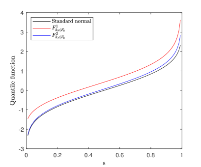
Figure EC.1: The supremum of $\mathcal{F}_{2,0.1}(F_{0})$ with $F_{0}\sim N(0,1)$.

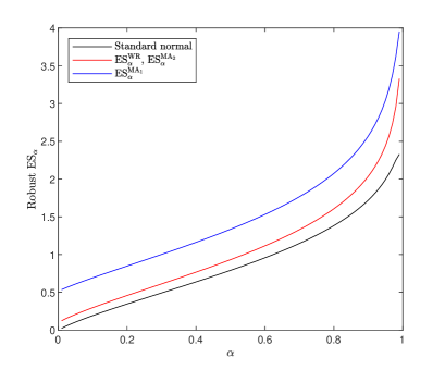
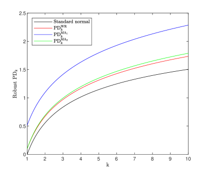
Figure EC.2: The WR and MA approaches under $\mathcal{F}_{2,0.1}(F_{0})$ with $F_{0}\sim N(0,1)$.

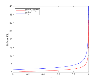
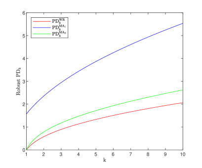
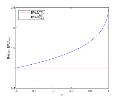
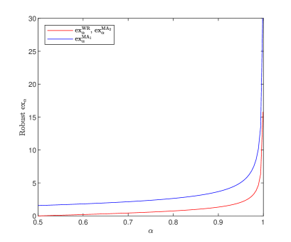
Figure EC.3: The WR and MA approaches under mean-variance uncertainty $\mathcal{F}_{0,1}$.

Appendix F Proofs and generalizations for results in Section 7

We first recall that, by Proposition 2, $\preceq_{1}$-cEMA and $\preceq_{2}$-cEMA imply the properties $\preceq_{1}$-consistency and $\preceq_{2}$-consistency, respectively, and $\preceq_{i}$-cEMA ($i=1,2$) is equivalent to

$$\rho\left(\bigvee_{i}\{F_{1},\dots,F_{n}\}\right)=\sup\left\{\rho\left(\sum_{i=1}^{n}\lambda_{i}F_{i}\right):\bm{\lambda}\in\Delta_{n}\right\}$$

for all $F_{1},\dots,F_{n}\in\mathcal{M}$ and $n\geqslant 1$.

F.1 A generalization of Theorem 6 (a) and related results

The following theorem is a generalized version of Theorem 6 (a) to the domain $\mathcal{M}_{p}$, $p\in[0,\infty)$.

Theorem EC.1.

Let $p\in[0,\infty)$. A mapping $\rho:\mathcal{M}_{p}\to\mathbb{R}$ satisfies translation invariance, positive homogeneity, lower semicontinuity and $\preceq_{1}$-cEMA if and only if $\rho=\mathrm{VaR}_{\alpha}$ for some $\alpha\in(0,1)$.

To prove Theorem EC.1, we need some technical lemmas. The following lemma shows that a $\preceq_{1}$-consistent and lower semicontinuous risk measure can be uniquely extended from $\mathcal{M}_{\infty}$ to $\mathcal{M}_{\rm bb}$.

Lemma EC.1.

Let $p\in[0,\infty)$ and $\rho_{1},\rho_{2}:\mathcal{M}_{p}\to\mathbb{R}\cup\{\infty\}$ be two $\preceq_{1}$-consistent and lower semicontinuous risk measures that coincide on $\mathcal{M}_{\infty}$. Then $\rho_{1}(F)=\rho_{2}(F)$ for all $F\in\mathcal{M}_{\rm bb}\cap\mathcal{M}_{p}$.

Proof.

For $F\in\mathcal{M}_{\rm bb}\cap\mathcal{M}_{p}$, without loss of generality assume that the support of $F$ is bounded from below by $-M$. Define $F_{n}(x)=\sum_{k=0}^{n2^{n}}F(k/2^{n}-M)\mathds{1}_{\{\frac{k-1}{2^{n}}\leqslant x+M<\frac{k}{2^{n}}\}}+\mathds{1}_{\{x+M\geqslant n\}},$ $n\in\mathbb{N}$. We have $F_{n}\in\mathcal{M}_{\infty}$, $F_{n}\preceq_{1}F_{n+1}$ for all $n\geqslant 1$, $F_{n}\buildrel\mathrm{d}\over{\rightarrow}F$ as $n\to\infty$, and

$$\rho_{1}(F)\geqslant\limsup_{n\to\infty}\rho_{1}(F_{n})=\limsup_{n\to\infty}\rho_{2}(F_{n})\geqslant\liminf_{n\to\infty}\rho_{2}(F_{n})\geqslant\rho_{2}(F),$$

where the first inequality follows from the $\preceq_{1}$-consistency of $\rho_{1}$, and the last inequality is due to the lower semicontinuity of $\rho_{2}$. By symmetry, we have $\rho_{1}=\rho_{2}$. ∎

Denote by $\ell$ the Lebesgue measure on $[0,1]$ and $\mathcal{M}_{1,f}(\ell)$ the space of all finitely additive probability measures on $([0,1],\mathfrak{B}([0,1]))$ that are absolutely continuous with respect to $\ell$. By Theorem 4.5 of Jia et al. (2020), for any $\preceq_{1}$-consistent, translation invariant and positively homogeneous risk measure $\rho:\mathcal{M}_{\infty}\to\mathbb{R}$, there exists a family $\{\mathcal{M}_{\xi}:\xi\in\Xi\}$ ($\Xi$ is an index set) of nonempty, ${\rm weak}^{*}$-compact and convex subsets of $\mathcal{M}_{1,f}(\ell)$ such that

$$\rho(F)=\min_{\xi\in\Xi}\max_{\mu\in\mathcal{M}_{\xi}}\int_{0}^{1}\mathrm{VaR}_{s}(F)\mu(\mathrm{d}s),~{}~{}F\in\mathcal{M}_{\infty}.$$ (EC.12)

Applying this representation, we can establish the following lemma.

Lemma EC.2.

Let $\rho:\mathcal{M}_{p}\to\mathbb{R}$, $p\in[0,\infty)$, be a mapping satisfying $\preceq_{1}$-consistency, translation invariance, positive homogeneity and lower semicontinuity. Denote by $\widehat{\rho}$ the restriction of $\rho$ on $\mathcal{M}_{\infty}$, i.e., $\widehat{\rho}(F)=\rho(F)$ for all $F\in\mathcal{M}_{\infty}$. Then the following three statements are equivalent.

• $\widehat{\rho}=\mathrm{VaR}_{\alpha}$ for some $\alpha\in(0,1)$ on $\mathcal{M}_{\infty}$.

• $\widehat{\rho}$ satisfies $\preceq_{1}$-cEMA.

• $\widehat{\rho}$ admits a representation (EC.12) which satisfies $\max_{\xi\in\Xi}\min_{\mu\in\mathcal{M}_{\xi}}\mu([0,s])=\mathds{1}_{\{s\geqslant\alpha\}}$ for some $\alpha\in(0,1)$.

Proof.

The implication (a)$\Rightarrow$(b) is straightforward to check by Proposition EC.1.

(b)$\Rightarrow$(c): By the discussion before this lemma, there exists a family $\{\mathcal{M}_{\xi}:\xi\in\Xi\}$ consisting of nonempty, ${\rm weak}^{*}$-compact and convex subsets of $\mathcal{M}_{1,f}(\ell)$ such that $\widehat{\rho}$ admits a representation (EC.12). Denote by

$$g_{\mu}(\beta)=\mu([0,\beta]),~{}\beta\in[0,1],~{}~{}g_{\xi}=\min_{\mu\in\mathcal{M}_{\xi}}g_{\mu}~{}~{}{\rm and}~{}~{}g_{\Xi}=\max_{\xi\in\Xi}g_{\xi}.$$

All these three functions are nonnegative, increasing, and take value one at $1$. We complete the proof of (b)$\Rightarrow$(c) by verifying the following three facts.

• Right-continuity of $g_{\Xi}$. Note that for any $\beta\in[0,1)$,

  $$\rho(\beta\delta_{0}+(1-\beta)\delta_{1}) =\min_{\xi\in\Xi}\max_{\mu\in\mathcal{M}_{\xi}}\int_{0}^{1}\mathrm{VaR}_{s}(\beta\delta_{0}+(1-\beta)\delta_{1})\mu(\mathrm{d}s)$$

  $$=\min_{\xi\in\Xi}\max_{\mu\in\mathcal{M}_{\xi}}\int_{(\beta,1]}1\mu(\mathrm{d}s)$$

  $$=\min_{\xi\in\Xi}\max_{\mu\in\mathcal{M}_{\xi}}\mu((\beta,1])=\min_{\xi\in\Xi}\max_{\mu\in\mathcal{M}_{\xi}}(1-g_{\mu}(\beta))=1-g_{\Xi}(\beta).$$ (EC.13)

  Fix $\beta\in[0,1)$. Let $\{\beta_{n}\}_{n\in\mathbb{N}}\subseteq[0,1)$ such that $\beta_{n}>\beta$ and $\beta_{n}\downarrow\beta$ as $n\to\infty$. We have $\beta_{n}\delta_{0}+(1-\beta_{n})\delta_{1}\preceq_{1}\beta\delta_{0}+(1-\beta)\delta_{1}$, $n\in\mathbb{N}$, and $\beta_{n}\delta_{0}+(1-\beta_{n})\delta_{1}\stackrel{{\scriptstyle\rm d}}{{\to}}\beta\delta_{0}+(1-\beta)\delta_{1}$ as $n\to\infty$. Therefore, by (EC.13), we have

  $$\limsup_{n\to\infty}\{1-g_{\Xi}(\beta_{n})\}=\limsup_{n\to\infty}\rho(\beta_{n}\delta_{0}+(1-\beta_{n})\delta_{1})\leqslant\rho(\beta\delta_{0}+(1-\beta)\delta_{1})=1-g_{\Xi}(\beta),$$

  where the inequality comes from $\beta_{n}\delta_{0}+(1-\beta_{n})\delta_{1}\preceq_{1}\beta\delta_{0}+(1-\beta)\delta_{1}$ and $\preceq_{1}$-consistency of $\rho$. By lower semicontinuity of $\rho$, we have

  $$\liminf_{n\to\infty}\{1-g_{\Xi}(\beta_{n})\}=\liminf_{n\to\infty}\rho(\beta_{n}\delta_{0}+(1-\beta_{n})\delta_{1})\geqslant\rho(\beta\delta_{0}+(1-\beta)\delta_{1})=1-g_{\Xi}(\beta).$$

  Hence, we obtain $g_{\Xi}(\beta)=\lim_{n\to\infty}g_{\Xi}(\beta_{n})$ which implies the right-continuity of $g_{\Xi}$.

• $g_{\Xi}(1-)=g_{\Xi}(1)=1$. Assume by contradiction that $g_{\Xi}(1-)=1-\delta$ with $\delta\in(0,1]$. By the definition of $g_{\Xi}$, we obtain that for all $\xi\in\Xi$, there exists $\mu\in\mathcal{M}_{\xi}$ such that $g_{\mu}(1-)\leqslant g_{\Xi}(1-)=1-\delta$. Take $G\in\mathcal{M}_{p}\setminus\mathcal{M}_{\infty}$, $p\in[0,\infty)$ with support on $\mathbb{R}_{+}$. For any $M\in\mathbb{R}_{+}$, take $\beta=G(M)\in[0,1)$ and define $F:=\beta\delta_{0}+(1-\beta)\delta_{M}\in\mathcal{M}_{\infty}$. One can verify that $F\geqslant G$ and thus, $F\preceq_{1}G$. Therefore,

  $$\rho(G)\geqslant\rho(F)=\widehat{\rho}(F)=\min_{\xi\in\Xi}\max_{\mu\in\mathcal{M}_{\xi}}\int_{0}^{1}\mathrm{VaR}_{s}(F)\mu(\mathrm{d}s)=M(1-g_{\Xi}(\beta))\geqslant\delta M,$$

  where the last inequality follows from $g_{\Xi}(\beta)\leqslant g_{\Xi}(1-)=1-\delta$ for any $\beta<1$. Since $M$ is arbitrary, this yields a contradiction to that $\rho:\mathcal{M}_{p}\to\mathbb{R}$, $p\in[0,\infty)$.

• $g_{\Xi}(\beta)=\mathds{1}_{\{\beta\geqslant\alpha\}}$ for some $\alpha\in(0,1)$. Define

  $$\alpha=\inf\left\{\beta:g_{\Xi}(\beta)>0\right\}\in[0,1].$$ (EC.14)

  We assert $\alpha\in(0,1)$. To see this, first note that $g_{\Xi}(1-)=1$ which implies $\alpha<1$. We next show $\alpha>0$ by contradiction. Suppose that $\alpha=0$, which means $g_{\Xi}(\beta)>0$ for each $\beta>0$. Let $F=\beta\delta_{-a}+(1-\beta)\delta_{1}$ and $G=\delta_{0}$ with $\beta\in(0,1)$ and $a>0$. We can calculate the MA robust risk value

  $$\widehat{\rho}\left(\bigvee_{1}\{F,G\}\right)=\widehat{\rho}(\beta\delta_{0}+(1-\beta)\delta_{1})=1-g_{\Xi}(\beta),$$

  and the WR robust risk value

  $$\sup_{\lambda\in[0,1]}\widehat{\rho}\left(\lambda F+(1-\lambda)G\right) =\sup_{\lambda\in[0,1]}\widehat{\rho}(\lambda\beta\delta_{-a}+(1-\lambda)\delta_{0}+\lambda(1-\beta)\delta_{1})$$

  $$=\sup_{\lambda\in[0,1]}\min_{\xi\in\Xi}\max_{\mu\in\mathcal{M}_{\xi}}\{-ag_{\mu}(\lambda\beta)+1-g_{\mu}(1-\lambda(1-\beta))\}$$

  $$=1-\inf_{\lambda\in[0,1]}\max_{\xi\in\Xi}\min_{\mu\in\mathcal{M}_{\xi}}\{ag_{\mu}(\lambda\beta)+g_{\mu}(1-\lambda(1-\beta))\}$$

  $$\leqslant 1-\inf_{\lambda\in[0,1]}\max_{\xi\in\Xi}\{a\min_{\mu\in\mathcal{M}_{\xi}}g_{\mu}(\lambda\beta)+\min_{\mu\in\mathcal{M}_{\xi}}g_{\mu}(1-\lambda(1-\beta))\}$$

  $$=1-\inf_{\lambda\in[0,1]}\max_{\xi\in\Xi}\{a\,g_{\xi}(\lambda\beta)+g_{\xi}(1-\lambda(1-\beta))\}.$$

  The property $\preceq_{1}$-cEMA implies $\widehat{\rho}\left(\bigvee_{1}\{F,G\}\right)=\sup_{\lambda\in[0,1]}\widehat{\rho}\left(\lambda F+(1-\lambda)G\right)$, and thus,

  $$g_{\Xi}(\beta)\geqslant\inf_{\lambda\in[0,1]}\max_{\xi\in\Xi}\{a\,g_{\xi}(\lambda\beta)+g_{\xi}(1-\lambda(1-\beta))\},~{}~{}\beta\in[0,1],~{}a>0.$$ (EC.15)

  Fix $\beta>0$. By (EC.15) and the definition of infimum, for each $a>0$, there exist $\varepsilon_{a}$ and $\lambda_{a}\in[0,1]$ such that $\lim_{a\to\infty}{\varepsilon_{a}}=0$ and

  $$g_{\Xi}(\beta)\geqslant\max_{\xi\in\Xi}\{a\,g_{\xi}(\lambda_{a}\beta)+g_{\xi}(1-\lambda_{a}(1-\beta))\}-\varepsilon_{a}.$$ (EC.16)

  It follows that $g_{\Xi}(\beta)\geqslant\max_{\xi\in\Xi}a\,g_{\xi}(\lambda_{a}\beta)-\varepsilon_{a}=a\,g_{\Xi}(\lambda_{a}\beta)-\varepsilon_{a}$ which implies $g_{\Xi}(\lambda_{a}\beta)\to 0$ as $a\to\infty$. That is, $\lambda_{a}\to 0$ as $a\to\infty$ since $g(\beta)>0$ for $\beta>0$. Therefore, (EC.16) implies $g_{\Xi}(\beta)\geqslant\max_{\xi\in\Xi}g_{\xi}(1-\lambda_{a}(1-\beta))-\varepsilon_{a}=g_{\Xi}(1-\lambda_{a}(1-\beta))-\varepsilon_{a}.$ Letting $a\to\infty$, we have $g_{\Xi}(\beta)\geqslant g_{\Xi}(1-)=1$ for any $\beta>0$ which implies $g_{\Xi}(s)=\mathds{1}_{\{s>0\}}$ for $s\in[0,1]$, and this yields a contradiction to that $g$ is right-continuous on $[0,1)$. Hence, we have $\alpha>0$, and thus, $\alpha\in(0,1)$. By the definition of $\alpha$ in (EC.14), we have $g_{\Xi}(\beta)=0$ for all $\beta\in[0,\alpha)$. Fix $\beta>\alpha$, there exist $\varepsilon_{a}$ and $\lambda_{a}\in[0,1]$ such that $\lim_{a\to\infty}{\varepsilon_{a}}=0$ and (EC.16) holds. Similarly, we have $g_{\Xi}(\lambda_{a}\beta)\to 0$ as $a\to\infty$ which implies $\limsup_{a\to\infty}\lambda_{a}\leqslant\alpha/\beta$. It then follows that $g_{\Xi}(\beta)\geqslant g_{\Xi}(1-\lambda_{a}(1-\beta))-\varepsilon_{a}.$ Letting $a\to\infty$, we have

  $$g_{\Xi}(\beta)\geqslant\limsup_{a\to\infty}g_{\Xi}(1-\lambda_{a}(1-\beta))\geqslant g_{\Xi}\left(\left(1-\frac{\alpha(1-\beta)}{\beta}\right)-\right).$$

  Since $\beta<1-\alpha(1-\beta)/\beta$ for $\beta>\alpha$, and the sequence $\{\beta_{n}\}_{n\in\mathbb{N}}$, where $\beta_{0}=\beta$ and $\beta_{n+1}=1-\alpha(1-\beta_{n})/\beta_{n}$ for $n\geqslant 0$, converges to 1, and $g_{\Xi}$ is increasing, we have $g_{\Xi}(\beta)$ takes constant on $\beta\in(\alpha,1)$, that is, $g_{\Xi}(\beta)=g_{\Xi}(1-)=1$. By right-continuity of $g_{\Xi}$, we have $g_{\Xi}(\beta)=\mathds{1}_{\{\beta\geqslant\alpha\}}$, which completes the proof of (b)$\Rightarrow$(c).

(c)$\Rightarrow$(a): By (EC.13), under the condition of (c), for $F=\beta\delta_{0}+(1-\beta)\delta_{1}$, we have $\rho(F)=1-g_{\Xi}(\beta)={\rm VaR}_{\alpha}(F)$. By positive homogeneity and translation invariance of $\rho$, this implies that for any $F=\beta\delta_{a}+(1-\beta)\delta_{b}$,

$$\rho(F)=a+(b-a)\min_{\xi\in\Xi}\max_{\mu\in\mathcal{M}_{\xi}}\mu((\beta,1])=a+(b-a){\rm VaR}_{\alpha}(\beta\delta_{0}+(1-\beta)\delta_{1})={\rm VaR}_{\alpha}(F),$$

where the second equality follows from $\min_{\xi\in\Xi}\max_{\mu\in\mathcal{M}_{\xi}}\mu((\beta,1])=1-\max_{\xi\in\Xi}\min_{\mu\in\mathcal{M}_{\xi}}\mu([0,\beta])=\mathds{1}_{\{s<\alpha\}}.$

For $F\in\mathcal{M}_{\infty}$, define $G=\beta\delta_{{\rm VaR}_{0}(F)}+(1-\beta)\delta_{{\rm VaR}_{\beta}(F)}$ for $\beta<\alpha$. One can check $G\preceq_{1}F$ and thus, $\rho(F)\geqslant\rho(G)={\rm VaR}_{\alpha}(G)={\rm VaR}_{\beta}(F)$ for $\beta<\alpha$. By left-continuity of ${\rm VaR}$, we have $\rho(F)\geqslant\lim_{\beta\uparrow\alpha}\mathrm{VaR}_{\beta}(F)={\rm VaR}_{\alpha}(F)$. On the other hand, define $H=\alpha\delta_{{\rm VaR}_{\alpha}(F)}+(1-\alpha)\delta_{{\rm VaR}_{1}(F)}$. One can check $F\preceq_{1}H$ and thus, $\rho(F)\leqslant\rho(H)={\rm VaR}_{\alpha}(H)={\rm VaR}_{\alpha}(F)$. Therefore, we have $\rho(F)={\rm VaR}_{\alpha}(F)$. ∎

Proof of Theorem EC.1.  Sufficiency follows directly from Proposition EC.1. Below we show necessity. Note that $\preceq_{1}$-cEMA implies $\preceq_{1}$-consistency, and hence, by Lemma EC.2, we have $\rho=\mathrm{VaR}_{\alpha}$ for some $\alpha\in(0,1)$ on $\mathcal{M}_{\infty}$. It remains to show that $\rho=\mathrm{VaR}_{\alpha}$ on $\mathcal{M}_{p}$, $p\in[0,\infty)$. By Lemma EC.1, we have $\rho=\mathrm{VaR}_{\alpha}$ on $\mathcal{M}_{\rm bb}\cap\mathcal{M}_{p}$. Next, we will prove $\rho=\mathrm{VaR}_{\alpha}$ on $\mathcal{M}_{p}\setminus\mathcal{M}_{\rm bb}$. Take $F\in\mathcal{M}_{p}\setminus\mathcal{M}_{\rm bb}$ and $\zeta<\mathrm{VaR}_{\alpha}(F)$. We have

$$\rho\left(\bigvee_{1}\{F,\delta_{\zeta}\}\right)=\mathrm{VaR}_{\alpha}\left(\bigvee_{1}\{F,\delta_{\zeta}\}\right)=\mathrm{VaR}_{\alpha}(F)\vee\zeta=\mathrm{VaR}_{\alpha}(F),$$ (EC.17)

where the first equality is due to $\bigvee_{1}\{F,\delta_{\zeta}\}\in\mathcal{M}_{\rm bb}\cap\mathcal{M}_{p}$ and the second equality follows from Proposition EC.1. By $F\preceq_{1}\bigvee_{1}\{F,\delta_{\zeta}\}$ and $\preceq_{1}$-consistency, we have (EC.17) implies that

$$\rho(F)\leqslant\mathrm{VaR}_{\alpha}(F)~{}{\rm for~{}all}~{}F\in\mathcal{M}_{p}\setminus\mathcal{M}_{\rm bb}.$$ (EC.18)

By $\preceq_{1}$-cEMA of $\rho$, and together with (EC.17), we have

$$\sup_{0\leqslant\lambda\leqslant 1}\rho(\lambda F+(1-\lambda)\delta_{\zeta})=\mathrm{VaR}_{\alpha}(F)~{}~{}{\rm for~{}}\zeta<\mathrm{VaR}_{\alpha}(F).$$ (EC.19)

We assert that if $F$ is continuous at $\mathrm{VaR}_{\alpha}(F)$, then (EC.19) implies

$$\limsup_{\lambda\to 1}\rho(\lambda F+(1-\lambda)\delta_{\zeta})=\mathrm{VaR}_{\alpha}(F),~{}~{}~{}\zeta<\mathrm{VaR}_{\alpha}(F).$$ (EC.20)

To see this, fix $\varepsilon>0$ and $\zeta<\mathrm{VaR}_{\alpha}(F)$, and let $\lambda\in[0,1-\varepsilon)$. Since $F$ is continuous at $\mathrm{VaR}_{\alpha}(F)$, we have $\zeta^{\prime}:=\mathrm{VaR}_{(\alpha-\varepsilon)/(1-\varepsilon)}(F)<\mathrm{VaR}_{\alpha}(F)$. Hence, $\lambda F+(1-\lambda)\delta_{\zeta}$ has probability at least $\alpha-\varepsilon+\varepsilon\geqslant\alpha$ for the interval $(-\infty,\zeta^{\prime}\vee\zeta]$. Therefore, we have $\mathrm{VaR}_{\alpha}(\lambda F+(1-\lambda)\delta_{\zeta})\leqslant\zeta^{\prime}\vee\zeta<\mathrm{VaR}_{\alpha}(F)$. Hence,

$$\sup_{0\leqslant\lambda\leqslant 1-\varepsilon}\rho(\lambda F+(1-\lambda)\delta_{\zeta})\leqslant\zeta^{\prime}\vee\zeta<\mathrm{VaR}_{\alpha}(F).$$

Therefore, the supremum in (EC.19) is not attained on $[0,1-\varepsilon)$ for any $\varepsilon>0$, and we have

$$\limsup_{\lambda\to 1}\rho(\lambda F+(1-\lambda)\delta_{\zeta})\vee\rho(F)=\mathrm{VaR}_{\alpha}(F),~{}~{}~{}\zeta<\mathrm{VaR}_{\alpha}(F).$$

By lower semicontinuity of $\rho$, we have

$$\rho(F)\leqslant\liminf_{\lambda\to 1}\rho(\lambda F+(1-\lambda)\delta_{\zeta})\leqslant\limsup_{\lambda\to 1}\rho(\lambda F+(1-\lambda)\delta_{\zeta}).$$

Combining above two equations, the assertion (EC.20) is verified. In the following, we will show that $\rho(G)=\mathrm{VaR}_{\alpha}(G)$ for $G\in\mathcal{M}_{p}\setminus\mathcal{M}_{\rm bb}$ in two cases by applying (EC.18) and (EC.20).
Case 1: $G$ is continuous at $\mathrm{VaR}_{\alpha}(G)$. By (EC.18), $\rho(G)\leqslant\mathrm{VaR}_{\alpha}(G)$, and we suppose by contradiction that $\rho(G)<\mathrm{VaR}_{\alpha}(G)$. Since $G$ is continuous at $\mathrm{VaR}_{\alpha}(G)$, there exist $x^{*}\in(\rho(G),\mathrm{VaR}_{\alpha}(G))$ such that $G$ is continuous at $x^{*}$, and $x^{*}$ is an element of the support of $G$, which implies $\mathrm{VaR}_{G(x^{*})}(G)=x^{*}$. Noting that $x^{*}<\mathrm{VaR}_{\alpha}(G)$, we have $\lambda^{*}:=G(x^{*})/\alpha\in(0,1)$. Define a cdf as

$$H(x)=\begin{cases}\frac{1}{\lambda^{*}}G(x)\wedge 1,~{}~{}~{}&x<\mathrm{VaR}_{\alpha}(G)\\ 1,~{}~{}~{}&x\geqslant\mathrm{VaR}_{\alpha}(G).\end{cases}$$

One can check that $H$ is continuous at $x^{*}$ and $\mathrm{VaR}_{\alpha}(H)=x^{*}$. By (EC.20), we obtain for $\zeta<x^{*}$,

$$\limsup_{\lambda\to 1}\rho(\lambda H+(1-\lambda)\delta_{\zeta})=\mathrm{VaR}_{\alpha}(H)=x^{*}.$$ (EC.21)

For $\zeta<x^{*}$ and $\lambda\in[\lambda^{*},1]$, we have $\lambda H+(1-\lambda)\delta_{\zeta}\geqslant G$ pointwise, which implies $\lambda H+(1-\lambda)\delta_{\zeta}\preceq_{1}G$. It follows from $\preceq_{1}$-consistency that $\rho(G)\geqslant\rho(\lambda H+(1-\lambda)\delta_{\zeta})$ for all $\zeta<x^{*}$ and $\lambda\in[\lambda^{*},1]$. Hence, by (EC.21), we obtain $\rho(G)\geqslant x^{*}$, and this yields a contradiction.
Case 2: $G$ has a jump at $\mathrm{VaR}_{\alpha}(G)$. In this case, we can construct a sequence $\{G_{n}\}_{n\in\mathbb{N}}$ such that $G_{n}\preceq_{1}F$ for all $n\in\mathbb{N}$, $G_{n}$ is continuous at point $\mathrm{VaR}_{\alpha}(G_{n})$ and $\mathrm{VaR}_{\alpha}(G_{n})\to\mathrm{VaR}_{\alpha}(G)$. By Case 1 and $\preceq_{1}$-consistency of $\rho$, we have $\rho(G)\geqslant\rho(G_{n})\to\mathrm{VaR}_{\alpha}(G)$. Note that the converse direction holds by (EC.18). Hence, we obtain $\rho(G)=\mathrm{VaR}_{\alpha}(G)$ for all $F\in\mathcal{M}_{p}\setminus\mathcal{M}_{\rm bb}$ such that $G$ has a jump at point $\zeta$.

In summary, we compete the proof of this theorem.∎

F.2 A generalization of Theorem 6 (b) and related results

The following theorem is a generalized result of Theorem 6 (b) for the space $\mathcal{M}_{p}$, $p\in[1,\infty)$.

Theorem EC.2.

A mapping $\rho:\mathcal{M}_{p}\to\mathbb{R}$, $p\in[1,\infty)$, satisfies translation invariance, positive homogeneity, lower semicontinuity and $\preceq_{2}$-cEMA if and only if $\rho=\mathrm{ES}_{\alpha}$ for some $\alpha\in(0,1)$.

By Theorem 1, we know that $\mathrm{ES}$ satisfies $\preceq_{2}$-cEMA. In order to prove the necessity of Theorem EC.2, we need to apply Corollary 5.9 of Jia et al. (2020). Define

$$\mathcal{H}:=\{h:[0,1]\to[0,1]:~{}h~{}{\rm is~{}increasing~{}convex},~{}h(0)=0,~{}h(1)=1\}.$$

For any $\preceq_{2}$-consistent, translation invariant and positively homogeneous risk measure $\rho:\mathcal{M}_{\infty}\to\mathbb{R}$, there exists a family $\{\mathcal{H}_{\xi}:\xi\in\Xi\}$ of nonempty, compact and convex subsets of $\mathcal{H}$ such that

$$\rho(F)=\min_{\xi\in\Xi}\max_{h\in\mathcal{H}_{\xi}}\int_{0}^{1}\mathrm{VaR}_{s}(F)\mathrm{d}h(s),~{}~{}F\in\mathcal{M}_{\infty}.$$ (EC.22)

Here, compactness is defined with respect to the weak topology induced by all continuous functions on $[0,1]$. As pointed out by Jia et al. (2020), both the $\min$ and $\max$ can be attained, that is, for each $F\in\mathcal{M}_{\infty}$, there exists $h\in\mathcal{H}_{\xi}$ for some $\xi\in\Xi$ such that $\rho(F)=\int_{0}^{1}\mathrm{VaR}_{s}(F)\mathrm{d}h(s)$. Therefore, for any $\beta\in[0,1]$, by $\rho(\beta\delta_{0}+(1-\beta)\delta_{1})=\min_{\xi\in\Xi}\max_{h\in\mathcal{H}_{\xi}}\int_{\beta}^{1}1\mathrm{d}h(s)=1-\max_{\xi\in\Xi}\min_{h\in\mathcal{H}_{\xi}}h(\beta),$ we can define

$$h_{\xi}(\beta)=\min_{h\in\mathcal{H}_{\xi}}h(\beta)~{}~{}{\rm and}~{}~{}h_{\Xi}(\beta)=\max_{\xi\in\Xi}h_{\xi}(\beta),~{}~{}\beta\in[0,1].$$ (EC.23)

Applying this representation, we can establish the following lemma.

Lemma EC.3.

Let $\rho:\mathcal{M}_{p}\to\mathbb{R}$, $p\in[1,\infty)$, be a mapping satisfying $\preceq_{2}$-consistency, translation invariance and positive homogeneity. Denote by $\widehat{\rho}$ the restriction of $\rho$ on $\mathcal{M}_{\infty}$. Then the following three statements are equivalent.

• $\widehat{\rho}=\mathrm{ES}_{\alpha}$ for some $\alpha\in[0,1)$ on $\mathcal{M}_{\infty}$.

• $\widehat{\rho}$ satisfies $\preceq_{2}$-cEMA.

• $\widehat{\rho}$ admits a representation (EC.22) which satisfies $h_{\Xi}(\beta)=(\beta-\alpha)_{+}/(1-\alpha)$ for some $\alpha\in[0,1)$ where $h_{\Xi}$ is defined by (EC.23).

Proof.

The implication (a)$\Rightarrow$(b) follows immediately from Theorem 1 (b).

(b)$\Rightarrow$(c): By the discussion before this lemma, there exists a family $\{\mathcal{H}_{\xi}:\xi\in\Xi\}$ of nonempty, compact and convex subsets of $\mathcal{H}$ such that $\widehat{\rho}$ admits a representation (EC.22). Define $h_{\xi}$ and $h_{\Xi}$ by (EC.23). One can check that both $h_{\xi}$ and $h_{\Xi}$ are increasing and satisfy $h_{\xi}(0)=h_{\Xi}(0)=0$ and $h_{\xi}(1)=h_{\Xi}(1)=1.$ In the following, we show (c) by verifying the following facts.
1. $h_{\Xi}(1-)=h_{\Xi}(1)=1$. This can be showed by similar arguments as in (b)$\Rightarrow$(c) of Lemma EC.2.
2. $h_{\Xi}(\beta)=(\beta-\alpha)_{+}/(1-\alpha)$ for some $\alpha\in[0,1)$. Let $F=\beta\delta_{-a}+(1-\beta)\delta_{1}$ and $G=\delta_{0}$ with $\beta\in(0,1)$ and $a>(1-\beta)/\beta$, and calculate the MA robust risk value

$$\widehat{\rho}\left(\bigvee_{2}\{F,G\}\right)=\widehat{\rho}\left(\beta\delta_{-\frac{1-\beta}{\beta}}+(1-\beta)\delta_{1}\right)=1-\frac{h_{\Xi}(\beta)}{\beta},$$

and the WR robust risk value

$$\sup_{\lambda\in[0,1]}\widehat{\rho}\left(\lambda F+(1-\lambda)G\right) =\sup_{\lambda\in[0,1]}\widehat{\rho}(\lambda\beta\delta_{-a}+(1-\lambda)\delta_{0}+\lambda(1-\beta)\delta_{1})$$

$$=\sup_{\lambda\in[0,1]}\min_{\xi\in\Xi}\max_{h\in\mathcal{H}_{\xi}}\{-a\,h(\lambda\beta)+1-h(1-\lambda(1-\beta))\}$$

$$=1-\inf_{\lambda\in[0,1]}\max_{\xi\in\Xi}\min_{h\in\mathcal{H}_{\xi}}\{a\,h(\lambda\beta)+h(1-\lambda(1-\beta))\}$$

$$\leqslant 1-\inf_{\lambda\in[0,1]}\max_{\xi\in\Xi}\{a\,\min_{h\in\mathcal{H}_{\xi}}h(\lambda\beta)+\min_{h\in\mathcal{H}_{\xi}}h(1-\lambda(1-\beta))\}$$

$$=1-\inf_{\lambda\in[0,1]}\max_{\xi\in\Xi}\{a\,h_{\xi}(\lambda\beta)+h_{\xi}(1-\lambda(1-\beta))\}.$$

The property $\preceq_{2}$-cEMA implies $\sup_{\lambda\in[0,1]}\widehat{\rho}\left(\lambda F+(1-\lambda)G\right)=\widehat{\rho}\left(\bigvee_{2}\{F,G\}\right)$, and thus,

$$\frac{h_{\Xi}(\beta)}{\beta}\geqslant\inf_{\lambda\in[0,1]}\max_{\xi\in\Xi}\{a\,h_{\xi}(\lambda\beta)+h_{\xi}(1-\lambda(1-\beta))\},~{}~{}\beta\in[0,1],~{}a>\frac{1-\beta}{\beta}.$$ (EC.24)

Define

$$\alpha=\inf\left\{\beta:h_{\Xi}(\beta)>0\right\}\in[0,1),$$ (EC.25)

where the fact $\alpha<1$ comes from $h_{\Xi}(1-)=1$. Fix $\beta>\alpha$. By (EC.24) and the definition of infimum, for each $a>{(1-\beta)}/{\beta}$, there exist $\lambda_{a}\in[0,1]$ and $\varepsilon_{a}$ such that $\lim_{a\to\infty}\varepsilon_{a}=0$ and

$$\frac{h_{\Xi}(\beta)}{\beta}\geqslant\max_{\xi\in\Xi}\{ah_{\xi}(\lambda_{a}\beta)+h_{\xi}(1-\lambda_{a}(1-\beta))\}-\varepsilon_{a}.$$ (EC.26)

It follows that ${h_{\Xi}(\beta)}/{\beta}\geqslant\max_{\xi\in\Xi}a\,h_{\xi}(\lambda_{a}\beta)-\varepsilon_{a}=a\,h_{\Xi}(\lambda_{a}\beta)-\varepsilon_{a}.$ Letting $a\to\infty$, we obtain $\lim_{a\to\infty}h_{\Xi}(\lambda_{a}\beta)=0$. By definition of $\alpha$, $\limsup_{a\to\infty}\lambda_{a}\leqslant\alpha/\beta.$ Again, by (EC.26), we have

$$\frac{h_{\Xi}(\beta)}{\beta} \geqslant\max_{\xi\in\Xi}\{h_{\xi}(1-\lambda_{a}(1-\beta))\}-\varepsilon_{a}=h_{\Xi}(1-\lambda_{a}(1-\beta))-\varepsilon_{a}$$ (EC.27)

By monotonicity of $h_{\Xi}$ and $\limsup_{a\to\infty}\lambda_{a}\leqslant\alpha/\beta$, we get $\limsup_{a\to\infty}h_{\Xi}(1-\lambda_{a}(1-\beta))-\varepsilon_{a}\geqslant h_{\Xi}((1-\alpha(1-\beta)/\beta)-)$. This combined with (EC.27) implies ${h_{\Xi}(\beta)}/{\beta}\geqslant h_{\Xi}((1-\alpha(1-\beta)/\beta)-).$ Denote by $h_{\Xi}^{-}(x)=\lim_{y\uparrow x}h_{\Xi}(y)$. We have $h_{\Xi}^{-}(\alpha)=0$ and

$$\frac{h_{\Xi}^{-}(\beta)-h_{\Xi}^{-}(\alpha)}{\beta-\alpha}\geqslant\frac{h_{\Xi}^{-}(\alpha+(1-\alpha/\beta))-h_{\Xi}^{-}(\alpha)}{1-\alpha/\beta},~{}~{}\beta>\alpha.$$ (EC.28)

Letting $\beta_{0}=\beta$ and $\beta_{n+1}=1+\alpha-\alpha/\beta_{n}$ for $n\geqslant 0$, we have $\beta_{n}=\frac{\alpha(1-\beta)+(\beta-\alpha)\alpha^{-n+1}}{(1-\beta)+(\beta-\alpha)\alpha^{-n+1}}\uparrow 1$ as $n\to\infty$. Combining with (EC.28), we obtain

$$\frac{h_{\Xi}^{-}(\beta)-h_{\Xi}^{-}(\alpha)}{\beta-\alpha}\geqslant\frac{h_{\Xi}^{-}(\beta_{n})-h_{\Xi}^{-}(\alpha)}{\beta_{n}-\alpha}\to\frac{h_{\Xi}^{-}(1)-h_{\Xi}^{-}(\alpha)}{1-\alpha}=\frac{1}{1-\alpha}~{}~{}{\rm as}~{}~{}n\to\infty$$

for all $\beta\in(\alpha,1]$. It follows that $h_{\Xi}(\beta)\geqslant h_{\Xi}^{-}(\beta)\geqslant(\beta-\alpha)_{+}/(1-\alpha)$ for $\beta\in(\alpha,1]$. We next show $h_{\Xi}(\beta)\leqslant(\beta-\alpha)_{+}/(1-\alpha)$ for $\beta\in(\alpha,1]$ by contradiction. Suppose that there exists $\beta^{*}\in(\alpha,1)$ such that $h_{\Xi}(\beta^{*})>(\beta^{*}-\alpha)_{+}/(1-\alpha)$. Noting that $h_{\Xi}(\beta)=\max_{\xi\in\Xi}\min_{h\in\mathcal{H}_{\xi}}h(\beta)$, there exists $\xi_{0}\in\Xi$ such that

$$\min_{h\in\mathcal{H}_{\xi_{0}}}h(\beta^{*})>\frac{(\beta^{*}-\alpha)_{+}}{1-\alpha}.$$ (EC.29)

Meanwhile, by $h_{\Xi}(\beta)=0$ for $\beta<\alpha$, we have $\min_{h\in\mathcal{H}_{\xi}}h(\beta)=0$ for any $\beta<\alpha$ and any $\xi\in\Xi$, and thus, $\min_{h\in\mathcal{H}_{\xi_{0}}}h(\beta)=0$ for $\beta<\alpha$. This implies that there exists $h_{0}\in\mathcal{H}_{\xi_{0}}$ such that $h_{0}(\beta)=0$ for $\beta<\alpha$. By (EC.29), we have $h_{0}(\beta^{*})>(\beta^{*}-\alpha)_{+}/(1-\alpha)$, which, combined with $h_{0}(1)=1$ and $h_{0}(\beta)=0$ for $\beta<\alpha$, yields a contradiction to that $h_{0}\in\mathcal{H}$ is convex. Hence, $h_{\Xi}(\beta)=(\beta-\alpha)_{+}/(1-\alpha)$, and this completes the proof of (b)$\Rightarrow$(c).

(c)$\Rightarrow$(a): One can check that under the condition of (c), for $F=\beta\delta_{0}+(1-\beta)\delta_{1}$, we have $\rho(F)=1-h_{\Xi}(\beta)={\rm ES}_{\alpha}(F)$. By positive homogeneity and translation invariance of $\rho$, for any $F=\beta\delta_{a}+(1-\beta)\delta_{b}$, $\rho(F)={\rm ES}_{\alpha}(F)$. For $F\in\mathcal{M}_{\infty}$, define $G=\alpha\delta_{{\rm VaR}_{0}(F)}+(1-\alpha)\delta_{{\rm ES}_{\alpha}(F)}$. By computing the $\pi$ function, one can check $G\preceq_{2}F$ and thus, $\rho(F)\geqslant\rho(G)={\rm ES}_{\alpha}(G)={\rm ES}_{\alpha}(F)$. On the other hand, define $H=\beta\delta_{{\rm VaR}_{\alpha}(F)}+(1-\beta)\delta_{{\rm VaR}_{1}(F)}$, where $\beta>\alpha$ satisfies $(\beta-\alpha){\rm VaR}_{\alpha}(F)+(1-\beta){\rm VaR}_{1}(F)=(1-\alpha){\rm ES}_{\alpha}(F)$, that is, ${\rm ES}_{\alpha}(H)={\rm ES}_{\alpha}(F)$. By computing the ES_s, $s\in[0,1]$, one can check $F\preceq_{2}H$ and thus, $\rho(F)\leqslant\rho(H)={\rm ES}_{\alpha}(H)={\rm ES}_{\alpha}(F)$. We therefore have $\rho(F)={\rm ES}_{\alpha}(F)$, which completes the proof. ∎

Proof of Theorem EC.2.  Translation invariance, positive homogeneity and lower semicontinuity of $\mathrm{ES}_{\alpha}$, $\alpha\in(0,1)$, are well-known, and the property $\preceq_{2}$-cEMA of $\mathrm{ES}$ follows from Theorem 1. Conversely, note that $\preceq_{2}$-cEMA implies $\preceq_{2}$-consistency, and hence, by Lemma EC.3, we have $\rho=\mathrm{ES}_{\alpha}$ for some $\alpha\in[0,1)$ on $\mathcal{M}_{\infty}$. Thus, it remains to show that this representation can be extended to $\mathcal{M}_{p}$ for $p\in[1,\infty)$. To see this, for $F\in\mathcal{M}_{p}$, let $X$ be a random variable with cdf $F$. Since the probability space is nonatomic, there exists a uniform random variable $U$ on $[0,1]$ such that $X=F^{-1}(U)$ $\mathbb{P}$-a.s. (see, e.g., Lemma A.28 of Föllmer and Schied (2016)). Define

$$U_{n}=\sum_{i=0}^{n-1}\frac{\alpha i}{n}\mathds{1}_{\left\{\frac{\alpha i}{n}\leqslant U<\frac{\alpha(i+1)}{n}\right\}}+\sum_{i=0}^{n-1}\left(\alpha+\frac{(1-\alpha)i}{n}\right)\mathds{1}_{\left\{\alpha+\frac{(1-\alpha)i}{n}\leqslant U<\alpha+\frac{(1-\alpha)(i+1)}{n}\right\}},~{}~{}n\geqslant 1.$$

and denote by $X_{n}=\mathbb{E}[X|U_{n}]$. One can obatin $F_{X_{n}}\in\mathcal{M}_{\infty}$, and $\rho(F_{X_{n}})=\mathrm{ES}_{\alpha}(F_{X_{n}})=\mathrm{ES}_{\alpha}(F)$. On one hand, since $F_{X_{n}}\preceq_{2}F$ for all $n\geqslant 1$, and note that $\preceq_{2}$-cEMA implies $\preceq_{2}$-consistency, we have $\rho(F_{X_{n}})\leqslant\rho(F)$. Hence, we have $\mathrm{ES}_{\alpha}(F)=\limsup_{n\to\infty}\rho(F_{X_{n}})\leqslant\rho(F)$. On the other hand, noting that $X_{n}\stackrel{{\scriptstyle\rm d}}{{\to}}X$, it follows from the lower semicontinuitycof $\rho$ that $\mathrm{ES}_{\alpha}(F)=\liminf_{n\to\infty}\rho(F_{X_{n}})\geqslant\rho(F)$. Hence, we conclude that $\rho(F)=\mathrm{ES}_{\alpha}(F)$. Since $\mathrm{ES}_{0}=\mathbb{E}$ is not lower semicontinuous, we obtain $\rho=\mathrm{ES}_{\alpha}$ for some $\alpha\in(0,1)$. ∎

Remark EC.3.

The characterization results in Theorems EC.1 and EC.2 are obtained for spaces $\mathcal{M}_{p}$, $p\in[1,\infty)$, i.e., cdfs with finite $p$th moment. On the space $\mathcal{M}_{\infty}$ of compactly supported cdfs, the situation is more delicate. In particular, for $\alpha\in(0,1)$ and $\lambda\in(0,1)$, we find that the mappings $\lambda\mathrm{VaR}_{\alpha}+(1-\lambda)\mathrm{VaR}_{1}$ and $\lambda\mathrm{ES}_{\alpha}+(1-\lambda)\mathrm{VaR}_{1}$ on $\mathcal{M}_{\infty}$ satisfy the conditions in (a) and (b) of Theorem 6, respectively. These mappings are not real-valued on $\mathcal{M}_{p}$ for $p\in[1,\infty)$. A full characterization on $\mathcal{M}_{\infty}$ seems beyond current techniques and requires future study. This hints at the level of technical sophistication of the theory.

Appendix G Supplementary numerical results in Section 8

We present the summary statistics of the return rates of 20 stocks in Section 8 in Table EC.3.

G.1 Portfolio selection under mean-variance uncertainty

We follow the portfolio selection setting discussed in Section 8.2 to assume that only the mean and the covariance matrix are available to the investor. This appendix complements the study in Section 8.2 with Wasserstein uncertainty.

For a given portfolio weight $\mathbf{w}$, the uncertainty set is $\mathcal{F}_{\mathbf{w}^{\top}{\bm{\mu}},\sqrt{\mathbf{w}^{\top}\Sigma\mathbf{w}}}$, where $\bm{\mu}$ is the mean vector and $\Sigma$ is the covariance matrix of losses from the stocks as reported in or computed from Table EC.3. By the results in Section 6.3, the optimization problem of the portfolio selection under the MA approach with $\preceq_{1}$ and $\preceq_{2}$ are

$$\min_{{\mathbf{w}}\in\Delta_{20}}:~{}~{}\rho^{\rm MA_{1}}\left(\mathcal{F}_{{\mathbf{w}}^{\top}\bm{\mu},\sqrt{{\mathbf{w}}^{\top}\Sigma{\mathbf{w}}}}\right)={\mathbf{w}}^{\top}\bm{\mu}+\beta_{k}\sqrt{{\mathbf{w}}^{\top}\Sigma{\mathbf{w}}}~{}~{}~{}~{}{\rm s.t.}~{}{\mathbf{w}}^{\top}\bm{\mu}\leqslant-r_{0}/m,$$ (EC.30)

and

$$\min_{{\mathbf{w}}\in\Delta_{20}}:~{}~{}\rho^{\rm MA_{2}}\left(\mathcal{F}_{{\mathbf{w}}^{\top}\bm{\mu},\sqrt{{\mathbf{w}}^{\top}\Sigma{\mathbf{w}}}}\right)={\mathbf{w}}^{\top}\bm{\mu}+\gamma_{k}\sqrt{{\mathbf{w}}^{\top}\Sigma{\mathbf{w}}}~{}~{}~{}~{}{\rm s.t.}~{}{\mathbf{w}}^{\top}\bm{\mu}\leqslant-r_{0}/m,$$ (EC.31)

respectively, where $\beta_{k}={(\sqrt{\pi}\Gamma\left(k+1/2\right))}/{\Gamma(k)}$ and $\gamma_{k}={(\sqrt{\pi}(k-1)\Gamma\left(k+1/2\right))}/{((2k-1)\Gamma(k))},$ as in Table 1, and $r_{0}$ is the expected annualized return and $m=250$. Using the results of Li (2018), the WR portfolio optimization problem is

$$\min_{{\mathbf{w}}\in\Delta_{20}}:~{}~{}\rho^{\rm WR}\left(\mathcal{F}_{{\mathbf{w}}^{\top}\bm{\mu},\sqrt{{\mathbf{w}}^{\top}\Sigma{\mathbf{w}}}}\right)={\mathbf{w}}^{\top}\bm{\mu}+\eta_{k}\sqrt{{\mathbf{w}}^{\top}\Sigma{\mathbf{w}}}~{}~{}~{}~{}{\rm s.t.}~{}{\mathbf{w}}^{\top}\bm{\mu}\leqslant-r_{0}/m,$$ (EC.32)

where $\eta_{k}=({k-1})/{\sqrt{2k-1}}.$ Figure EC.4 presents the optimal values of the optimization problem under mean-variance uncertainty with the SAA, WR and MA approaches for different values of $k$ and $r_{0}$ using the whole-period data. We can see that the robust value computed by the MA approach with $\preceq_{1}$ is always the largest one and that of SAA is always the smallest one; this is consistent with our intuition as MA with $\preceq_{1}$ is the most robust approach among them, and SAA is not conservative.

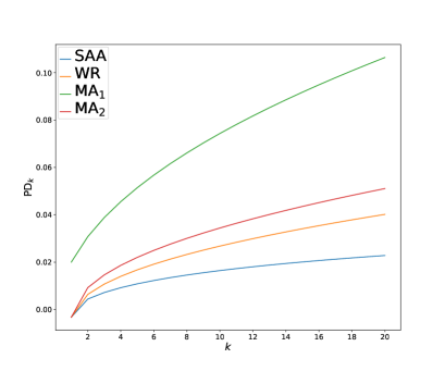
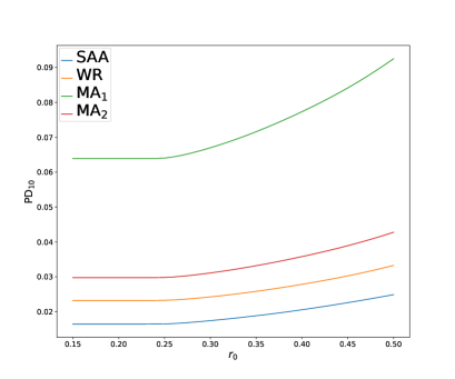
Figure EC.4: The optimized values of ${\rm PD}_{k}$ under mean-variance uncertainty. Left: $r_{0}=0.2$ and $k\in[1,20]$; Right: $k=10$ and $r_{0}\in[0.15,0.5]$.

Similarly to Section 8.2, we choose 350 trading days for the initial training, and compute the optimal portfolio weights in each day with a rolling window. Figure EC.5 presents the SAA approach, Markowitz model, and WR and MA approaches under Wasserstein uncertainty set with t benchmark distribution and mean-variance uncertainty over the remaining 300 trading days with $r_{0}=0.2$ and $k=2$ (left) or $k=20$ (right). In the case $k=2$, the WR and ${\rm MA}_{2}$ approaches exhibit comparable performance but underperform the other approaches. In the first 150 trading days, the SAA approach outperform the others, and its performance aligns closely with the ${\rm MA}_{1}$ approach thereafter, with the Markowitz model delivering the best performance. In the case $k=20$, the Markowitz model stands out with superior performance, particularly in the final 100 trading days. Both the MA and WR approaches perform very similarly, trailing slightly behind the SAA approach during the first 150 trading days.

Tables EC.1 and EC.2 present the Sharpe ratios and the nominal transaction cost, respectively, for SAA, Markowitz, WR and MA approaches under mean-variance uncertainty as well as Wasserstein uncertainty, which has been shown in Section 8.2. With $r_{0}=0.2$ and $0.3$, the MA and WR approaches based on Wasserstein uncertainty have smaller transaction costs than the other approaches. Additionally, these approaches also exhibit larger Sharpe ratios. The $\rm MA_{1}$ approach with mean-variance uncertainty has the smallest transaction cost for $r_{0}=0.1$.

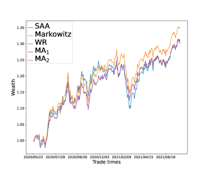
Figure EC.5: Wealth evolution for different portfolio strategies from May 2020 to Aug 2021 with $r_{0}=0.2$. Left: $k=2$; Right: $k=20$.

Table EC.1: Annualized return (AR), annualized volatility (AV) and Sharpe ratio (SR) for different portfolio strategies from May 2020 to Aug 2021 with $r_{0}=0.2$

	AR ($\%$)		AV ($\%$)		SR ($\%$)
Approach	$k=2$	$k=20$	$k=2$	$k=20$	$k=2$	$k=20$
SAA	25.42	26.72	14.82	14.35	170.4	185.0
Markowitz	29.50	29.50	13.54	13.54	216.6	216.6
W-WR	32.75	30.79	14.25	13.30	228.7	230.3
W-${\rm MA}_{2}$	33.77	32.01	14.48	13.56	232.0	234.9
MV-WR	22.10	25.60	15.30	12.86	143.4	197.8
MV-${\rm MA}_{1}$	25.26	25.93	12.92	12.81	194.2	201.1
MV-${\rm MA}_{2}$	22.24	25.71	13.90	12.84	158.8	198.9

Note: W-WR: WR with Wasserstein uncertainty; W-${\rm MA}_{2}$: ${\rm MA}_{2}$ with Wasserstein uncertainty; MV-WR: WR with mean-variance uncertainty; MV-${\rm MA}_{1}$: ${\rm MA}_{1}$ with mean-variance uncertainty; MV-${\rm MA}_{2}$: ${\rm MA}_{2}$ with mean-variance uncertainty.

Table EC.2: Nominal transaction cost $\sum_{t=1}^{T}\|\mathbf{w}_{t+1}-\mathbf{w}_{t}\|_{1}/T$ with $\varepsilon=0.01$ and $T=299$

	$r_{0}=0.1$		$r_{0}=0.2$		$r_{0}=0.3$
Approach	$k=2$	$k=20$	$k=2$	$k=20$	$k=2$	$k=20$
SAA	0.0549	0.0071	0.0871	0.0121	0.0969	0.0833
Markowitz	0.0102	0.0102	0.0110	0.0110	0.0746	0.0746
W-WR	0.0127	0.0032	0.0127	0.0033	0.0271	0.0382
W-${\rm MA}_{2}$	0.0114	0.0035	0.0105	0.0035	0.0239	0.0348
MV-WR	0.0321	0.0062	0.0766	0.0074	0.0690	0.0714
MV-${\rm MA}_{1}$	0.0080	0.0024	0.0108	0.0047	0.0714	0.0714
MV-${\rm MA}_{2}$	0.0236	0.0049	0.0496	0.0065	0.0714	0.0714

Remark EC.4.

The similar performance of MA and WR approaches for large $k$ is not a coincidence. In the setting of mean-variance uncertainty, as $k$ grows, the weights $\beta_{k}$, $\gamma_{k}$ and $\eta_{k}$ in the optimization problems (EC.30), (EC.31) and (EC.32) also grow. If these weights are large enough, then the terms involving $\sqrt{{\mathbf{w}}^{\top}\Sigma{\mathbf{w}}}$ in those problems become dominant in the optimization. For this reason, Problems (EC.30), (EC.31) and (EC.32) are similar to the case that the mixture of mean and standard variance as the objective risk measure with a large weight on the standard variance.

G.2 Wasserstein uncertainty with normal benchmark distribution

We follow the portfolio selection setting discussed in Section 8.2 under Wassserstein uncertainty with a fitted normal benchmark distribution. The considered optimization problems have the same form of (37) and (38) with the unit variance t-distribution replaced by the standard norm distribution. Figure EC.6 presents the robust risk values of the optimization problem with the SAA, WR and MA approaches for different values of $\varepsilon$, $r_{0}$ and $k$ using the whole-period data. In the left panel, we see that SSA may be the largest if $\varepsilon\leqslant 0.002$, because the empirical cdf of the data may be outside the Wasserstein uncertainty set if $\varepsilon$ is too small. As seen from Theorem 4, although the multivariate normal distribution of $\mathbf{X}$ leads to a light-tailed benchmark distribution of $\mathbf{w}^{\top}\mathbf{X}$, the robust model we use in the MA approach is heavy-tailed. Figure EC.7 reports the wealth process under SAA approach, and WR and MA approaches under Wasserstein uncertainty with a normal benchmark distribution as well as a t-benchmark distribution which has been shown in Section 8.2. All robust approaches perform similarly, and they generally outperform SAA approach, especially after the first 150 trading days.

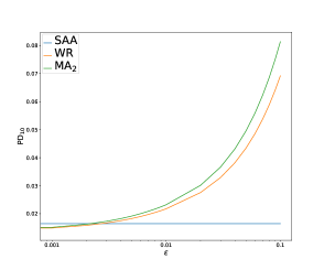
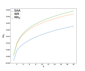
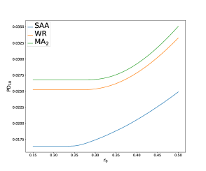
Figure EC.6: The optimized values of ${\rm PD}_{k}$ under Wasserstein uncertainty. Left: $r_{0}=0.2$, $k=10$ and $\varepsilon\in[0,0.1]$; Middle: $r_{0}=0.2$, $\varepsilon=0.01$ and $k\in[1,20]$; Right: $k=10$, $\varepsilon=0.01$ and $r_{0}\in[0.15,0.5]$.

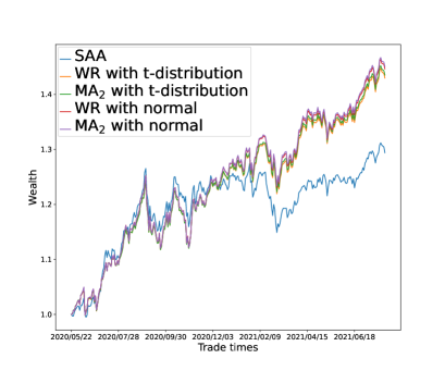
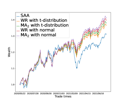
Figure EC.7: Wealth evolution for different portfolio strategies from May 2020 to Aug 2021 ($\varepsilon=0.01$, $r_{0}=0.2$). Left: $k=2$; Right: $k=20$.

Table EC.3: Summary statistics of daily returns of the 20 stocks, including sample mean ($\times 10^{-3}$), sample standard deviation (SD, $\times 10^{-4}$), and sample correlations

	Mean	SD	1	2	3	4	5	6	7	8	9	10	11	12	13	14	15	16	17	18	19	20
1	2.3	5.1	1
2	1.8	4.0	0.784	1
3	1.6	3.8	0.679	0.786	1
4	1.4	3.7	0.660	0.714	0.644	1
5	1.8	5.0	0.707	0.838	0.716	0.704	1
6	1.3	6.3	0.496	0.546	0.505	0.614	0.612	1
7	3.2	11.6	0.583	0.600	0.519	0.560	0.574	0.445	1
8	1.6	3.7	0.637	0.737	0.685	0.443	0.653	0.330	0.473	1
9	0.7	2.0	0.485	0.563	0.478	0.332	0.429	0.251	0.323	0.568	1
10	1.3	2.0	0.588	0.647	0.531	0.529	0.600	0.405	0.447	0.513	0.534	1
11	0.8	2.1	0.438	0.520	0.403	0.378	0.449	0.330	0.334	0.377	0.479	0.680	1
12	0.9	2.3	0.491	0.581	0.478	0.371	0.494	0.271	0.338	0.538	0.656	0.610	0.610	1
13	1.4	5.0	0.626	0.715	0.662	0.457	0.628	0.308	0.472	0.922	0.534	0.470	0.349	0.513	1
14	1.1	4.8	0.500	0.580	0.534	0.357	0.482	0.292	0.379	0.611	0.565	0.483	0.363	0.491	0.567	1
15	1.0	5.1	0.437	0.493	0.498	0.308	0.402	0.198	0.307	0.649	0.410	0.310	0.274	0.392	0.670	0.415	1
16	1.3	3.8	0.606	0.681	0.584	0.424	0.598	0.372	0.471	0.654	0.494	0.569	0.469	0.548	0.613	0.593	0.539	1
17	0.6	6.6	0.584	0.646	0.552	0.461	0.587	0.397	0.434	0.562	0.442	0.514	0.437	0.444	0.548	0.457	0.409	0.560	1
18	2.1	6.5	0.659	0.742	0.636	0.595	0.742	0.445	0.522	0.653	0.395	0.513	0.374	0.425	0.640	0.428	0.428	0.595	0.540	1
19	1.6	5.7	0.525	0.544	0.535	0.321	0.440	0.241	0.364	0.649	0.452	0.398	0.321	0.426	0.633	0.556	0.631	0.621	0.521	0.441	1
20	0.7	3.7	0.479	0.546	0.513	0.354	0.450	0.227	0.361	0.630	0.563	0.455	0.390	0.543	0.623	0.521	0522	0.595	0.555	0.391	0.630	1

References

- Ararat et al. (1999) Ararat, Ç., Hamel, A. H. and Rudloff, B. (2017). Set-valued shortfall and divergence risk measures. International Journal of Theoretical and Applied Finance, 20(5), 1750026.
- Artzner et al. (1999) Artzner, P., Delbaen, F., Eber, J.-M. and Heath, D. (1999). Coherent measures of risk. Mathematical Finance, 9(3), 203–228.
- BCBS (2019) BCBS (2019). Minimum Capital Requirements for Market Risk. February 2019. Basel Committee on Banking Supervision. Basel: Bank for International Settlements.
- Bellini et al. (2014) Bellini, F., Klar, B., Müller, A. and Rosazza Gianin, E. (2014). Generalized quantiles as risk measures. Insurance: Mathematics and Economics, 54(1), 41–48.
- Ben-Tal and Nemirovski (2001) Ben-Tal, A. and Nemirovski, A. (2001). Lectures on Modern Convex Optimization: Analysis, Algorithms, and Engineering Applications. SIAM, Philadelphia, USA.
- Blanchet et al. (2022) Blanchet, J., Chen, L. and Zhou, X. (2022). Distributionally robust mean-variance portfolio selection with Wasserstein distances. Management Science, 68(9), 6382–6410.
- Blanchet et al. (2019) Blanchet, J., Kang, Y. and Murthy, K. (2019). Robust Wasserstein profile inference and applications to machine learning. Journal of Applied Probability, 56(3), 830–857.
- Blanchet and Murthy (2019) Blanchet, J. and Murthy, K. (2019). Quantifying distributional model risk via optimal transport. Mathematics of Operations Research, 44(2), 565–600.
- Cerreia-Vioglio et al. (2021) Cerreia-Vioglio, S., Hansen, L. P., Maccheroni, F. and Marinacci, M. (2021). Making decisions under model misspecification. SSRN: 3666424.
- Chambers (2009) Chambers, C. P. (2009). An axiomatization of quantiles on the domain of distribution functions. Mathematical Finance, 19(2), 335–342.
- Chen et al. (2011) Chen, L., He, S. and Zhang, S. (2011). Tight bounds for some risk measures, with applications to robust portfolio selection. Operations Research, 59, 847–865.
- Cherny and Madan (2009) Cherny, A. S. and Madan, D. (2009). New measures for performance evaluation. Review of Financial Studies, 22(7), 2571–2606.
- Cambou and Filipović (2017) Cambou, M. and Filipović, D. (2017). Model uncertainty and scenario aggregation. Mathematical Finance, 27(2), 534–567.
- Cont et al. (2010) Cont, R., Deguest, R. and Scandolo, G. (2010). Robustness and sensitivity analysis of risk measurement procedures. Quantitative Finance. 10, 593–606.
- Cowell (2011) Cowell, F. A. (2011). Measuring Inequality. 3rd ed. Oxford: Oxford University Press.
- Delage et al. (2019) Delage, E., Kuhn, D. and Wiesemann, W. (2019). ”Dice”-sion-making under uncertainty: when can a random decision reduce risk? Management Science, 65(7), 3282–3301.
- Delage and Ye (2010) Delage, E. and Ye, Y. (2010). Distributionally robust optimization under moment uncertainty with application to data-driven problems. Operations research, 58(3), 595–612.
- Dentcheva (2023) Dentcheva, D. (2023). Relations between risk-averse models in extended two-stage stochastic optimization. Serdica Mathematical Journal, forthcoming.
- Dentcheva and Ruszczynski (2003) Dentcheva, D. and Ruszczyński, A. (2003). Optimization with stochastic dominance constraints. SIAM Journal on Optimization, 14(2), 548–566.
- Dentcheva and Ruszczynski (2004) Dentcheva, D. and Ruszczyński, A. (2004). Optimality and duality theory for stochastic optimization problems with nonlinear dominance constraints. Mathematical Programming, 99(2), 329–350.
- Embrechts and Puccetti (2006) Embrechts, P. and Puccetti, G. (2006). Bounds for functions of multivariate risks. Journal of Multivariate Analysis, 97(2), 526–547.
- Embrechts et al. (2013) Embrechts, P., Puccetti, G. and Rüschendorf, L. (2013). Model uncertainty and VaR aggregation. Journal of Banking and Finance, 37(8), 2750–2764.
- Embrechts et al. (2022) Embrechts, P., Schied, A. and Wang, R. (2022). Robustness in the optimization of risk measures. Operations Research, 70(1), 95–110.
- Embrechts et al. (2021) Embrechts, P., Mao, T., Wang, Q. and Wang, R. (2021). Bayes risk, elicitability, and the Expected Shortfall. Mathematical Finance, 31, 1190–1217.
- Esfahani and Kuhn (2018) Esfahani, P. M. and Kuhn, D. (2018). Data-driven distributionally robust optimization using the Wasserstein metric: Performance guarantees and tractable reformulations. Mathematical Programming, 171(1), 115–166.
- Föllmer and Schied (2016) Föllmer, H. and Schied, A. (2016). Stochastic Finance. An Introduction in Discrete Time. (Fourth Edition.) Walter de Gruyter, Berlin.
- Fu et al. (2022) Fu, M., Li, X. and Zhang, L., (2021) Data-driven feature-based newsvendor: A distributionally robust approach. SSRN: 3885663.
- Gao and Kleywegt (2016) Gao, R. and Kleywegt, A. J. (2016). Distributionally robust stochastic optimization with Wasserstein distance. arXiv preprint arXiv:1604.02199.
- Ghaoui et al. (2003) Ghaoui, L. M. E., Oks, M. and Oustry, F. (2003). Worst-case value-at-risk and robust portfolio optimization. Operations Research, 51, 543–556.
- Glasserman and Xu (2014) Glasserman, P. and Xu, X. (2014). Robust risk measurement and model risk. Quantitative Finance, 14(1), 29–58.
- Hamel and Heyde (2010) Hamel, A. H. and Heyde, F. (2010). Duality for set-valued measures of risk. SIAM Journal on Financial Mathematics, 1(1), 66–95.
- Hamel et al. (2011) Hamel, A. H., Heyde, F. and Rudloff, B. (2011). Set-valued risk measures for conical market models. Mathematics and Financial Economics, 5(1), 1–28.
- Han et al. (2023) Han, X., Wang, B., Wang, R. and Wu, Q. (2023). Risk concentration and the mean-Expected Shortfall criterion. Mathematical Finance, published online.
- Hansen and Sargent (2001) Hansen, L. P. and Sargent, T. J. (2001). Robust control and model uncertainty. American Economic Review. 91(2), 60–66.
- He and Peng (2018) He, X. and Peng, X. (2018). Surplus-invariant, law-invariant, and conic acceptance sets must be the sets induced by Value-at-Risk. Operations Research, 66(5), 1268–1276.
- Huang et al. (2020) Huang, R. J., Tzeng, L. Y. and Zhao, L. (2020). Fractional degree stochastic dominance. Management Science, 66(10), 4630–4647.
- Jagannathan (1977) Jagannathan, R. (1977). Minimax procedure for a class of linear programs under uncertainty. Operations Research, 25(1), 173–177.
- Kertz and Rösler (2000) Kertz, R. P. and Rösler, U. (2000). Complete lattices of probability measures with applications to martingale theory. IMS Lecture Notes Monograph Series, 35, 153-177.
- Klibanoff et al. (2005) Klibanoff, P., Marinacci, M. and Mukerji, S. (2005). A smooth model of decision making under uncertainty. Econometrica, 73(6), 1849–1892.
- Kou and Peng (2016) Kou, S. and Peng, X. (2016). On the measurement of economic tail risk. Operations Research, 64(5), 1056–1072.
- Kupper and Zapata (2021) Kupper, M. and Zapata, J. M. (2021). Large deviations built on max-stability. Bernoulli, 27(2), 1001–1027.
- Kusuoka (2001) Kusuoka, S. (2001). On law invariant coherent risk measures. Advances in Mathematical Economics. 3, 83–95.
- Li et al. (2018) Li, L., Shao, H., Wang, R. and Yang, J. (2018). Worst-case range value-at-risk with partial information. SIAM Journal on Financial Mathematics. 9(1), 190–218.
- Li (2018) Li, Y. M. J. (2018). Technical note: closed-form solutions for worst-case law invariant risk measures with application to robust portfolio optimization. Operations Research, 66(6), 1533–1541.
- Liu et al. (2022) Liu, F., Mao, T., Wang, R. and Wei, L. (2022). Inf-convolution, optimal allocations, and model uncertainty for tail risk measures. Mathematics of Operations Research, forthcoming.
- Liu and Wang (2021) Liu, F. and Wang, R. (2021). A theory for measures of tail risk. Mathematics of Operations Research, 46(3), 1109–1128.
- Lo (1987) Lo, A. (1987). Semiparametric upper bounds for option prices and expected payoffs. Journal of Financial Economics, 19(2), 373–388.
- Markowitz (1952) Markowitz, H. (1952). Portfolio selection, Journal of Finance, 7(1), 77–91.
- Maccheroni et al. (2006) Maccheroni, F., Marinacci, M. and Rustichini, A. (2006). Ambiguity aversion, robustness, and the variational representation of preferences. Econometrica, 74(6), 1447–1498.
- McNeil et al. (2015) McNeil, A. J., Frey, R. and Embrechts, P. (2015). Quantitative Risk Management: Concepts, Techniques and Tools. (Revised Edition.) Princeton University Press, Princeton, NJ.
- Müller et al. (2017) Müller, A., Scarsini, M., Tsetlin, I. and Winkler. R. L. (2017). Between first and second-order stochastic dominance. Management Science, 63(9), 2933–2947.
- Müller and Scarsini (2006) Müller, A. and Scarsini, M. (2006). Stochastic order relations and lattices of probability measures. SIAM Journal on Optimization. 16(4), 1024–1043.
- Müller and Stoyan (2002) Müller, A. and Stoyan, D. (2002). Comparison Methods for Stochastic Models and Risks. John Wiley & Sons, Hoboken.
- Natarajan et al. (2008) Natarajan, K., Pachamanova, D. and Sim, M. (2008). Incorporating asymmetric distributional information in robust value-at-risk optimization. Management Science, 54(3), 573–585.
- Natarajan et al. (2010) Natarajan, K., Sim, M. and Uichanco, J. (2010). Tractable robust expected utility and risk models for portfolio optimization. Mathematical Finance, 20, 695–731.
- Newey and Powell (1987) Newey, W. K., Powell, J. L. (1987). Asymmetric least squares estimation and testing. Econometrica, 55(4), 819–847.
- Olivares-Nadal and DeMiguel (2018) Olivares-Nadal, A. V. and DeMiguel, V. (2018). A robust perspective on transaction costs in portfolio optimization. Operations Research, 66(3), 733–739.
- Popescu (2007) Popescu, I. (2007). Robust mean-covariance solutions for stochastic optimization. Operations Research, 55(1), 98–112.
- Postek et al. (2016) Postek, K., den Hertog, D. and Melenberg, B. (2016). Computationally tractable counterparts of distributionally robust constraints on risk measures. SIAM Review, 58(4), 603–650.
- Rockafellar and Uryasev (2002) Rockafellar, R.T. and Uryasev, S. (2002). Conditional value-at-risk for general loss distributions. Journal of Banking and Finance, 26(7), 1443–1471.
- Rothschild and Stiglitz (1970) Rothschild, M. and Stiglitz, J. (1970). Increasing risk I. A definition. Journal of Economic Theory, 2(3), 225–243.
- Ruszczyński and Shapiro (2006) Ruszczyński, A. and Shapiro, A. (2006). Optimization of convex risk functions. Mathematics of Operations Research, 31(3), 433–452.
- Shaked and Shanthikumar (2007) Shaked, M. and Shanthikumar, J. G. (2007). Stochastic Orders. Springer Series in Statistics.
- Shapiro (2013) Shapiro, A. (2013). On Kusuoka representation of law invariant risk measures. Mathematics of Operations Research, 38(1), 142-152.
- Shapiro et al. (2021) Shapiro, A., Dentcheva, D. and Ruszczynski, A. (2021). Lectures on stochastic programming: modeling and theory. Society for Industrial and Applied Mathematics.
- Schmeidler (1989) Schmeidler, D. (1989). Subjective probability and expected utility without additivity. Econometrica, 57(3), 571–587.
- Wang (1995) Wang, S. (1995). Insurance pricing and increased limits ratemaking by proportional hazards transforms. Insurance: Mathematics and Economics, 17(1), 43–54.
- Wang et al. (2013) Wang, R., Peng, L. and Yang, J. (2013). Bounds for the sum of dependent risks and worst Value-at-Risk with monotone marginal densities. Finance and Stochastics, 17(2), 395–417.
- Wang et al. (2020) Wang, R., Wei, Y. and Willmot, G. E. (2020). Characterization, robustness and aggregation of signed Choquet integrals. Mathematics of Operations Research, 45(3), 993–1015.
- Wang and Ziegel (2021) Wang, R. and Ziegel, J. F. (2021). Scenario-based risk evaluation. Finance and Stochastics, 25, 725–756.
- Wang and Zitikis (2021) Wang, R. and Zitikis, R. (2021). An axiomatic foundation for the Expected Shortfall. Management Science, 67, 1413–1429.
- Wiesemann et al. (2014) Wiesemann, W., Kuhn, D. and Sim, M. (2014). Distributionally robust convex optimization. Operations Research, 62(6), 1203–1466.
- Wozabal (2014) Wozabal, D. (2014). Robustifying convex risk measures for linear portfolios: A nonparametric approach. Operations Research, 62(6), 1302–1315.
- Yaari (1987) Yaari, M. E. (1987). The dual theory of choice under risk. Econometrica, 55(1), 95–115.
- Zhu and Fukushima (2009) Zhu, M. S. and Fukushima, M. (2009). Worst-case conditional value-at-risk with application to robust portfolio management. Operations Research, 57(5), 1155–1168.
Online Supplement: Technical Appendices

References

- Bäuerle and Müller (2006) Bäuerle, N. and Müller, A. (2006). Stochastic orders and risk measures: consistency and bounds. Insurance: Mathematics and Economics, 38(1), 132–148.
- Berti et al. (2007) Berti, P., Pratelli, L. and Rigo, P. (2007). Skorohod representation on a given probability space. Probability Theory and Related Fields, 137(3-4), 277–288.
- Cerreia-Vioglio et al. (2011) Cerreia-Vioglio, S., Maccheroni, F., Marinacci, M. and Montrucchio, L. (2011). Risk measures: rationality and diversification. Mathematical Finance, 21(4), 743–774.
- Davey and Priestley (2002) Davey, B. A. and Priestley, H. A. (2002). Introduction to Lattices and Order, Cambridge University Press, New York.
- Föllmer and Schied (2016) Föllmer, H. and Schied, A. (2016). Stochastic Finance. An Introduction in Discrete Time. (Fourth Edition.) Walter de Gruyter, Berlin.
- Jia et al. (2020) Jia, G., Xia, J. and Zhao, R. (2020). Monetary risk measures. arXiv: 2012.06751.
- Kaina and Rüschendorf (2009) Kaina, M. and Rüschendorf, L. (2009). On convex risk measures on -spaces. Mathematical Methods of Operations Research, 69(3), 475–495.
- Kertz and Rösler (2000) Kertz, R. P. and Rösler, U. (2000). Complete lattices of probability measures with applications to martingale theory. IMS Lecture Notes Monograph Series, 35, 153-177.
- Rockafellar (1970) Rockafellar, R. (1970). Convex analysis, Princeton landmarks in mathematics and physics, Princeton University Press.
- Liu et al. (2022) Liu, F., Mao, T., Wang, R. and Wei, L. (2022). Inf-convolution, optimal allocations, and model uncertainty for tail risk measures. Mathematics of Operations Research, 47(3), 2494–2519.
- Shorrocks (1983) Shorrocks, A. F. (1983). Ranking income distributions. Economica, 50, 3–17.
- Zhu and Fukushima (2009) Zhu, M. S. and Fukushima, M. (2009). Worst-case conditional value-at-risk with application to robust portfolio management. Operations Research, 57(5), 1155–1168.