Can molecular simulations reliably compare homogeneous and heterogeneous ice nucleation?

Abstract

In principle, the answer to the posed titular question is undoubtedly ‘yes.’ But in practice, requisite reference data for homogeneous systems have been obtained with a treatment of intermolecular interactions that is different from that typically employed for heterogeneous systems. In this article, we assess the impact of the choice of truncation scheme when comparing water in homogeneous and inhomogeneous environments. Specifically, we use explicit free energy calculations and a simple mean field analysis to demonstrate that using the ‘cut-and-shift’ version of the Lennard-Jones potential (common to most simple point charge models of water) results in a systematic increase in the melting temperature of ice I_h. In addition, by drawing an analogy between a change in cutoff and a change in pressure, we use existing literature data for homogeneous ice nucleation at negative pressures to suggest that enhancements due to heterogeneous nucleation may have been overestimated by several orders of magnitude.

I Introduction

The formation of ice is a process of great importance across a broad range of fields, from climate science Tan, Storelvmo, and Zelinka (2016); Slater et al. (2016) to biology Bar Dolev, Braslavsky, and Davies (2016). Obtaining a detailed molecular-level understanding of both homogeneous nucleation (i.e., in the absence of foreign bodies such as mineral particles) and heterogeneous nucleation (i.e., in the presence of surfaces due to foreign bodies) has attracted major research efforts from both experimental and simulation groups Murray et al. (2012); Sosso et al. (2016a). With regard to the latter, in a bid to reduce computational cost, most molecular simulations employ empirical potentials that approximately describe the interactions between water molecules. While many types of empirical potentials exist Molinero and Moore (2009); Vega and Abascal (2011); Cisneros et al. (2016), simple point charge (SPC) models are one of the most commonly used. Note that we use ‘SPC model’ to refer to the general class of water model detailed in Sec. I.1 rather than the specific water model of Ref. H. J. C. Berendsen and Hermans, 1981. In addition to being relatively simple and computationally efficient, an appealing feature of SPC models is that they preserve the donor-acceptor nature of water’s hydrogen-bond network, which can be especially important for heterogeneous nucleation, e.g., in the presence of kaolinite Cox et al. (2013); Sosso et al. (2016b).

To ensure short-ranged repulsion between molecules, most commonly used SPC water models, at least formally, employ the Lennard-Jones (LJ) potential Lennard-Jones (1931),

$$u^{(\infty)}_{\rm LJ}(r)=4\varepsilon\Bigg{[}\bigg{(}\frac{\sigma}{r}\bigg{)}^{12}-\bigg{(}\frac{\sigma}{r}\bigg{)}^{6}\Bigg{]},$$ (1)

which is parameterized by an energy scale $\varepsilon$ and length scale $\sigma$, and where $r$ indicates the distance between two water molecules (usually the separation between their oxygen atoms). Figure 1a shows $u^{(\infty)}_{\rm LJ}$.

In addition to explicit electrostatic interactions between water molecules, the $-(\sigma/r)^{6}$ term contributes to the cohesive energy of the system. Despite being the basis for most SPC water models, however, $u^{(\infty)}_{\rm LJ}$ is rarely sampled explicitly; due to the infinite range of the attractive $-(\sigma/r)^{6}$ term, it is common to truncate $u^{(\infty)}_{\rm LJ}$ in some fashion (see, e.g., Refs. Frenkel and Smit, 2002; Allen and Tildesley, 2017). Two common procedures, which we detail in Sec. I.1, are to use ‘tail corrections’ or to ‘cut-and-shift’, as shown in Figs. 1a and 1b, respectively. By comparing these plots it can be seen that, while similar, these two truncation procedures result in different intermolecular potentials, and will in general have different properties. For example, thermodynamic properties such as interfacial tension and the location of phase boundaries are known to be affected Smit (1992); Johnson, Zollweg, and Gubbins (1993); Baidakov, Chernykh, and Protsenko (2000); Hafskjold et al. (2019); Ghoufi, Malfreyt, and Tildesley (2016); Fitzner et al. (2017).

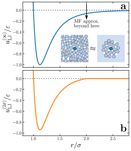
Figure 1: The two variations of the LJ potential studied in this article. (a) The solid blue curve shows $u_{\rm LJ}^{(\infty)}$ given by Eq. 1. For homogeneous systems $u^{(\infty)}_{\rm LJ}$ is well-approximated by truncating interactions at a given cutoff (indicated by the arrow), and applying ‘tail corrections’ to account for neglected interactions; this is equivalent to a mean field approximation. Inset: schematic representation of the tail correction procedure. The blue shaded region indicates that interactions between the tagged particle (dark blue) and those beyond the cutoff radius are accounted for in an average sense. (b) The ‘cut-and-shift’ variant of the LJ potential (see Eq. 7) has vanishing interactions beyond the cutoff. It is a different potential with different properties compared to $u_{\rm LJ}^{(\infty)}$. In both examples, the cutoff radius is $2\sigma$.

Why then, would another article that investigates the effects of truncating the LJ potential be useful? Put simply, the phase behavior of SPC water models has been studied extensively using the tail corrected truncation scheme Sanz et al. (2004); Vega, Sanz, and Abascal (2005); Abascal and Vega (2005); Abascal et al. (2005). And the same can be said for most calculations of homogeneous ice nucleation rates Espinosa et al. (2014); Haji-Akbari and Debenedetti (2015); Espinosa et al. (2016); Bianco et al. (2021). Yet, as we will discuss in more detail below, the use of tail corrections makes direct comparison to inhomogeneous systems challenging. While a simple approach to mitigate discrepancies between homogeneous and inhomogeneous systems would be consistent use of cut-and-shift potentials, it is unreasonable to expect that each study of heterogeneous nucleation is accompanied by: (i) a full recalculation of the melting temperature or phase diagram; and (ii) recomputation of the homogeneous nucleation rate. [To give a sense of perspective, in Ref. Haji-Akbari and Debenedetti, 2015 over $21\times 10^{6}$ CPU hours were required to compute the homogeneous nucleation rate with forward flux sampling (FFS).] In this article, we address the first issue directly, by outlining a procedure to approximately predict the change in melting temperature between the tail-corrected and cut-and-shift systems. We then combine our results with those in Ref. Bianco et al., 2021 to estimate the impact on the comparison of homogeneous and heterogeneous nucleation rates.

I.1 Formulating the problem

We now detail the tail-correction and cut-and-shift truncation schemes, as well as illustrate the inconsistencies that appear between homogeneous and inhomogeneous systems. We are concerned with SPC water models that formally have a potential energy function of the kind

$$U^{(\infty)}(\mathbf{R}^{N})=\sum_{i<j}^{N}u^{(\infty)}_{\rm LJ}(|\mathbf{r}^{\rm(O)}_{ij}|)+\sum_{i<j}^{N}\sum_{\alpha,\beta}\frac{q^{(\alpha)}q^{(\beta)}}{|\mathbf{r}^{(\alpha)}_{j}-\mathbf{r}^{(\beta)}_{i}|},$$ (2)

where $\mathbf{R}^{N}$ denotes the set of atomic positions for a configuration of $N$ water molecules, $\mathbf{r}_{ij}^{\rm(O)}$ is the separation vector between the oxygen atoms of molecules $i$ and $j$, and $q^{(\alpha)}_{i}$ is the charge of site $\alpha$, located at $\mathbf{r}_{i}^{(\alpha)}$, of molecule $i$. (We adopt a unit system in which $4\pi\epsilon_{0}=1$, where $\epsilon_{0}$ is the permittivity of free space.) The second set of sums in Eq. 2, which we will denote $U_{\rm elec}$ hereafter, describes electrostatic interactions between molecules, while the first set of sums involve the LJ potential. For SPC models of water, the choice of $u^{(\infty)}_{\rm LJ}$ is rooted in grounds of convention and convenience, rather than having any deep theoretical justification. Nonetheless, SPC models of the kind formally described by Eq. 2 have been, are, and will likely continue (at least in the near future) to be the foundation for many molecular simulations of water’s condensed phases.

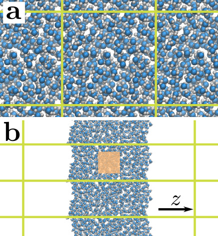
Figure 2: Typical simulation geometries for water. (a) Homogeneous bulk water simulated under 3D bulk periodic boundary conditions such that the average density is independent of position, $\langle\rho(\mathbf{r})\rangle=\bar{\rho}(p)$. (b) The slab geometry employed to study interfacial systems also employs periodic boundary conditions (often in 3D) and has a density profile that varies with position $z$ along the surface normal, such that in general $\langle\rho(z)\rangle\neq\bar{\rho}$. For thick enough slabs, regions far removed from the interfaces (as indicated, e.g., by the orange box)) have an average density equal to $\bar{\rho}(p=0)$ for the homogeneous system. Green lines indicate the boundaries of the periodically repeated simulation cells.

So far, we have referred to SPC models of water that are ‘formally’ described by the potential energy given by Eq. 2. But as already mentioned, in practice $u^{(\infty)}_{\rm LJ}$ is usually truncated in some fashion Frenkel and Smit (2002); Allen and Tildesley (2017). For the tail-correction scheme, one employs a simple truncation,

$$u_{\rm LJ}^{(r_{\rm c}\to\infty)}(r)=\begin{cases}u^{(\infty)}_{\rm LJ}(r),&r\leq r_{\rm c},\\ 0,&r>r_{\rm c},\end{cases}$$ (3)

and then approximately accounts for the effects of truncation by adding a mean field (MF) correction,

$$\frac{\Delta_{\rm MF}U(r_{\rm c})}{N}=\frac{8\pi\epsilon\bar{\rho}\sigma^{3}}{9}\Bigg{[}\bigg{(}\frac{\sigma}{r_{\rm c}}\bigg{)}^{9}-3\bigg{(}\frac{\sigma}{r_{\rm c}}\bigg{)}^{3}\Bigg{]},$$ (4)

to the total potential energy:

$$U^{(\infty)}(\mathbf{R}^{N})\approx U^{(r_{\rm c}\to\infty)}(\mathbf{R}^{N})$$

$$=\sum_{i<j}^{N}u^{(r_{\rm c}\to\infty)}_{\rm LJ}(|\mathbf{r}^{\rm(O)}_{ij}|)+\Delta_{\rm MF}U(r_{\rm c})+U_{\rm elec}(\mathbf{R}^{N}),$$ (5)

where $\bar{\rho}$ is the average number density. The superscript ‘$(r_{\rm c}\to\infty)$’ indicates that, when used in combination with $\Delta_{\rm MF}U(r_{\rm c})$, a system that employs $u_{\rm LJ}^{(r_{\rm c}\to\infty)}$ satisfies $U^{(r_{\rm c}\to\infty)}\approx U^{(\infty)}$; this is reasonable provided that $g_{\rm OO}(r\geq r_{\rm c})\approx 1$, where $g_{\rm OO}$ is the oxygen-oxygen pair correlation function. In a similar spirit, the pressure can also be corrected in a MF fashion,

$$\Delta_{\rm MF}p(r_{\rm c})=\frac{32\pi\epsilon\bar{\rho}^{2}\sigma^{3}}{9}\Bigg{[}\bigg{(}\frac{\sigma}{r_{\rm c}}\bigg{)}^{9}-\frac{3}{2}\bigg{(}\frac{\sigma}{r_{\rm c}}\bigg{)}^{3}\Bigg{]}.$$ (6)

A comment is in order concerning the functional form of $u_{\rm LJ}^{(r_{\rm c}\to\infty)}$ (Eq. 3). The discontinuity at $r_{\rm c}$ suggests the presence of impulsive forces. Impulsive forces, however, are challenging to implement in molecular dynamics simulations, and it is standard practice to neglect them entirely. Moreover, as interactions beyond $r_{\rm c}$ are not neglected in $U^{(r_{\rm c}\to\infty)}$, but instead accounted for in a mean field fashion, we argue (see SM) that this neglect of impulsive forces is in fact consistent with the use of $\Delta_{\rm MF}U$ and $\Delta_{\rm MF}p$, as it accounts for a pointwise cancellation of impulsive forces.

The alternative cut-and-shift truncation scheme is:

$$u_{\rm LJ}^{(r_{\rm c})}(r)=\begin{cases}u^{(\infty)}_{\rm LJ}(r)-u^{(\infty)}_{\rm LJ}(r_{\rm c}),&r\leq r_{\rm c},\\ 0,&r>r_{\rm c},\end{cases}$$ (7)

such that the total potential energy is

$$U^{(r_{\rm c})}(\mathbf{R}^{N})=\sum_{i<j}^{N}u^{(r_{\rm c})}_{\rm LJ}(|\mathbf{r}^{\rm(O)}_{ij}|)+U_{\rm elec}(\mathbf{R}^{N}).$$ (8)

We will use the superscript ‘$(r_{\rm c})$’ to indicate that $u_{\rm LJ}^{(r_{\rm c})}$ is used. (We will, on occasion, drop the superscript notation, either because it is clear from context which truncation scheme is relevant, or because it is unimportant to differentiate between truncation schemes. When a numerical value of $r_{\rm c}$ is specified, it will be given in Ångstrom, though we will omit units from the superscript.) For simulations of systems in the canonical ($NVT$) ensemble, dynamics are unaffected by the choice of $U^{(r_{\rm c})}$ vs. $U^{(r_{\rm c}\to\infty)}$. The pressure, however, is sensitive to the choice of truncation scheme:

$$p^{(r_{\rm c}\to\infty)}\approx p^{(r_{\rm c})}+\Delta_{\rm MF}p(r_{\rm c}).$$ (9)

The implication of Eq. 9 is that dynamics in the isothermal-isobaric ($NpT$) ensemble are affected by the choice of $U^{(r_{\rm c})}$ vs. $U^{(r_{\rm c}\to\infty)}$. Furthermore, systems employing $U^{(r_{\rm c}\to\infty)}$ and $U^{(r_{\rm c})}$ will have, for the same $r_{\rm c}$, different equations of state Smit (1992); Johnson, Zollweg, and Gubbins (1993).

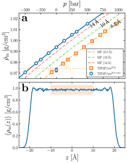
Figure 3: Evaluating the impact of $r_{\rm c}$ on $\bar{\rho}_{\rm m}$ for liquid TIP4P/ice at 300 K. (a) $\bar{\rho}_{\rm m}(p)$ for a homogeneous system. White-filled circles show results from constant-$p$ simulations of TIP4P/ice^(8.5→∞), and the solid blue line indicates a quadratic fit. Dashed lines indicate MF predictions (Eq. 9, see also Sec. III) for different $r_{\rm c}$, as indicated in the legend (the lines are also labeled). Orange squares show results from constant-$p$ simulations of TIP4P/ice^(8.5). The dotted line indicates $\bar{\rho}_{\rm m}(p=0)$ for TIP4P/ice^(8.5), which intercepts the TIP4P/ice^(8.5→∞) results at $p\approx-427$ bar. (b) $\langle\rho_{\rm m}(z)\rangle$ for a film of TIP4P/ice^(8.5→∞) in contact with its vapor (only part of the simulation cell is shown). Spatially averaging $\langle\rho_{\rm m}(z)\rangle$ in the slab’s interior, as indicated by the shaded region, gives an estimate for $\bar{\rho}_{\rm m}(0)$, which is plotted with the orange-filled circle in (a).

Implicit in our above discussion of MF corrections is that the system is homogeneous, such that the average equilibrium density $\langle\rho(\mathbf{r})\rangle=\bar{\rho}$ does not depend upon the position $\mathbf{r}$ in the fluid, as shown in Fig. 2a. If the system of interest is inhomogeneous, such as liquid water in coexistence with its vapor, a typical simulation approach is to employ the $NVT$ ensemble with a cuboidal cell that has an elongated dimension along the average surface normal; such a scenario is depicted in Fig. 2b. As $\Delta_{\rm MF}U$ and $\Delta_{\rm MF}p$ do not affect dynamics in the $NVT$ ensemble, effects of using $U^{(r_{\rm c}\to\infty)}$ for inhomogeneous systems would perhaps seem benign, resulting simply in a shift of the energy, i.e., $U^{(r_{\rm c}\to\infty)}(\mathbf{R}^{N})-U^{(\infty)}(\mathbf{R}^{N})=\text{const.}$

Potential problems arise, however, concerning thermodynamic consistency between the homogeneous and inhomogeneous systems. This is demonstrated in Fig. 3 for TIP4P/iceAbascal et al. (2005)—a commonly used SPC water model for studying ice formation—at 300 K, with $r_{\rm c}=8.5$ Å. Fig. 3a shows the average mass density $\bar{\rho}_{\rm m}(p)$ obtained from simulations of the homogeneous fluid employing either TIP4P/ice^(8.5→∞) or TIP4P/ice^(8.5). Fig. 3b shows the equilibrium mass density profile $\langle\rho_{\rm m}(z)\rangle$ for a film of TIP4P/ice^(8.5→∞) water approximately 40 Å thick, with its liquid/vapor interface spanning the $xy$ plane. Owing to the low vapor pressure of water, $p\approx 0$ in the vapor phase. As the normal component of the pressure tensor is independent of $z$ for a planar interface, and furthermore isotropic for $z$ in a bulk-like fluid region, it immediately follows that $p\approx 0$ deep in the slab’s interior Rowlinson and Widom (2002). Thermodynamic consistency then requires that

$$\frac{1}{\ell_{\rm bulk}}\int_{\ell_{\rm bulk}}\!\mathrm{d}z\,\langle\rho_{\rm m}(z)\rangle=\bar{\rho}_{\rm m}(p=0)$$

for TIP4P/ice^(8.5→∞), where $\ell_{\rm bulk}$ is a length over which $\langle\rho_{\rm m}(z)\rangle$ is bulk-like, as indicated, e.g., by the orange rectangles in Figs. 2b and 3b. The result of such an averaging procedure is indicated by the orange-filled circle in Fig. 3a; it is clearly inconsistent with $\bar{\rho}_{\rm m}(p=0)$ obtained from the homogeneous TIP4P/ice^(8.5→∞) simulation. As dynamics in the $NVT$ ensemble are unaffected by the choice of $U^{(r_{\rm c})}$ vs. $U^{(r_{\rm c}\to\infty)}$ we might expect, and indeed observe, that the result is instead consistent with $\bar{\rho}_{\rm m}(p=0)$ for TIP4P/ice^(8.5).

While schemes for effectively sampling $U^{(\infty)}$ do exist for heterogeneous systems (e.g., one can treat the attractive $-(\sigma/r)^{6}$ term in a Ewald fashionin’t Veld, Ismail, and Grest (2007); Alejandre and Chapela (2010); López-Lemus and Alejandre (2002, 2003), or use mean-field corrections that take the heterogeneous nature of the system into accountMíguez, Piñeiro, and Blas (2013); Janeček (2006); Salomons and Mareschal (1991); Guo, Peng, and Lu (1997); Guo and Lu (1997); de Gregorio et al. (2012)) their use is relatively limited compared to that of SPC water models. And, as discussed in Sec. I, no discrepancies would be observed with consistent use of $U^{(r_{\rm c})}$ for both the homogeneous and inhomogeneous systems, but information concerning phase behavior and homogeneous nucleation rates relevant to $U^{(r_{\rm c})}$ systems is scarce. In Sec. II, we therefore assess the effect of using $U^{(r_{\rm c})}$ instead of $U^{(r_{\rm c}\to\infty)}$ on the melting temperature $T_{\rm m}$ of ice I_h for SPC models of water. In particular we focus on TIP4P/ice Abascal et al. (2005) and TIP4P/2005 Abascal and Vega (2005), as these are most commonly used in simulations of ice nucleation. We stress, however, that the findings presented in this work readily extend to any SPC water model of the kind formally described by Eq. 2. To illustrate our findings, we will focus exclusively on results for TIP4P/ice in the main article, with results for TIP4P/2005 instead given in the Supplementary Material (SM). In Sec. IV we then estimate the impact of our findings on the comparison of homogeneous and heterogeneous ice nucleation rates.

As an aside, before proceeding to discuss our main results, we mention that our initial motivation for this study stemmed from recent work by Wang et al.Wang et al. (2020), who developed a new potential that gives broadly similar behavior to the LJ potential, but does not suffer, by construction, from ambiguities arising from the choice of truncation scheme. While our preliminary investigations suggested that the approach of Wang et al. could be used to develop workable SPC models of water, we judged their performance insufficiently strong to warrant introducing another set of SPC water models to the community. We therefore adopt a more pragmatic approach in this article by instead providing results and insights relevant to existing SPC water models that are heavily used by practitioners of molecular simulations.

II The melting point of ice I_h from free energy calculations

The central quantity under investigation in this study is the melting point of ice I_h under conditions of vanishing pressure, $p=0$ bar. To obtain estimates of $T_{\rm m}$ for TIP4P/ice${}^{(r_{\rm c})}$ and TIP4P/2005${}^{(r_{\rm c})}$, we need to establish the chemical potential at $p=0$ bar for both the ice [$\mu_{\rm ice}(T)$] and liquid [$\mu_{\rm liq}(T)$] phases: the point of intersection is $T_{\rm m}$. To compute $\mu_{\rm ice}$, we will adopt the Frenkel-Ladd approach Frenkel and Ladd (1984), adapted by Vega and co-workers for rigid SPC water models Noya, Conde, and Vega (2008); Vega et al. (2008); Aragones et al. (2013). As this approach has been detailed elsewhere, we present a detailed overview of our workflow in the SM, and discuss only the most salient aspects of the methodology in the main article.

First, we equilibrate a crystal of ice I_h comprising 768 molecules at a temperature $T_{\rm i}$ to obtain the average cell parameters. The cell parameters are then fixed to their average values, and the structure ‘minimized’ by a low temperature simulation at 0.1 K. (We adopt this approach as the standard minimizers in LAMMPS Plimpton (1995) are incompatible with the RATTLE algorithm Andersen (1983) used to impose the rigid body constraints of the water molecules.) Our reference structure is then this minimized crystal structure with no intermolecular interactions, and with the oxygen and hydrogen atoms of each water molecule tethered to their positions by a harmonic potential with spring constants $k_{\rm O}$ and $k_{\rm H}$, respectively. The difference in Helmholtz free energy (per molecule) $\Delta_{\rm r2i}a$ between this reference system and the interacting ice crystal of interest is then calculated by thermodyamic integration Kirkwood (1935), at temperature $T_{\rm i}$. The rigid body constraints, however, mean that we do not know the free energy of the reference system. We therefore define a ‘sub-reference’ system (with free energy $a_{\rm sub}$ that is calculated analytically) in which only the oxygen atoms of the water molecules are tethered, and compute the Helmholtz free energy between the sub-reference and reference systems $\Delta_{\rm s2r}a$, also by thermodynamic integration. The free energy of the ice crystal is then

$$a_{\rm ice}=a_{\rm kin}+a_{\rm sub}+\Delta_{\rm s2r}a+\Delta_{\rm r2i}a-k_{\rm B}T_{\rm i}\ln\frac{3}{2}-k_{\rm B}T_{\rm i}\ln 2,$$ (10)

with $a_{\rm kin}=3k_{\rm B}T_{\rm i}\ln(T_{0}/T_{\rm i})$, where $T_{0}$ is a reference temperature (see SM). We use $T_{0}=272$ K throughout this article. The final two terms respectively account for the Pauling entropy arising from proton disorder in ice I_h, and the fact that the reference system does not respect the permutational invariance of the two protons in a water molecule Aragones et al. (2013). The chemical potential is, in general, obtained from $\beta\mu_{\rm ice}=\beta a_{\rm ice}+\beta p/\bar{\rho}$; as $p=0$ bar, we simply have $\beta\mu_{\rm ice}=\beta a_{\rm ice}$. ($\beta=1/k_{\rm B}T$, where $k_{\rm B}$ is Boltzmann’s constant.) We note that there have been extensive studies to understand the effects of finite system size on the calculation of free energies for solids (see Ref. Vega et al., 2008 for a detailed discussion). Previous simulation studies suggest that the system size we use (768 molecules) is large enough to obtain a reliable estimate of $T_{\rm m}$ for ice I_hReinhardt and Cheng (2021). Moreover, it is likely that any finite size effects will largely cancel when comparing the two truncation schemes considered in this study.

For the liquid, we equilibrate a system comprising 360 molecules at $T_{\rm i}$ to obtain an estimate of $\bar{\rho}$. At this density, we then calculate the change in free energy $\Delta_{\rm LJ2w}a$ between the LJ fluid and the SPC water model under investigation using thermodynamic integration. For systems that employ $U^{(r_{\rm c}\to\infty)}$, we determine the excess free energy of the LJ fluid $a^{(r_{\rm c}\to\infty)}_{\rm LJ,ex}\approx a^{(\infty)}_{\rm LJ,ex}$ from the equation of state. (For consistency with previous calculations of water’s phase diagram Vega et al. (2008), we use the equation of state of Johnson et al.Johnson, Zollweg, and Gubbins (1993)) For systems using $U^{(r_{\rm c})}$, we must also compute the free energy difference $\Delta_{\rm tc2cs}a$ between the $U^{(r_{\rm c}\to\infty)}$ and $U^{(r_{\rm c})}$ systems. The free energy of the liquid is then

$$a_{\rm liq}^{(r_{\rm c})}=a_{\rm id}+a^{(r_{\rm c}\to\infty)}_{\rm LJ,ex}+\Delta_{\rm tc2cs}a+\Delta_{\rm LJ2w}a,$$ (11)

where $a_{\rm id}=k_{\rm B}T_{\rm i}\ln\big{(}\bar{\rho}(T_{0}/T_{\rm i})^{3}\big{)}-k_{\rm B}T_{\rm i}$ (see SM). An analogous expression holds for $a_{\rm liq}^{(r_{\rm c}\to\infty)}$, except that $\Delta_{\rm tc2cs}a$ is omitted. The chemical potential is simply $\beta\mu_{\rm liq}=\beta a_{\rm liq}$.

Once the chemical potential has been established at $T_{\rm i}$, we establish its temperature dependence by integrating the Gibbs-Helmholtz equation,

$$\beta\mu_{\rm ice}(T)=\beta_{\rm i}\mu_{\rm ice}(T_{\rm i})-\int_{T_{\rm i}}^{T}\!\mathrm{d}t\,\frac{h_{\rm ice}(t)}{k_{\rm B}t^{2}},$$ (12)

where $h_{\rm ice}$ is the enthalpy per molecule of ice, and $\beta_{\rm i}=1/k_{\rm B}T_{\rm i}$. An analogous expression holds for $\beta\mu_{\rm liq}$.

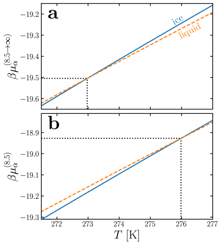
Figure 4: Locating coexistence: $\beta\mu_{\alpha}(T)$ at 0 bar, with $\alpha=\text{`ice' or `liq'}$, for (a) TIP4P/ice^(8.5→∞) and (b) TIP4P/ice^(8.5). $T_{\rm m}$ is determined from the point of interception, as indicated by the black dotted lines, with $T^{(8.5\to\infty)}_{\rm m}=273.0$ K and $T^{(8.5)}_{\rm m}=276.0$ K.

In Fig. 4a, we present $\beta\mu^{(8.5\to\infty)}_{\rm ice}(T)$ and $\beta\mu^{(8.5\to\infty)}_{\rm liq}(T)$, from which we determine $T^{(8.5\to\infty)}_{\rm m}\approx 273.0$ K. This is in good agreement with $T^{(8.5\to\infty)}_{\rm m}=272\pm 6$ K at $p=1$ bar obtained by Vega and co-workers Vega, Sanz, and Abascal (2005); Abascal et al. (2005). The results for TIP4P/ice^(8.5) are shown in Fig. 4b. It is clear that using $U^{(r_{\rm c})}$ instead of $U^{(r_{\rm c}\to\infty)}$ results in an apparent increase of the melting temperature, with $T^{(8.5)}_{\rm m}\approx 276.0$ K. While an increase of approximately $3$ K is modest, it is nonetheless comparable to the difference in melting temperature between D2O and H2O Bartholomé and Clnsins (1935); Reinhardt and Cheng (2021).

We have not reported an error estimate for either $T^{(8.5\to\infty)}_{\rm m}$ or $T_{\rm m}^{(8.5)}$. Yet, the similarity of the slopes for $\beta\mu_{\rm liq}$ and $\beta\mu_{\rm ice}$ seen in Fig. 4 suggest that even small statistical errors in the chemical potential will result in relatively large changes in the estimate of the melting temperature. Instead of performing a thorough error analysis, in Sec. III we use a combination of a MF approach and Hamiltonian Gibbs-Duhem integration Agrawal and Kofke (1995a, b) to argue that the difference in $T_{\rm m}$ reported above reflects a genuine effect of the choice of truncation schemes.

III A mean field estimate for $r_{\rm c}$ dependence of $T_{\rm m}$

We have already seen in Fig. 3a that the density of the homogeneous system under isothermal-isobaric conditions is sensitive to the choice of $U^{(r_{\rm c})}$ vs. $U^{(r_{\rm c}\to\infty)}$. As indicated by the solid blue line, $\bar{\rho}_{\rm m}(p)$ is well-described by a quadratic polynomial $r_{2}p^{2}+r_{1}p+r_{0}$ (see SM). Using this polynomial approximation in combination with Eqs. 6 and 9, we can predict the pressure difference between the $U^{(r_{\rm c})}$ and $U^{(r_{\rm c}\to\infty)}$ systems, as shown by the dashed lines in Fig. 3a. To validate this MF estimate, we have performed $NpT$ simulations for TIP4P/ice^(8.5) at $p=p^{(8.5)}$ predicted by Eq. 9. Excellent agreement between the simulation data and MF estimate is observed. This result is perhaps unsurprising, and simply reflects that $r_{\rm c}=8.5\,{\rm\AA}\approx 2.7\sigma$ is sufficiently large to ensure $g_{\rm OO}(r_{\rm c})\approx 1$. Nonetheless, it serves as an acute reminder of the effects of the truncation scheme: $\bar{\rho}_{\rm m}(p=0)$ for TIP4P/ice^(8.5) corresponds to $p\approx-427$ bar for TIP4P/ice^(8.5→∞); even for a relatively large cutoff $r_{\rm c}=14\,{\rm\AA}\approx 4.4\sigma$, differences on the order 100 bar persist.

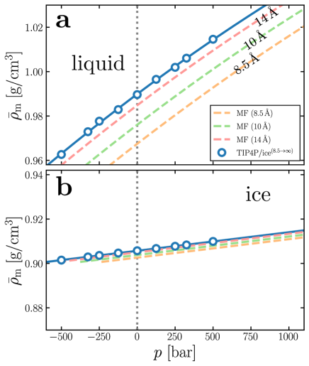
Figure 5: $\bar{\rho}_{\rm m}(p)$ at 272 K for (a) liquid water and (b) ice. White-filled circles show results from constant-$p$ simulations of TIP4P/ice^(8.5→∞), and the solid blue line indicates a quadratic fit. Dashed lines indicate MF predictions (Eq. 9) for different $r_{\rm c}$, as indicated in the legend, which are used to predict $\bar{\rho}_{\rm m}(p=0)$ for a given $r_{\rm c}$, i.e., where the dashed lines intersect the vertical gray dotted line.

Assuming that $a_{\rm LJ,ex}^{(r_{\rm c}\to\infty)}\approx a_{\rm LJ,ex}^{(\infty)}$, the Helmholtz free energy per particle for a system with potential energy function $U^{(r_{\rm c})}$ can be estimated at a MF levelJohnson, Zollweg, and Gubbins (1993),

$$a_{\rm liq}^{(r_{\rm c})}\approx a_{\rm liq}^{(r_{\rm c}\to\infty)}+\Delta_{\rm MF}a(r_{\rm c}),$$ (13)

with

$$\Delta_{\rm MF}a(r_{\rm c})=-\frac{32\pi\bar{\rho}\epsilon\sigma^{3}}{9}\Bigg{[}\bigg{(}\frac{\sigma}{r_{\rm c}}\bigg{)}^{9}-\frac{3}{2}\bigg{(}\frac{\sigma}{r_{\rm c}}\bigg{)}^{3}\Bigg{]}.$$ (14)

While MF corrections of the kind given by Eqs. 4, 6 and 14 are strictly appropriate for systems with uniform density, such as homogeneous liquids, they are often employed for crystalline phases too, with evidence to suggest that the obtained results are reasonable Jablonka, Ongari, and Smit (2019). (Note that $\Delta_{\rm MF}a$ approximates the difference in free energy between systems employing $U^{(r_{\rm c}\to\infty)}\approx U^{(\infty)}$ and $U^{(r_{\rm c})}$. In contrast, $\Delta_{\rm MF}U$ approximately accounts for the energy neglected by simply truncating the LJ potential at $r_{\rm c}$.) In Figs. 5a and 5b we show similar analyses as Fig. 3a for the liquid and ice phases of TIP4P/ice, respectively, and temperature $T_{\rm i}=272$ K, which allow us to predict $\bar{\rho}_{\rm m}(p=0)$ for both phases of TIP4P/ice${}^{(r_{\rm c})}$. Along with Eqs. 13 and 14, this estimate of the density for a given cutoff provides a MF estimate of the chemical potential:

$$\beta\mu^{({\rm MF},r_{\rm c})}\approx\beta\mu^{(r_{\rm c}\to\infty)}+\Delta_{\rm MF}a(r_{\rm c}).$$ (15)

Note that, for simplicity, we have ignored any variation of the density with temperature. Results for $\beta\mu^{({\rm MF},8.5)}$ are shown in Fig. 6, from which we deduce a MF estimate for the melting temperature $T_{\rm m}^{({\rm MF},8.5)}=275.7$ K; this is in fair agreement with $T_{\rm m}^{(8.5)}=276.0$ K obtained from our free energy calculations.

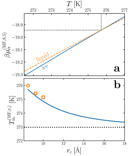
Figure 6: Predicting the effect of $r_{\rm c}$ on the melting temperature of TIP4P/ice with MF theory. (a) $\beta\mu_{\alpha}^{({\rm MF,}8.5)}(T)$ at $p=0$ bar, with $\alpha=\text{`ice' or `liq'}$, obtained from Eq. 15. $T_{\rm m}^{({\rm MF,}8.5)}=275.7$ K is determined from the point of interception, as indicated by the black dotted lines. (b) $T_{\rm m}^{({\rm MF,}r_{\rm c})}$ is shown by the solid blue line. The orange circle indicates $T_{\rm m}^{(8.5)}$ obtained from the free energy calculations described in Sec. II, and the orange squares indicate $T_{\rm m}^{(9.25)}$ and $T_{\rm m}^{(10.0)}$ obtained from Hamiltonian Gibbs-Duhem integration, starting from $T_{\rm m}^{(8.5)}$.

Without performing further simulations, we can use the above procedure to calculate $T^{({\rm MF},r_{\rm c})}_{\rm m}$ for arbitrary $r_{\rm c}$, as shown in Fig. 6b. It can be clearly seen that $T^{({\rm MF},r_{\rm c})}_{\rm m}$ approaches $T^{({\rm MF},r_{\rm c}\to\infty)}_{\rm m}$ monotonically and slowly, with differences of approximately 1 K still observed for $r_{\rm c}=12\,{\rm\AA}\approx 3.8\sigma$. Also shown in Fig. 6b are estimates of $T^{(9.25)}_{\rm m}=275.4$ K and $T^{(10.0)}_{\rm m}=275.1$ K obtained from Hamiltonian Gibbs-Duhem integration, starting from $T^{(8.5)}_{\rm m}=276.0$ K. The observed relative decrease in $T_{\rm m}$ obtained from Hamiltonian Gibbs-Duhem integration agrees well with that predicted by our MF procedure, and provides compelling evidence that reducing $r_{\rm c}$ results in a systematic increase in the melting temperature. As already mentioned, the increase in $T_{\rm m}$ with decreasing $r_{\rm c}$ is modest. We argue that this is a useful observation, as obtaining consistent ice nucleation rates among different studies has proven itself to be challengingSosso et al. (2016a). Our finding suggests that changes in the degree of supercooling due to differences in $r_{\rm c}$ are an unlikely source of significant discrepancies in nucleation rates between studies. In Sec. IV, we suggest a way in which effects of the truncation scheme can have a material impact on comparing nucleation rates.

IV Estimating the impact on ice nucleation rates

Our results so far indicate that a finite cutoff results in an increase, albeit small, on the melting temperature of SPC models of water. Despite this relatively modest effect on $T_{\rm m}$, we nonetheless anticipate that the resulting inconsistencies observed between homogeneous and inhomogeneous systems may have a significant impact when comparing nucleation rates. In particular, Figs. 3 and 5 suggest that a decrease in $r_{\rm c}$ is analogous to an increase in pressure (for fixed $\bar{\rho}$). Conversely, for inhomogeneous systems like those shown in Fig. 2b, where $U^{(r_{\rm c}\to\infty)}$ and $U^{(r_{\rm c})}$ generate the same dynamics, it is more appropriate to compare to homogeneous nucleation rates computed with $U^{(r_{\rm c}\to\infty)}$ at $p<0$ bar rather than $p=0$ bar.

To estimate the impact of this effective change in pressure arising from a finite cutoff, we appeal to the recent study of Bianco et al.Bianco et al. (2021), where homogeneous nucleation across a broad range of pressures and temperatures for TIP4P/ice^(9.0→∞) was investigated, and data for $\bar{\rho}(p)$, diffusion coefficient $D(p)$, and size of critical cluster $n_{\rm c}(p)$ were given. The homogeneous nucleation rate can then be estimated by

$$J(p)=\bar{\rho}f^{+}\mathcal{Z}\exp\big{(}-\beta\Delta G_{\rm c}\big{)},$$ (16)

where $\mathcal{Z}=\sqrt{\beta|\Delta\mu|/(6\pi n_{\rm c})}$ and $f^{+}=24Dn_{\rm c}^{2/3}/(3.8\,{\rm\AA})^{2}$. For simplicity, we have assumed $|\Delta\mu|=0.62$ kJ/mol (see Fig. 3a of Ref. Bianco et al., 2021), independent of pressure; this is justified based on previous studies that find changes in ice/water interfacial tension dominate variations in $J$ with $p$, and is supported by our finding that $T_{\rm m}$ is only weakly affected by $r_{\rm c}$ Espinosa et al. (2016); Bianco et al. (2021). (To gauge the sensitivity of our results to this approximation, the blue shaded region in Fig. 7b encompasses predictions obtained with $0.60\,{\rm kJ/mol}\leq|\Delta\mu|\leq 0.64$ kJ/mol.) In Fig. 7a we show $\bar{\rho}(p)$ at $T=230$ K for TIP4P/ice${}^{(r_{\rm c}\to\infty)}$ from Ref. Bianco et al., 2021, along with MF estimates for TIP4P/ice^(8.5) and TIP4P/ice^(11.0). From Fig. 7a, it can clearly be seen that $\bar{\rho}(p=0)$ for TIP4P/ice^(8.5) and TIP4P/ice^(11.0) correspond to $p\approx-400$ bar and $p\approx-200$ bar, respectively. In Fig. 7b, we plot $\log_{10}\big{[}J(p)/J(0)\big{]}$ according to Eq. 16, from which we estimate that homogeneous nucleation is faster in TIP4P/ice^(8.5) and TIP4P/ice^(11.0) by approximately four and two orders of magnitude, respectively.

The implication of the preceding analysis is that enhancement due to heterogeneous nucleation may in fact be lower than previously thought. For example, Sosso et al.Sosso et al. (2016c) used a variation of the cut-and-shift potential with $r_{\rm c}\approx 11$ Å to investigate ice nucleation at 230 K in the presence of kaolinite, using FFS and TIP4P/ice. By comparing to the homogeneous nucleation rate obtained by Haji-Akbari and Debenedetti for TIP4P/ice^(8.5→∞) with FFS, an enhancement of 20 orders of magnitude was reported; we estimate this result is too high by approximately two orders of magnitude. Similarly, Haji-Akbari and Debenedetti also investigated nucleation in free standing thin films of TIP4P/ice^(8.5) water Haji-Akbari and Debenedetti (2017) and found an increase of approximately seven orders of magnitude, despite nucleation occurring in bulk-like regions; Fig. 7b suggests the nucleation rate of the reference homogeneous system at $p=-400$ bar would also be faster by approximately four orders of magnitude.

This discussion on the impact of truncation scheme on the nucleation rate is admittedly crude, and relies on the analogy that a change in $r_{\rm c}$ simply amounts to a change in pressure. In practice, it is likely that relevant quantities, e.g., ice-liquid interfacial tension, will differ between TIP4P/ice${}^{(r_{\rm c}\to\infty)}$ at $p<0$ bar and TIP4P/ice${}^{(r_{\rm c})}$ at $p=0$ bar. While the estimates presented above may provide a useful first-order approximation, they await full validation by explicit calculation of nucleation rates using consistent truncation schemes for homogeneous and inhomogeneous systems. Such calculations are, however, beyond the scope of the present article.

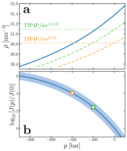
Figure 7: Estimating the impact on ice nucleation rates. (a) $\bar{\rho}(p)$ for homogeneous liquid water at 230 K. The solid blue line is the result for TIP4P/ice^(9.0→∞)Bianco et al. (2021). Dashed lines indicate MF predictions (Eq. 9) for TIP4P/ice^(8.5) (orange) and TIP4P/ice^(11.0) (green); the dotted lines indicate $\bar{\rho}(p=0)$ for these two cut-and-shift variants. For TIP4P/ice^(8.5) and TIP4P/ice^(11.0), $\bar{\rho}(p=0)$ respectively corresponds to $p\approx-400$ bar and $p\approx-200$ bar for TIP4P/ice^(9.0→∞). (b) $\log_{10}[J(p)/J(0)]$ extracted from Ref. Bianco et al., 2021 with $|\Delta\mu|=0.62$ kJ/mol. At $p\approx-400$ bar (orange circle) and $p\approx-200$ bar (green square), homogeneous nucleation is approximately four and two orders of magnitude faster, respectively, than at $p=0$ bar.

V Summary and outlook

In this article, we have investigated the effect of truncating the Lennard-Jones potential on the melting properties at $p=0$ bar of two common water models—TIP4P/ice and TIP4P/2005—that are frequently used to study ice nucleation with molecular simulations. Specifically, we have compared results from two truncation schemes: simple truncation at $r_{\rm c}$ with ‘tail corrections’; and ‘cut-and-shift’ at $r_{\rm c}$. We have combined explicit free energy calculations, Hamiltonian Gibbs-Duhem integration, and a simple mean field analysis to show that a finite cutoff results in an increase of the melting temperature. While we have focused on TIP4P/ice and TIP4P/2005, the effects described in this article should be applicable to any reasonable SPC model of water. Moreover, while not an SPC model, we note that the coarse grained mW modelMolinero and Moore (2009)—another water model commonly used to investigate ice nucleation—is inherently short-ranged, with intermolecular interactions that vanish beyond 4.32 Å. As such, we can conclude that the mW model will not suffer from the inconsistencies between homogeneous and inhomogeneous systems discussed in this article.

Based on recent work that has investigated homogeneous ice nucleation at negative pressures Bianco et al. (2021), we suggest that enhancements due to heterogeneous nucleation calculated by molecular simulations have likely been overestimated by several orders of magnitude. Going forward, those simulating heterogeneous nucleation either need to employ a truncation scheme that effectively samples $U^{(r_{\rm c}\to\infty)}$in’t Veld, Ismail, and Grest (2007); Alejandre and Chapela (2010); López-Lemus and Alejandre (2002, 2003); Míguez, Piñeiro, and Blas (2013); Janeček (2006); Salomons and Mareschal (1991); Guo, Peng, and Lu (1997); Guo and Lu (1997); de Gregorio et al. (2012), or reference data for homogeneous nucleation rates for $U^{(r_{\rm c})}$-based SPC models needs to be computed explicitly. As a stop-gap solution, one can use the crude but cheap estimate for the impact on comparing homogeneous and heterogeneous nucleation rates outlined in this article.

Inconsistencies arising from the choice of truncation scheme are not the only challenges faced when comparing homogeneous and heterogeneous ice nucleation. In particular, we note that Haji-Akbari has shown that conventional FFS approaches can underestimate nucleation rates by failing to account for the ‘jumpiness’ of the order parameter, the severity of which is system dependent Haji-Akbari (2018). While such subtleties in rate calculations further complicate quantitative comparison of homogeneous and heterogeneous nucleation rates, our work nonetheless provides an important contribution toward resolving inconsistencies between homogeneous and inhomogeneous systems. Our results will also facilitate consistent comparison of different studies of heterogeneous ice nucleation.

VI Methods

Full details of the methods used are given in the SM. In brief, molecular dynamics simulations were performed with the LAMMPS simulations package Plimpton (1995). The particle-particle particle-mesh Ewald method was used to account for long-ranged interactions Hockney and Eastwood (1988), with parameters chosen such that the root mean square error in the forces were a factor $10^{5}$ smaller than the force between two unit charges separated by a distance of 0.1 nm Kolafa and Perram (1992). For simulations of a liquid water slab in contact with its vapor, the electric displacement field along $z$ was set to zero, using the implementation given in Refs. Cox and Sprik, 2019; Sayer and Cox, 2019; this is formally equivalent to the commonly used slab correction of Yeh and Berkowitz Yeh and Berkowitz (1999). The geometry of the water molecules was constrained using the RATTLE algorithm Andersen (1983). Where appropriate, temperature was maintained with either a Nosé-Hoover chain thermostat Shinoda, Shiga, and Mikami (2004); Tuckerman et al. (2006) or Langevin dynamics Dünweg and Paul (1991); Schneider and Stoll (1978), and pressure with a Parrinello-Rahman barostat Parrinello and Rahman (1981) with a damping constant 2 ps. A time step of 2 fs was used throughout. Ice structures were generated using the GenIce software package Matsumoto, Yagasaki, and Tanaka (2018).

Supplementary Material

Supplementary Material includes a detailed overview of the simulation methods used. Results for the TIP4P/2005 water model are also given.

Data Availability Statement

The data that supports the findings of this study, analysis scripts, and input files for the simulations are openly available at the University of Cambridge Data Repository, https://doi.org/10.17863/CAM.80092.

Supplementary Material

S1 Background theory for calculating the free energy of the liquid and crystalline phases

To help set notation, and highlight slight differences in approach compared to previous studies, we will briefly cover some of the theory underlying the free energy calculations performed in the main article.

S1.1 Liquid

As we consider rigid water molecules, the position of all atoms in molecule $i$ can be specified entirely by the location of its oxygen atom $\mathbf{r}_{i}^{\rm(O)}\equiv\mathbf{R}_{i}$ and its orientation $\bm{\Omega}_{i}$. The translational and rotational momentum of molecule $i$ are denoted $\mathbf{p}_{i}$ and $\mathbf{L}_{i}$, respectively. The partition function for a system comprising $N$ indistinguishable molecules can thus be written as

$$Q =\frac{1}{h^{6N}N!}\int\!\mathrm{d}\mathbf{p}^{N}\,\int\!\mathrm{d}\mathbf{L}^{N}\,\int\!\mathrm{d}\mathbf{R}^{N}\int\!\mathrm{d}\mathbf{\Omega}^{N}\mathrm{e}^{-\beta\mathcal{K}_{\rm t}(\mathbf{p}^{N})}\mathrm{e}^{-\beta\mathcal{K}_{\rm r}(\mathbf{L}^{N})}\mathrm{e}^{-\beta\mathcal{U}(\mathbf{R}^{N},\bm{\Omega}^{N})},$$ (S1)

$$=\frac{(8\pi^{2})^{N}V^{N}}{h^{6N}N!}\int\!\mathrm{d}\mathbf{p}^{N}\,\mathrm{e}^{-\beta\mathcal{K}_{\rm t}(\mathbf{p}^{N})}\int\!\mathrm{d}\mathbf{L}^{N}\,\mathrm{e}^{-\beta\mathcal{K}_{\rm r}(\mathbf{L}^{N})}\frac{1}{V^{N}}\int\!\mathrm{d}\mathbf{R}^{N}\frac{1}{(8\pi^{2})^{N}}\int\!\mathrm{d}\mathbf{\Omega}^{N}\mathrm{e}^{-\beta\mathcal{U}(\mathbf{R}^{N},\bm{\Omega}^{N})},$$ (S2)

where $h^{6N}$ defines a volume element in phase space, $\mathcal{K}_{\rm t}$ and $\mathcal{K}_{\rm r}$ are the translational and rotational kinetic energy, respectively, and $\mathcal{U}$ is the potential energy. For non-linear rigid molecules like the water models considered,

$$\mathcal{K}_{\rm r}(\mathbf{L})=\sum_{i=1}^{N}\frac{|\mathbf{L}_{i}^{(1)}|^{2}}{2I^{(1)}}+\frac{|\mathbf{L}_{i}^{(2)}|^{2}}{2I^{(2)}}+\frac{|\mathbf{L}_{i}^{(3)}|^{2}}{2I^{(3)}},$$ (S3)

where the superscripts indicate different principal axes of rotation, and $I^{(1)}$ indicates the moment of inertia around axis 1 etc. The ideal contribution to the partition function is then

$$Q_{\rm id}=\frac{(8\pi^{2})^{N}V^{N}}{\Lambda^{3N}N!}\bigg{(}\frac{2\pi k_{\rm B}TI^{(1)}}{h^{2}}\bigg{)}^{N/2}\bigg{(}\frac{2\pi k_{\rm B}TI^{(2)}}{h^{2}}\bigg{)}^{N/2}\bigg{(}\frac{2\pi k_{\rm B}TI^{(3)}}{h^{2}}\bigg{)}^{N/2}.$$ (S4)

If the total mass of a molecule is $m$, then we can write e.g.,

$$\bigg{(}\frac{2\pi mk_{\rm B}T}{h^{2}}\bigg{)}^{N/2}\bigg{(}\frac{I^{(1)}}{m}\bigg{)}^{N/2}=\frac{1}{\Lambda^{N}}\bigg{(}\frac{I^{(1)}}{m}\bigg{)}^{N/2}.$$

Thus,

$$\ln Q_{\rm id}\approx N\ln\bigg{(}\frac{V}{N\Lambda^{3}}\bigg{)}+N$$

$$+ N\ln\bigg{[}\bigg{(}\frac{I^{(1)}}{m}\bigg{)}^{1/2}\frac{1}{\Lambda}\bigg{]}+N\ln\bigg{[}\bigg{(}\frac{I^{(2)}}{m}\bigg{)}^{1/2}\frac{1}{\Lambda}\bigg{]}+N\ln\bigg{[}\bigg{(}\frac{I^{(3)}}{m}\bigg{)}^{1/2}\frac{1}{\Lambda}\bigg{]}+N\ln 8\pi^{2}$$ (S5)

$$=-N\ln\big{(}\bar{\rho}\Lambda^{3}\big{)}+N-N\ln\bigg{[}\bigg{(}\frac{m^{3}}{I^{(1)}I^{(2)}I^{(3)}}\bigg{)}^{1/2}\frac{\Lambda^{3}}{8\pi^{2}}\bigg{]},$$ (S6)

$$=-N\ln\big{(}\bar{\rho}\eta_{\rm r}\Lambda^{6}\big{)}+N,$$ (S7)

where we have defined

$$\eta_{\rm r}\equiv\bigg{(}\frac{m^{3}}{I^{(1)}I^{(2)}I^{(3)}}\bigg{)}^{1/2}\frac{1}{8\pi^{2}}.$$

Let us now write $\eta_{\rm r}^{1/6}\Lambda=\bar{\Lambda}_{0}T^{-1/2}$, such that $\bar{\Lambda}_{0}T_{0}^{-1/2}=1$ Å^1/2. Then,

$$\eta_{\rm r}^{1/6}\Lambda=\bar{\Lambda}_{0}T_{0}^{-1/2}\bigg{(}\frac{T_{0}}{T}\bigg{)}^{1/2}=\bigg{(}\frac{T_{0}}{T}\bigg{)}^{1/2}\,\text{\AA}^{1/2}.$$

The ideal free energy can then be written as,

$$\frac{\beta A_{\rm id}}{N}=\beta a_{\rm id}=\ln\big{(}\bar{\rho}(T_{0}/T)^{3}\big{)}-1,$$ (S8)

where it is understood that $(T_{0}/T)$ carries units of Å. The choice of reference temperature $T_{0}$ is arbitrary provided it is chosen consistently. This approach differs from the common ‘set $\Lambda=1$ Å’ encountered in the literature Vega et al. (2008). By adopting this approach we use, e.g., the full enthalpy when performing thermodynamic integration (c.f. Ref. Reinhardt, 2019).

The excess part of the partition function is

$$Q_{\rm ex}=\frac{1}{(8\pi^{2}V)^{N}}\int\!\mathrm{d}\mathbf{R}^{N}\int\!\mathrm{d}\mathbf{\Omega}^{N}\mathrm{e}^{-\beta\mathcal{U}(\mathbf{R}^{N},\bm{\Omega}^{N})}.$$ (S9)

Note that, if $\mathcal{U}$ is independent of $\Omega$ e.g., we turn off the charges in our water model, then $Q_{\rm ex}$ reduces to that of a simple mono-atomic system. This means we are free to use equations of state for the standard LJ liquid where appropriate; we make use of this fact to calculate the excess free energy of the liquid by thermodynamic integration.

S1.2 Ice

Unlike liquid water, the molecules in the crystalline phase are distinguishable by virtue of their association with a particular set of lattice sites. This leads to a straightforward modification of the partition function:

$$Q=\frac{1}{h^{6N}}\int\!\mathrm{d}\mathbf{p}^{N}\,\int\!\mathrm{d}\mathbf{L}^{N}\,\int\!\mathrm{d}\mathbf{R}^{N}\int\!\mathrm{d}\mathbf{\Omega}^{N}\mathrm{e}^{-\beta\mathcal{K}_{\rm t}(\mathbf{p}^{N})}\mathrm{e}^{-\beta\mathcal{K}_{\rm r}(\mathbf{L}^{N})}\mathrm{e}^{-\beta\mathcal{U}(\mathbf{R}^{N},\bm{\Omega}^{N})}$$ (S10)

Instead of dealing with ‘ideal’ and ‘excess’ quantities, it is now useful to consider ‘kinetic’ and ‘configurational’ quantities:

$$Q_{\rm kin} =\frac{1}{\Lambda^{6N}\eta_{\rm r}^{N}},$$ (S11)

$$Q_{\rm con} =\frac{1}{(8\pi^{2})^{N}}\int\!\mathrm{d}\mathbf{r}_{\rm O}^{N}\int\!\mathrm{d}\mathbf{\Omega}^{N}\mathrm{e}^{-\beta\mathcal{U}(\mathbf{r}_{\rm O}^{N},\bm{\Omega}^{N})}.$$ (S12)

Note that $Q_{\rm kin}$ and $Q_{\rm con}$ have dimensions of hyperdensity and hypervolume, respectively; it is important that units are chosen consistently. The factor $1/(8\pi^{2})^{N}$ is still included in $Q_{\rm con}$ to ensure a consistent definition of $\eta_{r}$. By similar reasoning to above, we can write the kinetic contribution to the free energy as

$$\frac{\beta A_{\rm kin}}{N}=\beta a_{\rm kin}=\ln\big{(}(T_{0}/T)^{3}\big{)}.$$ (S13)

As detailed below, we have used the Frenkel-Ladd approach Frenkel and Ladd (1984), adapted by Vega and co-workers for rigid SPC water models Noya, Conde, and Vega (2008); Vega et al. (2008); Aragones et al. (2013), to calculate the difference in free energy between a non-interacting crystal with its atoms tethered to their equilibrium positions by harmonic springs, and the fully interacting crystal. The potential energy of the former, ‘reference’, system is

$$\mathcal{U}_{\rm ref}(\mathbf{R}^{N},{\bm{\Omega}}^{N})=\sum_{i}^{N}\sum_{\alpha}\frac{k^{(\alpha)}}{2}\big{(}\mathbf{R}_{i}+\Delta\mathbf{r}_{i}^{(\alpha)}({\bm{\Omega}_{i}})-\mathbf{r}_{i}^{(\alpha,0)}\big{)}^{2},$$ (S14)

where $\Delta\mathbf{r}_{i}^{(\alpha)}=\mathbf{r}_{i}^{(\alpha)}-\mathbf{R}_{i}$, $\mathbf{r}_{i}^{(\alpha,0)}$ is the equilibrium position of atom $\alpha$ of molecule $i$ (recall that $\mathbf{r}_{i}^{\rm(O)}\equiv\mathbf{R}_{i}$), and $k^{(\alpha)}$ determines the strength of the harmonic potential that tethers atom $\alpha$ to $\mathbf{r}_{i}^{(\alpha,0)}$. The rigid body constraints mean that the free energy of this reference system is analytically intractable. We therefore define a ‘sub-reference’ system with the following potential energy,

$$\mathcal{U}_{\rm sub}(\mathbf{R}^{N})=\sum_{i}^{N}\frac{k^{\rm(O)}}{2}\big{(}\mathbf{r}^{\rm(O)}_{i}-\mathbf{r}_{i}^{({\rm O},0)}\big{)}^{2}.$$ (S15)

The configurational partition function for this sub-reference system is just that of the standard Einstein crystal,

$$Q_{\rm sub}=\int\!\mathrm{d}\mathbf{R}^{N}\exp\left(-\beta\mathcal{U}_{\rm sub}(\mathbf{R}^{N})\right),$$ (S16)

resulting in the following free energy per particle:

$$\beta a_{\rm sub}=-\frac{3}{2}\ln\bigg{(}\frac{2\pi}{\beta k^{\rm(O)}}\bigg{)}.$$ (S17)

S2 Workflow: Free energy calculations of ice I_h

The procedure described below was performed for both truncation schemes described in the main article and both water models, i.e., for TIP4P/ice^(8.5→∞), TIP4P/ice^(8.5), TIP4P/2005^(8.5→∞), and TIP4P/2005^(8.5). Unless otherwise stated, all simulations used the LAMMPS simulation package Plimpton (1995). The particle-particle particle-mesh Ewald method was used to account for long-ranged interactions Hockney and Eastwood (1988), with parameters chosen such that the root mean square error in the forces were a factor $10^{5}$ smaller than the force between two unit charges separated by a distance of 0.1 nm Kolafa and Perram (1992). The geometry of the water molecules was constrained using the RATTLE algorithm Andersen (1983). A time step of 2 fs was used throughout.

S2.1 Obtaining average cell parameters

A proton disordered ice I_h structure comprising 768 molecules was generated using the GenIce software package Matsumoto, Yagasaki, and Tanaka (2018). After equilibration of at least 0.5 ns, the average cell parameters were obtained from a 10 ns simulation at $p=0$ bar and temperature $T=T_{\rm i}$, with $T_{\rm i}=272$ K for TIP4P/ice, and $T_{\rm i}=252$ K for TIP4P/2005. Temperature was maintained with a Nosé-Hoover chain thermostat Shinoda, Shiga, and Mikami (2004); Tuckerman et al. (2006) with a damping constant 0.2 ps, and the pressure was maintained with a Parrinello-Rahman barostat Parrinello and Rahman (1981) with a damping constant 2 ps. The latter was applied such that all cell lengths and angles could fluctuate independently.

S2.2 Obtaining the reference ice structure

The simulation cell parameters were fixed to their average values, and the structure was ‘minimized’ by running short (approximately 10-20 ps) simulations at $T=0.1$ K. The damping constant of the Nosé-Hoover chain thermostat was reduced to 20 fs. As explained in the main text, this approach was adopted as standard minimizers available in LAMMPS are incompatible with the RATTLE algorithm used to constrain the rigid geometry of the water molecules. Simulation settings were otherwise the same as above.

S2.3 Thermodynamic integration from the non-interacting to interacting crystal

Atoms were tethered to their positions in the reference ice structure with force constants $k^{\rm(O)}=4.8$ kcal/mol-Ų and $k^{\rm(H)}=6.0$ kcal/mol-Ų (see Sec. S1.2). For each water model and truncation scheme considered, we constructed the following potential energy function:

$$\mathcal{U}_{\lambda}(\mathbf{R}^{N},{\bm{\Omega}}^{N})=\lambda\mathcal{U}(\mathbf{R}^{N},{\bm{\Omega}}^{N})+(1-\lambda)\mathcal{U}_{\rm ref}(\mathbf{R}^{N},{\bm{\Omega}}^{N}),$$ (S18)

where $\mathcal{U}$ is replaced with $U^{(r_{\rm c}\to\infty)}$ or $U^{(r_{\rm c})}$ as appropriate (see Eqs. I.1 and 8). The Helmholtz free energy difference between the reference and interacting systems is then,

$$\Delta_{\rm r2i}a=\frac{1}{N}\int_{0}^{1}\!\mathrm{d}\lambda\,\langle\Delta U(\mathbf{R}^{N},{\bm{\Omega}}^{N})\rangle_{\lambda},$$ (S19)

where $\Delta U(\mathbf{R}^{N},{\bm{\Omega}}^{N})=\mathcal{U}(\mathbf{R}^{N},{\bm{\Omega}}^{N})-\mathcal{U}_{\rm ref}(\mathbf{R}^{N},{\bm{\Omega}}^{N})$, and $\langle\cdots\rangle_{\lambda}$ denotes a canonical ensemble average according to the Hamiltonian specified by $\mathcal{U}_{\lambda}$. The integral in Eq. S19 was evaluated using 11-point Gauss-Legendre quadrature, and simulations for each value of $\lambda$ were 20 ns in length. Temperature was maintained through Langevin dynamics as implemented in LAMMPS Dünweg and Paul (1991); Schneider and Stoll (1978), with a damping constant 100 fs. The total random force was set exactly to zero to ensure the center-of-mass of the system did not drift.

S2.4 Thermodynamic integration from the sub-reference to reference system

As molecules in both the sub-reference and reference systems are non-interacting, we need only consider the behavior of a single water molecule. Specifically, we construct the following energy function:

$$u_{\lambda}(\mathbf{R}_{1},{\bm{\Omega}}_{1})=\lambda\mathcal{U}^{(N=1)}_{\rm ref}(\mathbf{R}_{1},{\bm{\Omega}}_{1})+(1-\lambda)\mathcal{U}^{(N=1)}_{\rm sub}(\mathbf{R}_{1},{\bm{\Omega}}_{1}),$$ (S20)

where $\mathcal{U}^{(N=1)}_{\rm ref}$ and $\mathcal{U}^{(N=1)}_{\rm sub}$ are given by Eqs. S14 and S15 with $N=1$. The change in Helmholtz free energy is then given by:

$$\Delta_{\rm s2r}a=\int_{0}^{1}\!\mathrm{d}\lambda\,\langle\Delta u(\mathbf{R}^{N},{\bm{\Omega}}^{N})\rangle_{\lambda},$$ (S21)

with $\Delta u=\mathcal{U}^{(N=1)}_{\rm ref}-\mathcal{U}^{(N=1)}_{\rm sub}$, and $\langle\cdots\rangle_{\lambda}$ now denotes a canonical ensemble average at temperature $T_{\rm i}$ according to the Hamiltonian specified by $u_{\lambda}$. The integral in Eq. S21 was again evaluated using 11-point Gauss-Legendre quadrature, using a bespoke Metropolis Monte Carlo (MC) code. In brief, after $10^{4}$ MC moves for equilibration, production simulations of $5\times 10^{7}$ MC moves were performed for each value of $\lambda$. For each MC move, the water molecule was either translated or rotated with equal probability. For translations, a displacement along each Cartesian direction was randomly chosen in the interval $[-\sqrt{2/\beta k^{\rm(O)}},\sqrt{2/\beta k^{\rm(O)}})$. For rotations, three angles ($\alpha,\beta,\gamma$) were randomly chosen in the interval $[0,\pi/6)$, and a rotation matrix was constructed as $\mathbf{R}=\mathbf{R}_{z}(\alpha)\mathbf{R}_{y}(\beta)\mathbf{R}_{x}(\gamma)$, where $\mathbf{R}_{x}(\gamma)$ is a rotation about the $x$-axis etc. With equal probability, the molecule was then rotated about its oxygen position using either $\mathbf{R}$ or its transpose. Note that, as $\Delta_{\rm s2r}a$ is independent of truncation scheme, we only computed it once for each water model.

S2.5 Computing $\beta\mu_{\rm ice}(T)$

With an estimate of $\beta_{\rm i}\mu_{\rm ice}(T_{\rm i})$ obtained from thermodynamic integration, $\beta\mu_{\rm ice}(T)$ is computed from the Gibbs-Helmholtz relation (Eq. 12). For TIP4P/ice^(8.5→∞) and TIP4P/ice^(8.5), simulations in the temperature range $T=267\,{\rm K},268\,{\rm K},\ldots,277\,{\rm K}$, and $T=267\,{\rm K},268\,{\rm K},\ldots,282\,{\rm K}$, respectively, were performed, while for TIP4P/2005^(8.5→∞) and TIP4P/2005^(8.5) we adopted the temperature range $T=247\,{\rm K},248\,{\rm K},\ldots,267\,{\rm K}$. Simulations were initialized from the reference structure, starting at 0.1 K with the temperature steadily increased to $T$ over 1 ns at constant volume. An equilibration period of 0.5 ns at constant $T$ and $p=0$ bar was then performed (see Sec. S2.1), followed by a production run of 20 ns. The integrand in Eq. 12 was then fitted to a quadratic polynomial, from which $\beta\mu_{\rm ice}(T)$ was obtained by analytic integration.

S3 Workflow: Free energy calculations of liquid water

The procedure described below is again appropriate for both truncation schemes and both water models. Simulation details were broadly similar to those specified throughout Sec. S2.

S3.1 Obtaining the average density of liquid water

A 20 ns simulation of liquid water was performed after at least 0.5 ns equilibration at temperature $T_{\rm i}$ and $p=0$ bar. A Nosé-Hoover chain thermostat was used to maintain the temperature, and an isotropic Parrinello-Rahman barostat was used to maintain the pressure.

S3.2 Thermodynamic integration from the LJ fluid to water

To compute the excess free energy of liquid water, we exploit the fact that the equation of state for the LJ fluid has been computed previously, which provides $a^{(r_{\rm c}\to\infty)}_{\rm LJ,ex}$. The density of the fluid is fixed to its average (see Sec. S3.1) at temperature $T_{\rm i}$ and $p=0$ bar, and thermodynamic integration is performed with the following energy function:

$$\mathcal{U}_{\lambda}(\mathbf{R}^{N},{\bm{\Omega}}^{N})=\mathcal{U}(\mathbf{R}^{N},{\bm{\Omega}}^{N})\text{ with charges multiplied by $\lambda^{1/2}$.}$$ (S22)

(We reuse the notation $\mathcal{U}_{\lambda}$ as it should be clear from context what is intended.) Again, $\mathcal{U}$ is replaced with $U^{(r_{\rm c}\to\infty)}$ or $U^{(r_{\rm c})}$ as appropriate. The free energy difference $\Delta_{\rm LJ2w}a$ between water and the LJ fluid is then given by an expression analogous to Eq. S19, with the integral evaluated by 9-point Gauss-Legendre quadrature. For each value of $\lambda$, $\langle\Delta U(\mathbf{R}^{N},{\bm{\Omega}}^{N})\rangle_{\lambda}$ was averaged over a 20 ns simulation, following a 0.5 ns equilibration period.

S3.3 Thermodynamic integration from the ‘truncated + tail corrections’ LJ fluid to ‘cut-and-shift’ LJ fluid

For systems employing the ‘cut-and-shift’ truncation scheme, we also computed the free energy difference between the fluid with interactions described by $u_{\rm LJ}^{(r_{\rm c}\to\infty)}$ and $u_{\rm LJ}^{(r_{\rm c})}$. As dynamics in the canonical ensemble are unaffected by this choice of truncation scheme, we simply have (see Eq. S22)

$$\Delta_{\rm tc2cs}a=\big{\langle}U_{\lambda=0}^{(8.5)}(\mathbf{R}^{N},{\bm{\Omega}}^{N})-U_{\lambda=0}^{(8.5\to\infty)}(\mathbf{R}^{N},{\bm{\Omega}}^{N})\big{\rangle},$$ (S23)

which we calculated from a 20 ns simulation, following a 0.5 ns equilibration period.

S3.4 Computing $\beta\mu_{\rm liq}(T)$

Using the same temperature ranges described in Sec. S2.5, the Gibbs-Helmholtz equation was evaluated in an analogous manner to $\beta\mu_{\rm ice}(T)$. For each temperature, a 0.5 ns equilibration period was performed followed by a 20 ns production run. The pressure was maintained with an isotropic barostat (see Sec. S3.1).

S4 Workflow: Locating the melting point

For each water model and truncation scheme, $\beta\mu_{\rm ice}(T)$ and $\beta\mu_{\rm liq}(T)$ were each fitted to a quadratic polynomial, and the melting temperature was obtained by solving the resulting simultaneous equations.

S5 Workflow: Hamiltonian Gibbs-Duhem integration

With $T_{\rm m}^{(8.5)}$ determined from the free energy approach described above, $T_{\rm m}^{(9.25)}$ and $T_{\rm m}^{(10.0)}$ were subsequently determined by Hamiltonian Gibbs-Duhem integration. Specifically, we define the potential energy function

$$U_{\lambda}(\mathbf{R}^{N},{\bm{\Omega}}^{N})=\lambda U^{(r_{{\rm c},1})}(\mathbf{R}^{N},{\bm{\Omega}}^{N})+(1-\lambda)U^{(r_{{\rm c},0})}(\mathbf{R}^{N},{\bm{\Omega}}^{N}),$$ (S24)

and the quantity,

$$x^{(\lambda)}_{\alpha}=\frac{1}{N}\big{\langle}U^{(r_{{\rm c},1})}(\mathbf{R}^{N},{\bm{\Omega}}^{N})-U^{(r_{{\rm c},0})}(\mathbf{R}^{N},{\bm{\Omega}}^{N})\big{\rangle}_{\lambda},$$ (S25)

where $\alpha$ indicates sampling of the ice or liquid phase. The derivative of the melting temperature with respect to $\lambda$ is then

$$\frac{\mathrm{d}T_{\rm m}^{(r_{{\rm c},\lambda})}}{\mathrm{d}\lambda}=\frac{T\big{(}x^{(\lambda)}_{\rm ice}-x^{(\lambda)}_{\rm liq}\big{)}}{h^{(\lambda)}_{\rm ice}-h^{(\lambda)}_{\rm liq}},$$ (S26)

where $h^{(\lambda)}_{\rm ice}$ and $h^{(\lambda)}_{\rm liq}$ are the enthalpies per particle of ice and liquid, respectively, obtained from trajectories using $U_{\lambda}$. Starting from $T_{\rm m}^{(8.5)}$, $T_{\rm m}^{(9.25)}$ was obtained by integrating Eq. S26 by fourth-order Runge-Kutta integration. This was then repeated, starting from $T_{\rm m}^{(9.25)}$, to obtain an estimate for $T_{\rm m}^{(10.0)}$. We implemented $U_{\lambda}$ by tabulating the potential at 0.0005 Å intervals for $1.8\,{\rm\AA}<r<10.1\,{\rm\AA}$, but otherwise, simulation settings were the same as those described in Secs. S2.1 and S3.1. Simulations were 5 ns, following 0.5 ns equilibration.

S6 Workflow: Liquid-vapor simulations

Simulations to produce Figs. 3b and S1b comprised 512 water molecules, using TIP4P/ice and TIP4P/2005, respectively. Simulation details are broadly similar to those described in S3. The cross sectional ($xy$) area of the simulation box was $19.7\times 19.7$ Ų, and its length normal ($z$) to the liquid-vapor interface was 90 Å. To facilitate post-processing analysis, repulsive walls as described in Ref. Cox, 2020 were placed at the edges of the simulation cell along $z$ to prevent molecules escaping the primary simulation cell. The electric displacement field along $z$ was set to zero, using the implementation given in Refs. Cox and Sprik, 2019; Sayer and Cox, 2019; this is formally equivalent to the commonly used slab correction of Yeh and Berkowitz Yeh and Berkowitz (1999). Production simulations were performed for 20 ns following at least 0.5 ns equilibration. A Nosé-Hoover chain thermostat was used to maintain the temperature at 300 K. ‘Tail corrections’ were formally applied, but as discussed in the main text, this produces the same dynamics as the ‘cut-and-shift’ potential.

S7 Results for TIP4P/2005

In this section, we present results obtained with TIP4P/2005. While quantitative differences are expected, and indeed observed, our general conclusions are unaffected by the choice of water model. At $p=0$ bar, we find $T_{\rm m}^{(8.5\to\infty)}=251.9$ K in good agreement with $T_{\rm m}=252\pm 6$ K reported previously for $p=1$ bar. We also see a modest increase in melting temperature when using TIP4P/2005^(8.5), with $T_{\rm m}^{(8.5)}=253.4$ K and $T_{\rm m}^{({\rm MF,}8.5)}=254.0$ K. The predictions of the mean-field prediction are supported by Hamiltonian Gibbs-Duhem integration. Note that, unlike the results for TIP4P/ice${}^{(r_{\rm c})}$ reported in the main paper (Fig. 5b), the Hamiltonian Gibbs-Duhem simulations performed for TIP4P/2005${}^{(r_{\rm c})}$ were initiated from $T_{\rm m}^{({\rm MF,}8.5)}$ instead of $T_{\rm m}^{(8.5)}$ (indicated by the blue star in Fig. S4).

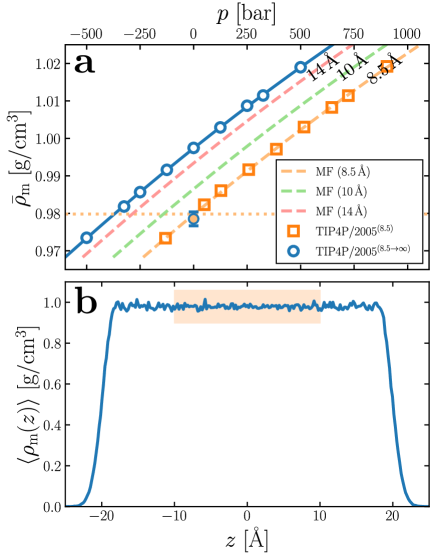
Figure S1: Evaluating the impact of $r_{\rm c}$ on $\bar{\rho}_{\rm m}$ for liquid TIP4P/2005 at 300 K. (a) $\bar{\rho}_{\rm m}(p)$ for a homogeneous system. White-filled circles show results from constant-$p$ simulations of TIP4P/2005^(8.5→∞), and the solid blue line indicates a quadratic fit. Dashed lines indicate MF predictions (Eq. 9) for different $r_{\rm c}$, as indicated in the legend. Orange squares show results from constant-$p$ simulations of TIP4P/2005^(8.5). The dotted line indicates $\bar{\rho}_{\rm m}(0)$ for TIP4P/2005^(8.5), which intercepts the TIP4P/2005^(8.5→∞) results at $p\approx-370$ bar. (b) $\langle\rho_{\rm m}(z)\rangle$ for a film of TIP4P/2005^(8.5→∞) in contact with its vapor (only part of the simulation cell is shown). Spatially averaging $\langle\rho_{\rm m}(z)\rangle$ in the slab’s interior, as indicated by the shaded region, gives an estimate $\bar{\rho}_{\rm m}(0)$, which is plotted with the orange-filled circle in (a).

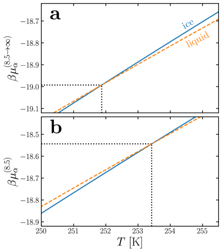
Figure S2: $\beta\mu_{\alpha}(T)$ at 0 bar, with $\alpha=\text{`ice' or `liq'}$, for (a) TIP4P/2005^(8.5→∞) and (b) TIP4P/2005^(8.5). $T_{\rm m}$ is determined from the point of interception, as indicated by the black dotted lines, with $T^{(8.5\to\infty)}_{\rm m}=251.9$ K and $T^{(8.5)}_{\rm m}=253.4$ K.

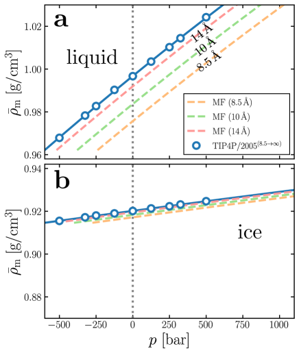
Figure S3: $\bar{\rho}_{\rm m}(p)$ at 252 K for (a) liquid water and (b) ice. White-filled circles show results from constant-$p$ simulations of TIP4P/2005^(8.5→∞), and the solid blue line indicates a quadratic fit. Dashed lines indicate MF predictions (Eq. 9) for different $r_{\rm c}$, as indicated in the legend, which are used to predict $\bar{\rho}_{\rm m}(0)$ for a given $r_{\rm c}$, i.e., where the dashed lines intersect the vertical gray dotted line.

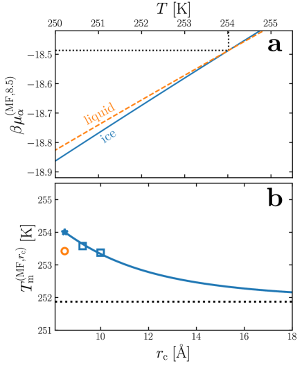
Figure S4: Predicting the effect of $r_{\rm c}$ on the melting temperature of TIP4P/2005 with MF theory. (a) $\beta\mu_{\alpha}^{({\rm MF,}8.5)}(T)$ at $p=0$ bar, with $\alpha=\text{`ice' or `liq'}$, obtained from Eq. 15. $T_{\rm m}^{({\rm MF,}8.5)}=254.0$ K is determined from the point of interception, as indicated by the black dotted lines. (b) $T_{\rm m}^{({\rm MF,}r_{\rm c})}$ is shown by the solid blue line. The orange circle indicates $T_{\rm m}^{(8.5)}$ obtained from the free energy calculations described in Sec. II, and the blue squares indicate $T_{\rm m}^{(9.25)}$ and $T_{\rm m}^{(10.0)}$ obtained from Hamiltonian Gibbs-Duhem integration, starting from $T_{\rm m}^{({\rm MF,}8.5)}$, which is marked with the blue star.

S8 Fitting coefficients

In this section, we report the coefficients for the quadratic polynomial $r_{2}p^{2}+r_{1}p+r_{0}$ obtained using numpy’s polyfit routine Harris et al. (2020), as shown in Figs. 3 and 5 in the main article, and Figs. S1 and S3.

S8.1 Results for TIP4P/ice

• Liquid, 300 K (Fig. 3a):

  • $r_{2}=-3.822428\times 10^{-9}$ g/(bar² cm³);

  • $r_{1}=4.460206\times 10^{-5}$ g/(bar cm³);

  • $r_{0}=9.939254\times 10^{-1}$ g/cm³.

• Liquid, 272 K (Fig. 5a):

  • $r_{2}=-4.700729\times 10^{-9}$ g/(bar${}^{2}\,$cm³);

  • $r_{1}=5.129812\times 10^{-5}$ g/(bar cm³);

  • $r_{0}=9.898901\times 10^{-1}$ g/cm³.

• Ice, 272 K (Fig. 5b):

  • $r_{2}=1.442316\times 10^{-11}$ g/(bar${}^{2}\,$cm³);

  • $r_{1}=8.358199\times 10^{-6}$ g/(bar cm³);

  • $r_{0}=9.056778\times 10^{-1}$ g/cm³.

S8.2 Results for TIP4P/2005

• Liquid, 300 K (Fig. S1a):

  • $r_{2}=-4.748523\times 10^{-9}$ g/(bar² cm³);

  • $r_{1}=4.561509\times 10^{-5}$ g/(bar cm³);

  • $r_{0}=9.973669\times 10^{-1}$ g/cm³.

• Liquid, 252 K (Fig. S3a):

  • $r_{2}=-3.051495\times 10^{-9}$ g/(bar${}^{2}\,$cm³);

  • $r_{1}=5.587068\times 10^{-5}$ g/(bar cm³);

  • $r_{0}=9.967701\times 10^{-1}$ g/cm³.

• Ice, 252 K (Fig. S3b):

  • $r_{2}=-2.226744\times 10^{-10}$ g/(bar${}^{2}\,$cm³);

  • $r_{1}=9.123390\times 10^{-6}$ g/(bar cm³);

  • $r_{0}=9.201753\times 10^{-1}$ g/cm³.

S9 Comment on the apparent role of impulsive forces

We have remarked in the main article that in the canoncial ensemble, dynamics are unaffected by the choice of $U^{(r_{\rm c})}$ vs. $U^{(r_{\rm c}\to\infty)}$. While we have verified this directly by comparing trajectories, and by checking the forces between a pair of LJ particles (as implemented in LAMMPS), the form of $u^{(r_{\rm c}\to\infty)}_{\rm LJ}$ given by Eq. 3 suggests the presence of an impulsive force at $r=r_{\rm c}$. Here will we demonstrate that including impulsive forces would be inconsistent with standard implementations of tail corrections.

Let us introduce a system with the following potential energy:

$$U^{(r_{\rm c}!)}(\mathbf{R}^{N})=\sum_{i<j}^{N}u^{(r_{\rm c}!)}_{\rm LJ}(|\mathbf{r}^{\rm(O)}_{ij}|)+U_{\rm elec}(\mathbf{R}^{N}),$$ (S27)

with

$$u^{(r_{\rm c}!)}_{\rm LJ}(r)=u^{(\infty)}_{\rm LJ}(r)h(r_{\rm c}-r),$$ (S28)

where $h(r)$ is the Heaviside step function. The potential energy function $U^{(r_{\rm c}!)}$ describes a system where LJ interactions are described by the unshifted LJ potential for $r\leq r_{\rm c}$, and abruptly vanish for $r>r_{\rm c}$. Forces due to the LJ interactions are obtained by differentiation,

$$f^{(r_{\rm c}!)}_{\rm LJ}(r)=f^{(\infty)}_{\rm LJ}(r)h(r_{\rm c}-r)+u^{(\infty)}_{\rm LJ}(r)\delta(r_{\rm c}-r).$$ (S29)

We clearly see an impulsive force at $r=r_{\rm c}$. Now consider the average virial pressure:

$$p^{(r_{\rm c}!)} =\frac{2\pi\bar{\rho}^{2}}{3}\int_{0}^{r_{\rm c}}\!\mathrm{d}r\,r^{3}f^{(\infty)}_{\rm LJ}(r)g(r)+\frac{2\pi\bar{\rho}^{2}}{3}r_{\rm c}^{3}u^{(\infty)}_{\rm LJ}(r_{\rm c}),$$ (S30)

$$=\frac{2\pi\bar{\rho}^{2}}{3}\int_{0}^{r_{\rm c}}\!\mathrm{d}r\,r^{3}f^{(\infty)}_{\rm LJ}(r)g(r)+\frac{8\pi\epsilon\bar{\rho}^{2}\sigma^{3}}{3}\left[\bigg{(}\frac{\sigma}{r_{\rm c}}\bigg{)}^{9}-\bigg{(}\frac{\sigma}{r_{\rm c}}\bigg{)}^{3}\right],$$ (S31)

where we have assumed that $g_{\rm OO}(r\geq r_{\rm c})=1$. The second term in Eq. S31, which we will denote $\Delta p^{(r_{\rm c}!)}$, is the impulsive contribution to the virial. For a system where impulsive forces are present (whose dynamics in the $NVT$ ensemble in principle differ from $U^{(r_{\rm c})}$ and $U^{(r_{\rm c}\to\infty)}$ systems), one is required to add $\Delta p^{(r_{\rm c}!)}$ to the virial pressure, which in turn will affect the dynamics in the $NpT$ ensemble. If we attempt to account for neglected interactions beyond the cutoff in the usual fashion by simply adding the contribution

$$\Delta_{\rm MF}p(r_{\rm c})=\frac{2\pi\bar{\rho}^{2}}{3}\int_{r_{\rm c}}^{\infty}\!\mathrm{d}r\,r^{3}f_{\rm LJ}^{(\infty)}(r)=\frac{32\pi\epsilon\bar{\rho}^{2}\sigma^{3}}{9}\Bigg{[}\bigg{(}\frac{\sigma}{r_{\rm c}}\bigg{)}^{9}-\frac{3}{2}\bigg{(}\frac{\sigma}{r_{\rm c}}\bigg{)}^{3}\Bigg{]}$$ (S32)

to $p^{(r_{\rm c}!)}$, we find an average virial pressure,

$$\frac{2\pi\bar{\rho}^{2}}{3}\int_{0}^{r_{\rm c}}\!\mathrm{d}r\,r^{3}f^{(\infty)}_{\rm LJ}(r)g(r)+\Delta p^{(r_{\rm c}!)}+\Delta_{\rm MF}p(r_{\rm c}),$$ (S33)

that does not approximately describe the average virial pressure of a $U^{(\infty)}$ system.

Now consider a $U^{(r_{\rm c}\to\infty)}$ system. The LJ pair potential is

$$u^{(r_{\rm c}\to\infty)}_{\rm LJ}(r)=u^{(\infty)}_{\rm LJ}(r)h(r_{\rm c}-r)+u^{(\infty)}_{\rm LJ}(r)h(r-r_{\rm c}),$$ (S34)

with the proviso that interactions for $r>r_{\rm c}$ are evaluated in a mean field fashion. The forces are:

$$f^{(r_{\rm c}\to\infty)}_{\rm LJ}(r) =f^{(\infty)}_{\rm LJ}(r)h(r_{\rm c}-r)+f^{(\infty)}_{\rm LJ}(r)h(r-r_{\rm c})+u^{(\infty)}_{\rm LJ}(r)\delta(r_{\rm c}-r)-u^{(\infty)}_{\rm LJ}(r)\delta(r-r_{\rm c}).$$ (S35)

The impulsive forces at $r=r_{\rm c}$ cancel. Again, we consider the average virial pressure:

$$p^{(r_{\rm c}\to\infty)} =\frac{2\pi\bar{\rho}^{2}}{3}\int_{0}^{r_{\rm c}}\!\mathrm{d}r\,r^{3}f^{(\infty)}_{\rm LJ}(r)g(r)+\Delta p^{(r_{\rm c}!)}-\Delta p^{(r_{\rm c}!)}+\Delta_{\rm MF}p(r_{\rm c}),$$ (S36)

$$=\frac{2\pi\bar{\rho}^{2}}{3}\int_{0}^{r_{\rm c}}\!\mathrm{d}r\,r^{3}f^{(\infty)}_{\rm LJ}(r)g(r)+\Delta_{\rm MF}p(r_{\rm c}).$$ (S37)

Equation S37 demonstrates that the standard ‘tail correction,’ $\Delta_{\rm MF}p$, is appropriate for a system that employs $u^{(r_{\rm c}\to\infty)}_{\rm LJ}(r)$ (Eq. 3) to describe explicit LJ interactions for $r\leq r_{\rm c}$ in which the apparent impulsive force at $r=r_{\rm c}$ is not included. In this case, dynamics in the $U^{(r_{\rm c}\to\infty)}$ and $U^{(r_{\rm c})}$ systems are identical in the $NVT$ ensemble. It would be inconsistent to use $\Delta_{\rm MF}p(r_{\rm c})$ in combination with a system whose dynamics includes impulsive forces (see S33).

References

- Tan, Storelvmo, and Zelinka (2016) I. Tan, T. Storelvmo, and M. D. Zelinka, Science 352, 224 (2016).
- Slater et al. (2016) B. Slater, A. Michaelides, C. G. Salzmann, and U. Lohmann, Bull. Amer. Meteor. Soc. 97, 1797 (2016).
- Bar Dolev, Braslavsky, and Davies (2016) M. Bar Dolev, I. Braslavsky, and P. L. Davies, Annu. Rev. Biochem. 85, 515 (2016).
- Murray et al. (2012) B. Murray, D. O’sullivan, J. Atkinson, and M. Webb, Chem. Soc. Rev. 41, 6519 (2012).
- Sosso et al. (2016a) G. C. Sosso, J. Chen, S. J. Cox, M. Fitzner, P. Pedevilla, A. Zen, and A. Michaelides, Chem. Rev. 116, 7078 (2016a).
- Molinero and Moore (2009) V. Molinero and E. B. Moore, J. Phys. Chem. B 113, 4008 (2009).
- Vega and Abascal (2011) C. Vega and J. L. Abascal, Phys. Chem. Chem. Phys. 13, 19663 (2011).
- Cisneros et al. (2016) G. A. Cisneros, K. T. Wikfeldt, L. Ojamäe, J. Lu, Y. Xu, H. Torabifard, A. P. Bartók, G. Csányi, V. Molinero, and F. Paesani, Chem. Rev. 116, 7501 (2016).
- H. J. C. Berendsen and Hermans (1981) W. F. v. G. H. J. C. Berendsen, J. P. M. Postma and J. Hermans, in Intermolecular forces (D. Reidel Publishing Company, 1981) pp. 331–342.
- Cox et al. (2013) S. J. Cox, Z. Raza, S. M. Kathmann, B. Slater, and A. Michaelides, Faraday Discuss. 167, 389 (2013).
- Sosso et al. (2016b) G. C. Sosso, T. Li, D. Donadio, G. A. Tribello, and A. Michaelides, J. Phys. Chem. Lett. 7, 2350 (2016b).
- Lennard-Jones (1931) J. E. Lennard-Jones, Proc. Phys. Soc. 43, 461 (1931).
- Frenkel and Smit (2002) D. Frenkel and B. Smit, Understanding Molecular Simulation, From Algorithms to Applications, 2nd ed. (Academic Press, San Diego, USA, 2002).
- Allen and Tildesley (2017) M. P. Allen and D. J. Tildesley, Computer simulation of liquids, 2nd ed. (Oxford University Press, Oxford, UK, 2017).
- Smit (1992) B. Smit, J. Chem. Phys. 96, 8639 (1992).
- Johnson, Zollweg, and Gubbins (1993) J. K. Johnson, J. A. Zollweg, and K. E. Gubbins, Mol. Phys. 78, 591 (1993).
- Baidakov, Chernykh, and Protsenko (2000) V. G. Baidakov, G. G. Chernykh, and S. P. Protsenko, Chem. Phys. Lett. 321, 315 (2000).
- Hafskjold et al. (2019) B. Hafskjold, K. P. Travis, A. B. Hass, M. Hammer, A. Aasen, and Ø. Wilhelmsen, Mol. Phys. 117, 3754 (2019).
- Ghoufi, Malfreyt, and Tildesley (2016) A. Ghoufi, P. Malfreyt, and D. J. Tildesley, Chem. Soc. Rev. 45, 1387 (2016).
- Fitzner et al. (2017) M. Fitzner, L. Joly, M. Ma, G. C. Sosso, A. Zen, and A. Michaelides, J Chem. Phys. 147, 121102 (2017).
- Sanz et al. (2004) E. Sanz, C. Vega, J. Abascal, and L. MacDowell, Phys. Rev. Lett. 92, 255701 (2004).
- Vega, Sanz, and Abascal (2005) C. Vega, E. Sanz, and J. Abascal, J. Chem. Phys. 122, 114507 (2005).
- Abascal and Vega (2005) J. L. Abascal and C. Vega, J. Chem. Phys. 123, 234505 (2005).
- Abascal et al. (2005) J. Abascal, E. Sanz, R. García Fernández, and C. Vega, J. Chem. Phys. 122, 234511 (2005).
- Espinosa et al. (2014) J. Espinosa, E. Sanz, C. Valeriani, and C. Vega, J. Chem. Phys. 141, 18C529 (2014).
- Haji-Akbari and Debenedetti (2015) A. Haji-Akbari and P. G. Debenedetti, Proc. Natl. Acad. USA 112, 10582 (2015).
- Espinosa et al. (2016) J. R. Espinosa, A. Zaragoza, P. Rosales-Pelaez, C. Navarro, C. Valeriani, C. Vega, and E. Sanz, Phys. Rev. Lett. 117, 135702 (2016).
- Bianco et al. (2021) V. Bianco, P. M. de Hijes, C. P. Lamas, E. Sanz, and C. Vega, Phys. Rev. Lett. 126, 015704 (2021).
- Note (1) Figure 3b in fact shows the number density profile converted to mass density. While the two profiles will differ slightly near the interface, they are the same in the bulk region of interest in this study.
- Rowlinson and Widom (2002) J. Rowlinson and B. Widom, Molecular Theory of Capillarity, Dover books on chemistry (Dover Publications, 2002).
- in’t Veld, Ismail, and Grest (2007) P. J. in’t Veld, A. E. Ismail, and G. S. Grest, J. Chem. Phys. 127, 144711 (2007).
- Alejandre and Chapela (2010) J. Alejandre and G. A. Chapela, J. Chem. Phys. 132, 014701 (2010).
- López-Lemus and Alejandre (2002) J. López-Lemus and J. Alejandre, Mol. Phys. 100, 2983 (2002).
- López-Lemus and Alejandre (2003) J. López-Lemus and J. Alejandre, Mol. Phys. 101, 743 (2003).
- Míguez, Piñeiro, and Blas (2013) J. Míguez, M. Piñeiro, and F. J. Blas, J. Chem. Phys. 138, 034707 (2013).
- Janeček (2006) J. Janeček, J. Phys. Chem. B 110, 6264 (2006).
- Salomons and Mareschal (1991) E. Salomons and M. Mareschal, J. Phys.: Condens. Matter 3, 9215 (1991).
- Guo, Peng, and Lu (1997) M. Guo, D.-Y. Peng, and B. C.-Y. Lu, Fluid Phase Equil. 130, 19 (1997).
- Guo and Lu (1997) M. Guo and B. C.-Y. Lu, J. Chem. Phys. 106, 3688 (1997).
- de Gregorio et al. (2012) R. de Gregorio, J. Benet, N. A. Katcho, F. J. Blas, and L. G. MacDowell, J. Chem. Phys. 136, 104703 (2012).
- Wang et al. (2020) X. Wang, S. Ramírez-Hinestrosa, J. Dobnikar, and D. Frenkel, Phys. Chem. Chem. Phys. 22, 10624 (2020).
- Frenkel and Ladd (1984) D. Frenkel and A. J. Ladd, J. Chem. Phys. 81, 3188 (1984).
- Noya, Conde, and Vega (2008) E. G. Noya, M. Conde, and C. Vega, J. Chem. Phys. 129, 104704 (2008).
- Vega et al. (2008) C. Vega, E. Sanz, J. Abascal, and E. Noya, J. Phys.: Condens. Matter 20, 153101 (2008).
- Aragones et al. (2013) J. Aragones, E. G. Noya, C. Valeriani, and C. Vega, J. Chem. Phys. 139, 034104 (2013).
- Plimpton (1995) S. Plimpton, J. Comput. Phys. 117, 1 (1995).
- Andersen (1983) H. C. Andersen, J. Comput. Phys. 52, 24 (1983).
- Kirkwood (1935) J. G. Kirkwood, J. Chem. Phys. 3, 300 (1935).
- Reinhardt and Cheng (2021) A. Reinhardt and B. Cheng, Nature Commun. 12, 1 (2021).
- Bartholomé and Clnsins (1935) E. Bartholomé and K. Clnsins, Zeitschrift für Physikalische Chemie 28, 167 (1935).
- Agrawal and Kofke (1995a) R. Agrawal and D. A. Kofke, Phys. Rev. Lett. 74, 122 (1995a).
- Agrawal and Kofke (1995b) R. Agrawal and D. A. Kofke, Mol. Phys. 85, 23 (1995b).
- Jablonka, Ongari, and Smit (2019) K. M. Jablonka, D. Ongari, and B. Smit, J. Chem. Theory Comput. 15, 5635 (2019).
- Note (2) It would, of course, be most appropriate to compare to homogeneous nucleation rates obtained with at \tmspace+.1667embar. Such reference data are, however, scarce.
- Sosso et al. (2016c) G. C. Sosso, G. A. Tribello, A. Zen, P. Pedevilla, and A. Michaelides, J. Chem. Phys. 145, 211927 (2016c).
- Note (3) To be concrete, Sosso et al.Sosso et al. (2016c) considered LJ interactions up to 10\tmspace+.1667emÅ, where a switching function was used to bring them to zero at 12\tmspace+.1667emÅ. Without validation, we simply approximate this by TIP4P/ice(11.0).
- Haji-Akbari and Debenedetti (2017) A. Haji-Akbari and P. G. Debenedetti, Proc. Natl. Acad. Sci. 114, 3316 (2017).
- Haji-Akbari (2018) A. Haji-Akbari, J. Chem. Phys. 149, 072303 (2018).
- Hockney and Eastwood (1988) R. W. Hockney and J. W. Eastwood, Computer simulation using particles (CRC Press, 1988).
- Kolafa and Perram (1992) J. Kolafa and J. W. Perram, Mol. Sim. 9, 351 (1992).
- Cox and Sprik (2019) S. J. Cox and M. Sprik, J. Chem. Phys. 151, 064506 (2019).
- Sayer and Cox (2019) T. Sayer and S. J. Cox, Phys. Chem. Chem. Phys. 21, 14546 (2019).
- Yeh and Berkowitz (1999) I.-C. Yeh and M. L. Berkowitz, J. Chem. Phys. 111, 3155 (1999).
- Shinoda, Shiga, and Mikami (2004) W. Shinoda, M. Shiga, and M. Mikami, Phys. Rev. B 69, 134103 (2004).
- Tuckerman et al. (2006) M. E. Tuckerman, J. Alejandre, R. López-Rendón, A. L. Jochim, and G. J. Martyna, J. Phys. A 39, 5629 (2006).
- Dünweg and Paul (1991) B. Dünweg and W. Paul, Int. J. Mod. Phys. C 2, 817 (1991).
- Schneider and Stoll (1978) T. Schneider and E. Stoll, Phy. Rev. B 17, 1302 (1978).
- Parrinello and Rahman (1981) M. Parrinello and A. Rahman, J. Appl. Phys. 52, 7182 (1981).
- Matsumoto, Yagasaki, and Tanaka (2018) M. Matsumoto, T. Yagasaki, and H. Tanaka, J. Comput. Chem. 39, 61 (2018).
- Reinhardt (2019) A. Reinhardt, J. Chem. Phys. 151, 064505 (2019).
- Cox (2020) S. J. Cox, Proc. Natl. Acad. Sci. USA 117, 19746 (2020).
- Harris et al. (2020) C. R. Harris, K. J. Millman, S. J. van der Walt, R. Gommers, P. Virtanen, D. Cournapeau, E. Wieser, J. Taylor, S. Berg, N. J. Smith, et al., Nature 585, 357 (2020).