A Tree Clock Data Structure for Causal Orderings in Concurrent Executions

Abstract.

Dynamic techniques are a scalable and effective way to analyze concurrent programs. Instead of analyzing all behaviors of a program, these techniques detect errors by focusing on a single program execution. Often a crucial step in these techniques is to define a causal ordering between events in the execution, which is then computed using vector clocks, a simple data structure that stores logical times of threads. The two basic operations of vector clocks, namely join and copy, require $\Theta(k)$ time, where $k$ is the number of threads. Thus they are a computational bottleneck when $k$ is large.

In this work, we introduce tree clocks, a new data structure that replaces vector clocks for computing causal orderings in program executions. Joining and copying tree clocks takes time that is roughly proportional to the number of entries being modified, and hence the two operations do not suffer the a-priori $\Theta(k)$ cost per application. We show that when used to compute the classic happens-before ($\operatorname{\textsf{HB}}$) partial order, tree clocks are optimal, in the sense that no other data structure can lead to smaller asymptotic running time. Moreover, we demonstrate that tree clocks can be used to compute other partial orders, such as schedulable-happens-before ($\operatorname{\textsf{SHB}}$) and the standard Mazurkiewicz ($\operatorname{\textsf{MAZ}}$) partial order, and thus are a versatile data structure. Our experiments show that just by replacing vector clocks with tree clocks, the computation becomes from $2.02\times$ faster ($\operatorname{\textsf{MAZ}}$) to $2.66\times$ ($\operatorname{\textsf{SHB}}$) and $2.97\times$ ($\operatorname{\textsf{HB}}$) on average per benchmark. These results illustrate that tree clocks have the potential to become a standard data structure with wide applications in concurrent analyses.

1. Introduction

The analysis of concurrent programs is one of the major challenges in formal methods, due to the non-determinism of inter-thread communication. The large space of communication interleavings poses a significant challenge to the programmer, as intended invariants can be broken by unexpected communication patterns. The subtlety of these patterns also makes verification a demanding task, as exposing a bug requires searching an exponentially large space (Musuvathi08, ). Consequently, significant efforts are made towards understanding and detecting concurrency bugs efficiently (lpsz08, ; Shi10, ; Tu2019, ; SoftwareErrors2009, ; boehmbenign2011, ; Farchi03, ).

Dynamic analyses and partial orders. One popular approach to the scalability problem of concurrent program verification is dynamic analysis (Mattern89, ; Pozniansky03, ; Flanagan09, ; Mathur2020b, ). Such techniques have the more modest goal of discovering faults by analyzing program executions instead of whole programs. Although this approach cannot prove the absence of bugs, it is far more scalable than static analysis and typically makes sound reports of errors. These advantages have rendered dynamic analyses a very effective and widely used approach to error detection in concurrent programs.

The first step in virtually all techniques that analyze concurrent executions is to establish a causal ordering between the events of the execution. Although the notion of causality varies with the application, its transitive nature makes it naturally expressible as a partial order between these events. One prominent example is the Mazurkiewicz partial order ($\operatorname{\textsf{MAZ}}$), which often serves as the canonical way to represent concurrent traces (Mazurkiewicz87, ; Bertoni1989, ) (aka Shasha-Snir traces (Shasha1988, )). Another vastly common partial order is Lamport’s happens-before ($\operatorname{\textsf{HB}}$) (Lamport78, ), initially proposed in the context of distributed systems (schwarz1994detecting, ). In the context of testing multi-threaded programs, partial orders play a crucial role in dynamic race detection techniques, and have been thoroughly exploited to explore trade-offs between soundness, completeness, and running time of the underlying analysis. Prominent examples include the widespread use of $\operatorname{\textsf{HB}}$ (Itzkovitz1999, ; Flanagan09, ; Pozniansky03, ; threadsanitizer, ; Elmas07, ), schedulably-happens-before ($\operatorname{\textsf{SHB}}$) (Mathur18, ), causally-precedes ($\operatorname{\textsf{CP}}$) (Smaragdakis12, ), weak-causally-precedes ($\operatorname{\textsf{WCP}}$) (Kini17, ), doesn’t-commute ($\operatorname{\textsf{DC}}$) (Roemer18, ), and strong/weak-dependently-precedes ($\operatorname{\textsf{SDP}}$/$\operatorname{\textsf{WDP}}$) (Genc19, ), M2 (Pavlogiannis2020, ) and SyncP (Mathur21, ). Beyond race detection, partial orders are often employed to detect and reproduce other concurrency bugs such as atomicity violations (Flanagan2008, ; Biswas14, ; Mathur2020, ), deadlocks (Samak2014, ; Sulzmann2018, ), and other concurrency vulnerabilities (Yu2021, ).

Figure 1. (Left) Illustration of the effect of a join operation $\mathbb{C}_{t_{1}}\leftarrow\mathbb{C}_{t_{1}}\sqcup\mathbb{C}_{t_{2}}$ on the clocks of the two threads. The $j$-th entry in timestamps correspond to thread $t_{j}$. Red entries remain unchanged, as $t_{1}$ already knows of a later time. (Right) A tree representation of the clocks $\mathbb{C}_{t_{2}}$ that encodes transitivity. Dark gray marks the threads whose clock has processed in $\mathbb{C}_{t_{2}}$ compared to $\mathbb{C}_{t_{1}}$ (i.e., just $t_{2}$). Light gray marks the nodes that we need to examine when performing the join operation.

Vector clocks in dynamic analyses. Often, the computational task of determining the partial ordering between events of an execution is achieved using a simple data structure called vector clock. Informally, a vector clock $\mathbb{C}$ is an integer array indexed by the processes/threads in the execution, and succinctly encodes the knowledge of a process about the whole system. For vector clock $\mathbb{C}_{t_{1}}$ associated with thread $t_{1}$, if $\mathbb{C}_{t_{1}}(t_{2})=i$ then it means that the latest event of $t_{1}$ is ordered after the first $i$ events of thread $t_{2}$ in the partial order. Vector clocks, thus seamlessly capture a partial order, with the point-wise ordering of the vector timestamps of two events capturing the ordering between the events with respect to the partial order of interest. For this reason, vector clocks are instrumental in computing the $\operatorname{\textsf{HB}}$ parial order efficiently (Mattern89, ; fidge1988timestamps, ; Fidge91, ), and are ubiquitous in the efficient implementation of analyses based on partial orders even beyond $\operatorname{\textsf{HB}}$ (Flanagan09, ; Mathur18, ; Kini17, ; Roemer18, ; Mathur2020, ; Samak2014, ; Sulzmann2018, ; Kulkarni2021, ).

The fundamental operation on vector clocks is the pointwise join $\mathbb{C}_{t_{1}}\leftarrow\mathbb{C}_{t_{1}}\sqcup\mathbb{C}_{t_{2}}$. This occurs whenever there is a causal ordering from thread $t_{2}$ to $t_{1}$. Operationally, a join is performed by updating $\mathbb{C}_{t_{1}}(t)\leftarrow\max(\mathbb{C}_{t_{1}}(t),\mathbb{C}_{t_{2}}(t))$ for every thread $t$, and captures the transitivity of causal orderings: as $t_{1}$ learns about $t_{2}$, it also learns about other threads $t$ that $t_{2}$ knows about. Note that if $t_{1}$ is aware of a later event of $t$, this operation is vacuous. With $k$ threads, a vector clock join takes $\Theta(k)$ time, and can quickly become a bottleneck even in systems with moderate $k$. This motivates the following question: is it possible to speed up join operations by proactively avoiding vacuous updates? The challenge in such a task comes from the efficiency of the join operation itself—since it only requires linear time in the size of the vector, any improvement must operate in sub-linear time, i.e., not even touch certain entries of the vector clock. We illustrate this idea on a concrete example, and present the key insight in this work.

Motivating example. Consider the example in Figure 1. It shows a partial trace from a concurrent system with 6 threads, along with the vector timestmamps at each event. When event $e_{2}$ is ordered before event $e_{3}$ due to synchronization, the vector clock $\mathbb{C}_{t_{2}}$ of $t_{2}$ is joined with that of $\mathbb{C}_{t_{1}}$, i.e., the $t_{j}$-th entry of $\mathbb{C}_{t_{1}}$ is updated to the maximum of $\mathbb{C}_{t_{1}}(t_{j})$ and $\mathbb{C}_{t_{2}}(t_{j})$. Now assume that thread $t_{2}$ has learned of the current times of threads $t_{3}$, $t_{4}$, $t_{5}$ and $t_{6}$ via thread $t_{3}$. Since the $t_{3}$-th component of the vector timestamp of event $e_{1}$ is larger than the corresponding component of event $e_{2}$, $t_{1}$ cannot possibly learn any new information about threads $t_{4}$, $t_{5}$, and $t_{6}$ through the join performed at event $e_{3}$. Hence the naive pointwise updates will be redundant for the indices $j=\{3,4,5,6\}$. Unfortunately, the flat structure of vector clocks is not amenable to such reasoning and cannot avoid these redundant operations.

To alleviate this problem, we introduce a new hierarchical tree-like data structure for maintaining vector times called a tree clock. The nodes of the tree encode local clocks, just like entries in a vector clock. In addition, the structure of the tree naturally captures which clocks have been learned transitively via intermediate threads. Figure 1 (right) depicts a (simplified) tree clock encoding the vector times of $\mathbb{C}_{t_{2}}$. The subtree rooted at thread $t_{3}$ encodes the fact that $t_{2}$ has learned about the current times of $t_{4}$, $t_{5}$ and $t_{6}$ transitively, via $t_{3}$. To perform the join operation $\mathbb{C}_{t_{1}}\leftarrow\mathbb{C}_{t_{1}}\sqcup\mathbb{C}_{t_{2}}$, we start from the root of $\mathbb{C}_{{t}_{2}}$, and traverse the tree as follows. Given a current node $u$, we proceed to the children of $u$ if and only if $u$ represents the time of a thread that is not known to $t_{1}$. Hence, in the example, the join operation will now access only the light-gray area of the tree, and thus compute the join without accessing the whole tree, resulting in a sublinear running time of the join operation.

The above principle, which we call direct monotonicity is one of two key ideas exploited by tree clocks; the other being indirect monotonicity. The key technical challenge in developing the tree clock data structure lies in (i) using direct and indirect monotonicity to perform efficient updates, and (ii) perform these updates such that direct and indirect monotonicity are preserved for future operations. Section 3.1 illustrates the intuition behind these two principles in depth.

Contributions. Our contributions are as follows.

1. We introduce tree clock, a new data structure for maintaining logical times in concurrent executions. In contrast to the flat structure of the traditional vector clocks, the dynamic hierarchical structure of tree clocks naturally captures ad-hoc communication patterns between processes. In turn, this allows for join and copy operations that run in sublinear time. As a data structure, tree clocks offer high versatility as they can be used in computing many different ordering relations.

2. We prove that tree clocks are an optimal data structure for computing $\operatorname{\textsf{HB}}$, in the sense that, for every input trace, the total computation time cannot be improved (asymptotically) by replacing tree clocks with any other data structure. On the other hand, vector clocks do not enjoy this property.

3. We illustrate the versatility of tree clocks by presenting tree clock-based algorithms for the $\operatorname{\textsf{MAZ}}$ and $\operatorname{\textsf{SHB}}$ partial orders.

4. We perform a large-scale experimental evaluation of the tree clock data structure for computing the $\operatorname{\textsf{MAZ}}$, $\operatorname{\textsf{SHB}}$ and $\operatorname{\textsf{HB}}$ partial orders, and compare its performance against the standard vector clock data structure. Our results show that just by replacing vector clocks with tree clocks, the computation becomes up to $2.97\times$ faster on average. Given our experimental results, we believe that replacing vector clocks by tree clocks in partial order-based algorithms can lead to significant improvements on many applications.

2. Preliminaries

In this section we develop relevant notation and present standard concepts regarding concurrent executions, partial orders and vector clocks.

2.1. Concurrent Model and Traces

We start with our main notation on traces. The exposition is standard and follows related work (e.g., (Flanagan09, ; Smaragdakis12, ; Kini17, )).

Events and traces. We consider execution traces of concurrent programs represented as a sequence of events performed by different threads. Each event is a tuple $e=\langle i,t,\operatorname{op}\rangle$, where $i$ is the unique event identifier of $e$, $t$ is the identifier of the thread that performs $e$, and $\operatorname{op}$ is the operation performed by $e$, which can be one of the following types .

1. $\operatorname{op}=\texttt{r}(x)$, denoting that $e$ reads global variable $x$.

2. $\operatorname{op}=\texttt{w}(x)$, denoting that $e$ writes to global variable $x$.

3. $\operatorname{op}=\texttt{acq}(\ell)$, denoting that $e$ acquires the lock $\ell$.

4. $\operatorname{op}=\texttt{rel}(\ell)$, denoting that $e$ releases the lock $\ell$.

We write $\operatorname{\mathsf{tid}}(e)$ and $\operatorname{op}(e)$ to denote the thread identifier and the operation of $e$, respectively. For a read/write event $e$, we denote by $\operatorname{Variable}(e)$ the (unique) variable that $e$ accesses. We often ignore the identifier $i$ and represent $e$ as $\langle t,\operatorname{op}\rangle$. In addition, we are often not interested in the thread of $e$, in which case we simply denote $e$ by its operation, e.g., we refer to event $\texttt{r}(x)$. When the variable of $e$ is not relevant, it is also omitted (e.g., we may refer to a read event r).

A (concrete) trace is a sequence of events $\sigma=e_{1},\dots,e_{n}$. The trace $\sigma$ naturally defines a total order $\leq^{\sigma}_{\mathsf{\operatorname{\textsf{tr}}}}$ (pronounced trace order) over the set of events appearing in $\sigma$, i.e., we have $e\leq^{\sigma}_{\mathsf{\operatorname{\textsf{tr}}}}e^{\prime}$ iff either $e=e^{\prime}$ or $e$ appears before $e^{\prime}$ in $\sigma$; when $e\neq e^{\prime}$, then we say $e<^{\sigma}_{\mathsf{\operatorname{\textsf{tr}}}}e^{\prime}$. We require that $\sigma$ respects the semantics of locks. That is, for every lock $\ell$ and every two acquire events $\texttt{acq}_{1}(\ell)$, $\texttt{acq}_{2}(\ell)$ on the lock $\ell$ such that $\texttt{acq}_{1}(\ell)<^{\sigma}_{\mathsf{\operatorname{\textsf{tr}}}}\texttt{acq}_{2}(\ell)$, there exists a lock release event $\texttt{rel}_{1}(\ell)$ in $\sigma$ with $\operatorname{\mathsf{tid}}(\texttt{acq}_{1}(\ell))=\operatorname{\mathsf{tid}}(\texttt{rel}_{1}(\ell))$ and $\texttt{acq}_{1}(\ell)<^{\sigma}_{\mathsf{\operatorname{\textsf{tr}}}}\texttt{rel}_{1}(\ell)<^{\sigma}_{\mathsf{\operatorname{\textsf{tr}}}}\texttt{acq}_{2}(\ell)$. Finally, we denote by $\operatorname{Thrds}_{\sigma}$ the set of thread identifiers appearing in $\sigma$.

Thread order. Given a trace $\sigma$, the thread order $\leq^{\sigma}_{\mathsf{\operatorname{\textsf{TO}}}}$ is the smallest partial order such that $e_{1}\leq^{\sigma}_{\mathsf{\operatorname{\textsf{TO}}}}e_{2}$ iff $\operatorname{\mathsf{tid}}(e_{1})=\operatorname{\mathsf{tid}}(e_{2})$ and $e_{1}\leq^{\sigma}_{\mathsf{\operatorname{\textsf{tr}}}}e_{2}$. For an event $e$ in a trace $\sigma$, the local time $\operatorname{lTime}^{\sigma}(e)$ of $e$ is the number of events that appear before $e$ in the trace $\sigma$ that are also performed by $\operatorname{\mathsf{tid}}(e)$, i.e., $\operatorname{lTime}^{\sigma}(e)=|\{e^{\prime}\,|\,e^{\prime}\leq^{\sigma}_{\mathsf{\operatorname{\textsf{TO}}}}e\}|$. We remark that the pair $(\operatorname{\mathsf{tid}}(e),\operatorname{lTime}^{\sigma}(e))$ uniquely identifies the event $e$ in the trace $\sigma$.

Conflicting events. Two events of $e_{1}$, $e_{2}$ of $\sigma$ are called conflicting, denoted by $e_{1}\asymp e_{2}$, if (i) $\operatorname{Variable}(e_{1})=\operatorname{Variable}(e_{2})$, (ii) $\operatorname{\mathsf{tid}}(e_{1})\neq\operatorname{\mathsf{tid}}(e_{2})$, and (iii) at least one of $e_{1}$, $e_{2}$ is a write event. The standard approach in concurrent analyses is to detect conflicting events that are causally independent, according to some pre-defined notion of causality, and can thus be executed concurrently.

2.2. Partial Orders, Vector Times and Vector Clocks

A partial order on a set $S$ is a reflexive, transitive and anti-symmetric binary relation on the elements of $S$. Partial orders are the standard mathematical object for analyzing concurrent executions. The main idea behind such techniques is to define a partial order $\leq^{\sigma}_{\mathsf{P}}$ on the set of events of the trace $\sigma$ being analyzed. The intuition is that $\leq^{\sigma}_{\mathsf{P}}$ captures causality — the relative order of two events of $\sigma$ must be maintained if they are ordered by $\leq^{\sigma}_{\mathsf{P}}$. More importantly, when two events $e_{1}$ and $e_{2}$ are unordered by $\leq^{\sigma}_{\mathsf{P}}$ (denoted $e_{1}\parallel^{\sigma}_{\mathsf{P}}e_{2}$), then they can be deemed concurrent. This principle forms the backbone of all partial-order based concurrent analyses.

A naïve approach for constructing such a partial order is to explicitly represent it as an acyclic directed graph over the events of $\sigma$, and then perform a graph search whenever needed to determine whether two events are ordered. Vector clocks, on the other hand, provide a more efficient method to represent partial orders and therefore are the key data structure in most partial order-based algorithms. The use of vector clocks enables designing streaming algorithms, which are also suitable for monitoring the system. These algorithms associate vector timestamps (Mattern89, ; Fidge91, ; fidge1988timestamps, ) with events so that the point-wise ordering between timestamps reflects the underlying partial order. Let us formalize these notions now.

Vector Timestamps. Let us fix the set of threads $\operatorname{Thrds}$ in the trace. A vector timestamp (or simply vector time) is a mapping $\operatorname{V}\colon\operatorname{Thrds}\to\mathbb{N}$. It supports the following operations.

$\operatorname{V}_{1}\sqsubseteq\operatorname{V}_{2}$	iff	$\forall t\colon\operatorname{V}_{1}(t)\leq\operatorname{V}_{2}(t)$	(Comparison)
$\operatorname{V}_{1}\sqcup\operatorname{V}_{2}$	$=$	$\lambda t\colon\max(\operatorname{V}_{1}(t),\operatorname{V}_{2}(t))$	(Join)
$\operatorname{V}[t^{\prime}\to+i]$	$=$	$\lambda t\colon\begin{cases}\operatorname{V}(t)+i,&\text{if }t=t^{\prime}\\ \operatorname{V}(t),&\text{otherwise }\end{cases}$	(Increment)

We write $\operatorname{V}_{1}=\operatorname{V}_{2}$ to denote that $\operatorname{V}_{1}\sqsubseteq\operatorname{V}_{2}$ and $\operatorname{V}_{2}\sqsubseteq\operatorname{V}_{1}$. Let us see how vector timestamps provide an efficient implicit representation of partial orders.

Timestamping for a partial order. Consider a partial order $\leq^{\sigma}_{\mathsf{P}}$ defined on the set of events of $\sigma$ such that $\leq^{\sigma}_{\mathsf{\operatorname{\textsf{TO}}}}\subseteq\leq^{\sigma}_{\mathsf{P}}$. In this case, we can define the $\mathsf{P}$-timestamp of an event $e$ as the following vector timestamp:

$$C^{\leq^{\sigma}_{\mathsf{P}}}_{e}=\lambda u:\max\{\,\operatorname{lTime}^{\sigma}(f)\,|\,f\leq^{\sigma}_{\mathsf{P}}e,\ \operatorname{\mathsf{tid}}(f)=u\}$$

In words, $C^{\leq^{\sigma}_{\mathsf{P}}}_{e}$ contains the timestamps of the events that appear the latest in their respective threads such that they are ordered before $e$ in the partial order $\leq^{\sigma}_{\mathsf{P}}$. We remark that $C^{\leq^{\sigma}_{\mathsf{P}}}_{e}(\operatorname{\mathsf{tid}}(e))=\operatorname{lTime}^{\sigma}(e)$. The following observation then shows that the timestamps defined above precisely capture the order $\leq^{\sigma}_{\mathsf{P}}$.

Lemma 0.

Let $\leq^{\sigma}_{\mathsf{P}}$ be a partial order defined on the set of events of trace $\sigma$ such that $\leq^{\sigma}_{\mathsf{\operatorname{\textsf{TO}}}}\subseteq\leq^{\sigma}_{\mathsf{P}}$. Then for any two events $e_{1},e_{2}$ of $\sigma$, we have, $C^{\leq^{\sigma}_{\mathsf{P}}}_{e_{1}}\sqsubseteq C^{\leq^{\sigma}_{\mathsf{P}}}_{e_{2}}\iff e_{1}\leq^{\sigma}_{\mathsf{P}}e_{2}$.

In words, Lemma 1 implies that, in order to check whether two events are ordered according to $\leq^{\sigma}_{\mathsf{P}}$, it suffices to compare their vector timestamps.

The vector clock data structure. When establishing a causal order over the events of a trace, the timestamps of an event is computed using timestamps of other events in the trace. Instead of explicitly storing timestamps of each event, it is often sufficient to store only the timestamps of a few events, as the algorithms is running. Typically a data-structure called vector clocks is used to store vector times. Vector clocks are implemented as a simple integer array indexed by thread identifiers, and they support all the operations on vector timestamps. A useful feature of this data-structure is the ability to perform in-place operations. In particular, there are methods such as $\textnormal{{Join}}(\cdot)$, $\textnormal{{Copy}}(\cdot)$ or $\textnormal{{Increment}}(\cdot,\cdot)$ that store the result of the corresponding vector time operation in the original instance of the data-structure. For example, for a vector clock $\mathbb{C}$ and a vector time $V$, a function call $\mathbb{C}.\textnormal{{Join}}(V)$ stores the value $\mathbb{C}\sqcup V$ back in $\mathbb{C}$. Each of these operations iterates over all the thread identifiers (indices of the array representation) and compares the corresponding components in $\mathbb{C}$ and $V$. The running time of the join operation for the vector clock data structure is thus $\Theta(k)$, where $k$ is the number of threads. Similarly, copy and comparison operations take $\Theta(k)$ time.

2.3. The Happens-Before Partial Order

Lamport’s Happens-Before ($\operatorname{\textsf{HB}}$) (Lamport78, ) is one of the most frequently used partial orders for the analysis of concurrent executions, with wide applications in domains such as dynamic race detection. Here we use $\operatorname{\textsf{HB}}$ to illustrate the disadvantages of vector clocks and form the basis for the tree clock data structure. In later sections we show how tree clocks also apply to other partial orders, such as Schedulably-Happens-Before and the Mazurkiewicz partial order.

Happens-before. Given a trace $\sigma$, the happens-before ($\operatorname{\textsf{HB}}$) partial order $\leq^{\sigma}_{\mathsf{\operatorname{\textsf{HB}}}}$ of $\sigma$ is the smallest partial order over the events of $\sigma$ that satisfies the following conditions.

1. $\leq^{\sigma}_{\mathsf{\operatorname{\textsf{TO}}}}\subseteq\leq^{\sigma}_{\mathsf{\operatorname{\textsf{HB}}}}$.

2. For every release event $\texttt{rel}(\ell)$ and acquire event $\texttt{acq}(\ell)$ on the same lock $\ell$ with $\texttt{rel}(\ell)<^{\sigma}_{\mathsf{\operatorname{\textsf{tr}}}}\texttt{acq}(\ell)$, we have $\texttt{rel}(\ell)\leq^{\sigma}_{\mathsf{\operatorname{\textsf{HB}}}}\texttt{acq}(\ell)$.

For two events $e_{1},e_{2}$ in trace $\sigma$, we use $e_{1}\parallel^{\sigma}_{\mathsf{\operatorname{\textsf{HB}}}}e_{2}$ to denote that neither $e_{1}\leq^{\sigma}_{\mathsf{\operatorname{\textsf{HB}}}}e_{2}$, nor $e_{2}\leq^{\sigma}_{\mathsf{\operatorname{\textsf{HB}}}}e_{1}$. We say $e_{1}<^{\sigma}_{\mathsf{\operatorname{\textsf{HB}}}}e_{2}$ when $e_{1}\neq e_{2}$ and $e_{1}\leq^{\sigma}_{\mathsf{\operatorname{\textsf{HB}}}}e_{2}$. Given a trace $\sigma$, two events $e_{1}$, $e_{2}$ of $\sigma$ are said to be in a happens-before (data) race if (i) $e_{1}\asymp e_{2}$ and (ii) $e_{1}\parallel^{\sigma}_{\mathsf{\operatorname{\textsf{HB}}}}e_{2}$.

1

2procedure acquire($t$, $\ell$)

3      $\mathbb{C}_{t}.\textnormal{{Join}}(\mathbb{C}_{\ell})$

4procedure release($t$, $\ell$)

5      $\mathbb{C}_{\ell}.\textnormal{{Copy}}(\mathbb{C}_{t})$

Algorithm 1 Computing the $\operatorname{\textsf{HB}}$ partial order.

The happens-before algorithm. In light of Lemma 1, race detection based on $\operatorname{\textsf{HB}}$ constructs the $\leq^{\sigma}_{\mathsf{\operatorname{\textsf{HB}}}}$ partial order in terms of vector timestamps and detects races using these. The core algorithm for constructing $\leq_{\mathsf{\operatorname{\textsf{HB}}}}$ is shown in Algorithm 1. The algorithm maintains a vector clock $\mathbb{C}_{t}$ for every thread $t\in\operatorname{Thrds}$, and a similar one $\mathbb{C}_{\ell}$ for every lock $\ell$. When processing an event $e=\langle t,\operatorname{op}\rangle$, it performs an update $\mathbb{C}_{t}.\textnormal{{Increment}}(t,1)$, which is implicit and not shown in Algorithm 1. Moreover, if $\operatorname{op}=\texttt{acq}(\ell)$ or $\operatorname{op}=\texttt{rel}(\ell)$, the algorithm executes the corresponding procedure. The $\operatorname{\textsf{HB}}$-timestamp of $e$ is then simply the value stored in $\mathbb{C}_{\operatorname{\mathsf{tid}}(e)}$ right after $e$ has been processed.

Running time using vector clocks. If a trace $\sigma$ has $n$ events and $k$ threads, computing the $\operatorname{\textsf{HB}}$ partial order with Algorithm 1 and using vector clocks takes $O(n\cdot k)$ time. The quadratic bound occurs because every vector clock join and copy operation iterates over all $k$ threads.

3. The Tree Clock Data Structure

In this section we introduce tree clocks, a new data structure for representing logical times in concurrent and distributed systems. We first illustrate the intuition behind tree clocks, and then develop the data structure in detail.

3.1. Intuition

(a) Direct monotonicity.

(b) Indirect monotonicity.

Figure 2. Illustration of the two insights behind tree clocks. An event $\texttt{sync}(\ell)$ represents two events $\texttt{acq}(\ell),\texttt{rel}(\ell)$.

Like vector clocks, tree clocks represent vector timestamps that record a thread’s knowledge of events in other threads. Thus, for each thread $t$, a tree clock records the last known local time of $t$. However, unlike a vector clock which is flat, a tree clock maintains this information hierarchically — nodes store local times of a thread, while the tree structure records how this information has been obtained transitively through intermediate threads. In the following examples we use the operation $\texttt{sync}(\ell)$ to denote the sequence $\texttt{acq}(\ell),\texttt{rel}(\ell)$.

1. Direct monotonicity. Recall that a vector clock-based algorithm like Algorithm 1 maintains a vector clock $\mathbb{C}_{t}$ which intuitively captures thread $t$’s knowledge about all threads. However, it does not maintain how this information was acquired. Knowledge of how such information was acquired can be exploited in join operations, as we show through an example. Consider a computation of the $\operatorname{\textsf{HB}}$ partial order for the trace $\sigma$ shown in Figure 2(a). At event $e_{7}$, thread $t_{4}$ transitively learns information about events in the trace through thread $t_{3}$ because $e_{6}<^{\sigma}_{\mathsf{\operatorname{\textsf{HB}}}}e_{7}$ (dashed edge in Figure 2(a)). This is accomplished by joining with clock $\mathbb{C}_{t_{3}}$ of thread $t_{3}$. Such a join using vector clocks will take 4 steps because we need to take the pointwise maximum of two vectors of length $4$.

Suppose in addition to these timestamps, we maintain how these timestamps were updated in each clock. This would allow one to make the following observations.

1. Thread $t_{3}$ knows of event $e_{1}$ of $t_{1}$ transitively, through event $e_{2}$ of thread $t_{2}$.

2. Thread $t_{4}$ (before the join at $e_{7}$) knows of event $e_{1}$ through $e_{4}$ of thread $t_{2}$.

Before the join, since $t_{4}$ has a more recent view of $t_{2}$ when compared to $t_{3}$, it is aware of all the information that thread $t_{3}$ knows about the world via thread $t_{2}$. Thus, when performing the join, we need not examine the component corresponding to thread $t_{1}$ in the two clocks. Tree clocks, by maintaining such additional information, can avoid examining some components of a vector timestamp and yield sublinear updates.

2. Indirect monotonicity. We now illustrate that if in addition to information about “how a view of a thread was updated”, we also maintained “when the view of a thread was updated”, the cost of join operations can be further reduced. Consider the trace $\sigma$ of Figure 2(b). At each of the events of thread $t_{4}$, it learns about events in the trace transitively through thread $t_{3}$ by performing two join operations. At the first join (event $e_{5}$), thread $t_{4}$ learns about events $e_{1}$, $e_{2}$, $e_{3}$ transitively through event $e_{4}$. At event $e_{7}$, thread $t_{4}$ finds out about new events in thread $t_{3}$ (namely, $e_{6}$). However, it does not need to update its knowledge about threads $t_{1}$ and $t_{2}$ — thread $t_{3}$’s information about threads $t_{1}$ and $t_{2}$ were acquired by the time of event $e_{4}$ about which thread $t_{4}$ is aware. Thus, if information about when knowledge was acquired is also kept, this form of “indirect monotonicity” can be exploited to avoid examining all components of a vector timestamp.

The flat structure of vector clocks misses the transitivity of information sharing, and thus arguments based on monotonicity are lost, resulting in vacuous operations. On the other hand, tree clocks maintain transitivity in their hierarchical structure. This enables reasoning about direct and indirect monotonicity, and thus avoid redundant operations.

3.2. Tree Clocks

We now present the tree clock data structure in detail.

Figure 3. The tree clock of $t_{4}$ after processing the event $e_{7}$ in the traces of Figure 2(a) (left) and Figure 2(b) (right).

Tree clocks. A tree clock $\operatorname{TC}$ consists of the following.

1. $\operatorname{T}=(\mathcal{V},\mathcal{E})$ is a rooted tree of nodes of the form $(\operatorname{\mathsf{tid}},\operatorname{clk},\operatorname{aclk})\in\operatorname{Thrds}\times\mathbb{N}^{2}$. Every node $u$ stores its children in an ordered list $\operatorname{Chld}(u)$ of descending $\operatorname{aclk}$ order. We also store a pointer $\operatorname{Prnt}(u)$ of $u$ to its parent in $\operatorname{T}$.

2. $\operatorname{ThrMap}\colon\operatorname{Thrds}\to\mathcal{V}$ is a thread map, with the property that if $\operatorname{ThrMap}(t)=(\operatorname{\mathsf{tid}},\operatorname{clk},\operatorname{aclk})$, then $t=\operatorname{\mathsf{tid}}$.

We denote by $\operatorname{T}.\operatorname{root}$ the root of $\operatorname{T}$, and for a tree clock $\operatorname{TC}$ we refer by $\operatorname{TC}.\operatorname{T}$ and $\operatorname{TC}.\operatorname{ThrMap}$ to the rooted tree and thread map of $\operatorname{TC}$, respectively. For a node $u=(\operatorname{\mathsf{tid}},\operatorname{clk},\operatorname{aclk})$ of $\operatorname{T}$, we let $u.\operatorname{\mathsf{tid}}=\operatorname{\mathsf{tid}}$, $u.\operatorname{clk}=\operatorname{clk}$ and $u.\operatorname{aclk}=\operatorname{aclk}$, and say that $u$ points to the unique event $e$ with $\operatorname{\mathsf{tid}}(e)=\operatorname{\mathsf{tid}}$ and $\operatorname{lTime}(e)=\operatorname{clk}$. Intuitively, if $v=\operatorname{Prnt}(u)$, then $u$ represents the following information.

1. $\operatorname{TC}$ has the local time $u.\operatorname{clk}$ for thread $u.\operatorname{\mathsf{tid}}$.

2. $u.\operatorname{aclk}$ is the attachment time of $v.\operatorname{\mathsf{tid}}$, which is the local time of $v$ when $v$ learned about $u.\operatorname{clk}$ of $u.\operatorname{\mathsf{tid}}$ (this will be the time that $v$ had when $u$ was attached to $v$).

Naturally, if $u=\operatorname{T}.\operatorname{root}$ then $u.\operatorname{aclk}=\bot$. See Figure 3.

// Initialize a tree clock for thread $t$

1 function Init($t$)

2     Let $u\leftarrow(t,0,\bot)$

3     Make $u$ the root of $\operatorname{T}$

4     Let $\operatorname{ThrMap}(t)\leftarrow u$

5    

// Get the clock for thread $t$

6 function Get($t$)

7     if $\operatorname{TC}.\operatorname{ThrMap}(t)\neq\bot$ then

8         Let $u\leftarrow\operatorname{ThrMap}(t)$

9         return $u.\operatorname{clk}$

10     return $0$

// Increment the clock of the root thread

11 function Increment($i$)

12     Let $z\leftarrow\operatorname{T}.\operatorname{root}$

13     $z.\operatorname{clk}\leftarrow z.\operatorname{clk}+i$

// $\operatorname{True}$ iff $\sqsubseteq\operatorname{TC}^{\prime}$

14 function LessThan($\operatorname{TC}^{\prime}$)

15     Let $z\leftarrow\operatorname{T}.\operatorname{root}$

16     return $z.\operatorname{clk}\leq\operatorname{TC}^{\prime}.\textnormal{{Get}}(z.\operatorname{\mathsf{tid}})$

// Update with $\sqcup\operatorname{TC}^{\prime}$

17 function Join($\operatorname{TC}^{\prime}$)

18     Let $z^{\prime}\leftarrow\operatorname{TC}^{\prime}.\operatorname{T}.\operatorname{root}$

19     if $z^{\prime}.\operatorname{clk}\leq\textnormal{{Get}}(z^{\prime}.\operatorname{\mathsf{tid}})$ then

20         return

21     Let $\mathcal{S}\leftarrow$ an empty stack

22     getUpdatedNodesJoin ($\mathcal{S}$, $z^{\prime}$)

23     detachNodes ($\mathcal{S}$)

24     attachNodes ($\mathcal{S}$)

     // Place the updated subtree under the root of $\operatorname{T}$

25     Let $w\leftarrow\operatorname{ThrMap}(z^{\prime}.\operatorname{\mathsf{tid}})$

26     Let $z\leftarrow\operatorname{T}.\operatorname{root}$

27     Assign $w.\operatorname{aclk}\leftarrow z.\operatorname{clk}$

28     pushChild ($w$, $z$)

29    

// Monotone copy, assumes that $\mathsf{this}\sqsubseteq\operatorname{TC}^{\prime}$

30 function MonotoneCopy($\operatorname{TC}^{\prime}$)

31     Let $z^{\prime}\leftarrow\operatorname{TC}^{\prime}.\operatorname{T}.\operatorname{root}$

32     Let $z\leftarrow\operatorname{T}.\operatorname{root}$

33     Let $\mathcal{S}\leftarrow$ an empty stack

34     getUpdatedNodesCopy ($\mathcal{S}$, $z^{\prime}$, $z$)

35     detachNodes ($\mathcal{S}$)

36     attachNodes ($\mathcal{S}$)

     // New root has the same $\operatorname{\mathsf{tid}}$ as the root of $\operatorname{TC}^{\prime}.\operatorname{T}$

37     Assign $\operatorname{T}.\operatorname{root}\leftarrow\operatorname{ThrMap}(z^{\prime}.\operatorname{\mathsf{tid}})$

38    

// Populate $\mathcal{S}$ with a pre-order traversal of the subtree rooted at $u^{\prime}$ with nodes whose clock has progressed

39 routine getUpdatedNodesJoin($\mathcal{S}$, $u^{\prime}$)

40     foreach $v^{\prime}$ in $\operatorname{Chld}(u^{\prime})$ do

41         if $\textnormal{{Get}}(v^{\prime}.\operatorname{\mathsf{tid}})<v^{\prime}.\operatorname{clk}$ then  getUpdatedNodesJoin ($\mathcal{S}$, $v^{\prime}$) ;

42         else if $v^{\prime}.\operatorname{aclk}\leq\textnormal{{Get}}(u^{\prime}.\operatorname{\mathsf{tid}})$ then  break ;

43        

44    Push $u^{\prime}$ in $\mathcal{S}$

45    

// Detach from $\operatorname{T}$ the nodes with $\operatorname{\mathsf{tid}}$ that appears in $\mathcal{S}$

46 routine detachNodes($\mathcal{S}$)

47     foreach $v^{\prime}$ in $\mathcal{S}$ do

48         if $\operatorname{ThrMap}(v^{\prime}.\operatorname{\mathsf{tid}})\neq\bot$ then

49             Let $v\leftarrow\operatorname{ThrMap}(v^{\prime}.\operatorname{\mathsf{tid}})$

50             if $v\neq\operatorname{T}.\operatorname{root}$ then

51                 Let $x\leftarrow\operatorname{Prnt}(v)$

52                 Remove $v$ from $\operatorname{Chld}(x)$

53            

54        

// Re-attach the nodes of $\operatorname{T}$ with $\operatorname{\mathsf{tid}}$ that appears in $\mathcal{S}$ to obtain the shape corresponding to $\operatorname{TC}^{\prime}.\operatorname{T}$

55 routine attachNodes($\mathcal{S}$)

56     while $\mathcal{S}$ is not empty do

57         Let $u^{\prime}\leftarrow$ pop $\mathcal{S}$

58         if $\operatorname{ThrMap}(u^{\prime}.\operatorname{\mathsf{tid}})\neq\bot$ then

59             Let $u\leftarrow\operatorname{ThrMap}(u^{\prime}.\operatorname{\mathsf{tid}})$

60        else

61             Let $u\leftarrow(u^{\prime}.\operatorname{\mathsf{tid}},0,\bot)$

62             Let $\operatorname{ThrMap}(u.\operatorname{\mathsf{tid}})\leftarrow u$

63            

64        Assign $u.\operatorname{clk}\leftarrow u^{\prime}.\operatorname{clk}$

65         Let $y^{\prime}\leftarrow\operatorname{Prnt}(u^{\prime})$

66         if $y^{\prime}\neq\bot$ then

67             Assign $u.\operatorname{aclk}\leftarrow u^{\prime}.\operatorname{aclk}$

68             Let $y\leftarrow\operatorname{ThrMap}(y^{\prime}.\operatorname{\mathsf{tid}})$

69             pushChild ($u$, $y$)

70            

71        

// Similar to getUpdatedNodesJoin

72 routine getUpdatedNodesCopy($\mathcal{S}$, $u^{\prime}$, $z$)

73     foreach $v^{\prime}$ in $\operatorname{Chld}(u^{\prime})$ do

74         if $\textnormal{{Get}}(v^{\prime}.\operatorname{\mathsf{tid}})<v^{\prime}.\operatorname{clk}$ then

75             getUpdatedNodesCopy ($\mathcal{S}$, $v^{\prime}$, $z$)

76            

77        else

78             if $z\neq\bot$ and $v^{\prime}.\operatorname{\mathsf{tid}}=z.\operatorname{\mathsf{tid}}$ then  Push $v^{\prime}$ in $\mathcal{S}$ ;

79             if $v^{\prime}.\operatorname{aclk}\leq\textnormal{{Get}}(u^{\prime}.\operatorname{\mathsf{tid}})$ then  break ;

80            

81    Push $u^{\prime}$ in $\mathcal{S}$

82    

// Push $u$ in the front of head of $\operatorname{Chld}(v)$

83 routine pushChild($u$, $v$)

84     Assign $\operatorname{Prnt}(u)\leftarrow v$

85     Push $u$ to the front of $\operatorname{Chld}(v)$

86    

87

88

Algorithm 2 The tree clock data structure.

Tree clock operations. Just like vector clocks, tree clocks provide functions for initialization, update and comparison. There are two main operations worth noting. The first is Join — $\operatorname{TC}_{1}.\textnormal{{Join}}(\operatorname{TC}_{2})$ joins the tree clock $\operatorname{TC}_{2}$ to $\operatorname{TC}_{1}$. In contrast to vector clocks, this operation takes advantage of the direct and indirect monotonicity outlined in Section 3.1 to perform the join in sublinear time in the size of $\operatorname{TC}_{1}$ and $\operatorname{TC}_{2}$ (when possible). The second is MonotoneCopy. We use $\operatorname{TC}_{1}.\textnormal{{MonotoneCopy}}(\operatorname{TC}_{2})$ to copy $\operatorname{TC}_{2}$ to $\operatorname{TC}_{1}$ when we know that $\operatorname{TC}_{1}\sqsubseteq\operatorname{TC}_{2}$. The idea is that when this holds, the copy operation has the same semantics as the join, and hence the principles that make Join run in sublinear time also apply to MonotoneCopy.

Figure 4. Illustration of $\operatorname{TC}_{2}.\textnormal{{Join}}(\operatorname{TC}_{1})$. Light gray marks the nodes of $\operatorname{TC}_{1}$ whose time is compared to the time of the respective thread in $\operatorname{TC}_{2}$ (i.e., the total iterations in Algorithm 2). Dark gray marks the nodes that are updating/being updated (i.e., the size of $\mathcal{S}$). $\operatorname{TC}^{\prime}_{2}$ is the result of the join, where dark gray marks the sub-tree updated by Join.

Figure 5. Illustration of $\operatorname{TC}_{2}.\textnormal{{MonotoneCopy}}(\operatorname{TC}_{1})$. Light gray marks the nodes of $\operatorname{TC}_{1}$ whose time is compared to the time of the respective thread in $\operatorname{TC}_{2}$ (i.e., the total iterations in Algorithm 2). Dark gray marks the nodes that are updating/being updated (i.e., the size of $\mathcal{S}$). $\operatorname{TC}^{\prime}_{2}$ is the result of the copy, where dark gray marks the sub-tree updated by MonotoneCopy. Node $(t_{3},14,\bot)$ (i.e., the root) of $\operatorname{TC}_{2}$ is updated although $t_{3}$ has not progressed in $\operatorname{TC}_{1}$, as it is placed under the new root $(t_{1},28,\bot)$ in $\operatorname{TC}^{\prime}_{2}$.

Algorithm 2 gives a pseudocode description of this functionality. The functions on the left column present operations that can be performed on tree clocks, while the right column lists helper routines for the more involved functions Join and MonotoneCopy. In the following we give an intuitive description of each function.

1. $\textnormal{{{Init}}}(t)$. This function initializes a tree clock $\operatorname{TC}_{t}$ that belongs to thread $t$, by creating a node $u=(t,0,\bot)$. Node $u$ will always be the root of $\operatorname{TC}_{t}$. This initialization function is only used for tree clocks that represent the clocks of threads. Auxiliary tree clocks for storing vector times of release events do not execute this initialization.

2. $\textnormal{{Get}}(t)$. This function simply returns the time of thread $t$ stored in $\operatorname{TC}$, while it returns $0$ if $t$ is not present in $\operatorname{TC}$.

3. $\textnormal{{Increment}}(i)$. This function increments the time of the root node of $\operatorname{TC}$. It is only used on tree clocks that have been initialized using Init, i.e., the tree clock belongs to a thread that is always stored in the root of the tree.

4. $\textnormal{{LessThan}}(\operatorname{TC}^{\prime})$. This function compares the vector time of $\operatorname{TC}$ to the vector time of $\operatorname{TC}^{\prime}$, i.e., it returns $\operatorname{True}$ iff $\operatorname{TC}\sqsubseteq\operatorname{TC}^{\prime}$.

5. $\textnormal{{Join}}(\operatorname{TC}^{\prime})$. This function implements the join operation with $\operatorname{TC}^{\prime}$, i.e., updating $\operatorname{TC}\leftarrow\operatorname{TC}\sqcup\operatorname{TC}^{\prime}$. At a high level, the function performs the following steps.

1. Routine getUpdatedNodesJoin performs a pre-order traversal of $\operatorname{TC}^{\prime}$, and gathers in a stack $\mathcal{S}$ the nodes of $\operatorname{TC}^{\prime}$ that have progressed in $\operatorname{TC}^{\prime}$ compared to $\operatorname{TC}$. The traversal may stop early due to direct or indirect monotonicity, hence, this routine generally takes sub-linear time.

2. Routine detachNodes detaches from $\operatorname{TC}$ the nodes whose $\operatorname{\mathsf{tid}}$ appears in $\mathcal{S}$, as these will be repositioned in the tree.

3. Routine attachNodes updates the nodes of $\operatorname{TC}$ that were detached in the previous step, and repositions them in the tree. This step effectively creates a subtree of nodes of $\operatorname{TC}$ that is identical to the subtree of $\operatorname{TC}^{\prime}$ that contains the progressed nodes computed by getUpdatedNodesJoin.

4. Finally, the last 4 lines of Join attach the subtree constructed in the previous step under the root $z$ of $\operatorname{TC}$, at the front of the $\operatorname{Chld}(z)$ list.

Figure 4 provides an illustration.

6. $\textnormal{{MonotoneCopy}}(\operatorname{TC}^{\prime})$. This function implements the copy operation $\operatorname{TC}\leftarrow\operatorname{TC}^{\prime}$ assuming that $\operatorname{TC}\sqsubseteq\operatorname{TC}^{\prime}$. The function is very similar to Join. The key difference is that this time, the root of $\operatorname{TC}$ is always considered to have progressed in $\operatorname{TC}^{\prime}$, even if the respective times are equal. This is required for changing the root of $\operatorname{TC}$ from the current node to one with $\operatorname{\mathsf{tid}}$ equal to the root of $\operatorname{TC}^{\prime}$. Figure 5 provides an illustration.

The crucial parts of Join and MonotoneCopy that exploit the hierarchical structure of tree clocks are in getUpdatedNodesJoin and getUpdatedNodesCopy. In each case, we proceed from a parent $u^{\prime}$ to its children $v^{\prime}$ only if $u^{\prime}$ has progressed wrt its time in $\operatorname{TC}$ (recall Figure 2(a)), capturing direct monotonicity. Moreover, we proceed from a child $v^{\prime}$ of $u^{\prime}$ to the next child $v^{\prime\prime}$ (in order of appearance in $\operatorname{Chld}(u^{\prime})$) only if $\operatorname{TC}$ is not yet aware of the attachment time of $v^{\prime}$ on $u^{\prime}$ (recall Figure 2(b)), capturing indirect monotonicity.

Remark 1 (Constant time epoch accesses).

The function $\operatorname{TC}.\textnormal{{Get}}(t)$ returns the time of thread $t$ stored in $\operatorname{TC}$ in $O(1)$ time, just like vector clocks. This allows all epoch-related optimizations (Flanagan09, ; Roemer20, ) from vector clocks to apply to tree clocks.

4. Tree Clocks for Happens-Before

Let us see how tree clocks are employed for computing the $\operatorname{\textsf{HB}}$ partial order. We start with the following observation.

Lemma 0 (Monotonicity of copies).

Right before Algorithm 1 processes a lock-release event $\langle t,\texttt{rel}(\ell)\rangle$, we have $\mathbb{C}_{\ell}\sqsubseteq\mathbb{C}_{t}$.

Tree clocks for $\operatorname{\textsf{HB}}$. Algorithm 3 shows the algorithm for computing $\operatorname{\textsf{HB}}$ using the tree clock data structure for implementing vector times. When processing a lock-acquire event, the vector-clock join operation has been replaced by a tree-clock join. Moreover, in light of Lemma 1, when processing a lock-release event, the vector-clock copy operation has been replaced by a tree-clock monotone copy. We refer to Appendix B for an example run of Algorithm 3 on a trace $\sigma$, showing how tree clocks grow during the execution.

1 procedure acquire($t$, $\ell$)

2      $\mathbb{C}_{t}.\textnormal{{Join}}(\mathbb{C}_{\ell})$

3procedure release($t$, $\ell$)

4      $\mathbb{C}_{\ell}.\textnormal{{MonotoneCopy}}(\mathbb{C}_{t})$

Algorithm 3 $\operatorname{\textsf{HB}}$ with tree clocks.

Correctness. We now state the correctness of Algorithm 3, i.e., we show that the algorithm indeed computes the $\operatorname{\textsf{HB}}$ partial order. We start with two monotonicity invariants of tree clocks.

Lemma 0.

Consider any tree clock $\mathbb{C}$ and node $u$ of $\mathbb{C}.\operatorname{T}$. For any tree clock $\mathbb{C}^{\prime}$, the following assertions hold.

1. Direct monotonicity: If $u.\operatorname{clk}\leq\mathbb{C}^{\prime}.\textnormal{{Get}}(u.\operatorname{\mathsf{tid}})$ then for every descendant $w$ of $u$ we have that $w.\operatorname{clk}\leq\mathbb{C}^{\prime}.\textnormal{{Get}}(w.\operatorname{\mathsf{tid}})$.

2. Indirect monotonicity: If $v.\operatorname{aclk}\leq\mathbb{C}^{\prime}.\textnormal{{Get}}(u.\operatorname{\mathsf{tid}})$ where $v$ is a child of $u$ then for every descendant $w$ of $v$ we have that $w.\operatorname{clk}\leq\mathbb{C}^{\prime}.\textnormal{{Get}}(w.\operatorname{\mathsf{tid}})$.

The following lemma follows from the above invariants and establishes that Algorithm 3 with tree clocks computes the correct timestamps on all events, i.e., the correctness of tree clocks for $\operatorname{\textsf{HB}}$.

Lemma 0.

When Algorithm 3 processes an event $e$, the vector time stored in the tree clock $\mathbb{C}_{\operatorname{\mathsf{tid}}(e)}$ is $C^{\leq^{\sigma}_{\mathsf{\operatorname{\textsf{HB}}}}}_{e}$.

Data structure optimality. Just like vector clocks, computing $\operatorname{\textsf{HB}}$ with tree clocks takes $\Theta(n\cdot k)$ time in the worst case, and it is known that this quadratic bound is likely to be tight for common applications such as dynamic race prediction (Kulkarni2021, ). However, we have seen that tree clocks can take sublinear time on join and copy operations, whereas vector clocks always require time linear in the size of the vector (i.e., $\Theta(k)$). A natural question arises: is there a more efficient data structure than tree clocks? More generally, what is the most efficient data structure for the $\operatorname{\textsf{HB}}$ algorithm to represent vector times? To answer this question, we define vector-time work, which gives a lower bound on the number of data structure operations that $\operatorname{\textsf{HB}}$ has to perform regardless of the actual data structure used to store vector times. Then, we show that tree clocks match this lower bound, hence achieving optimality for $\operatorname{\textsf{HB}}$.

Vector-time work. Consider the general $\operatorname{\textsf{HB}}$ algorithm (Algorithm 1) and let $\mathfrak{D}=\{\mathbb{C}_{1},\mathbb{C}_{2},\dots,\mathbb{C}_{m}\}$ be the set of the vector-time data structures used. Consider the execution of the algorithm on a trace $\sigma$. Given some $1\leq i\leq|\sigma|$, we let $C_{j}^{i}$ denote the vector time represented by $\mathbb{C}_{j}$ after the algorithm has processed the $i$-th event of $\sigma$. We define the vector-time work (or vt-work, for short) on $\sigma$ as

$$\operatorname{VTWork}(\sigma)=\sum_{1\leq i\leq|\sigma|}\sum_{j}|t\in\operatorname{Thrds}\colon C_{j}^{i-1}(t)\neq C_{j}^{i}(t)|.$$

In words, for every processed event, we add the number of vector-time entries that change as a result of processing the event, and $\operatorname{VTWork}(\sigma)$ counts the total number of entry updates in the overall course of the algorithm. Note that vt-work is independent of the data structure used to represent each $\mathbb{C}_{j}$, and satisfies the inequality

$$n\leq\operatorname{VTWork}(\sigma)\leq n\cdot k.$$

as with every event of $\sigma$ the algorithm updates one of $\mathbb{C}_{j}$.

Vector-time optimality. Given an input trace $\sigma$, we denote by $\mathcal{T}_{\operatorname{DS}}(\sigma)$ the time taken by the $\operatorname{\textsf{HB}}$ algorithm (Algorithm 1) to process $\sigma$ using the data structure $\operatorname{DS}$ to store vector times. Intuitively, $\operatorname{VTWork}(\sigma)$ captures the number of times that instances of $\operatorname{DS}$ change state. For data structures that represent vector times explicitly, $\operatorname{VTWork}(\sigma)$ presents a natural lower bound for $\mathcal{T}_{\operatorname{DS}}(\sigma)$. Hence, we say that the data structure $\operatorname{DS}$ is vt-optimal if $\mathcal{T}_{\operatorname{DS}}(\sigma)=O(\operatorname{VTWork}(\sigma))$. It is not hard to see that vector clocks are not vt-optimal, i.e., taking $\operatorname{DS}=\operatorname{VC}$ to be the vector clock data structure, one can construct simple traces $\sigma$ where $\operatorname{VTWork}(\sigma)=O(n)$ but $\mathcal{T}_{\operatorname{DS}}(\sigma)=\Omega(n\cdot k)$, and thus the running time is $k$ times more than the vt-work that must be performed on $\sigma$. In contrast, the following theorem states that tree clocks are vt-optimal.

Theorem 4 (Tree-clock Optimality).

For any input trace $\sigma$, we have $\mathcal{T}_{\operatorname{TC}}(\sigma)=O(\operatorname{VTWork}(\sigma))$.

The key observation behind Theorem 4 is that, when $\operatorname{\textsf{HB}}$ uses tree clocks, the total number of tree-clock entries that are accessed over all join and monotone copy operations (i.e., the sum of the sizes of the light-gray areas in Figure 4 and Figure 5) is $\leq 3\cdot\operatorname{VTWork}(\sigma)$.

Remark 2.

Theorem 4 establishes strong optimality for tree clocks, in the sense that they are vt-optimal on every input. This is in contrast to usual notions of optimality that is guaranteed on only some inputs.

5. Tree Clocks in Other Partial Orders

5.1. Schedulable-Happens-Before

$\operatorname{\textsf{SHB}}$ is a strengthening of $\operatorname{\textsf{HB}}$, introduced recently (Mathur18, ) in the context of race detection. Given a trace $\sigma$ and a read event r let $\operatorname{lw}_{\sigma}(\texttt{r})$ be the last write event of $\sigma$ before r with $\operatorname{Variable}(\texttt{w})=\operatorname{Variable}(\texttt{r})$. $\operatorname{\textsf{SHB}}$ is the smallest partial order that satisfies the following.

1. $\leq^{\sigma}_{\mathsf{\operatorname{\textsf{HB}}}}\subseteq\leq^{\sigma}_{\mathsf{\operatorname{\textsf{SHB}}}}$.

2. for every read event r, we have $\operatorname{lw}_{\sigma}(\texttt{r})\leq^{\sigma}_{\mathsf{\operatorname{\textsf{SHB}}}}\texttt{r}$.

Algorithm for $\operatorname{\textsf{SHB}}$. Similarly to $\operatorname{\textsf{HB}}$, the $\operatorname{\textsf{SHB}}$ partial order is computed by a single pass of the input trace $\sigma$ using vector-times (Mathur18, ). The $\operatorname{\textsf{SHB}}$ algorithm processes synchronization events (i.e., $\texttt{acq}(\ell)$ and $\texttt{rel}(\ell)$) similarly to $\operatorname{\textsf{HB}}$. In addition, for each variable $x$, the algorithm maintains a data structure $\operatorname{LW}_{x}$ that stores the vector time of the latest write event on $x$. When a write event $\texttt{w}(x)$ is encountered, the vector time $\mathbb{C}_{\operatorname{\mathsf{tid}}(\texttt{w})}$ is copied to $\operatorname{LW}_{x}$. In turn, when a read event $\texttt{r}(x)$ is encountered the algorithm joins $\operatorname{LW}_{x}$ to $\mathbb{C}_{\operatorname{\mathsf{tid}}(\texttt{r})}$.

$\operatorname{\textsf{SHB}}$ with tree clocks. Tree clocks can directly be used as the data structure to store vector times in the $\operatorname{\textsf{SHB}}$ algorithm. We refer to Algorithm 4 for the pseudocode. The important new component is the function CopyCheckMonotone in Algorithm 4 that copies the vector time of $\mathbb{C}_{t}$ to $\operatorname{LW}_{x}$. In contrast to MonotoneCopy, this copy is not guaranteed to be monotone, i.e., we might have $\operatorname{LW}_{x}\not\sqsubseteq\mathbb{C}_{t}$. Note, however, that using tree clocks, this test requires only constant time. Internally, CopyCheckMonotone performs MonotoneCopy if $\operatorname{LW}_{x}\sqsubseteq\mathbb{C}_{t}$ (running in sublinear time), otherwise it performs a deep copy for the whole tree clock (running in linear time). In practice, we expect that most of the times CopyCheckMonotone results in MonotoneCopy and thus is very efficient. The key insight is that if MonotoneCopy is not used, then $\operatorname{LW}_{x}\not\sqsubseteq\mathbb{C}_{t}$ and thus we have a race $(\operatorname{lw}_{\sigma}(\texttt{r}),\texttt{r})$. Hence, the number of times a deep copy is performed is bounded by the number of write-read races in $\sigma$ between a read and its last write.

1 procedure acquire($t$, $\ell$)

2    $\mathbb{C}_{t}.\textnormal{{Join}}(\mathbb{L}_{\ell})$

3procedure read($t$, $x$)

4    $\mathbb{C}_{t}.\textnormal{{Join}}(\mathbb{LW}_{x})$

5procedure release($t$, $\ell$)

6    $\mathbb{L}_{\ell}.\textnormal{{MonotoneCopy}}(\mathbb{C}_{t})$

7   

8procedure write($t$, $x$)

9    $\mathbb{LW}_{x}.\textnormal{{CopyCheckMonotone}}(\mathbb{C}_{t})$

Algorithm 4 $\operatorname{\textsf{SHB}}$ with tree clocks.

5.2. The Mazurkiewicz Partial Order

The Mazurkiewicz partial order ($\operatorname{\textsf{MAZ}}$) (Mazurkiewicz87, ) has been the canonical way to represent concurrent executions algebraically using an independence relation that defines which events can be reordered. This algebraic treatment allows to naturally lift language-inclusion problems from the verification of sequential programs to concurrent programs (Bertoni1989, ). As such, it has been the most studied partial order in the context of concurrency, with deep applications in dynamic analyses (Netzer1990, ; Flanagan2008, ; Mathur2020, ), ensuring consistency (Shasha1988, ) and stateless model checking (Flanagan2005, ). In shared memory concurrency, the standard independence relation deems two events as dependent if they conflict, and independent otherwise (Godefroid1996, ). In particular, $\operatorname{\textsf{MAZ}}$ is the smallest partial order that satisfies the following conditions.

1. $\leq^{\sigma}_{\mathsf{\operatorname{\textsf{HB}}}}\subseteq\leq^{\sigma}_{\mathsf{\operatorname{\textsf{MAZ}}}}$.

2. for every two events $e_{1},e_{2}$ such that $e_{1}\leq^{\sigma}_{\mathsf{\operatorname{\textsf{tr}}}}e_{2}$ and $e_{1}\asymp e_{2}$, we have $e_{1}\leq^{\sigma}_{\mathsf{\operatorname{\textsf{MAZ}}}}e_{2}$.

$\operatorname{\textsf{MAZ}}$ with tree clocks. The algorithm for computing $\operatorname{\textsf{MAZ}}$ is similar to that for $\operatorname{\textsf{SHB}}$. The main difference is that $\operatorname{\textsf{MAZ}}$ includes read-to-write orderings, and thus we need to store additional vector times $\mathbb{R}_{t,x}$ of the last event $\texttt{r}(x)$ of thread $t$. In addition, we use the set $\operatorname{LRDs}_{x}$ to store the threads that have executed a $\texttt{r}(x)$ event after the latest $\texttt{w}(x)$ event so far. This allows us to only spend computation time in the first read-to-write ordering, as orderings between the read event and later write events follow transitively via intermediate write-to-write orderings. Overall, this approach yields the efficient time complexity $O(n\cdot k)$ for $\operatorname{\textsf{MAZ}}$, similarly to $\operatorname{\textsf{HB}}$ and $\operatorname{\textsf{SHB}}$. We refer to Algorithm 5 for the pseudocode.

1

2procedure acquire($t$, $\ell$)

3     $\mathbb{C}_{t}.\textnormal{{Join}}(\mathbb{L}_{\ell})$

4procedure read($t$, $x$)

5     $\mathbb{C}_{t}.\textnormal{{Join}}(\mathbb{LW}_{x})$

6     $\mathbb{R}_{t,x}.\textnormal{{MonotoneCopy}}(\mathbb{C}_{t})$

7     $\operatorname{LRDs}_{x}\leftarrow\operatorname{LRDs}_{x}\cup\{t\}$

8    

9procedure release($t$, $\ell$)

10     $\mathbb{L}_{\ell}.\textnormal{{MonotoneCopy}}(\mathbb{C}_{t})$

11    

12procedure write($t$, $x$)

13     $\mathbb{C}_{t}.\textnormal{{Join}}(\mathbb{LW}_{x})$

14     foreach $t^{\prime}\in\operatorname{LRDs}_{x}$ do

15         $\mathbb{C}_{t}.\textnormal{{Join}}(\mathbb{R}_{t^{\prime},x})$

16        

17    $\mathbb{LW}_{x}.\textnormal{{MonotoneCopy}}(\mathbb{C}_{t})$

18     $\operatorname{LRDs}_{x}\leftarrow\emptyset$

19    

Algorithm 5 $\operatorname{\textsf{MAZ}}$ with tree clocks.

6. Experiments

In this section we report on an implementation and experimental evaluation of the tree clock data structure. The primary goal of these experiments is to evaluate the practical advantage of tree clocks over the vector clocks for keeping track of logical times in a concurrent program executions.

Implementation. Our implementation is in Java and closely follows Algorithm 2. The tree clock data structure is represented as two arrays of length $k$ (number of threads), the first one encoding the shape of the tree and the second one encoding the integer timestamps as in a standard vector clock. For efficiency reasons, recursive routines have been made iterative.

Benchmarks. Our benchmark set consists of standard benchmarks found in benchmark suites and recent literature. In particular, we used the Java benchmarks from the IBM Contest suite (Farchi03, ), Java Grande suite (Smith01, ), DaCapo (Blackburn06, ), and SIR (doESE05, ). In addition, we used OpenMP benchmark programs, whose execution lenghts and number of threads can be tuned, from DataRaceOnAccelerator (schmitz2019dataraceonaccelerator, ), DataRaceBench (liao2017dataracebench, ), OmpSCR (dorta2005openmp, ) and the NAS parallel benchmarks (nasbenchmark, ), as well as large OpenMP applications contained in the following benchmark suites: CORAL (coral2, ; coral, ), ECP proxy applications (ecp, ), and Mantevo project (mantevo, ). Each benchmark was instrumented and executed in order to log a single concurrent trace, using the tools RV-Predict (rvpredict, ) (for Java programs) and ThreadSanitizer (threadsanitizer, ) (for OpenMP programs). Overall, this process yielded a large set of $153$ benchmark traces that were used in our evaluation. Table 1 presents aggregate information about the benchmark traces generated. Information on the individual traces is provided in Appendix C in the Appendix C. Information on the individual traces is provided in our technical report (arxiv).

	Min	Max	Mean		Min	Max	Mean
Threads	3	222	31	Events	51	2.1B	227M
Locks	1	60.5k	688	Sync. Events (%)	0.0	44.4	9.5
Variables	18	37.8M	1.8M	R/W Events (%)	55.6	100	90.5

Table 1. Trace Statistics

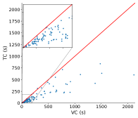
(a) $\operatorname{\textsf{MAZ}}$

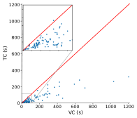
(b) $\operatorname{\textsf{SHB}}$

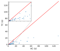
(c) $\operatorname{\textsf{HB}}$

(d) $\operatorname{\textsf{MAZ}}$+Analysis

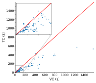
(e) $\operatorname{\textsf{SHB}}$+Analysis

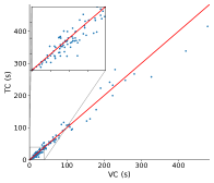
(f) $\operatorname{\textsf{HB}}$+Analysis

Figure 6. Times for processing each benchmark trace using tree clocks (TC) and vector clocks (VC). The top row shows the time for computing the partial order, while the bottom row shows the time including the analysis component.

Setup. Each trace was processed for computing each of the $\operatorname{\textsf{MAZ}}$, $\operatorname{\textsf{SHB}}$ and $\operatorname{\textsf{HB}}$ partial orders using both tree clocks and the standard vector clocks. This allows us to directly measure the speedup conferred by tree clocks in computing the respective partial order, which is the goal of this paper.

As the computation of these partial orders is usually the first component of any analysis, in general, we evaluated the impact of the conferred speedup in an overall analysis as follows. For each pair of conflicting events $e_{1},e_{2}$, we computed whether these events are concurrent wrt the corresponding partial order (e.g., whether $e_{1}\parallel^{\sigma}_{\mathsf{\operatorname{\textsf{HB}}}}e_{2}$). This test is performed in dynamic race detection (in the cases of $\operatorname{\textsf{HB}}$ and $\operatorname{\textsf{SHB}}$) where such pairs constitute data races, as well in stateless model checking (in the case of $\operatorname{\textsf{MAZ}}$) where the model checker identifies such event pairs and attempts to reverse their order on its way to exhaustively enumerate all Mazurkiewicz traces of the concurrent program. For a fair comparison, in the case of $\operatorname{\textsf{HB}}$ we used common epoch optimizations (Flanagan09, ) to speed up the analysis for both tree clocks and vector clocks (recall Remark 1). For consistency, every measurement was repeated 3 times and the average time was reported.

Running times. For each partial order, Table 2 shows the average speedup over all benchmarks, both with and without the analysis component. We see that tree clocks are very effective in reducing the running time of the computation of all 3 partial orders, with the most significant impact being on $\operatorname{\textsf{SHB}}$ where the average speedup is 2.53 times. For the cases of $\operatorname{\textsf{MAZ}}$ and $\operatorname{\textsf{SHB}}$, this speedup also lead to a significant speedup in the overall analysis time. On the other hand, although $\operatorname{\textsf{HB}}$ with tree clocks is about 2 times faster than with vector clocks, this speedup has a smaller effect on the overall analysis time. The reason behind this observation is straightforward: $\operatorname{\textsf{SHB}}$ and $\operatorname{\textsf{MAZ}}$ are much more computationally-heavy, as they are defined using all types of events; on the other hand, $\operatorname{\textsf{HB}}$ is defined only on synchronization events (acq and rel) and on average, only $\simeq 9.5\%$ of the events are synchronization events on our benchmark traces. Since our analysis considers all events, the $\operatorname{\textsf{HB}}$-computation component occupies a smaller fraction of the overall analysis time. We remark, however, that for programs that are more synchronization-heavy, or for analyses that are more lightweight (e.g., when checking for data races on a specific variable as opposed to all variables), the speedup of tree clocks will be larger on the whole analysis. Indeed, Figure 7 shows the obtained speedup on the total analysis time for $\operatorname{\textsf{HB}}$ as a function of synchronization events. We observe a trend for the speedup to increase as the percentage of synchronization events increases in the trace. A further observation is that speedup is prominent when the number of threads are large.

	$\operatorname{\textsf{MAZ}}$	$\operatorname{\textsf{SHB}}$	$\operatorname{\textsf{HB}}$
PO	2.02	2.66	2.97
PO + Analysis	1.49	1.80	1.11

Table 2. Average speedup for computing the partial order due to tree clocks.

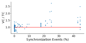
Figure 7. Speedup on $\operatorname{\textsf{HB}}$+analysis computation as a function of the percentage of synchronization events, for the traces where the total time is not too small ($\geq 100$ms).

Figure 6 gives a more detailed view of the tree clocks vs vector clocks times across all benchmarks. We see that tree clocks almost always outperform vector clocks on all partial orders, and in some cases by large margins. Interestingly, the speedup tends to be larger on more demanding benchmarks (i.e., on those that take more time). In the very few cases tree clocks are slower, this is only by a small factor. These are traces where the sub-linear updates of tree clocks only yield a small potential for improvement, which does not justify the overhead of maintaining the more complex tree data structure (as opposed to a vector). Nevertheless, overall tree clocks consistently deliver a generous speedup to each of $\operatorname{\textsf{MAZ}}$, $\operatorname{\textsf{HB}}$ and $\operatorname{\textsf{SHB}}$. Finally, we remark that all these speedups come directly from just replacing the underlying data structure, without any attempt to optimize the algorithm that computes the respective partial order, or its interaction with the data structure.

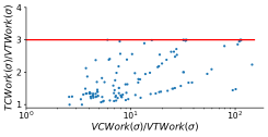
Figure 8. Comparison of the ratios $\operatorname{TCWork}(\sigma)/\operatorname{VTWork}(\sigma)$ and $\operatorname{VCWork}(\sigma)/\operatorname{VTWork}(\sigma)$ across all benchmarks.

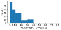
(a) $\operatorname{\textsf{MAZ}}$

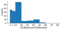
(b) $\operatorname{\textsf{SHB}}$

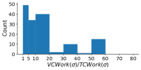
(c) $\operatorname{\textsf{HB}}$

Figure 9. Histogram of the ratios $\operatorname{VCWork}(\sigma)/\operatorname{TCWork}(\sigma)$ across all benchmarks in our dataset.

Comparison with vt-work. We also investigate the total number of entries updated using each of the data structures. Recall that the metric $\operatorname{VTWork}(\sigma)$ (Section 4) measures the minimum amount of updates that any implementation of the vector time must perform when computing the $\operatorname{\textsf{HB}}$ partial order. We can likewise define the metrics $\operatorname{TCWork}(\sigma)$ and $\operatorname{VCWork}(\sigma)$ corresponding to the number of entries updated when processing each event when using respectively the data structures tree clocks and vector clocks. These metrics are visualized in Figure 8 for computing the $\operatorname{\textsf{HB}}$ partial order in our benchmark suite. The figure shows that the $\operatorname{VCWork}(\sigma)/\operatorname{VTWork}(\sigma)$ ratio is often considerably large. In contrast, the ratio $\operatorname{TCWork}(\sigma)/\operatorname{VTWork}(\sigma)$ is typically significantly smaller. The differences in running times between vector and tree clocks reflect the discrepancies between $\operatorname{TCWork}(\cdot)$ and $\operatorname{VCWork}(\cdot)$. Next, recall the intuition behind the optimality of tree clocks (Theorem 4), namely that $\operatorname{TCWork}(\sigma)\leq 3\cdot\operatorname{VTWork}(\sigma)$. Figure 8 confirms this theoretical bound, as the $\operatorname{TCWork}(\sigma)/\operatorname{VTWork}\allowbreak(\sigma)$ ratio stays nicely upper-bounded by $3$ while the $\operatorname{VCWork}(\sigma)/\allowbreak\operatorname{VTWork}(\sigma)$ ratio grows to nearly $100$. Interestingly, for some benchmarks we have $\operatorname{TCWork}(\sigma)\simeq 2.99\cdot\operatorname{VTWork}(\sigma)$, i.e., these benchmarks push tree clocks to their vt-work upper-bound. Going one step further, Figure 9 shows the ratio $\operatorname{VCWork}(\sigma)/\operatorname{TCWork}(\sigma)$ for each partial order in our dataset. The results indicate that vector clocks perform a lot of unnecessary work compared to tree clocks, and experimentally demonstrate the source of speedup on tree clocks. Although Figure 9 indicates that the potential for speedup can be large (reaching $55\times$), the actual speedup in our experiments (Figure 6) is smaller, as a single tree clock operation is more computationally heavy than a single vector clock operation.

Scalability. To get a better insight on the scalability of tree clocks, we performed a set of controlled experiments on custom benchmarks, by controlling the number of threads and the number of locks parameters while keeping the communication patterns constant. Each trace consists of $10$M events, while the number of threads varies between $10$ and $360$. The traces are generated in a way such that a randomly chosen thread performs two consecutive operations, $acq(l)$ followed by a $rel(l)$, on a randomly (when applicable) chosen lock $l$. We have considered four cases: (a) all threads communicate over a single common lock (single lock); (b) similar to (a), but there are 50 locks, and $20\%$ of the threads are $5$ times more likely to perform an operation compared to the rest of the threads (50 locks, skewed); (c) $k-1$ client threads communicate with a single server thread via a dedicated lock per thread (star topology); (d) similar to (a), but every pair of threads communicates over a dedicated lock (pairwise communication).

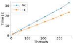
(a) Single lock

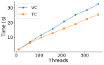
(b) Fifty locks

(c) Star topology

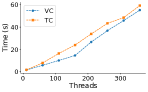
(d) Pairwise communication

Figure 10. Comparison of tree clocks (TC) and vector clocks (VC) on $4$ different benchmarks with increasing number of threads.

Figure 10 shows the obtained results. Scenario (a) shows how tree clocks have a constant-factor speedup over vector clocks in this setting. As we move to more locks in scenario (b), thread communication becomes more independent and the benefit of tree clocks may slightly diminish. As a subset of the threads is more active than the rest, timestamps are frequently exchanged through them, making tree clocks faster in this setting as well. Scenario (c) represents a case in which tree clocks thrive: while the time taken by vector clocks increases with the number of threads, it stays constant for tree clocks. This is because the star topology implies that, on average, every tree clock join and copy operation only affects a constant number of tree clock entries, despite the fact that every thread is aware of the state of every other thread. Intuitively, the star communication topology naturally affects the shape of the tree to (almost) a star, which leads to this effect. Finally, scenario (d) represents the worst case for tree clocks as all pairs of threads can communicate with each other and the communication is conducted via a unique lock per thread pair. This pattern nullifies the benefit of tree clocks, while their increased complexity results in a general slowdown. However, even in this worst-case scenario, the difference between tree clocks and vector clocks remains relatively small.

7. Related Work

Other partial orders and tree clocks. As we have mentioned in the introduction, besides $\operatorname{\textsf{HB}}$ and $\operatorname{\textsf{SHB}}$, many other partial orders perform dynamic analysis using vector clocks. In such cases, tree clocks can replace vector clocks either partially or completely, sometimes requiring small extensions to the data structure as presented here. In particular, we foresee interesting applications of tree clocks for the $\operatorname{\textsf{WCP}}$ (Kini17, ), $\operatorname{\textsf{DC}}$ (Roemer18, ) and $\operatorname{\textsf{SDP}}$ (Genc19, ) partial orders.

Speeding up dynamic analyses. Vector-clock based dynamic race detection is known to be slow (sadowski-tools-2014, ), which many prior works have aimed to mitigate. One of the most prominent performance bottlenecks is the linear dependence of the size of vector timestamps on the number of threads. Despite theoretical limits (CharronBost1991, ), prior research exploits special structures in traces (cheng1998detecting, ; Feng1997, ; surendran2016dynamic, ; Dimitrov2015, ; Agrawal2018, ) that enable succinct vector time representations. The Goldilocks (Elmas07, ) algorithm infers $\operatorname{\textsf{HB}}$-orderings using locksets instead of vector timestamps but incurs severe slowdown (Flanagan09, ). The FastTrack (Flanagan09, ) optimization uses epochs for maintaining succinct access histories and our work complements this optimization — tree clocks offer optimizations for other clocks (thread and lock clocks). Other optimizations in clock representations are catered towards dynamic thread creation (Raychev2013, ; Wang2006, ; Raman2012, ). Another major source of slowdown is program instrumentation and expensive metadata synchronization. Several approaches have attempted to minimize this slowdown, including hardware assistance (RADISH2012, ; HARD2007, ), hybrid race detection (OCallahan03, ; Yu05, ), static analysis (bigfoot2017, ; redcard2013, ), and sophisticated ownership protocols (Bond2013, ; Wood2017, ; Roemer20, ).

8. Conclusion

We have introduced tree clocks, a new data structure for maintaining logical times in concurrent executions. In contrast to standard vector clocks, tree clocks can dynamically capture communication patterns in their structure and perform join and copy operations in sublinear time, thereby avoiding the traditional overhead of these operations when possible. Moreover, we have shown that tree clocks are vector-time optimal for computing the $\operatorname{\textsf{HB}}$ partial order, performing at most a constant factor work compared to what is absolutely necessary, in contrast to vector clocks. Finally, our experiments show that tree clocks effectively reduce the running time for computing the $\operatorname{\textsf{MAZ}}$, $\operatorname{\textsf{SHB}}$ and $\operatorname{\textsf{HB}}$ partial orders significantly, and thus offer a promising alternative over vector clocks.

Interesting future work includes incorporating tree clocks in an online analysis such as ThreadSanitizer (threadsanitizer, ). Any use of additional synchronization to maintain analysis atomicity in this online setting is identical and of the same granularity to both vector clocks and tree clocks. However, the faster joins performed by tree clocks may lead to less congestion compared to vector clocks, especially for partial orders such as $\operatorname{\textsf{SHB}}$ and $\operatorname{\textsf{MAZ}}$ where synchronization occurs on all events (i.e., synchronization, as well as access events). We leave this evaluation for future work. Finally, since tree clocks are a drop-in replacement of vector clocks, most of the existing techniques that minimize the slowdown due to metadata synchronization (Section 7) are directly applicable to tree clocks.

Appendix A Proofs

See 1

Proof.

Consider a trace $\sigma$, a release event $\texttt{rel}(\ell)$ and let $\texttt{acq}(\ell)$ be the matching acquire event. When $\texttt{acq}(\ell)$ is processed the algorithm performs $\mathbb{C}_{t}\leftarrow\mathbb{C}_{t}\sqcup\mathbb{C}_{\ell}$, and thus $\mathbb{C}_{\ell}\sqsubseteq\mathbb{C}_{t}$ after this operation. By lock semantics, there exists no release event $\texttt{rel}^{\prime}(\ell)$ such that $\texttt{acq}(\ell)<^{\sigma}\texttt{rel}^{\prime}(\ell)<^{\sigma}\texttt{rel}(\ell)$, and hence $\mathbb{C}_{\ell}$ is not modified until $\texttt{rel}(\ell)$ is processed. Since vector clock entries are never decremented, when $\texttt{rel}(\ell)$ is processed we have $\mathbb{C}_{\ell}\sqsubseteq\mathbb{C}_{t}$, as desired. ∎

See 2

Proof.

First, note that after initialization $u$ has no children, hence each statement is trivially true. Now assume that both statements hold when the algorithm processes an event $e$, and we show that they both hold after the algorithm has processed $e$. We distinguish cases based on the type of $e$.

$e=\langle t,\texttt{acq}(\ell)\rangle$. The algorithm performs the operation $\mathbb{C}_{t}.\textnormal{{Join}}(\mathbb{L}_{\ell})$, hence the only tree clock modified is $\mathbb{C}_{t}$, and thus it suffices to examine the cases that $\mathbb{C}_{t}$ is $\mathbb{C}$ and $\mathbb{C}_{t}$ is $\mathbb{C}^{\prime}$.

1. $\mathbb{C}_{t}$ is $\mathbb{C}$. First consider the case that $u=\mathbb{C}_{t}.\operatorname{T}.\operatorname{root}$. Observe that $u.\operatorname{clk}>\mathbb{C}^{\prime}.\textnormal{{Get}}(u.\operatorname{\mathsf{tid}})$, and thus Item 1. holds trivially. For Item 2., we distinguish cases based on whether $v.\operatorname{clk}$ has progressed by the Join operation. If yes, then we have $v.\operatorname{aclk}=u.\operatorname{clk}$, and the statement holds trivially for the same reason as in Item 1.. Otherwise, we have that for every descendant $w$ of $v$, the clock $w.\operatorname{clk}$ has not progressed by the Join operation, hence the statement holds by the induction hypothesis on $\mathbb{C}_{t}$.

   Now consider the case that $u\neq\mathbb{C}_{t}.\operatorname{T}.\operatorname{root}$. If $u.\operatorname{clk}$ has not progressed by the Join operation then each statement holds by the induction hypothesis on $\mathbb{C}_{t}$. Otherwise, using the induction hypothesis one can show that for every descendant $w$ of $u$, there exists a node $w_{\ell}$ of $\mathbb{L}_{\ell}$ that is a descendant of a node $u_{\ell}$ such that $w_{\ell}.\operatorname{\mathsf{tid}}=w.\operatorname{\mathsf{tid}}$ and $u_{\ell}.\operatorname{\mathsf{tid}}=u.\operatorname{\mathsf{tid}}$. Then, each statement holds by the induction hypothesis on $\mathbb{L}_{\ell}$.

2. $\mathbb{C}_{t}$ is $\mathbb{C}^{\prime}$. For Item 1., if $u.\operatorname{clk}\leq\mathbb{C}^{\prime}.\textnormal{{Get}}(u.\operatorname{\mathsf{tid}})$ holds before the Join operation, then the statement holds by the induction hypothesis, since Join does not decrease the clocks of $\mathbb{C}_{t}$. Otherwise, the statement follows by the induction hypothesis on $\mathbb{L}_{\ell}$. The analysis for Item 2. is similar.

   The desired result follows.

$e=\langle t,\texttt{rel}(\ell)\rangle$. The algorithm performs the operation $\mathbb{L}_{\ell}.\linebreak\textnormal{{MonotoneCopy}}(\mathbb{C}_{t})$. The analysis is similar to the previous case, this time also using Lemma 1 to argue that no time stored in $\mathbb{L}_{\ell}$ decreases. ∎

See 3

Proof.

The lemma follows directly from Lemma 2. In each case, if the corresponding operation (i.e., Join for event $\langle t,\texttt{acq}(\ell)\rangle$ and MonotoneCopy for $\langle t,\texttt{rel}(\ell)\rangle$), if the clock of a node $w$ of the tree clock that performs the operation does not progress, then we are guaranteed that $w.\operatorname{clk}$ is not smaller than the time of the thread $w.\operatorname{\mathsf{tid}}$ in the tree clock that is passed as an argument to the operation. ∎

First remote acquires. Consider a trace $\sigma$ and a lock-release event $e=\langle t,\texttt{rel}(\ell)\rangle$ of $\sigma$, such that there exists a later acquire event $e^{\prime}=\langle t^{\prime},\texttt{acq}(\ell)\rangle$ ($e<^{\sigma}_{\mathsf{\operatorname{\textsf{tr}}}}e^{\prime}$). The first remote acquire of $e$ is the first event $e^{\prime}$ with the above property. For example, in Figure 11(a), $e_{7}$ is the first remote acquire of $e_{2}$. While constructing the $\operatorname{\textsf{HB}}$ partial order, the algorithm makes $\operatorname{\textsf{HB}}$ orderings from lock-release events to their first remote acquires $\texttt{rel}(\ell)<^{\sigma}_{\mathsf{\operatorname{\textsf{HB}}}}\texttt{acq}(\ell)$. The following lemma captures the property that the edges of tree clocks are essentially the inverses of such orderings.

Lemma 0.

Consider the execution of Algorithm 3 on a trace $\sigma$. For every tree clock $\mathbb{C}_{i}$ and node $u$ of $\mathbb{C}_{i}.\operatorname{T}$ other than the root, the following assertions hold.

1. $u$ points to a lock-release event $\texttt{rel}(\ell)$.

2. $\texttt{rel}(\ell)$ has a first remote acquire $\texttt{acq}(\ell)$ and $(v.\operatorname{\mathsf{tid}},u.\operatorname{aclk})$ points to $\texttt{acq}(\ell)$, where $v$ is the parent of $u$ in $\mathbb{C}_{i}.\operatorname{T}$.

Proof.

The lemma follows by a straightforward induction on $\sigma$. ∎

Lemma 1 allows us to prove the vt-optimality of tree clocks.

See 4

Proof.

Consider a critical section of a thread $t$ on lock $\ell$, marked by two events $\texttt{acq}(\ell)$, $\texttt{rel}(\ell)$. We define the following vector times.

1. $\operatorname{V}_{t}^{1}$ and $\operatorname{V}_{t}^{2}$ are the vector times of $\mathbb{C}_{t}$ right before and right after $\texttt{acq}(\ell)$ is processed, respectively.

2. $\operatorname{V}_{\ell}^{1}$ is the vector time of $\mathbb{C}_{\ell}$ right before $\texttt{acq}(\ell)$ is processed.

3. $\operatorname{V}_{t}^{3}$ is the vector time of $\mathbb{C}_{t}$ right before $\texttt{rel}(\ell)$ is processed.

4. $\operatorname{V}_{\ell}^{3}$ and $\operatorname{V}_{\ell}^{4}$ are the vector times of $\mathbb{C}_{\ell}$ right before and right after $\texttt{rel}(\ell)$ is processed, respectively,

First, note that (i) $\operatorname{V}_{t}^{1}\sqsubseteq\operatorname{V}_{t}^{3}$, and (ii) due to lock semantics, we have $\operatorname{V}_{\ell}^{3}=\operatorname{V}_{\ell}^{1}$. Let $W=W_{J}+W_{C}$, where

$$W_{J}= |\{t^{\prime}\colon\operatorname{V}_{t}^{2}(t^{\prime})\neq\operatorname{V}_{t}^{1}(t^{\prime})\}|\quad\text{ and}$$

$$W_{C}= |\{t^{\prime}\colon\operatorname{V}_{\ell}^{4}(t^{\prime})\neq\operatorname{V}_{\ell}^{3}(t^{\prime})\}|$$

i.e., $W_{J}$ and $W_{C}$ are the vt-work for handling $\texttt{acq}(\ell)$ and $\texttt{rel}(\ell)$, respectively. Let $\mathcal{T}_{J}$ be the time spent in $\operatorname{TC}_{t}.\textnormal{{Join}}$ due to $\texttt{acq}(\ell)$. Similarly, let $\mathcal{T}_{C}$ be the time spent in $\operatorname{TC}_{\ell}.\textnormal{{MonotoneCopy}}$ due to $\texttt{rel}(\ell)$. We will argue that $\mathcal{T}_{J}=O(W)$ and $\mathcal{T}_{C}=O(W_{C})$, and thus $\mathcal{T}_{J}+\mathcal{T}_{C}=O(W)$. Note that this proves the lemma, simply by summing over all critical sections of $\sigma$.

We start with $\mathcal{T}_{J}$. Observe that the time spent in this operation is proportional to the number of times the loop in Algorithm 2 is executed, i.e., the number of nodes $v^{\prime}$ that the loop iterates over. Consider the if statement in Algorithm 2. If $\textnormal{{Get}}(v^{\prime}.\operatorname{\mathsf{tid}})<v^{\prime}.\operatorname{clk}$, then we have $\operatorname{V}_{t}^{2}(v^{\prime}.\operatorname{\mathsf{tid}})>\operatorname{V}_{t}^{1}(v^{\prime}.\operatorname{\mathsf{tid}})$, and thus this iteration is accounted for in $W_{J}$. On the other hand, if $\textnormal{{Get}}(v^{\prime}.\operatorname{\mathsf{tid}})>v^{\prime}.\operatorname{clk}$, then we have $\operatorname{V}_{t}^{1}(v^{\prime}.\operatorname{\mathsf{tid}})>\operatorname{V}_{\ell}^{1})(v^{\prime}.\operatorname{\mathsf{tid}})$. Due to (i) and (ii) above, we have $\operatorname{V}_{\ell}^{4}(v^{\prime}.\operatorname{\mathsf{tid}})>\operatorname{V}_{\ell}^{3}(v^{\prime}.\operatorname{\mathsf{tid}})$, and thus this iteration is accounted for in $W_{C}$. Finally, consider the case that $\textnormal{{Get}}(v^{\prime}.\operatorname{\mathsf{tid}})=v^{\prime}.\operatorname{clk}$, and let $v$ be the node of $\mathbb{C}_{t}$ such that $v.\operatorname{\mathsf{tid}}=v^{\prime}.\operatorname{\mathsf{tid}}$. There can be at most one such $v$ that is not the root of $\operatorname{TC}_{t}$. For every other such $v$, let $u=\operatorname{Prnt}(v)$. Note that $v^{\prime}$ is not the root of $\mathbb{C}_{\ell}$, and let $u^{\prime}=\operatorname{Prnt}(v^{\prime})$. Let $\texttt{rel}(\ell)$ be the lock-release event that $v$ and $v^{\prime}$ point to. By Lemma 1, $\texttt{rel}(\ell)$ has a first remote acquire $\texttt{acq}(\ell)$ such that (i) $u.\operatorname{\mathsf{tid}}=u^{\prime}.\operatorname{\mathsf{tid}}=t^{\prime}$, where $t^{\prime}$ is the thread of $\texttt{acq}(\ell)$, and (ii) $v.\operatorname{aclk}$ is the local clock of $\texttt{acq}(\ell)$. Since getUpdatedNodesCopy examines $v^{\prime}$, we must have $u^{\prime}.\operatorname{clk}>u.\operatorname{clk}$. In turn, we have $u.\operatorname{clk}\geq v.\operatorname{aclk}$, and thus $u^{\prime}.\operatorname{aclk}>v.\operatorname{aclk}$. Hence, due to Algorithm 2, $u^{\prime}$ can have at most one child $v^{\prime}$ with $v^{\prime}.\operatorname{clk}=\textnormal{{Get}}(v^{\prime}.\operatorname{\mathsf{tid}})$. Thus, we can account for the time of this case in $W_{J}$. Hence, $\mathcal{T}_{J}=O(W)$, as desired.

We now turn our attention to $\mathcal{T}_{C}$. Similarly to the previous case, the time spent in this operation is proportional to the number of times the loop in Algorithm 2 is executed. Consider the if statement in Algorithm 2. If $\textnormal{{Get}}(v^{\prime}.\operatorname{\mathsf{tid}})<v^{\prime}.\operatorname{clk}$, then we have $\operatorname{V}_{\ell}^{4}(v^{\prime}.\operatorname{\mathsf{tid}})>\operatorname{V}_{\ell}^{3}(v^{\prime}.\operatorname{\mathsf{tid}})$, and thus this iteration is accounted for in $W_{C}$. Note that as the copy is monotone (Lemma 1), we can’t have $\textnormal{{Get}}(v^{\prime}.\operatorname{\mathsf{tid}})>v^{\prime}.\operatorname{clk}$. Finally, the reasoning for the case where $\textnormal{{Get}}(v^{\prime}.\operatorname{\mathsf{tid}})=v^{\prime}.\operatorname{clk}$ is similar to the analysis of $\mathcal{T}_{J}$, using Algorithm 2 instead of Algorithm 2. Hence, $\mathcal{T}_{C}=O(W_{C})$, as desired.

The desired result follows. ∎

Appendix B Example of Tree Clocks in $\operatorname{\textsf{HB}}$

(a) An example trace $\sigma$.

(b) The sequence of tree-clock updates after $\operatorname{\textsf{HB}}$ processes each event $e_{i}$ of $\sigma$. Only the tree clock $\operatorname{TC}_{j}$ of thread $j$ that performs $e_{i}$ is shown. When the thread performs a lock-release the corresponding tree clock of the lock is mentioned in parenthesis.

Figure 11. Example run of $\operatorname{\textsf{HB}}$ and the updates on the corresponding clock-trees.

Figure 11 shows an example run of Algorithm 3 on a trace $\sigma$, showing how tree clocks grow during the execution. The figure shows the tree clocks $\mathbb{C}_{t}$ of the threads; the tree clocks of locks $\mathbb{C}_{\ell}$ are just copies of the former after processing a lock-release event (shown in parentheses in the figure). Figure 12 presents a closer look of the Join and MonotoneCopy operations for the last events of $\sigma$.

(a) Details of the join operation due to $e_{15}$. $\operatorname{TC}_{{\color[rgb]{0.24,0.24,0.24}\ell_{2}}}$ shows the tree clock of lock $\ell_{2}$. $\operatorname{TC}_{2}$ shows the tree clock of thread $t_{2}$ right before performing the operation $\operatorname{TC}_{2}.\textnormal{{Join}}(\operatorname{TC}_{{\color[rgb]{0.24,0.24,0.24}\ell_{2}}})$. Note that $\operatorname{TC}_{2}$ is not yet aware of thread $t_{4}$. The result is $\operatorname{TC}_{2}$ shown in Figure 11(b).

(b) Details of processing $e_{16}$. $\operatorname{TC}_{2}$ shows the tree clock of thread $t_{2}$. $\operatorname{TC}_{{\color[rgb]{0.24,0.24,0.24}\ell_{2}}}$ shows the tree clock of lock $\ell_{2}$ right before performing $\operatorname{TC}_{{\color[rgb]{0.24,0.24,0.24}\ell_{2}}}.\textnormal{{MonotoneCopy}}(\operatorname{TC}_{2})$. Note that $\operatorname{TC}_{{\color[rgb]{0.24,0.24,0.24}\ell_{2}}}$ is not yet aware of thread $t_{2}$. The result is $\operatorname{TC}_{{\color[rgb]{0.24,0.24,0.24}\ell_{2}}}$ shown in Figure 11(b).

Figure 12. A closer look at the last two steps of the example of Figure 11 in the processing of events $e_{15}$ and $e_{16}$. In each figure, light gray marks the nodes of the left tree clock whose vector time is compared to the time of the tree clock on the right. Similarly, dark gray marks the nodes of the left (resp., right) tree clock that are updating (resp., being updated).

Appendix C Benchmarks

Information on Benchmark Traces. We denote by $\mathcal{N}$, $\mathcal{T}$, $\mathcal{M}$ and $\mathcal{L}$ the total number of events, number of threads, number of memory locations and number of locks, respectively.

Benchmark $\mathcal{N}$ $\mathcal{T}$ $\mathcal{M}$ $\mathcal{L}$

Benchmark $\mathcal{N}$ $\mathcal{T}$ $\mathcal{M}$ $\mathcal{L}$

[h*]rcccc CoMD-omp-task-1 & 175.1M 56 66.1K 114
CoMD-omp-task-2 175.1M 56 66.1K 114
CoMD-omp-task-deps-1 174.1M 16 63.0K 34
CoMD-omp-task-deps-2 175.1M 56 66.1K 114
CoMD-omp-taskloop-1 251.5M 16 4.0M 35
CoMD-omp-taskloop-2 251.5M 56 4.0M 115
CoMD-openmp-1 174.1M 16 63.0K 34
CoMD-openmp-2 175.1M 56 66.1K 114
DRACC-OMP-009-Counter-wrong-critical-yes 135.0M 16 971 36
DRACC-OMP-010-Counter-wrong-critical-Intra-yes 135.0M 16 971 36
DRACC-OMP-011-Counter-wrong-critical-Inter-yes 135.0M 16 853 21
DRACC-OMP-012-Counter-wrong-critical-simd-yes 104.9M 16 1.5K 36
DRACC-OMP-013-Counter-wrong-critical-simd-Intra-yes 104.9M 16 1.5K 36
DRACC-OMP-014-Counter-wrong-critical-simd-Inter-yes 104.9M 16 1.4K 21
DRACC-OMP-015-Counter-wrong-lock-yes 135.0M 16 971 36
DRACC-OMP-016-Counter-wrong-lock-Intra-yes 135.0M 16 971 36
DRACC-OMP-017-Counter-wrong-lock-Inter-yes-1 135.0M 16 853 21
DRACC-OMP-017-Counter-wrong-lock-Inter-yes-2 27.0M 16 853 21
DRACC-OMP-018-Counter-wrong-lock-simd-yes 104.9M 16 1.5K 36
DRACC-OMP-019-Counter-wrong-lock-simd-Intra-yes 104.9M 16 1.5K 36
DRACC-OMP-020-Counter-wrong-lock-simd-Inter-yes 104.9M 16 1.4K 21
DataRaceBench-DRB062-matrixvector2-orig-no-1 183.9M 16 7.0K 33
DataRaceBench-DRB062-matrixvector2-orig-no-2 193.2M 56 9.0K 113
DataRaceBench-DRB105-taskwait-orig-no-1 134.0M 16 3.2K 33
DataRaceBench-DRB105-taskwait-orig-no-2 134.0M 56 9.7K 113
DataRaceBench-DRB106-taskwaitmissing-orig-yes-1 134.0M 16 3.6K 33
DataRaceBench-DRB106-taskwaitmissing-orig-yes-2 134.0M 56 11.0K 113
DataRaceBench-DRB110-ordered-orig-no-1 120.0M 16 775 36
DataRaceBench-DRB110-ordered-orig-no-2 120.0M 56 2.3K 116
DataRaceBench-DRB122-taskundeferred-orig-no-1 112.0M 16 956 33
DataRaceBench-DRB122-taskundeferred-orig-no-2 112.0M 56 3.0K 113
DataRaceBench-DRB123-taskundeferred-orig-yes-1 112.0M 16 1.2K 33
DataRaceBench-DRB123-taskundeferred-orig-yes-2 112.0M 56 3.7K 113
DataRaceBench-DRB144-critical-missingreduction-orig-gpu-yes 140.0M 16 966 35
DataRaceBench-DRB148-critical1-orig-gpu-yes 135.0M 16 971 36
DataRaceBench-DRB150-missinglock1-orig-gpu-yes 112.0M 16 968 35
DataRaceBench-DRB152-missinglock2-orig-gpu-no 112.0M 16 968 35
DataRaceBench-DRB154-missinglock3-orig-gpu-no.c 112.0M 16 851 20
DataRaceBench-DRB155-missingordered-orig-gpu-no-1 50.0M 16 2.0M 36
DataRaceBench-DRB155-missingordered-orig-gpu-no-2 50.0M 56 2.0M 116
DataRaceBench-DRB176-fib-taskdep-no-1 1.6B 17 12.4K 33
DataRaceBench-DRB176-fib-taskdep-no-2 1.6B 57 41.3K 113
DataRaceBench-DRB176-fib-taskdep-no-3 618.3M 17 11.7K 33
DataRaceBench-DRB176-fib-taskdep-no-4 618.3M 57 38.3K 113
DataRaceBench-DRB176-fib-taskdep-no-5 90.2M 17 9.8K 33
DataRaceBench-DRB176-fib-taskdep-no-6 90.3M 57 30.9K 113
DataRaceBench-DRB177-fib-taskdep-yes-1 1.6B 17 10.5K 33
DataRaceBench-DRB177-fib-taskdep-yes-2 382.1M 17 9.3K 33
DataRaceBench-DRB177-fib-taskdep-yes-3 236.2M 17 9.0K 33
DataRaceBench-DRB177-fib-taskdep-yes-4 1.0B 17 10.0K 33
DataRaceBench-DRB177-fib-taskdep-yes-5 618.3M 17 9.8K 33
DataRaceBench-DRB177-fib-taskdep-yes-6 618.3M 57 30.6K 113
DataRaceBench-DRB177-fib-taskdep-yes-7 90.2M 17 8.7K 33
DataRaceBench-DRB177-fib-taskdep-yes-8 90.3M 57 25.5K 113
OmpSCR-v2.0-c-LUreduction-1 136.4M 16 181.6K 34
OmpSCR-v2.0-c-LUreduction-2 136.9M 56 183.6K 114
OmpSCR-v2.0-c-Mandelbrot-1 115.7M 16 3.0K 34
OmpSCR-v2.0-c-Mandelbrot-2 115.7M 56 5.1K 114
OmpSCR-v2.0-c-MolecularDynamic-1 204.3M 16 7.2K 34
OmpSCR-v2.0-c-MolecularDynamic-2 204.4M 56 9.4K 114
OmpSCR-v2.0-c-Pi-1 150.0M 16 976 34
OmpSCR-v2.0-c-Pi-2 150.0M 56 3.0K 114
OmpSCR-v2.0-c-QuickSort-1 134.3M 16 101.6K 35
OmpSCR-v2.0-c-QuickSort-2 134.3M 56 103.6K 115
OmpSCR-v2.0-c-fft-2 2.1B 57 29.4M 115
OmpSCR-v2.0-c-fft-3 496.0M 17 7.3M 35
OmpSCR-v2.0-c-fft-4 496.0M 57 7.3M 115
OmpSCR-v2.0-c-fft6-1 146.0M 16 4.3M 49
OmpSCR-v2.0-c-fft6-2 146.0M 56 5.3M 132
OmpSCR-v2.0-c-testPath-1 30.2M 16 2.8M 35
OmpSCR-v2.0-c-testPath-2 37.5M 56 2.8M 115
OmpSCR-v2.0-c-LoopsWithDependencies-c-loopA.badSolution-1 112.6M 16 161.0K 34
OmpSCR-v2.0-c-LoopsWithDependencies-c-loopA.badSolution-2 394.0M 56 563.0K 114
OmpSCR-v2.0-c-LoopsWithDependencies-c-loopA.solution1-1 192.6M 16 321.0K 34
OmpSCR-v2.0-c-LoopsWithDependencies-c-loopA.solution1-2 674.2M 56 1.1M 114
OmpSCR-v2.0-c-LoopsWithDependencies-c-loopA.solution2-1 337.2M 56 562.7K 114
OmpSCR-v2.0-c-LoopsWithDependencies-c-loopA.solution2-2 96.4M 16 160.9K 34
OmpSCR-v2.0-c-LoopsWithDependencies-c-loopA.solution3-1 337.3M 56 562.7K 114
OmpSCR-v2.0-c-LoopsWithDependencies-c-loopA.solution3-2 96.4M 16 160.9K 34
OmpSCR-v2.0-c-LoopsWithDependencies-c-loopB.badSolution1-1 112.6M 16 161.0K 34
OmpSCR-v2.0-c-LoopsWithDependencies-c-loopB.badSolution1-2 394.0M 56 563.0K 114
OmpSCR-v2.0-cpp-sortOpenMP-cpp-qsomp1-1 107.0M 16 101.2K 35
OmpSCR-v2.0-cpp-sortOpenMP-cpp-qsomp1-2 106.8M 56 103.5K 115
OmpSCR-v2.0-cpp-sortOpenMP-cpp-qsomp2-1 107.1M 56 104.7K 115
OmpSCR-v2.0-cpp-sortOpenMP-cpp-qsomp2-2 107.5M 16 101.5K 35
OmpSCR-v2.0-cpp-sortOpenMP-cpp-qsomp3-1 115.4M 56 10.0M 115
OmpSCR-v2.0-cpp-sortOpenMP-cpp-qsomp3-2 141.7M 16 10.0M 35
OmpSCR-v2.0-cpp-sortOpenMP-cpp-qsomp4-1 114.2M 56 104.7K 115
OmpSCR-v2.0-cpp-sortOpenMP-cpp-qsomp4-2 164.0M 16 101.5K 35
OmpSCR-v2.0-cpp-sortOpenMP-cpp-qsomp6 106.7M 56 104.8K 115
OmpSCR-v2.0-cpp-sortOpenMP-cpp-qsomp7-1 295.5M 56 82.9K 114
OmpSCR-v2.0-cpp-sortOpenMP-cpp-qsomp7-2 88.9M 16 31.6K 34
HPCCG-1 228.1M 16 935.9K 34
HPCCG-2 229.5M 56 938.4K 114
graph500-1 171.3M 16 228.8K 34
graph500-2 172.5M 56 233.4K 114
SimpleMOC 170.2M 16 4.3M 5.0K
NPBS-DC.S-1 11.7M 16 3.6M 36
NPBS-DC.S-2 11.7M 56 3.7M 115
NPBS-IS.W-1 152.9M 16 2.2M 34
NPBS-IS.W-2 300.1M 56 2.3M 114
Kripke-1 117.5M 16 203.1K 35
Kripke-2 119.2M 56 205.8K 116
Lulesh-1 35.3M 17 159.5K 33
Lulesh-2 52.1M 56 164.0K 114
Lulesh-3 543.4M 17 1.3M 34
Lulesh-4 569.5M 57 1.2M 114
QuickSilver 132.6M 56 914.1K 116
RSBench-1 1.3B 16 2.0M 34
RSBench-2 1.3B 56 2.0M 114
XSBench-1 96.6M 16 25.7M 33
XSBench-2 96.6M 56 25.7M 114
amg2013-1 169.9M 18 2.8M 74
amg2013-2 189.6M 58 4.5M 154
miniFE-1 206.7M 58 1.2M 154
miniFE-2 207.7M 18 1.2M 74
account 134 5 41 3
airlinetickets 140 5 44 0
array 51 4 30 2
batik 157.9M 7 4.9M 1.9K
boundedbuffer 332 3 63 2
bubblesort 4.6K 13 167 2
bufwriter 22.2K 7 471 1
clean 1.3K 10 26 2
critical 59 5 30 0
cryptorsa 58.5M 9 1.7M 8.0K
derby 1.4M 5 185.6K 1.1K
ftpserver 49.6K 12 5.5K 301
jigsaw 3.1M 12 103.5K 275
lang 6.3K 8 1.5K 0
linkedlist 1.0M 13 3.1K 1.0K
lufact 134.1M 5 252.1K 1
luindex 397.8M 3 2.5M 65
lusearch 217.5M 8 5.2M 118
mergesort 3.0K 6 621 3
moldyn 200.3K 4 1.2K 2
pingpong 151 7 51 0
producerconsumer 658 9 67 3
raytracer 15.8K 4 3.9K 8
readerswriters 11.3K 6 18 1
sor 606.9M 5 1.0M 2
sunflow 11.7M 17 1.3M 9
tsp 307.3M 10 181.1K 2
twostage 193 13 21 2
wronglock 246 23 26 2
xalan 122.5M 7 4.4M 2.5K
biojava 221.0M 4 121.0K 78
cassandra 259.1M 173 9.9M 60.5K
graphchi 215.8M 20 24.9M 60
hsqldb 18.8M 44 945.0K 401
tradebeans 39.1M 222 2.8M 6.1K
tradesoap 39.1M 221 2.8M 6.1K
zxing 546.4M 15 37.8M 1.5K