Multinomial Backtesting of Distortion Risk Measures

Abstract

We extend the scope of risk measures for which backtesting models are available by proposing a multinomial backtesting method for general distortion risk measures. The method relies on a stratification and randomization of risk levels. We illustrate the performance of our methods in numerical case studies.

Keywords:
Distortion Risk Measures, Backtesting, Multinomial Tests, Solvency Capital, Internal Models.

1 Introduction

In the face of risk and uncertainty financial institutions need to measure and quantify the risk they are exposed to. These measurements can be used to determine the capital that is needed as a buffer against adverse scenarios. Risk measures also help to compare portfolios or balance sheets to each other and to guide management decisions. In this paper, we extend the scope of risk measures for which backtesting models are available.

A variety of risk measures has been suggested in the literature. Value at Risk (V@R) and Average Value at Risk (AV@R) are the basis of different solvency regimes. An axiomatic investigation of monetary risk measures goes back to Artzner et al. (1999), Föllmer and Schied (2002), and Frittelli and Gianin (2002), see also Föllmer and Schied (2016) and Föllmer and Weber (2015). We introduce a general methodology for backtesting an important class of risk measures that includes the regulatory benchmarks V@R and AV@R as special cases: distortion risk measures (DRMs).

DRMs encompass all distribution-based coherent risk measures. This fact is a direct consequence of a representation theorem by Kusuoka (2001). But DRMs include many additional risk measures that are not necessarily convex, e.g. V@R and Range Value at Risk (RV@R). DRMs are important examples of comonotonic risk measures, i.e., risk measures for which risks simply add up for comonotonic positions.

In practice, risk measures are used to assess the risk of future positions and balance sheets. They are applied to probabilistic models that are estimated from past data. Backtesting refers to methodologies that compare observed values of positions to model-based risk assessments. The methods test the adequacy of the risk measurement models of banks and insurance companies in the face of uncertainty and help to identify misspecifications that impair risk assessments. Thereby financial firms can validate their forecasting tools for investments and balance sheets positions on both the asset and liability side.

It is extremely important that risk measures adequately capture those properties that are needed in the risk management process. Risk measures quantify risk. By numerically representing risk, they facilitate the communication within firms, with customers, investors and regulators and provides a solid basis for decisions. Risk measures reduce the complexity of risk by focussing on specific features of random positions. These issues are systematically studied in the axiomatic theory of risk measures that also provides a variety of examples with different properties, cf. Föllmer and Schied (2016) and Föllmer and Weber (2015). In this paper, we complement this literature by expanding the class of risk measures for which powerful backtesting algorithms are available.

Our contributions are the following:

1. We propose a multinomial backtesting method for general DRMs which extends the non-randomized AV@R-backtest of Kratz et al. (2018). The method relies on a stratification and randomization of risk levels. Our stratified mixture approach captures important characteristics of the DRM by weighting quantiles according to their contribution.

2. We illustrate the performance of our methods in numerical case studies. First, we consider fixed distributions of loss positions under the null hypothesis and under the alternatives and evaluate the size and the power of our test in this simple setting. Second, we apply our method to asset-liability-management.

3. In the special case of AV@R, our backtesting methodology deviates from previously considered multinomial backtests suggested in Kratz et al. (2018) due to the randomization of risk levels. A numerical comparison of both methods shows that our approach improves the power of the backtests in all case studies.

Literature

For reviews on the theory of monetary risk measures, including distortion risk measures, we refer to Föllmer and Schied (2016) and Föllmer and Weber (2015). References to various seminal papers, including Value at Risk (V@R) and Average Value at Risk (AV@R), also called Expected Shortfall, are given in the Bibliographical notes to Chapter 4 in Föllmer and Schied (2016), and in the Notes and Comments to Chapter 2 in McNeil et al. (2015). Range Value at Risk was introduced in Cont et al. (2010). The class of distortion risk measures and the closely related mathematical notion of Choquet integrals are e.g. discussed in Choquet (1954), Greco (1982), Schmeidler (1986), Wang (1995), Wang (1996), Denneberg (1994), Acerbi (2002), Dhaene et al. (2006), Song and Yan (2006), Song and Yan (2009a), Song and Yan (2009b), Embrechts et al. (2018), Weber (2018), and Kim and Weber (2021). Some of our arguments rely on the representation of distortion risk measures as mixtures of V@R as described in Dhaene et al. (2012). A specific example that we consider is GlueV@R, a risk measure proposed in Belles-Sampera et al. (2014a) and Belles-Sampera et al. (2014b). Further examples of DRMs have continuously received attention, for example proportional hazard transform in Wang (1995, 1996), min/max V@R transforms in Cherny and Madan (2009), and Range V@R in Bignozzi and Tsanakas (2016). We provide a list of such examples in Appendix A.2 with the respective references, originally compiled by Methni and Stupfler (2017). The robust representation of coherent distribution-based risk measures that are a subfamily of DRM is due to Kusuoka (2001).

The literature on backtesting the V@R is extensive. Kupiec (1995) describes an algorithm that considers the time and size of the first V@R exceedance. Christoffersen (1998) shows that backtests of V@R can be based on the fact that the sequence of V@R exceedances are independent Bernoulli random variables under the null hypothesis. This observation is a starting point for numerous backtesting schemes, see e.g. Christoffersen and Pelletier (2004), Wong (2010), Berkowitz et al. (2011), and Ziggel et al. (2014).

Some strategies for backtesting are associated to the notion of elicitability. The coherent risk measure AV@R is, however, not elicitable, see Weber (2006) and Gneiting (2011). All coherent and convex elicitable risk measures are characterized in Weber (2006), Bellini and Bignozzi (2015), and Delbaen et al. (2016). Discussions on the issue of the possibility of backtesting AV@R can be found in Carver (2013), Carver (2014), Chen (2014), Acerbi and Szekely (2014), and Fissler et al. (2016).

Specific backtests for AV@R are developed in the following papers: Emmer et al. (2015) and Kratz et al. (2018) consider discrete V@R level exceedances to implicitly backtest AV@R. Costanzino and Curran (2015) and Costanzino and Curran (2018) develop a traffic light system that is based on a backtest of weighted V@R exceedance indicators. Du and Escanciano (2016) and Löser et al. (2019) test the martingale property of the cumulated violation process. Another approach relies on testing a forecast of the probability density of the P&L distribution. As suggested in Diebold et al. (1998), plugging the observed profits and losses into the forecast cumulative distribution function should lead to a uniform distribution. This strategy is refined in Berkowitz (2001), Kerkhof et al. (2003) and Gordy and McNeil (2020) in the context of risk management.

Our approach modifies and extends multinomial backtests as considered in Kratz et al. (2018) in the context of AV@R where test statistics are adopted from classical multinomial tests. Pearson’s $\chi^{2}$-test was developed in Pearson (1900). A finite sample correction of Pearson’s $\chi^{2}$-test was developed by Nass (1959). We also consider a likelihood ratio test, cf. Section 10.3 of Casella and Berger (2002). For a multinomial null hypothesis and multinomial alternatives these tests are compared in Cai and Krishnamoorthy (2006).

Outline

The paper is structured as follows: Section 2 and Section A.1 in the appendix review the definition and properties of DRMs. We pay particular attention to the representation of a distortion function as a sum of right- and left-continuous functions and the corresponding decomposition of the DRM. In Section 3 we develop the backtesting methodology for general DRMs. We begin in Section 3.1 with a review of a multinomial backtesting scheme for AV@R that was introduced by Kratz et al. (2018). In the next two sections we describe our stratified and randomized extension: in Section 3.2 for left- and right-continuous distortion functions, in Section 3.3 for general distortion functions. Section 4 illustrates the tractability and performance of our method in numerical experiments. We show in the special case of AV@R that randomization may improve the power of backtests; the numerical experiments are adopted from Kratz et al. (2018), and the results are compared to their paper. We also consider an example of a DRM with distortion functions with jumps, GlueV@R, and illustrate the application of the proposed backtest. Section 5 applies the method to a more complex asset-liability-model. Section 6 concludes and discusses further research. All proofs and auxiliary material are collected in an appendix.

2 Distortion Risk Measures

Our backtesting methodology focuses on Distortion Risk Measures

Definition 2.1.

A function $\rho:\mathcal{X}\rightarrow\mathbb{R}$ is called a monetary risk measure if it satisfies (i) Monotonicity:     If $X\leq Y,$ $X,Y\in\mathcal{X}$, then $\rho(X)\leq\rho(Y)$. (ii) Cash-Invariance: If $X\in\mathcal{X}$ and $m\in\mathbb{R}$, then $\rho(X+m)=\rho(X)+m.$ A risk measure is normalized if $\rho(0)=0$. If $\mathcal{X}$ is a space of random variables on some probability space $(\Omega,\mathcal{F},\mathsf{P})$, the risk measure is called distribution-based if $\rho(X)=\rho(Y)$ whenever the distributions of $X$ and $Y$ under $\mathsf{P}$ are equal, i.e., $\mathsf{P}^{X}=\mathsf{P}^{Y}$ for $X,Y\in\mathcal{X}$. An excellent reference on scalar monetary risk measures is the book Föllmer and Schied (2016). For a brief survey we refer to Föllmer and Weber (2015). (DRM), as described in Wang (1996) and Acerbi (2002), operating on some vector space $\mathcal{X}$ of financial positions or insurance losses. More precisely, $\mathcal{X}$ is a vector space of measurable functions on a measurable space $(\Omega,\mathcal{F})$; we always assume that constant functions are included in $\mathcal{X}$. Our sign convention is that positive values correspond to losses and negative values to gains.

DRMs are a subset of comonotonic risk measures, cf. Föllmer and Schied (2016), and the definition of DRMs and their link to comonotonic risk measures is briefly summarized in Appendix A.1. For our backtesting methodology, we need the following decomposition theorem which is related to the continuity properties of distortion functions, an important issue that is also investigated in Dhaene et al. (2012) :

Theorem 2.2.

Let $g$ be a distortion function. Then there exists a unique decomposition

$$g(u)=c_{r}g_{sr}(u)+c_{l}g_{sl}(u)+c_{c}g_{c}(u)\hskip 28.45274pt\forall u\in[0,1],$$

where $g_{sr}$, $g_{sl}$ are right- resp. left-continuous step distortion functions, $g_{c}$ is a continuous distortion function, and $c_{r},c_{l},c_{c}\in[0,1]$, $c_{r}+c_{l}+c_{c}=1$.
In particular, the corresponding distortion risk measures satisfy the following relation:

$$\rho_{g}=c_{r}\rho_{g_{sr}}+c_{l}\rho_{g_{sl}}+c_{c}\rho_{g_{c}}.$$

Proof.

See Appendix A.3.1. ∎

Remark 2.3.

The decomposition of a distortion function $g$ according to Theorem 2.2 can be computed as follows:

$$g_{sr}(u)=a\sum_{r\leq u}(g(r)-g(r-)),\;g_{sl}(u)=b\sum_{l<u}(g(l+)-g(l)),\;g_{c}(u)=c\left(g(u)-\frac{1}{a}g_{sr}(u)-\frac{1}{b}g_{sl}(u)\right)$$

with normalizing constants $a,b,c$. Setting $c_{r}=a^{-1}$, $c_{l}=b^{-1},c_{c}=c^{-1}$, we have

$$g=c_{r}g_{sr}+c_{l}g_{sl}+c_{c}g_{c}.$$

An example of a convex decomposition $g=d_{l}h_{l}+d_{r}h_{r}$ according to Theorem A.4 can then be obtained by setting

$$d_{l} = \left(c_{l}+\frac{c_{c}}{2}\right),\quad h_{l}\;=\;\left(c_{l}+\frac{c_{c}}{2}\right)^{-1}\left(c_{l}g_{sl}(u)+\frac{c_{c}}{2}g_{c}(u)\right),$$

$$d_{r} = \left(c_{r}+\frac{c_{c}}{2}\right),\quad h_{r}\;=\;\left(c_{r}+\frac{c_{c}}{2}\right)^{-1}\left(c_{r}g_{sr}(u)+\frac{c_{c}}{2}g_{c}(u)\right),$$

where $d_{l}+d_{r}=1$, $d_{l},d_{r}\geq 0$ and $h_{l},h_{r}$ are left- resp. right-continuous distortion functions.

Examples of DRMs and their distortion functions are given in Methni and Stupfler (2017), for example, and are also provided in appendix A.1.

3 Multinomial Tests for Distortion Risk Measures

3.1 Preliminaries

The goal of this paper is to develop backtesting methods for general distortion risk measures and to improve upon existing approaches. The true losses are generated according to a stochastic process $L=(L_{t})_{t=1,\dots,n}$ whose law is unknown. The process is adapted to the information filtration of the insurance company or bank and is observable. More specifically, we suppose that the information filtration is generated by $L$. For the purpose of risk measurement the firm uses a stochastic process $M=(M_{t})_{t=1,\dots,n}$ with known distribution, also called model. The conditional cumulative distribution functions $F_{M_{t}|M_{t-1},\dots,M_{1}}$ are assumed to be continuous. We are interested in computing risk measures for future losses at time $t$ conditional on the information available at time $t-1$.

We begin by studying $AV@R_{\alpha}$ for some small $\alpha\in(0,1)$. An approximation of the risk measure can be obtained by considering an equidistant partition $\alpha_{j}:=\frac{j}{m+1}\alpha$, $j=0,1,\dots,m+1$, of the interval $[0,\alpha]$. The $AV@R_{\alpha}$ at time $t-1$ of future losses at time $t$ is approximated by

$$AV@R^{t-1}_{\alpha}(M_{t}) =\frac{1}{\alpha}\int_{0}^{\alpha}V@R^{t-1}_{\lambda}(M_{t})d\lambda$$

$$\approx\frac{1}{m+1}\left(V@R^{t-1}_{\alpha_{1}}(M_{t})+\dots+V@R^{t-1}_{\alpha_{m+1}}(M_{t})\right),$$

where the superscripts in $AV@R^{t-1}_{\alpha}$ and $V@R^{t-1}_{\lambda}$ indicate that that risk measures are computed from the conditional distribution of the arguments given the past, i.e., in this case from $F_{M_{t}|M_{t-1},\dots,M_{1}}$ using the observations $M_{t-1}=L_{t-1}$, $\dots$, $M_{1}=L_{1}$.

Christoffersen (1998) analyzes backtesting of V@R. Fixing a level $\beta$, we ask if

$$\forall t=1,2,\dots,n:\quad\mathsf{P}\left(L_{t}>V@R^{t-1}_{\beta}(M_{t})|L_{t-1},\dots,L_{1}\right)\;=\;\beta.$$

This question is equivalent to testing the hypothesis that the exception indicators $\mathds{1}_{\left\{L_{t}>V@R^{t-1}_{\beta}(M_{t})\right\}},$ $t=1,2,\dots,n,$ are a sequence of independent Bernoulli random variables with parameter $\beta$. This hypothesis is, of course, satisfied if the stochastic processes $L$ and $M$ possess the same law. It is often rephrased in terms of the following two properties:

1. The unconditional coverage hypothesis: $\mathsf{E}\left[\mathds{1}_{\left\{L_{t}>V@R^{t-1}_{\beta}(M_{t})\right\}}\right]=\beta$ for all $t$.

2. The independence hypothesis: The random variables $\mathds{1}_{\left\{L_{t}>V@R^{t-1}_{\beta}(M_{t})\right\}}$, $t=1,2,\dots,n,$ are independent.

We now return to the equidistant partition $(\alpha_{j})_{j=0,1,\dots,m+1}$ and define the random number of breached levels at time $t$ by

$$X_{t}\;:=\;\sum_{j=1}^{m+1}\mathds{1}_{\left\{L_{t}>V@R^{t-1}_{\alpha_{j}}(M_{t})\right\}},$$ (1)

taking values in $\{0,1,\dots,m,m+1\}$. If the unconditional coverage hypothesis holds, the distribution of $X_{t}$ is multinomial with one trial, i.e., $X_{t}\sim MN\left(1,(\alpha_{1}-\alpha_{0},\dots,\alpha_{m+1}-\alpha_{m},1-\alpha_{m+1})\right).$ The observed cell counts $(O_{0},O_{1},\dots,O_{m+1})$, defined as $O_{i}=\sum_{t=1}^{n}\mathds{1}_{\{X_{t}=i\}}$, $i=0,1,\dots,m+1$, follow a multinomial distribution with $n$ trials

$$(O_{0},O_{1},\dots,O_{m+1})\;\sim\;MN\left(n,(\alpha_{1}-\alpha_{0},\dots,\alpha_{m+1}-\alpha_{m},1-\alpha_{m+1})\right),$$ (2)

if the independence hypothesis holds. This result provides a backtesting methodology for the question whether or not the model computations $AV@R^{t-1}_{\alpha}(M_{t})$, $t=1,2,\dots,n$, are a proper basis for assessing the true risk. Kratz et al. (2018) consider the null hypothesis (2).

This approach can also be used to backtest the models evaluated with a DRM, but it would neglect the weights introduced by the distortion function. Where the distortion function puts more weight, the corresponding losses are more important. Based on this observation, we propose a novel extension to the multinomial V@R backtests to DRMs that is better adapted to the significance of misspecifications.

3.2 Left- and Right-Continuous Distortion Functions

We begin with the case of left-continuous distortion functions. The general case will be studied in Section 3.3.

For any distortion function $g$ we denote by $\rho_{g}^{t-1}(M_{t})$ the distortion risk measure $\rho_{g}$ evaluated for the conditional distribution $F_{M_{t}|M_{t-1},\dots,M_{1}}$ using the observations $M_{t-1}=L_{t-1}$, $\dots$, $M_{1}=L_{1}$. The corresponding conditional quantile function is denoted by $q_{M_{t}}^{t-1}$. If $g$ is left-continuous, then the DRM can – according to Theorem A.2 – be expressed as

$$\rho^{t-1}_{g}(M_{t})=\int_{[0,1]}q^{t-1}_{M_{t}}(u)d\bar{g}(u)$$ (3)

for a right-continuous distribution function $\bar{g}$ on the interval $[0,1]$. Letting $\bar{G}$ be a real-valued random variable, independent of $L$ and $M$, with distribution function $\bar{g}$ and $G=1-\bar{G}$, we may rewrite the DRM risk measurement as $\rho^{t-1}_{g}(M_{t})=\mathsf{E}\left[q^{t-1}_{M_{t}}(\bar{G})\right]=\mathsf{E}\left[q^{t-1}_{M_{t}}(1-G)\right].$

We now introduce a backtesting methodology that is based on a discrete approximation, generalizing the approach for AV@R. Let $0=\alpha_{0}<\alpha_{1}<\dots<\alpha_{m}<\alpha_{m+1}=1$ be a partition of $[0,1]$ with $g(\alpha_{j})-g(\alpha_{j-1})\neq 0$ for all $j=1,\dots,m+1$. The exceptions indicators are replaced by randomized exception indicators: For $t,j$, we let $G_{t,j}$ be independent random variables, independent of $L$ and $M$, with distribution $\mathcal{L}(G|G\in[\alpha_{j-1},\alpha_{j}))$, i.e., the distribution of $G$ conditional on $G\in[\alpha_{j-1},\alpha_{j})$. The randomized exception indicators that can be used for backtesting are

$$\mathds{1}_{t,j}=\begin{cases}1\hskip 42.67912pt&\text{ if }L_{t}>q^{t-1}_{M_{t}}(1-G_{t,j})\\ 0&else.\end{cases},\quad j=1,\dots,m+1.$$

Obviously, if $L$ and $M$ possess the same law, then for all $j$:

$$\mathsf{P}\left(L_{t}>q^{t-1}_{M_{t}}(1-G_{t,j})\right)=\mathsf{P}\left(M_{t}>q^{t-1}_{M_{t}}(1-G_{t,j})\right).$$

In this case, versions of the unconditional coverage hypothesis and independence hypothesis hold that can be used as the basis for a backtest.

Lemma 3.1.

If $M$ and $L$ possess the same law, then

$$\mathsf{E}\left[\mathds{1}_{t,j}\right]=\frac{\mathsf{E}\left[G\mathds{1}_{\{G\in[\alpha_{j-1},\alpha_{j})\}}\right]}{g(\alpha_{j})-g(\alpha_{j-1})}$$ (4)

for all $t=1,\dots,n$, and the random vectors $(\mathds{1}_{t,j})_{j=1,\dots,m+1}$, $t=1,\dots,n$, are independent.

Proof.

See Appendix A.3.2. ∎

The randomized numbers of breached levels are $X_{t}:=\sum_{j=1}^{m+1}\mathds{1}_{t,j},$ $t\in\{1,\dots,n\}.$

Lemma 3.2.

Suppose that the unconditional coverage hypothesis (4) holds and that the random vectors $(\mathds{1}_{t,j})_{j=1,\dots,m+1}$, $t=1,\dots,n$, are independent. Then the number of breached levels $X_{t}$ satisfies

$$\mathsf{P}(X_{t}\leq k) = 1-\frac{\mathsf{E}\left[G\mathds{1}_{\{G\in[\alpha_{m-k},\alpha_{m-k+1})\}}\right]}{g(\alpha_{m-k+1})-g(\alpha_{m-k})},\;\;0\leq k\leq m,$$

$$\mathsf{P}(X_{t}\leq m+1) = 1,$$

and the random variables $(X_{t})_{t=1,\dots,n}$ are independent.

Proof.

See Appendix A.3.2. ∎

The number of breached levels $X_{t}$ follows a multinomial distribution, $X_{t}\sim MN(1,(p_{0},\dots,p_{m+1})),$ where $MN(n,(p_{0},\dots,p_{m+1}))$ denotes a multinomial distribution with $n$ trials and $m+2$ possible outcomes. The probabilities $p_{k}=\mathsf{P}(X_{t}=k)$ can be computed from Lemma 3.2; they are stated explicitly in Theorem 3.3.

The observed cell counts

$$O_{k}:=\sum_{t=1}^{n}\mathds{1}_{\{X_{t}=k\}},\quad k=0,1,\dots,m+1$$ (5)

are the key statistics of the multinomial backtest.

Theorem 3.3.

Suppose that the unconditional coverage hypothesis (4) holds and that the random vectors $(\mathds{1}_{t,j})_{j=1,\dots,m+1}$, $t=1,\dots,n$, are independent. Then the observed cell counts possess the multinomial distribution

$$(O_{0},O_{1},\dots,O_{m+1})\sim MN(n,(p_{0},p_{1},p_{2},\dots,p_{m+1})),\quad\quad\quad\quad\quad\quad\quad\quad$$ (6)

$$p_{0} = \mathsf{P}(X_{t}=0)=1-\frac{\mathsf{E}\left[G\mathds{1}_{\{G\in[\alpha_{m},1)\}}\right]}{g(1)-g(\alpha_{m})}$$

$$p_{k} = \mathsf{P}(X_{t}=k)=\frac{\mathsf{E}\left[G\mathds{1}_{\{G\in[\alpha_{m+1-k},\alpha_{m+2-k})\}}\right]}{g(\alpha_{m+2-k})-g(\alpha_{m+1-k})}-\frac{\mathsf{E}\left[G\mathds{1}_{\{G\in[\alpha_{m-k},\alpha_{m+1-k})\}}\right]}{g(\alpha_{m+1-k})-g(\alpha_{m-k})},\quad 1\leq k\leq m,$$

$$p_{m+1} = \mathsf{P}(X_{t}=m+1)=\frac{\mathsf{E}\left[G\mathds{1}_{\{G\in[0,\alpha_{1})\}}\right]}{g(\alpha_{1})}.$$

Proof.

See Appendix A.3.2. ∎

As stated in Lemma 3.1, if $M$ and $L$ possess the same law, the conditions of Theorem 3.3 are satisfied. In generalization of previous results, we thus suggest to use the multinomial distribution $(O_{0},O_{1},\dots,O_{m+1})$ in (6) as a starting point for the analysis of the null hypothesis in a backtest for a DRM. The corresponding results for general distortion functions are stated in the next section.

Remark 3.4.

In contrast to the approach of Kratz et al. (2018) that we reviewed in Section 3.1, our approach includes an additional randomization. When applied to AV@R, the levels of the V@R-thresholds in the computation of the breached levels in (1) are randomized. This leads to alternative tests that are more powerful according to our case studies in Section 4. The corresponding multinomial distribution of the observed cell counts $(O_{0},O_{1},\dots,O_{m+1})$ under the null hypothesis is characterized in Section 4.1.1 and in Appendix A.6 for arbitrary partitions of $[0,1]$.

Remark 3.5.

In the case of right-continuous distortion functions the results need to be adjusted as follows:

1. The distortion function $g$ is the distribution function of a probability measure on $[0,1]$. We denote by $G$ a random variable, independent of $L$ and $M$, with this distribution, and, for all $t,j$, by $G_{t,j}$ independent random variables, independent of $L$ and $M$, with distribution $\mathcal{L}(G|G\in(\alpha_{j-1},\alpha_{j}])$, i.e., the distribution of $G$ conditional on $G\in(\alpha_{j-1},\alpha_{j}]$.

2. The randomized exception indicators are

   $$\mathds{1}_{t,j}=\begin{cases}1\hskip 42.67912pt&\text{ if }L_{t}>q_{M_{t}}^{+,t-1}(1-G_{t,j})\\ 0&else.\end{cases},\quad j=1,\dots,m+1.$$

3. If $M$ and $L$ possess the same law, then $\mathsf{E}\left[\mathds{1}_{t,j}\right]=\frac{\mathsf{E}\left[G\mathds{1}_{\{G\in(\alpha_{j-1},\alpha_{j}]\}}\right]}{g(\alpha_{j})-g(\alpha_{j-1})}$ for all $t=1,\dots,n$.

4. In Theorem 3.3 all left-closed and right-open intervals must be replaced by left-open and right-closed intervals.

With these technical modifications, all results, stated before for left-continuous distortion functions, also hold in the right-continuous case.

3.3 General Distortion Functions

General DRMs are slight more challenging. In this case, we split the distortion function $g$ of the DRM into three components, a left-continuous, a right-continuous and a continuous part. This admits to work with a mixture of three distributions and to use a similar approach as described in Section 3.2.

We denote by $\rho_{g}^{t-1}(M_{t})$ the distortion risk measure $\rho_{g}$ evaluated for the conditional distribution $F_{M_{t}|M_{t-1},\dots,M_{1}}$ using the observations $M_{t-1}=L_{t-1}$, $\dots$, $M_{1}=L_{1}$. According to Theorem 2.2 this risk measurement may be rewritten as

$$\rho_{g}^{t-1}(M_{t})=c_{r}\rho_{g_{sr}}^{t-1}(M_{t})+c_{l}\rho_{g_{sl}}^{t-1}(M_{t})+c_{c}\rho_{g_{c}}^{t-1}(M_{t}).$$

We simplify the notation by writing $g_{l},g_{r}$ instead of $g_{sl},g_{sr}$. We denote by $G^{l},G^{r},G^{c}$ random variables, independent of $L$ and $M$, distributed according to $g_{l},g_{r},g_{c}$, respectively, and independent of the random variable $C$ that takes the values $l,r,c$ with probabilities $c_{l},c_{r},c_{c}$, respectively. We also choose $C$ independently of $L$ and $M$. Setting

$$G\;=\;\mathds{1}_{\{C=r\}}G^{r}\;+\;\mathds{1}_{\{C=l\}}G^{l}\;+\;\mathds{1}_{\{C=c\}}G^{c},$$

the random variable $G$ has the mixture distribution function $g=c_{r}g_{r}+c_{l}g_{l}+c_{c}g_{c}$. With this notation, the risk measurement can be expressed as

$$\rho_{g}^{t-1}(M_{t}) =c_{r}\mathsf{E}\left[q^{+,t-1}_{M_{t}}(1-G^{r})\right]+c_{l}\mathsf{E}\left[q^{t-1}_{M_{t}}(1-G^{l})\right]+c_{c}\mathsf{E}\left[q^{t-1}_{M_{t}}(1-G^{c})\right]$$

$$=\mathsf{E}\left[\mathds{1}_{\{C=r\}}q^{+,t-1}_{M_{t}}(1-G^{r})+\mathds{1}_{\{C=l\}}q^{t-1}_{M_{t}}(1-G^{l})+\mathds{1}_{\{C=c\}}q^{t-1}_{M_{t}}(1-G^{c})\right]$$

$$=\mathsf{E}\left[\mathds{1}_{\{C=r\}}q^{+,t-1}_{M_{t}}(1-G)+\mathds{1}_{\{C=l\}}q^{t-1}_{M_{t}}(1-G)+\mathds{1}_{\{C=c\}}q^{t-1}_{M_{t}}(1-G)\right].$$

This equation can be used as a basis for the construction of a backtesting procedure.

Again we consider a partition $0=\alpha_{0}<\alpha_{1}<\dots<\alpha_{m}<\alpha_{m+1}=1$ of $[0,1]$, but this time and deviating from Section 3.2 we impose the requirement that $g$ does not jump at $\alpha_{j}$, ${j=1,2,\dots,m+1}$. This will be unproblematic, since for a given normative choice of a distortion function $g$ the selection of a corresponding partition $(\alpha_{j})_{j=1,2,\dots,m+1}$ is quite flexible. This is contrast to the data-generating mechanism $L$ and the descriptive model $M$ whose performance and adequacy is tested.

Assumption 3.6.

The function $g$ is continuous in $\alpha_{j}$ and $g(\alpha_{j})-g(\alpha_{j-1})\neq 0$ for all $j=1,\dots,m+1$.

Remark 3.7.

• Since $g$ is increasing, it posses only countable many discontinuities. Hence, Assumption 3.6 does not substantially restrict the generality of the method.

• The assumption ensures that the procedure will not generate different results for the intervals $(\alpha_{j-1},\alpha_{j}]$, $(\alpha_{j-1},\alpha_{j})$, $[\alpha_{j-1},\alpha_{j}]$, or $[\alpha_{j-1},\alpha_{j})$, since the set $\{\alpha_{j}:\;j=1,2,\dots,m+1\}$ has probability measure zero for the distribution function $g$.

We are now in the position to define the randomized exception indicators that are used for backtesting. Letting $G_{t,j}$ be independent random variables, independent of $L$ and $M$, with distribution $\mathcal{L}(G|G\in[\alpha_{j-1},\alpha_{j}))$, $G_{t,j}$ follows the corresponding mixture of the conditional distributions of $G^{l},G^{r},G^{c}$. With $C_{t,j}$, $t=1,2,\dots,n$, $j=1,\dots,m+1$, being independent replications of $C$, independent of $L$ and $M$, we define

$$\mathds{1}_{t,j}:=\begin{cases}1\hskip 28.45274pt&L_{t}>\mathds{1}_{\{C_{t,j}=r\}}q^{+,t-1}_{M_{t}}(1-G_{t,j})+\mathds{1}_{\{C_{t,j}=l\}}q^{t-1}_{M_{t}}(1-G_{t,j})+\mathds{1}_{\{C_{t,j}=c\}}q^{t-1}_{M_{t}}(1-G_{t,j})\\ 0&\text{else.}\end{cases}$$

When the processes $L$ and $M$ possess the same law, suitable versions of the unconditional coverage hypothesis and independence hypothesis hold that can be used for backtesting.

Lemma 3.8.

If $M$ and $L$ possess the same law, then

$$\mathsf{E}[\mathds{1}_{t,j}]=\frac{\mathsf{E}[G\mathds{1}_{\{G\in[\alpha_{j-1},\alpha_{j})\}}]}{g(\alpha_{j})-g(\alpha_{j-1})}$$ (7)

for all $t=1,\dots,n$, and the random vectors $(\mathds{1}_{t,j})_{j=1,\dots,m+1}$, $t=1,\dots,n$, are independent.

Proof.

The proof is analogous to the proof of Lemma 3.1. ∎

We define the number of breached levels, $X_{t}=\sum_{j=1}^{m+1}\mathds{1}_{t,j},$ $t=1,2,\dots,n,$ and the observed cell counts,

$$O_{k}=\sum_{t=1}^{n}\mathds{1}_{\{X_{t}=k\}},\quad\quad k=0,1,\dots,m+1.$$ (8)

Theorem 3.9.

Suppose that the unconditional coverage hypothesis (7) holds and that the random vectors $(\mathds{1}_{t,j})_{j=1,\dots,m+1}$, $t=1,\dots,n$, are independent. Then the following statements hold:

• The number of breached level has a multinomial distribution, i.e, $X_{t}\sim\mathrm{MN}(1,(p_{0},\dots,p_{m+1})$, $t=1,\dots,n$, with

  $$p_{0} = \mathsf{P}(X_{t}=0)=1-\frac{\mathsf{E}\left[G\mathds{1}_{\{G\in[\alpha_{m},1)\}}\right]}{g(1)-g(\alpha_{m})},$$

  $$p_{k} = \mathsf{P}(X_{t}=k)=\frac{\mathsf{E}\left[G\mathds{1}_{\{G\in[\alpha_{m+1-k},\alpha_{m+2-k})\}}\right]}{g(\alpha_{m+2-k})-g(\alpha_{m+1-k})}-\frac{\mathsf{E}\left[G\mathds{1}_{\{G\in[\alpha_{m-k},\alpha_{m+1-k})\}}\right]}{g(\alpha_{m+1-k})-g(\alpha_{m-k})},$$

  $$\quad\quad 1\leq k\leq m,$$

  $$p_{m+1} = \mathsf{P}(X_{t}=m+1)=\frac{\mathsf{E}\left[G\mathds{1}_{\{G\in[0,\alpha_{1})\}}\right]}{g(\alpha_{1})}.$$

  Moreover, the random variables $(X_{t})_{t=1,\dots,n}$ are independent.

• The observed cell counts possess the following multinomial distribution:

  $$(O_{0},O_{1},\dots,O_{m+1})\sim\mathrm{MN}(n,(p_{0},p_{1},\dots,p_{m+1})).$$ (9)

Proof.

The proof is analogous to the proofs of Lemma 3.2 and Theorem 3.3. ∎

As in Section 3.2, we suggest to use the cell counts $(O_{0},O_{1},\dots,O_{m+1})$ for backtesting. If $M$ and $L$ possess the same law, its distribution is multinomial.

Remark 3.10.

The statement

$$(O_{0},O_{1},\dots,O_{m+1})\;\sim\;\mathrm{MN}(n,(p_{0},p_{1},\dots,p_{m+1}))$$ (10)

derived from Theorem 3.9 is typically not equivalent to $L$ and $M$ possessing the same distribution. The cell counts capture only certain features of the distribution of a process such that a null hypothesis (10) of a multinomial distribution with these parameters includes a larger class of models. This condition approximates for a specific partition the statement that $M$ provides a reasonable model for measuring the considered DRM of the true losses $L$.

The fact that (10) is weaker than $L\overset{d}{=}M$ can be illustrated by a simple example. Setting $m=0$ and $g(u)=\mathds{1}_{\{0.5<u\leq 1\}}$, condition (10) is equivalent to

$$\mathsf{E}[\mathds{1}_{t,1}]\;=\;\mathsf{P}(L_{t}>q_{M_{t}}^{t-1}(0.5))\;=\;0.5$$

This is already true, if the conditional distributions of $L_{t}$ and $M_{t}$ given the past have the same median.

4 Distributional Simulations

We provide a numerical illustration of the DRM backtesting procedure. We consider the setting described in Section 3, extending the methodology of Kratz et al. (2018). Tests for the multinomial distribution are reviewed in appendix A.4, compiling the relevant results from Cai and Krishnamoorthy (2006) and Kratz et al. (2018).

The null hypothesis $H_{0}$ states that the components of $L=(L_{t})_{t=1,2,\dots,n}$ are independent random variables with standard normal distribution $\mathcal{N}$. This law is also used for the model $M=(M_{t})_{t=1,2,\dots,n}$ on which risk computations are based.

The test statistics are computed from the observed cell counts $(O_{0},O_{1},\dots,O_{m+1})$ as defined in (5) and (8). Under the null hypothesis the cell counts possess a multinomial distribution with $n$ trials and $m+2$ possible outcomes; the parameters $p_{0},p_{1},\dots,p_{m+1}$ will be computed in the case studies and depend on the chosen distortion function $g$ and the partition $(\alpha_{j})_{j=0,1,\dots,m+1}$. All tests are derived from asymptotic distributions; finite sample distributions of the test statistics are not explicitly considered. This implies that the parameter $\kappa$ that specifies the level of the tests is typically not identically to their sizes. Instead we will compute the size of each test on the basis of simulations.

We consider three alternatives $H_{1}$, labelled by T3, T5 and ST. In contrast to the normal distribution these include heavy tails and possibly skew. To specify the alternatives, consider an auxiliary process $\tilde{L}=(\tilde{L}_{t})_{t=1,2,\dots,n}$ with independent components. In all cases, we assume that the true losses under the alternative $H_{1}$ are scaled and shifted such that they possess expectation $0$ and unit variance as in the standard normal model, i.e.,

$$L_{t}\;=\;(\tilde{L}_{t}-E[\tilde{L}_{t}])/\sqrt{\mathrm{Var}(\tilde{L}_{t})},\quad t=1,2,\dots,n.$$

The alternatives T3 and T5 choose $\tilde{L}_{t}$, $t=1,2,\dots,n$, as student-t with three and five degrees of freedom, respectively. ST considers the skewed-t-distribution of Fernández and Steel (1998) that we recall in Appendix A.5.

We test the null hypothesis $H_{0}$ versus the three alternative $H_{1}$ using the procedures introduced in Section A.4. The size of the test, the probability of falsely rejecting the hypothesis if it is true, can be estimated from simulations as

$$\frac{1}{N}\sum_{i=1}^{N}\mathds{1}_{\{H_{0}\text{ is rejected}\}}(L_{1,i},\dots,L_{n,i}),$$ (11)

where the observed losses $L_{t,i}$, $t=1,\dots,n$, $i=1,\dots,N$, are sampled from independent standard normal distributions. The power, the probability of correctly rejecting the hypothesis if the alternative is true, can again be estimated by (11), but with the observed losses $L_{t,i}$, $t=1,\dots,n$, $i=1,\dots,N$, sampled under the distributions specified by the alternatives T3, T5, and ST, respectively.

In the numerical experiments we focus on three different DRMs: AV@R is described in Section 4.1.1, GlueV@R in Section 4.1.2, and a DRM with a neither right- nor left-continuous distortion function in Section 4.1.3. Section 4.2 analyzes and compares the results. An additional case study with the risk measure Range Value at Risk (RV@R) is provided in Appendix A.9. We also apply the methodology to data from the S&P 500 in Appendix A.10.

4.1 Distortion Risk Measures

We consider three different distortion risk measures to illustrate our backtesting methodology.

4.1.1 AV@R

We consider AV@R at level $\alpha=0.025$ as in Basel III corresponding to the distortion function

$$g(u):=\frac{u}{0.025}\mathds{1}_{\{0\leq u\leq 0.025\}}+\mathds{1}_{\{u>0.025\}}.$$

Since $g(u)$ is a continuous, we apply the framework of Section 3.2. In contrast to the approach of Kratz et al. (2018), our multinomial backtest of AV@R includes an additional randomization. Our numerical analysis will indicate that this is beneficial for backtests. We set $\alpha_{0}=0$, $\alpha_{m+1}=1$ and $\alpha_{j}=\frac{j}{m+1}\alpha,$ for $j=1,\dots,m$. The computation of the probabilities $(p_{0},p_{1},\dots,p_{m+1})$ can be found in Appendix A.6.

4.1.2 GlueV@R

The second risk measure that we consider is GlueV@R introduced in Example A.3 in Section A.1 in the appendix. Specifically, we choose

$$\mathrm{GlueV@R}^{h_{1},h_{2}}_{\beta,\alpha}(X)=\frac{1}{3}\mathrm{AV@R}_{0.05}(X)+\frac{1}{3}\mathrm{AV@R}_{0.01}(X)+\frac{1}{3}\mathrm{V@R}_{0.05}(X),$$

corresponding to the parameters $\alpha=0.05$, $\beta=0.01$, $h_{1}=2/5$ and $h_{2}=2/3$. The distortion function is left-continuous which allows us to apply the backtesting procedure described in Section 3.2. The partition is again set such that $(\alpha_{1},\dots,\alpha_{m})$ are equidistant in $[0,\alpha]$ and $\alpha_{0}=0$, $\alpha_{m+1}=1$. The calculations of the probabilities $(p_{0},p_{1},\dots,p_{m+1})$ and a method to sample from the corresponding distortion function are described in Appendix A.7.

4.1.3 A Distortion Function that Is Neither Right- Nor Left-Continuous

As a third example, we consider a DRM corresponding to a distortion function that is neither right- nor left-continuous. In this case, we apply the framework proposed in Section 3.3. Modifying the distortion function of the Glue-V@R, we study a distortion function

$$g(u)=\left\{\begin{array}[]{ll}\frac{h_{1}}{\beta}u&\,0\leq u\leq\beta\\ h_{2}+\frac{h_{3}-h_{2}}{\alpha-\beta}(u-\beta)&\,\beta<u<\alpha\\ 1&\,\alpha\leq u\leq 1,\end{array}\right.$$

with $0\leq h_{1}<h_{2}<h_{3}<1$, $h_{3}-h_{2}+h_{1}\leq 1$ and $0\leq\beta<\alpha\leq 1$. By Theorem 2.2 the distortion function can be decomposed into a continuous, right-continuous and left-continuous part, $g(u)=c_{r}g_{r}(u)+c_{l}g_{l}(u)+c_{c}g_{c}(u)$, as shown in Figure 1. We use an equidistant partition $(\alpha_{1},\dots,\alpha_{m})$ of $[0,\alpha]$ with $\alpha_{0}=0$ and $\alpha_{m+1}=1$. For the simulation study we set the parameters as $\alpha=0.1$, $\beta=0.01$, $h_{1}=1/5$, $h_{2}=2/5$ and $h_{3}=2/3$. Appendix A.8 provides additional information, i.e., the decomposition of $g$, the computation of the probabilities $(p_{0},p_{1},\dots,p_{m+1})$ according to Theorem 3.9, and a method for sampling from the mixture distribution of the distortion functions $g_{r},g_{l},g_{c}$.

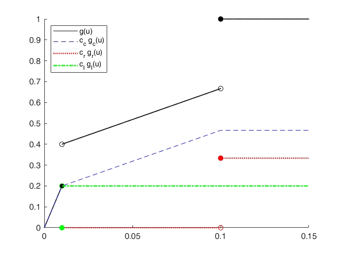
Figure 1: The decomposition of the distortion function $g(u)$ in right- and left-continuous parts scaled with $c_{r}$, $c_{l}$.

4.2 Results

The results of the numerical experiments are displayed in Tables 2 – 4. Throughout the experiment, we use $N=20000$ samples to determine the size and power of the tests. The parameter $n$ signifies the length of the considered time series, the parameter $m$ determines the number of considered cells. The level $\kappa$ in the construction of the approximate tests is set to $5\%$. Table 2 shows the results for AV@R, Table 2 compares these to Kratz et al. (2018). Table 4 shows the result of the backtest for GlueV@R and Table 4 for the distortion function that is neither right- nor left-continuous. We also provide a comparison of AV@R with the risk measure range value at risk (RV@R) in Appendix A.9.

Pearson
$L_{t}$	$n|m$	1	2	4	8	16	32	64
$\mathcal{N}$	250	0.97	1.26	1.39	1.67	2.26	3.01	4.35
	500	0.84	1.11	1.17	1.40	1.82	2.42	3.28
	1000	0.93	0.97	1.03	1.29	1.48	1.87	2.55
	2000	0.92	1.02	1.06	1.13	1.22	1.58	1.95
T3	250	16.31	24.17	28.97	27.41	38.34	38.00	36.83
	500	27.97	38.09	44.51	47.01	52.54	49.53	48.89
	1000	52.75	66.15	74.09	77.18	78.97	76.79	74.30
	2000	83.33	93.66	97.01	97.87	97.63	96.74	95.75
T5	250	17.72	23.61	26.16	26.12	29.53	36.35	37.66
	500	25.56	32.20	36.42	40.58	43.95	43.84	47.80
	1000	42.80	51.59	57.49	61.40	64.09	64.29	64.52
	2000	68.10	78.47	85.17	87.93	88.62	88.83	87.27
ST	250	35.58	44.04	49.95	49.21	52.42	60.90	58.81
	500	54.65	64.81	71.29	75.52	78.99	77.45	78.26
	1000	82.30	89.97	93.13	95.13	95.89	95.43	95.61
	2000	97.87	99.49	99.77	99.90	99.95	99.90	99.88

Nass
$L_{t}$	$n|m$	1	2	4	8	16	32	64
$\mathcal{N}$	250	0.79	0.95	1.05	1.12	1.01	1.08	1.05
	500	0.77	0.97	0.94	1.03	1.08	1.03	1.10
	1000	0.88	1.11	0.93	1.03	1.08	1.12	1.10
	2000	0.83	0.97	0.99	1.02	1.01	1.08	1.11
T3	250	16.26	21.61	21.97	25.54	20.41	20.89	22.73
	500	27.82	37.00	41.95	44.80	41.51	45.66	38.55
	1000	51.06	65.32	73.06	75.30	74.13	74.07	67.04
	2000	83.04	93.36	96.78	97.64	97.27	95.98	94.62
T5	250	17.31	20.83	20.21	22.53	19.60	20.44	19.46
	500	25.00	30.43	34.07	37.00	34.69	34.52	30.85
	1000	41.93	50.69	56.35	58.89	59.13	58.52	53.65
	2000	67.67	77.70	84.69	87.26	87.48	86.43	83.57
ST	250	35.43	41.40	41.73	46.53	42.03	43.10	43.64
	500	54.33	63.24	69.56	73.59	71.25	73.45	67.83
	1000	81.55	89.66	92.81	94.49	94.74	94.41	93.00
	2000	97.84	99.45	99.76	99.88	99.94	99.87	99.82

LRT
$L_{t}$	$n|m$	1	2	4	8	16	32	64
$\mathcal{N}$	250	1.36	0.94	0.79	0.42	0.09	0.01	0
	500	1.65	1.42	1.39	1.24	0.53	0.07	0
	1000	1.08	1.23	1.36	1.60	1.68	0.76	0.04
	2000	0.97	1.08	1.20	1.30	1.79	2.47	1.34
T3	250	22.83	22.89	22.32	14.74	6.35	0.52	0.01
	500	31.26	39.86	48.78	48.14	34.79	9.32	0.43
	1000	53.79	65.89	75.52	79.68	81.43	67.68	21.52
	2000	83.76	94.01	97.08	97.95	98.29	98.37	95.09
T5	250	15.85	16.90	16.65	11.09	5.07	0.56	0
	500	21.04	25.70	29.79	31.01	23.49	6.82	0.27
	1000	37.55	43.61	49.17	52.78	55.75	45.74	12.20
	2000	63.24	73.31	79.98	81.65	82.34	84.45	77.24
ST	250	30.84	35.43	37.67	30.90	19.61	03.91	0.07
	500	48.46	57.35	64.61	67.94	61.45	32.82	4.62
	1000	78.40	86.22	90.19	92.63	93.52	90.09	62.56
	2000	97.11	99.18	99.66	99.82	99.86	99.88	99.63

Table 1: Backtesting AV@R: Estimated size (for the hypothesis $H_{0}$ with distribution $\mathcal{N}$) and power in $\%$ (for the alternatives $H_{1}$ with distributions T3, T5, ST, respectively) for the Pearson test, Nass test and LRT. The size is represented as the fraction of the true size according to our simulation divided by the desired level $\kappa=5\%$. The colouring scheme for the size is as follows: Values between 0.8 - 1.2 are green, values between 0.9 - 1.1 are dark green; values above 1.5 are red, above 2 dark red. The colouring scheme for the power is adopted from Kratz et al. (2018): Green refers to a power $\geq 70\%$; light red indicates a power $\leq 30\%$; dark red indicates poor results with a power $\leq 10\%$.

Pearson
$L_{t}$	$n|m$	1	2	4	8	16	32	64
$\mathcal{N}$	250	0.78	0.94	1.12	1.70	2.10	2.82	4.30
	500	0.78	0.88	1.04	1.32	1.72	2.46	3.24
	1000	1.00	1.04	1.00	1.12	1.44	1.80	2.40
	2000	1.00	0.90	0.96	1.00	1.26	1.44	1.76
T3	250	12.21	13.97	18.77	6.61	5.94	11	2.63
	500	22.77	22.39	28.81	18.61	20.34	13.33	9.09
	1000	45.85	39.45	47.39	28.98	25.97	21.99	18.5
	2000	76.03	46.46	49.81	18.57	15.13	13.94	13.75
T5	250	13.62	13.41	15.96	5.32	7.13	9.35	3.46
	500	20.36	16.5	20.72	12.18	11.75	7.64	8
	1000	35.9	24.89	30.79	13.2	11.09	9.49	8.72
	2000	60.8	31.27	37.97	8.63	6.12	6.03	5.27
ST	250	30.18	25.14	31.05	10.51	13.72	14.6	8.31
	500	47.75	29.91	36.39	10.92	14.39	7.95	8.06
	1000	72.8	27.67	30.83	3.83	4.59	3.33	3.61
	2000	85.67	8.79	9.07	0.2	0.15	0.1	0.18

Nass
$L_{t}$	$n|m$	1	2	4	8	16	32	64
$\mathcal{N}$	250	0.78	0.70	1.00	0.94	1.02	1.00	0.96
	500	0.78	0.78	0.94	0.94	1.10	1.10	1.06
	1000	1.00	0.96	0.94	0.98	1.02	1.06	1.02
	2000	1.00	0.86	0.90	0.90	1.06	1.02	0.98
T3	250	12.66	16.01	9.87	10.74	7.01	7.69	9.13
	500	23.02	21.5	19.55	16.1	9.21	16.26	12.15
	1000	41.16	30.12	18.96	15	12.73	19.37	12.34
	2000	66.44	20.66	6.28	3.44	2.97	6.38	5.02
T5	250	13.21	13.13	7.41	8.43	6.2	6.04	6.46
	500	19.8	16.13	13.57	12.5	8.09	8.52	8.15
	1000	35.03	25.19	16.85	12.69	10.53	10.82	9.85
	2000	60.37	30.7	15.09	9.06	6.68	6.23	6.57
ST	250	30.03	26.1	15.43	16.03	11.83	12.4	12.94
	500	47.43	30.04	21.96	17.39	9.85	16.65	11.03
	1000	72.05	28.26	10.51	6.39	4.74	6.51	5.1
	2000	85.64	8.75	1.16	0.18	0.24	0.37	0.32

LRT
$L_{t}$	$n|m$	1	2	4	8	16	32	64
$\mathcal{N}$	250	1.50	2.00	1.34	0.46	0.14	0.02	0
	500	1.18	1.16	1.34	1.38	0.64	0.06	0
	1000	0.82	1.10	1.08	1.60	1.80	0.88	0.04
	2000	0.84	0.98	1.04	1.20	1.78	2.60	1.40
T3	250	12.53	-1.51	2.82	2.14	1.85	0.12	0.01
	500	21.76	13.66	9.88	5.74	5.69	1.52	0.13
	1000	44.09	18.69	11.22	5.58	4.23	5.18	6.52
	2000	67.26	14.51	3.88	1.85	1.29	0.87	1.69
T5	250	8.95	2.5	3.65	1.09	1.27	0.16	0
	500	14.54	10.2	6.19	4.81	3.59	1.42	0.07
	1000	32.35	17.51	11.27	6.88	5.35	3.84	2.7
	2000	57.44	25.31	12.28	6.85	3.94	2.45	2.64
ST	250	22.84	10.83	10.47	5.2	5.11	1.21	0.07
	500	40.56	21.45	11.71	8.94	7.55	5.62	1.42
	1000	71.5	23.92	8.69	4.63	2.42	2.59	8.46
	2000	87.31	7.58	1.16	0.32	0.26	0.08	0.03

Table 2: Backtesting AV@R: Comparison of the results in Table 2 to the results of Kratz et al. (2018). We display size and differences in power. The size is represented as the fraction of the true size according to Kratz et al. (2018) divided by the desired level $\kappa=5\%$. The colouring scheme for the size is as follows: Values between 0.8 - 1.2 are green, values between 0.9 - 1.1 are dark green; values above 1.5 are red, above 2 dark red. For the alternative T3, T5, and ST, the table shows the difference of the power of our method and the method of Kratz et al. (2018). The colouring scheme for the power is as follows: Dark green are notable improvements of the power $\geq 20\%$; light green are improvements $\geq 10\%$.

Pearson
$L_{t}$	$n|m$	1	2	4	8	16	32	64
$\mathcal{N}$	250	0.88	1.05	1.18	1.44	1.78	2.46	3.24
	500	0.87	1.04	1.06	1.20	1.46	1.87	2.38
	1000	0.93	0.96	1.03	1.15	1.26	1.44	1.94
	2000	0.98	0.97	1.00	1.03	1.17	1.28	1.51
T3	250	29.3	26.04	19.25	18.96	23.03	19.91	18.44
	500	60.01	60.38	49.2	43.65	40.1	35.18	31.48
	1000	93.08	94.11	90.53	87.19	79.04	69.84	60.94
	2000	99.93	99.97	99.89	99.87	99.67	98.15	94.65
T5	250	16.7	18.4	15.65	16.89	19.75	19.51	21.94
	500	29.37	30.71	26.66	29.03	29.07	28.42	28.76
	1000	52.85	56.72	52.3	53.93	52.75	50.77	46.67
	2000	83.76	87.16	84.84	87.35	86.29	83.06	78
ST	250	39.9	41.34	35.68	37.65	43.33	39.7	39.29
	500	68.42	71.82	66.81	67.35	67.27	65.3	62.91
	1000	94.6	96.18	95.25	95.33	94.45	92.6	90
	2000	99.92	99.97	99.98	100	99.97	99.93	99.73

Nass
$L_{t}$	$n|m$	1	2	4	8	16	32	64
$\mathcal{N}$	250	0.81	0.93	0.97	1.09	1.12	1.12	1.08
	500	0.85	0.97	0.95	1.00	1.07	1.10	1.06
	1000	0.91	0.93	0.97	1.04	1.02	1.05	1.15
	2000	0.97	0.93	0.96	0.96	1.04	1.08	1.04
T3	250	27.12	23.78	16.51	16.89	14.36	17.77	13.68
	500	60.01	59.04	47.24	40.16	35.45	32.56	25.81
	1000	93.08	93.91	89.94	85.86	76.88	66.17	57.1
	2000	99.93	99.97	99.89	99.86	99.6	97.84	93.49
T5	250	16.23	17.46	13.96	14.84	13.26	13.96	10.8
	500	29.37	29.97	25.48	26.71	25	23.76	19.86
	1000	52.84	56.19	51.25	52.25	50.18	46.19	40.33
	2000	83.56	87.03	84.49	86.9	85.42	81.41	74.99
ST	250	50.38	44.84	35.28	35.65	32.98	36.06	30.22
	500	75.36	76.41	68.63	66.25	63.83	62.02	55.15
	1000	97	97.42	96.04	95.42	93.96	91.27	88.14
	2000	99.96	100	99.98	100	99.97	99.92	99.68

LRT
$L_{t}$	$n|m$	1	2	4	8	16	32	64
$\mathcal{N}$	250	1.08	1.05	1.42	1.23	0.58	0.08	0
	500	1.13	1.17	1.26	1.60	1.72	0.80	0.05
	1000	1.01	1.03	1.14	1.30	1.81	2.46	1.40
	2000	1.01	1.02	1.06	1.10	1.38	2.14	3.90
T3	250	42.19	39.52	40	35.42	12.83	1.44	0.01
	500	67.25	69.66	66.42	69.22	66.22	34.17	2.08
	1000	94.55	95.83	94.49	94.24	93.8	93.45	71.55
	2000	99.93	99.97	99.93	99.97	99.91	99.83	99.86
T5	250	18.98	17.92	19.3	17.99	8.38	1.18	0.01
	500	27.46	29.94	29.22	33.61	33.92	18.53	1.32
	1000	51.34	55.83	53.42	54.66	57.35	60.63	40.72
	2000	83.32	86.92	85.3	87.03	85.81	85.69	88.4
ST	250	44.8	43.72	43.95	43.5	26.86	6.19	0.16
	500	68.62	73.04	71.3	75.11	75.69	57.18	12.13
	1000	94.7	96.5	95.91	96.43	96.53	96.99	90.08
	2000	99.92	99.97	99.98	100	99.96	99.97	99.97

Table 3: Backtesting GlueV@R: Estimated size (for the hypothesis $H_{0}$ with distribution $\mathcal{N}$) and power in $\%$ (for the alternatives $H_{1}$ with distributions T3, T5, ST, respectively) for the Pearson test, Nass test and LRT. The size is represented as the fraction of the true size according to our simulation divided by the desired level $\kappa=5\%$. The colouring scheme for the size is as follows: Values between 0.8 - 1.2 are green, values between 0.9 - 1.1 are dark green; values above 1.5 are red, above 2 dark red. The colouring scheme for the power is adopted from Kratz et al. (2018): Green refers to a power $\geq 70\%$; light red indicates a power $\leq 30\%$; dark red indicates poor results with a power $\leq 10\%$.

Pearson
$L_{t}$	$n|m$	1	2	4	8	16	32	64
$\mathcal{N}$	250	0.91	0.97	1.00	1.22	1.43	1.93	2.30
	500	1.02	0.92	1.07	1.11	1.23	1.44	1.88
	1000	1.06	1.02	1.06	1.06	1.09	1.30	1.52
	2000	0.96	1.02	0.94	1.03	1.09	1.06	1.22
T3	250	62.31	56,63	40.22	15.42	13.66	10.98	8.92
	500	94.67	93.06	87.89	68.13	47.84	30.08	19.8
	1000	99.94	99.95	99.89	99.41	97.72	85.58	58.99
	2000	100	100	100	100	100	100	99.27
T5	250	20.95	20.06	14.29	8.54	10.98	10.7	11.11
	500	41.06	40.21	33.11	20.04	21.55	19.13	16.5
	1000	72.12	73.24	67.47	52.55	51.34	42.45	35.06
	2000	96.58	97.15	96.4	91.7	91.38	85.29	74.42
ST	250	60.06	58.77	47.03	26.51	29.97	26.42	23.73
	500	92.67	92.54	88.77	74.05	67.87	56.88	47.83
	1000	99.86	99.94	99.82	99.4	98.7	95.3	87.76
	2000	100	100	100	100	100	100	99.96

Nass
$L_{t}$	$n|m$	1	2	4	8	16	32	64
$\mathcal{N}$	250	0.87	0.91	0.90	1.06	1.08	1.13	1.08
	500	0.97	0.88	1.01	1.00	1.00	1.05	1.11
	1000	1.04	0.99	1.02	0.99	0.98	1.09	1.09
	2000	0.95	1.00	0.92	1.00	1.04	0.97	1.00
T3	250	61.07	54.45	37.19	12.86	11.13	9.88	6.62
	500	93.72	92.41	87.04	65.86	43.77	26.51	17.62
	1000	99.94	99.95	99.88	99.36	97.37	83.04	54.73
	2000	100	100	100	100	100	100	99.14
T5	250	20.39	19.1	13.08	7.37	8.66	8.23	6.35
	500	39.68	39.11	31.98	18.67	19.61	16.18	12.67
	1000	72.03	72.81	67	51.48	49.75	39.6	31.21
	2000	96.54	97.11	96.33	91.47	90.94	84.33	72.28
ST	250	59.51	57.23	44.3	23.68	25.75	24.42	18.5
	500	91.72	92.01	88.11	72.21	64.9	53.16	43.88
	1000	99.86	99.93	99.82	99.36	98.58	94.48	85.74
	2000	100	100	100	100	100	100	99.96

LRT
$L_{t}$	$n|m$	1	2	4	8	16	32	64
$\mathcal{N}$	250	1.54	1.10	1.17	1.65	1.71	0.80	0.04
	500	1.07	1.05	1.17	1.38	1.83	2.49	1.37
	1000	1.12	1.07	1.09	1.10	1.32	2.16	3.79
	2000	0.98	1.02	0.97	1.05	1.15	1.36	2.69
T3	250	70.37	68.39	64.67	60.66	55.03	13.94	0.1
	500	95.55	95.47	93.66	88.75	88.31	86.59	41.03
	1000	99.98	99.97	99.95	99.79	99.64	99.34	99.26
	2000	100	100	100	100	100	100	100
T5	250	23.86	23.66	22.31	22.71	22.12	7.46	0.17
	500	42.74	43.38	40.33	34.53	39.87	42.01	17.36
	1000	74.04	75.52	71.97	63.42	64.29	65.74	71.6
	2000	96.97	97.4	97.04	94.11	94.09	91.54	91.32
ST	250	65.23	66.43	63.11	59.75	59.07	25.49	0.82
	500	93.35	94.42	92.84	88.36	89.5	89.27	60.48
	1000	99.89	99.95	99.89	99.81	99.69	99.43	99.56
	2000	100	100	100	100	100	100	100

Table 4: Backtesting the DRM corresponding to a distortion function that is neither left- nor right-continuous: Estimated size (for the hypothesis $H_{0}$ with distribution $\mathcal{N}$) and power in $\%$ (for the alternatives $H_{1}$ with distributions T3, T5, ST, respectively) for the Pearson test, Nass test and LRT. The size is represented as the fraction of the true size according to our simulation divided by the desired level $\kappa=5\%$. The colouring scheme for the size is as follows: Values between 0.8 - 1.2 are green, values between 0.9 - 1.1 are dark green; values above 1.5 are red, above 2 dark red. The colouring scheme for the power is adopted from Kratz et al. (2018): Green refers to a power $\geq 70\%$; light red indicates a power $\leq 30\%$; dark red indicates poor results with a power $\leq 10\%$.

Backtesting AV@R. Table 2 shows the size and power of the tests when backtesting AV@R. The size is represented as the fraction of the true size according to our simulation divided by the desired level $\kappa=5\%$. The size of the Pearson test is only close to the desired level for sufficiently small $m$. In the case of the LRT, the size of the test is not always very close to $\kappa$, sometimes smaller, sometimes larger. Table 2 shows the results of the approach of Kratz et al. (2018) for comparison. The qualitative behavior of the size of the Pearson and the LRT test is not very different for both methodologies. Both tests are not ideal for backtesting AV@R. In contrast, the size of Nass’ test is very close to desired level of $\kappa=5\%$ in all cases, as displayed in Table 2. This is qualitatively not very different from Kratz et al. (2018), see Table 2. This indicates that the Nass’ test is the preferred choice for backtesting AV@R, while the Pearson and the LRT test should not be chosen.

Table 2 also shows the power of our method for the different alternatives and various choices of the parameters $m$ and $n$. As expected, the power is good if $n$ is large. Most interesting is the Nass’ test. For $m$ smaller than $8$, the power exceeds for $n=500$ a value of $40\%$ for T3, $25\%$ for T5, and $66\%$ for ST, respectively. For $m$ smaller than $64$ and $n=2000$, the power exceeds $93\%$ for T3, $74\%$ for T5, and $99.6\%$ for ST, respectively.

In comparison to Kratz et al. (2018), our method improves the power of all tests for most case studies. Table 2 shows for the alternatives the difference between the power of our method and the results of Kratz et al. (2018). Positive numbers indicate that our approach improves the power. Except for one entry, all numbers are positive. In particular, for the Nass’ test our method uniformly improves the power substantially.

Comparing different risk measures. We now study the size across the three considered risk measures. The estimated size of the tests is shown for different $n$ and $m$ in Tables 2, 4 and 4. As before, the size is represented as the fraction of the true size according to our simulation divided by the desired level $\kappa=5\%$. The data clearly demonstrate that Nass’ test performs well in terms of approximating the desired level and clearly outperformes the Pearson and the LRT test in this respect. The latter two work well if $m$ is not too large and $n$ is not too small.

In all case studies, as expected, the power is best for $n$ large. Good backtests require $n$ to be larger than 500 to 1000 for the chosen hypothesis and alternatives. The best results are obtained for $2\leq m\leq 16$. There is no indication that Nass’ test performs worse than the other tests in correctly identifying the alternatives if they are true.

Conclusion. The Nass’ test outperforms the Pearson and the LRT test, since its size is generally close to the desired level and its overall power is not worse than or at least rather close to the power of the alternative tests across most case studies.

5 An Application to Asset-Liability Management

Financial institutions need to manage their risks arising from the evolution of their assets and liabilities. Asset-liability management (ALM) requires probabilistic models that enable a stochastic projection of the arising risks into the future. In this section, we apply our backtesting method to a company’s net asset value in order to validate risk measurements in an ALM model.

5.1 The Model

Inspired by Becker et al. (2014) and Hamm et al. (2020), we consider the assets and liabilities of a non-life insurance firm. Time is discrete and enumerated by $t=1,\dots,n$. Each time period could be interpreted as years, months, weeks or even days. Denote with $A_{t}$, $L_{t}$, $E_{t}$ the book value of assets, liabilities resp. the net asset value. At every point in time the value of the assets is equal to the liabilities and the net asset value, i.e. $A_{t}=L_{t}+E_{t}$.

Asset Model.

The market consists of two primary products, a riskless bond and a risky stock with price processes $B=(B_{t})_{t}$ and $S=(S_{t})_{t}$, respectively. We assume that $B_{t}=\exp(rt)$ and

$$S_{t}=\exp\left(\left(\mu-\frac{\sigma^{2}}{2}\right)t+\sigma W_{t}\right),$$

where $W_{t}$ is a Wiener process. At each point in time $t$, $\eta_{t}^{B}$ and $\eta_{t}^{S}$ denote the number of shares held in the bond and the stock, respectively. The resulting value of the asset portfolio is

$$A_{t}=\tilde{S}_{t}+\tilde{B}_{t}\quad\mbox{with }\;\tilde{S}_{t}=\eta_{t}^{S}S_{t},\;\tilde{B}_{t}=\eta_{t}^{B}B_{t}.$$

For simplicity, we assume that $r=0$.

Investment Strategy.

We assume that at the beginning of each period a fraction $b\in[0,1]$ of the book value of the liabilities and equity is invested into the stock, while the remaining fraction $1-b$ is invested into the bond. This implies that

$$\eta_{t}^{S}=b\cdot\frac{A_{t}}{S_{t}},\hskip 28.45274pt\eta_{t}^{B}=(1-b)\cdot A_{t}$$

Liability Model.

The insurer has a constant claims reserve $v$, such that $L_{t}=v$ at every point in time $t$. At the beginning of every time period the insurer takes in constant premiums $\pi$. Insurance claims at the end of every period $t$ are assumed to follow a collective model

$$C_{t}=\sum_{k=1}^{N_{t}}\xi_{t,k},\quad t=1,\dots,n,$$

where the frequencies $N_{t}\in\mathbb{N}$ and the severities $\xi_{t,k}\geq 0$, $k\in\mathbb{N}$, $t=1,\dots,n$ are independent.

Evolution of the Net Asset Value.

At time $t=1,\dots,n$ the insurer must pay $C_{t}$ for the claims incurred in the previous period and receives premium payments $\pi$ for the next period, i.e., the amount to be reinvested into the assets equals

$$A_{t}=\eta_{t-1}^{S}S_{t}+\eta_{t-1}^{B}B_{t}-C_{t}+\pi=A_{t-1}\cdot\left(b\cdot\frac{S_{t}}{S_{t-1}}+(1-b)\right)-C_{t}+\pi.$$

This can be rewritten in terms of the net asset value:

$$E_{t}=E_{t-1}+(E_{t-1}+v)\cdot b\cdot\left(\frac{S_{t}}{S_{t-1}}-1\right)-C_{t}+\pi.$$

5.2 Simulation Design

To illustrate our backtesting methodology in the context of the model, we consider as in Section 4.1.2 the GlueV@R risk measure. We choose the parameters $h_{1}=2/5$, $h_{2}=2/3$, $\alpha=0.05$ and $\beta=0.01$. Further case studies for $AV@R$ show similar results and are presented in Appendix A.11. Individual time periods are interpreted as days. The parameters defining the evolution of the assets are set to $\mu=\log(1.1)/360$, $\sigma=0.2/\sqrt{360}$ and $b=0.05$. In order to specify the liability model, we assume that $N_{t}$ are iid Poisson distributed random variables with parameter $\lambda>0$. Letting $\lambda=7$, expectation and variance are equal to $7$. The claims $\xi_{t,k}$ are iid exponentially distributed with parameter $1/\theta>0$. With $\theta=1000$, we obtain an expectation of $1000$ and a variance of $10^{6}$. We set $E_{0}=20000$. The premiums per day $\pi$ equal expected claims plus a $3\%$ safety margin, i.e., $\pi=1.03\lambda\theta$. The reserve is calculated as the expectation of the annual claims plus a $3\%$ margin, i.e., $v=360\cdot 1.03\lambda\theta$.

In this simple experimental ALM case study, we consider only the Nass test which showed the best performance in the case studies in Section 4 (just as in Kratz et al. (2018)) and constitutes the most promising methodology. The size of the Nass test is estimated as in Section 4. We consider the following alternatives labeled as NB, PAR and LOGN:

• We replace the Poisson distributed frequencies $N_{t}$ by frequencies $N^{\prime}_{t}$ with a negative binomial distribution with a number of failures $r\in\mathbb{N}$ and a success probability $q\in[0,1]$. Setting $q=1/(1+\lambda/r)$, $N^{\prime}_{t}$ and $N_{t}$ possess the same expectation. Letting $r=7$, the variance of the negative binomial distribution equals $\mathsf{Var}[N^{\prime}_{t}]=\lambda(1+\lambda/r)=14$.

• Claim sizes are given by $\xi^{1}_{t,k}-1$ with $\xi^{1}_{t,k}$ being Pareto distributed with scale $x_{0}=1$ and shape $a>0$. Setting $a=(\theta+1)/\theta$ guarantees that the expectation of the claim sizes $\xi^{1}_{t,k}-1$ of this alternative equals the expectation of the claim sizes $\xi_{t,k}$ of the null hypothesis.

• Under this alternative the claim sizes $\xi^{2}_{t,k}$ are log normally distributed with parameters $\mu\in\mathbb{R}$ and $\sigma>0$. We set $\mu=\log(\theta)-\sigma^{2}/2$ such that $\xi^{2}_{t,k}$ has the same expectation as $\xi_{t,k}$, and we choose $\sigma=1$ such that $\mathsf{Var}[\xi^{2}_{t,k}]=(\exp(\sigma^{2})-1)\theta^{2}\approx 1.7183\cdot 10^{6}$.

Nass
	$n|m$	1	2	4	8	16	32	64
Size	250	1.53	1.34	1.35	1.07	1.03	1.24	1.06
	500	1.57	1.36	1.19	1.21	1.19	1.14	1.19
	1000	1.77	1.46	1.30	1.22	1.18	1.16	1.25
	2000	1.76	1.50	1.34	1.25	1.27	1.20	1.25
NB	250	69.59	65.27	64.09	61.46	59.20	59.08	60.20
	500	89.44	89.56	84.74	84.72	82.61	79.70	82.08
	1000	99.02	98.88	98.45	98.28	96.74	96.49	95.97
	2000	99.99	100.00	99.99	100	99.98	99.93	99.90
PAR	250	97.60	98.31	98.27	97.97	97.75	97.72	97.29
	500	99.96	100	99.93	99.97	99.96	99.97	99.95
	1000	100	100	100	100	100	100	100
	2000	100	100	100	100	100	100	100
LOGN	250	53.11	51.63	50.85	47.94	47.83	46.28	44.05
	500	75.63	72.63	70.84	70.22	69.41	69.09	67.51
	1000	93.46	94.03	92.31	92.33	91.68	90.70	89.85
	2000	99.67	99.68	99.53	99.60	99.62	99.41	99.22

Table 5: Backtesting the ALM model: Estimated size and power in % for the alternatives NB, PAR and LOGN of the Nass test. The size is represented as the fraction of estimated size divided by the desired level $\kappa=5\%$. Values of the size between $0.9-1.1$ are dark green, between $0.8-1.2$ are light green, above $1.5$ are red and above $2$ dark red. For the power green refers to a power $\geq 70\%$; light red to a power $\leq 30\%$ and dark red indicates a power $\leq 10\%$.

5.3 Size and Power

We backtest the quantitative risk measurement of the net asset value process $(E_{t})_{t=1,\dots,n}$, applying GlueV@R. The numerical results are summarized in Table 5. We used $N=20000$ samples to estimate the size and the power of the Nass tests. The parameters $n$ and $m$ determine the number of observed data and the number of cells considered. As before, the desired level of the approximate test is set to $\kappa=5\%$.

Overall the size of the Nass test in the ALM model is slightly too large as displayed in the first panel of Table 5 where the quotient of the estimated size and the desired level $\kappa$ is shown. We see that the size is close to the desired level $\kappa$ for large $m$.

The overall power of the test is quite good. This is due to the fact that the null hypothesis and the considered alternatives are sufficiently different in all cases. The power is slightly higher for lower cell counts $m$ and also grows in the number of observed data $n$. For $n=500$, the power exceeds $89\%$ for NB, $99\%$ for PAR and $75\%$ for LOGN. The biggest power is estimated at $n=2000$ exceeding $99\%$ for all alternatives.

6 Conclusion

This paper proposes a multinomial backtesting methodology for distortion risk measures that is based on a stratification and randomization of risk levels, extending the non-randomized AV@R-backtest of Kratz et al. (2018). The method is applicable to a wide range of risk measures – being at the same time highly tractable. The best results are obtained for the Nass test. Numerical experiments based on artificial data demonstrate the good performance of the method if the null hypothesis and the considered alternatives are sufficiently different from each other. For AV@R, our randomized backtesting method improves upon the multinomial backtest of Kratz et al. (2018).

Future research should study the performance of DRM backtesting methods on the basis of real statistical data. Another interesting, but challenging question would be to compute lower bounds for the power of the method in terms of the number of data points and a measure of the distance between the null hypothesis and the alternative.

Appendix A Online Appendix

A.1 Comonotonic Risk Measures and DRMs

Definition A.1.

• A non decreasing function $g:[0,1]\rightarrow[0,1]$, with $g(0)=0$ and $g(1)=1$, is called a distortion function.

• Let $\mathsf{P}$ be a probability measure on $(\Omega,\mathcal{F})$ and $g$ be a distortion function. The monetary risk measure $\rho_{g}:\mathcal{X}\rightarrow\mathbb{R}$ defined as

  $$\rho_{g}(X):=\int_{-\infty}^{0}\left[g(\mathsf{P}(\{X>x\}))-1\right]dx+\int_{0}^{\infty}g(\mathsf{P}(\{X>x\}))dx,$$

  is called a DRM with respect to $g$.

DRMs can be expressed as mixtures of the quantile functions, if the distortion function is either left- or right-continuous. This is described in Dhaene et al. (2012).

Theorem A.2.

(i) If the distortion function $g$ is right-continuous, the DRM $\rho_{g}(X)$ is represented by a Lebesgue-Stieltje integral:

$$\rho_{g}(X)=\int_{[0,1]}q_{X}^{+}(1-u)\ dg(u)$$

where $q_{X}^{+}(u):=\sup\{x|F_{X}(x)\leq u\}$.
(ii) If the distortion function $g$ is left-continuous, the DRM $\rho_{g}(X)$ can be written as:

$$\rho_{g}(X)=\int_{[0,1]}q_{X}(1-u)\ dg(u)=\int_{[0,1]}q_{X}(u)\ d\bar{g}(u)$$

where $q_{X}(u)=\inf\{x|F_{X}(x)\geq u\}$ and $\bar{g}(q)=1-g(1-q)$, $0\leq q\leq 1$.

Several well known risk measures can be expressed as DRMs, see for example Cherny and Madan (2009), Balbás et al. (2009), Föllmer and Schied (2016), and Weber (2018). We consider some important examples in our applications.

Example A.3.

• Choosing the distortion function $g(u)=\mathds{1}_{\{\alpha<u\leq 1\}}$ yields the Value at Risk at level $\alpha\in(0,1)$:

  $$\rho_{g}(X)=V@R_{\alpha}(X):=\inf\{x|F_{X}(x)\geq 1-\alpha\}.$$

• The Average Value at Risk at level $\alpha$ corresponds to a DRM with distortion function $g(u)=\frac{u}{\alpha}\mathds{1}_{\{0\leq u\leq\alpha\}}+\mathds{1}_{\{u>\alpha\}}$:

  $$\rho_{g}(X)=AV@R_{\alpha}(X)=\frac{1}{\alpha}\int_{0}^{\alpha}V@R_{\lambda}(X)d\lambda.$$

• The GlueV@R is a DRM with distortion function

  $$g(u)=\begin{cases}\frac{h_{1}}{\beta}u\hskip 85.35826pt&\text{ if }0\leq u\leq\beta\\ h_{1}+\frac{h_{2}-h_{1}}{\alpha-\beta}(u-\beta)&\text{ if }\beta<u\leq\alpha\\ 1&\text{ if }\alpha<u\leq 1\end{cases},$$

  where $0\leq\beta<\alpha\leq 1$ are levels and $0\leq h_{1}\leq h_{2}\leq 1$ describe the corresponding distorted probabilities. The distortion function of the GlueV@R is a piecewise combination of the distortion functions of $V@R$ and $AV@R$. The GlueV@R can be expressed as a linear combination of these risk measures, i.e.,

  $$GlueV@R_{\beta,\alpha}^{h_{1},h_{2}}(X)=\rho_{g}(X)=w_{1}AV@R_{\beta}(X)+w_{2}AV@R_{\alpha}(X)+w_{3}V@R_{\alpha}(X),$$

  with $w_{1}=h_{1}-\frac{(h_{2}-h_{1})\beta}{\alpha-\beta}$, $w_{2}=\frac{h_{2}-h_{1}}{\alpha-\beta}\alpha$ and $w_{3}=1-w_{1}-w_{2}=1-h_{2}$.

Dhaene et al. (2012) show that every distortion function can be written as convex combination of a left- and right-continuous function. This is an important observation: If a distortion function $g$ is a convex combination of distortion functions $g_{1}$ and $g_{2}$, the distortion risk $\rho_{g}$ is a convex combination of the distortion risk measures $\rho_{g_{1}}$ and $\rho_{g_{2}}$, i.e., if $c_{1},c_{2}\geq 0$, $c_{1}+c_{2}=1$, then $g=c_{1}g_{1}+c_{2}g_{2}$ implies that $\rho_{g}=c_{1}\rho_{g_{1}}+c_{2}\rho_{g_{2}}.$

Theorem A.4.

Let $g$ be a distortion function. Then there exist right- and left-continuous distortion functions $h_{r}$, $h_{l}$ such that $g(u)=d_{r}h_{r}(u)+d_{l}h_{l}(u)\;\forall u\in[0,1]$ with $d_{r}$, $d_{l}\in[0,1]$, $d_{r}+d_{l}=1$.

The decomposition of the distortion function is not unique unless $g$ is a step function. A unique decomposition is provided in Theorem 2.2.

The link between comonotonic risk measures, the Choquet integral and DRMs is discussed in detail in Chapter 4 of Föllmer and Schied (2016) and Song and Yan (2009b). Comonotonic risk measures with an absolutely continuous capacity with respect to the underlying probability measure take the form of a DRM.

Name	Distortion	Closed form	Reference
$\mathrm{MINV@R}$	$1-(1-u)^{n}$	$-\mathsf{E}[\min\{-X_{1},\dots,-X_{n}\}]$	Cherny and Madan (2009)
		$=\mathsf{E}[\max\{X_{1},\dots,X_{n}\}]$	Föllmer and Schied (2016)
			Bannör and Scherer (2014)
$\mathrm{MAXV@R}$	$u^{1/n}$	$-\mathsf{E}[Y_{1}]$	Cherny and Madan (2009)
		such that	Föllmer and Schied (2016)
		$\max\{Y_{1},\dots,Y_{n}\}\sim-X$	Bannör and Scherer (2014)
$\mathrm{MINMAXV@R}$	$1-(1-u^{1/n})^{n}$	$-\mathsf{E}[\min\{Y_{1},\dots,Y_{n}\}]$	Cherny and Madan (2009)
		such that	Föllmer and Schied (2016)
		$\max\{Y_{1},\dots,Y_{n}\}\sim-X$	Bannör and Scherer (2014)
$\mathrm{MAXMINV@R}$	$(1-(1-u)^{n})^{1/n}$	$-\mathsf{E}[Y_{1}]$	Cherny and Madan (2009)
		such that	Föllmer and Schied (2016)
		$\max\{Y_{1},\dots,Y_{n}\}$	Bannör and Scherer (2014)
		$\sim\min\{-X_{1},\dots,-X_{n}\}$
$RV@R$	$\frac{u-\beta}{\alpha-\beta}\mathds{1}_{\{\beta<u\leq\alpha\}}+\mathds{1}_{\{u>\alpha\}}$	$\frac{1}{\alpha-\beta}\int_{\beta}^{\alpha}V@R_{\lambda}(X)d\lambda$	Bignozzi and Tsanakas (2016)
(Range $V@R$)	$0<\beta<\alpha<1$		Weber (2018), Li et al. (2018)
Proportional	$u^{1/\gamma}$	$\int_{0}^{\infty}(1-F_{X}(x))^{1/\gamma}dx,$	Wang (1995, 1996)
hazard transform	$\gamma>1$	if $X\geq 0$ a.s.	Guillen et al. (2018)
Dual power	$1-(1-u)^{\gamma}$	$\int_{0}^{\infty}1-F_{X}(x)^{\gamma}dx$,	Lynn Wirch and Hardy (1999)
transform	$\gamma>1$	if $X\geq 0$ a.s.	Guillen et al. (2018)
Gini’s principle	$(1-\theta)u+\theta u^{2}$	$\mathsf{E}[X]+\frac{\theta}{2}\mathsf{E}[|X-X_{1}|]$	Yitzhaki (1982),Wozabal (2014)
	$0<\theta<1$		Guillen et al. (2018)
Exponential	$\frac{1-\exp(-ru)}{1-\exp(-r)}$ if $r>0$	-	Methni and Stupfler (2017)
transform	$u$ if $r=0$		Dowd et al. (2008)
Inverse S-shaped	$a\left[\frac{u^{3}}{6}-\frac{\delta u^{2}}{2}+\left(\frac{\delta^{2}}{2}+\beta\right)u\right]$		Guegan and Hassani (2015)
polynomial	$a=\left(\frac{1}{6}-\frac{\delta}{2}+\frac{\delta^{2}}{2}+\beta\right)^{-1}$	-	Methni and Stupfler (2017)
of degree 3	$0<\delta<1,\beta\in\mathbb{R}$
Beta family	$\int_{0}^{u}\frac{t^{a-1}(1-t)^{b-1}}{B(a,b)}dt$	-	Samanthi and Sepanski (2019)
	$a,b>0$		Lynn Wirch and Hardy (1999)
Wang transform	$\Phi(\Phi^{-1}(u)-\Phi^{-1}(q))$	-	Wang (2000, 2001)
	$0<q<1$		Wozabal (2014)

Table 6: Further examples of distortion risk measures of a random variable $X$. Table 1 of the online appendix of Methni and Stupfler (2017) also provides these examples of distortion functions; we also include this table of examples as a convenient reference for the reader. In the third column, $X_{1},\dots,X_{n}$ denote independent copies of $X$, $n\in\mathbb{N}$; $Y_{1},\dots,Y_{n}$ are suitable i.i.d. random variables that satisfy the conditions that are specified in the third column of the table. $B$ denotes the beta function, $\Phi,\Phi^{-1}$ the distribution and quantile function of the standard normal distribution respectively.

A.2 Examples of DRMs

Examples of DRMs are provided in Table 6 which is taken from Methni and Stupfler (2017).

A.3 Proofs

A.3.1 Appendix to Section 2

Proof of Theorem 2.2.

As any distortion function $g$ is non decreasing, $g$ has at most countably many discontinuities. We define the sets of jumps by setting

$$R:=\{u\in[0,1]|g(u)-g(u-)>0\},\hskip 14.22636ptL:=\{u\in[0,1]|g(u+)-g(u)>0\}$$

with corresponding jump heights

$$g_{+}(u)=g(u)-g(u-),\hskip 28.45274ptg_{-}(u)=g(u+)-g(u),$$

respectively. Observe that $R$ and $L$ may possess a non empty intersection of points for which $g$ is neither right- nor left-continuous. We set

$$g_{sr}(u):=a\sum_{r\in R}g_{+}(r)\mathds{1}_{\{r\leq u\}},\hskip 28.45274ptg_{sl}(u):=b\sum_{l\in L}g_{-}(l)\mathds{1}_{\{l<u\}},$$

where $a,b$ are chosen such that $g_{sr},g_{sl}$ become distortion functions; for this purpose, we scale $g_{sr}$ and $g_{sl}$ such that $g_{sr}(1)=g_{sl}(1)=1$ by setting

$$a=\frac{1}{\sum_{r\in R}g_{+}(r)},\hskip 28.45274ptb=\frac{1}{\sum_{l\in L}g_{-}(l)}.$$

If $R=\emptyset$ and/or $L=\emptyset$ the original distortion function $g$ is right- or left-continuous, or continuous; in this case, we choose $a=0$ resp. $b=0$, and consider only the remaining parts. The functions $g_{sr}$ and $g_{sl}$ are right- resp. left-continuous step distortion functions. The continuous part of the decomposition is obtained by setting

$$g_{c}(u):=c\left(g(u)-\sum_{r\in R}g_{+}(r)\mathds{1}_{\{r\leq u\}}-\sum_{l\in L}g_{-}(l)\mathds{1}_{\{l<u\}}\right),\hskip 8.53581ptc:=\frac{1}{1-\sum_{r\in R}g_{+}(r)-\sum_{l\in L}g_{-}(l)}.$$

Finally, we obtain that

$$g(u)\;=\;\sum_{r\in R}g_{+}(r)\mathds{1}_{\{r\leq u\}}+\sum_{l\in L}g_{-}(l)\mathds{1}_{\{l<u\}}+\frac{1}{c}g_{c}(u)\;=\;\frac{1}{a}g_{sr}(u)+\frac{1}{b}g_{sl}(u)+\frac{1}{c}g_{c}(u),$$

where

$$\frac{1}{a}+\frac{1}{b}+\frac{1}{c}\;=\;1-\sum_{r\in R}g_{+}(r)-\sum_{l\in L}g_{-}(l)+\sum_{r\in R}g_{+}(r)+\sum_{l\in L}g_{-}(l)\;=\;1.$$

This decomposition is unique, since the functions $g_{rl}$ and $g_{sl}$ are unique for every distortion function. ∎

A.3.2 Appendix to Section 3.2

Proof of Lemma 3.1.

Since the conditional cumulative distribution functions $F_{M_{t}|M_{t-1},\dots,M_{1}}$ are continuous, we have for any $t$ that

$$\mathsf{P}(M_{t}>q_{M_{t}}^{t-1}(1-u)|M_{t-1},\dots,M_{1})=u.$$ (12)

Hence,

$$\mathsf{P}(L_{t}>q_{M_{t}}^{t-1}(1-u))\;\overset{L_{t}\overset{d}{=}M_{t}}{=}\;\mathsf{P}(M_{t}>q_{M_{t}}^{t-1}(1-u))\;=\;\mathsf{E}\left[{\mathsf{P}(M_{t}>q_{M_{t}}^{t-1}(1-u)|M_{t-1},\dots,M_{1})}\right]\;\overset{\eqref{eq:u=}}{=}\;u.$$

Thus, $\mathsf{E}[\mathds{1}_{t,j}|G_{t,j}]=G_{t,j}$ which implies $\mathsf{E}[\mathds{1}_{t,j}]\;=\;\mathsf{E}[G_{t,j}]\;=\;\frac{\mathsf{E}\left[G\mathds{1}_{\{G\in[\alpha_{j-1},\alpha_{j})\}}\right]}{g(\alpha_{j})-g(\alpha_{j-1})}.$ We define

$$\mathds{\tilde{1}}_{t,j}=\begin{cases}1\hskip 42.67912pt&\text{ if }M_{t}>q^{t-1}_{M_{t}}(1-G_{t,j})\\ 0&else.\end{cases},$$

and note that the processes $(\mathds{1}_{t,j})_{t}$ and $(\mathds{\tilde{1}}_{t,j})_{t}$ possess the same law, since, first, $M$ and $L$ do and, second, $(G_{t,j})_{t}$ is independent of $M$ and $L$. We set $\mathcal{G}_{t}=\sigma\{G_{s,j}:s\leq t,j=1,\dots,m+1\}$. We observe that

$$\mathsf{E}[\mathds{\tilde{1}}_{t,j}|M_{t-1},\dots,M_{1},\mathcal{G}_{t}]\;=\;\mathsf{E}[\mathds{\tilde{1}}_{t,j}|M_{t-1},\dots,M_{1},G_{t,j}]\;\overset{\eqref{eq:u=}}{=}\;G_{t,j},$$ (13)

where in the second step we use that $\mathds{\tilde{1}}_{t,j}$ is independent of $G_{t-1,j},\dots,G_{1,j}$ and $G_{t,k},\dots,G_{1,k}$ for $k\neq j$.

Next, for fixed $j=1,2,\dots,m+1$, we prove that the indicators $(\mathds{\tilde{1}}_{t,j})_{t}$ are independent. It suffices to show that for any $T\subseteq\{1,2,\dots,n\}$ we have that

$$\mathsf{E}\left[\prod_{t\in T}\mathds{1}_{t,j_{t}}\right]\;=\;\prod_{t\in T}\mathsf{E}[\mathds{1}_{t,j_{t}}]$$ (14)

with $j_{t}\in\{1,2,\dots,m+1\}$ for $t\in T$.

This can be shown by induction. Suppose that (14) holds for any $T$ such that $s\in T$ implies $s<t$. We set $j:=j_{t}$. Then

$$\mathsf{E}\left[\mathds{1}_{t,j}\prod_{s\in T}\mathds{1}_{s,j_{s}}\right] \;=\;\mathsf{E}\left[\mathds{\tilde{1}}_{t,j}\prod_{s\in T}\mathds{\tilde{1}}_{s,j_{s}}\right]\;=\;\mathsf{E}\left[\mathsf{E}\left[\mathds{\tilde{1}}_{t,j}\prod_{s\in T}\mathds{\tilde{1}}_{s,j_{s}}|M_{t-1},\dots,M_{1},\mathcal{G}_{t}\right]\right]$$

$$\;=\;\mathsf{E}\left[\prod_{s\in T}\mathds{\tilde{1}}_{s,j_{s}}\mathsf{E}\left[\mathds{\tilde{1}}_{t,j}|M_{t-1},\dots,M_{1},G_{t,j}\right]\right]\quad\hfill\mbox{\footnotesize(due to measurability and independence)}$$

$$\;\overset{\eqref{eq:compuxy}}{=}\;\mathsf{E}\left[\prod_{s\in T}\mathds{\tilde{1}}_{s,j_{s}}G_{t,j}\right]$$

$$\;=\;\mathsf{E}\left[\prod_{s\in T}\mathds{\tilde{1}}_{s,j_{s}}\right]\cdot\mathsf{E}\left[G_{t,j}\right]\quad\quad\quad\quad\quad\quad\quad\quad\mbox{\footnotesize(due to independence)}$$

$$\;=\;\mathsf{E}\left[\mathds{1}_{t,j}\right]\cdot\mathsf{E}\left[\prod_{s\in T}\mathds{1}_{s,j_{s}}\right]$$

∎

Proof of Lemma 3.2.

The random variable $X_{t}$ is a sum of the exception indicators $\mathds{1}_{t,j}$, $j=1,\dots,m+1$, for fixed $t=1,\dots,n$. Thus, the independence of $(X_{t})_{t=1,\dots,n}$ follows from the assumption of the independence of the vectors $(\mathds{1}_{t,j})_{j}$, $t=1,\dots,n$.

For $1\leq k\leq m$ we compute

$$\mathsf{P}(X_{t}=k) =\mathsf{P}\left(L_{t}>q^{t-1}_{M_{t}}(1-G_{m+2-k}),L_{t}\leq q^{t-1}_{M_{t}}(1-G_{m+1-k})\right)$$

$$=\mathsf{P}\left(q^{t-1}_{M_{t}}(1-G_{m+2-k})<L_{t}\leq q^{t-1}_{M_{t}}(1-G_{m+1-k})\right)$$

$$=\mathsf{P}\left(L_{t}\leq q^{t-1}_{M_{t}}(1-G_{m+1-k})\right)-\mathsf{P}\left(L_{t}\leq q^{t-1}_{M_{t}}(1-G_{m+2-k})\right)$$

$$=\frac{\mathsf{E}\left[G\mathds{1}_{\{G\in[\alpha_{m+1-k},\alpha_{m+2-k})\}}\right]}{g(\alpha_{m+2-k})-g(\alpha_{m+1-k})}-\frac{\mathsf{E}\left[G\mathds{1}_{\{G\in[\alpha_{m-k},\alpha_{m+1-k})\}}\right]}{g(\alpha_{m+1-k})-g(\alpha_{m-k})}.$$

For $k=0$ we have that

$$\mathsf{P}(X_{t}=0)=P(L_{t}\leq q^{t-1}_{M_{t}}(1-G_{m+1}))=1-\frac{\mathsf{E}\left[G\mathds{1}_{\{G\in[\alpha_{m},1)\}}\right]}{g(1)-g(\alpha_{m})}.$$

Therefore, $\mathsf{P}(X_{t}\leq k)=\sum_{i=0}^{k}\mathsf{P}(X_{t}=i)=1-\frac{\mathsf{E}\left[G\mathds{1}_{\{G\in[\alpha_{m-k},\alpha_{m-k+1})\}}\right]}{g(\alpha_{m-k+1})-g(\alpha_{m-k})}.$ ∎

Proof of Theorem 3.3.

Let $n_{0},n_{1},\dots,n_{m+1}\in\mathbb{N}$ such that $\sum n_{i}=n$. Then we have that

$$\mathsf{P}(O_{0}=n_{0},O_{1}=n_{1},\dots,O_{m+1}=n_{m+1})$$

$$=\mathsf{P}\left(\sum_{t=1}^{n}\mathds{1}_{\{X_{t}=0\}}=n_{0},\sum_{t=1}^{n}\mathds{1}_{\{X_{t}=1\}}=n_{1},\dots,\sum_{t=1}^{n}\mathds{1}_{\{X_{t}=m+1\}}=n_{m+1}\right)$$

$$=\sum_{\pi\in\Pi}\mathsf{P}\big{(}X_{\pi(0)}=0,\dots,X_{\pi(n_{0})}=0,X_{\pi(n_{0}+1)}=1,\dots,X_{\pi(n_{0}+n_{1})}=1,$$

$$\dots,X_{\pi(n_{0}+\dots+n_{m}+1)}=m+1,\dots X_{\pi(n_{0}+\dots+n_{m+1})}=m+1\big{)}$$

$$=\sum_{\pi\in\Pi}\prod_{k=0}^{m+1}p_{k}^{n_{k}}.$$

Here, $\Pi$ is the set of permutations of $\{1,\dots,n\}$ such that $n_{0}$ of the $X_{t}$ are equal to $0$, $n_{1}$ of the $X_{t}$ are equal to $1$ and so on. We have $n!$ possible permutations of the set $\{1,\dots,n\}$, where the $n_{0}!$ permutations of the set $\{t|X_{t}=0\}$ are indistinguishable. The same holds for $n_{1}$, $n_{2}$, etc. We conclude that

$$P(O_{0}=n_{0},O_{1}=n_{1},\dots,O_{m+1}=n_{m+1})=\frac{n!}{n_{0}!n_{1}!\dots n_{m+1}!}\prod_{k=0}^{m+1}p_{k}^{n_{k}},$$

which is the probability mass function of $MN(n,(p_{0},p_{1},p_{2},\dots,p_{m+1}))$ for the corresponding probabilities $p_{k}$. ∎

A.4 Statistical Tests

This section describes multinomial tests for the null hypotheses (6) and (9) which we review for the convenience of the reader. Cai and Krishnamoorthy (2006) provide a more detailed discussions, and the tests are also reviewed and used in Kratz et al. (2018).

We adopt three well-known approximate tests: Pearson’s $\chi^{2}$-test, Nass’ $\chi^{2}$-test, and the likelihood ratio test. We briefly review the design of these tests.

A.4.1 Pearson’s $\chi^{2}$-Test

A standard test for the hypothesis that $O=(O_{0},O_{1},\dots,O_{m+1})\sim\mathrm{MN}(n,(p_{0},p_{1},\dots,p_{m+1}))$ relies on results obtained by Pearson (1900). Since $\mathsf{E}[O_{k}]=np_{k}$, $k=0,\dots,m+1$, the observed frequencies of the cell counts should be close to $np_{k}$ for a sufficiently large $n$. The cumulated relative squared deviations of the observations from the mean

$$S_{m+1}:=\sum_{k=0}^{m+1}\frac{(O_{k}-np_{k})^{2}}{np_{k}},$$

are for large $n$ approximately $\chi^{2}_{m+1}$-distributed. Pearson’s $\chi^{2}$-test at level $\kappa\in(0,1)$ rejects the hypothesis if

$$S_{m+1}\;>\;F^{-1}_{\chi^{2}_{m+1}}(1-\kappa),$$

where $F^{-1}_{\chi^{2}_{m+1}}(1-\kappa)$ is the $\kappa$-quantile of the $\chi^{2}_{m+1}$ distribution. This test is the probably most widely used multinomial test that typically performs well if the cell probabilities are not too small.

A.4.2 Nass’ $\chi^{2}$-Test

Nass (1959) suggests a finite sample correction of Pearson’s $\chi^{2}$-test. Instead of approximating the distribution of $S_{m+1}$ with a $\chi^{2}_{m+1}$-distribution, Nass (1959) proposes to use a distribution that depends on $n$, namely the distribution of $\frac{1}{c}Z$ with $Z\sim\chi^{2}_{\nu}$ where

$$c\;= \;\frac{2\mathsf{E}[S_{m+1}]}{\mathrm{Var}(S_{m+1})},\quad\nu\;=\;cE[S_{m+1}],\quad E[S_{m+1}]\;=\;m+1,$$

$$\mathrm{Var}(S_{m+1})\;=\; \;2(m+1)\;-\;\frac{m^{2}+6m+6}{n}\;\;+\;\;\sum_{k=0}^{m+1}\frac{1}{n\cdot p_{k}}.$$

Since $c\rightarrow 1$ and $\nu\rightarrow m+1$ as $n\to\infty$, the distributions used in the finite sample approximation are asymptotically equal to the asymptotic distribution known from Pearson’s $\chi^{2}$-test. But in Nass’ $\chi^{2}$-test the distribution of the approximating $\frac{1}{c}Z$ matches for each $n$ the first two moments of the distribution of $S_{m+1}$, while $\chi^{2}_{m+1}$ matches only the first moment. One can conjecture that this might typically lead to a better approximation than Pearson’s test.

On the basis of this finite sample correction that matches the first two moments, the null hypothesis is rejected in Nass’ $\chi^{2}$-test at level $\kappa\in(0,1)$, if $cS_{m+1}>F^{-1}_{\chi^{2}_{\nu}}(1-\kappa).$

A.4.3 Likelihood Ratio Test

A likelihood ratio test (LRT) is a standard procedure in hypothesis testing that compares the ratio of the likelihood of the sample under the null hypothesis and without any restriction. More precisely, suppose that $\Theta$ is the parameter set and that $\Theta_{0}\subseteq\Theta$ denotes the null hypothesis. By $X$ we denote the observations and by $p_{\vartheta}$ the likelihood function for $\vartheta\in\Theta$. The corresponding likelihood ratio is given by

$$\lambda(X)=\frac{\sup_{\vartheta\in\Theta_{0}}p_{\vartheta}(X)}{\sup_{\vartheta\in\Theta}p_{\vartheta}(X)}.$$

The asymptotic distribution of $-2\log\lambda(X)$ for the number of samples going to $\infty$ can conveniently be characterized in models that satisfy suitable regularity conditions, see e.g. Section 10.3 of Casella and Berger (2002).

A result of this type holds in particular, if $\Theta$ includes all multinomial distributions for $n$ trials and $m+2$ possible outcomes and the null hypothesis contains only the single distribution $\mathrm{MN}(n,(p_{0},p_{1},\dots,p_{m+1}))$. In this case, the LRT statistic is

$$R\;=\;2\sum_{k=0}^{m+1}O_{k}\log\left(\frac{O_{k}}{np_{k}}\right)$$

with an asymptotic $\chi_{m+1}^{2}$-distribution for $n\to\infty$. The corresponding LRT with level $\kappa\in(0,1)$ rejects the null hypothesis if $R>F^{-1}_{\chi_{m+1}^{2}}(1-\kappa).$

A.5 The Skewed t-Distribution of Fernández and Steel (1998)

Consider the probability density function (pdf) $g_{\nu}$ of the t-distribution with $\nu$ degrees of freedom as

$$g_{\nu}(x)=\frac{\Gamma\left(\frac{\nu+1}{2}\right)}{\sqrt{\nu\pi}\Gamma\left(\frac{\nu}{2}\right)}\left(1+\frac{x^{2}}{\nu}\right)^{-\frac{\nu+1}{2}}.$$

Fernández and Steel (1998) proposes a class of skewed distributions with the pdf

$$f_{\nu,\gamma}(x)=\frac{2}{\gamma+\frac{1}{\gamma}}\left(g_{\nu}\left(\frac{x}{\gamma}\right)\mathds{1}_{\{x\in[0.\infty)\}}+g_{\nu}(\gamma x)\mathds{1}_{\{x\in(-\infty.0]\}}\right)$$

for $\gamma\in(0.\infty)$.
For the simulation we need to determine the expectation and variance of the skewed t-distribution defined above. From Fernández and Steel (1998) we know that if $X\sim f_{\nu,\gamma}(x)$ then

$$E[X^{r}]=M_{r}\frac{\gamma^{r+1}+\frac{(-1)^{r}}{\gamma^{r+1}}}{\gamma+\frac{1}{\gamma}}$$

where $M_{r}=\int_{0}^{\infty}s^{r}2g_{\nu}(s)ds.$ With $Y\sim g_{\nu}(s)$, we have that (see Robert (2014) for the expectation of $|Y|$)

$$M_{1}\;=\;\int_{0}^{\infty}2s\frac{\Gamma\left(\frac{\nu+1}{2}\right)}{\sqrt{\nu\pi}\Gamma\left(\frac{\nu}{2}\right)}\left(1+\frac{x^{2}}{\nu}\right)^{-\frac{\nu+1}{2}}ds\\ \;=\;2E[|Y|]\\ \;=\;\frac{2\nu}{(\nu-1)\sqrt{\nu\pi}}\frac{\Gamma\left(\frac{\nu+1}{2}\right)}{\Gamma\left(\frac{\nu}{2}\right)}.$$

As $g_{\nu}(s)$ is symmetric we have

$$M_{2} =\int_{0}^{\infty}2s^{2}g_{\nu}(s)ds=\int_{0}^{\infty}s^{2}g_{\nu}(s)ds+\int_{-\infty}^{0}s^{2}g_{\nu}(-s)ds$$

$$=\int_{-\infty}^{\infty}s^{2}g_{\nu}(s))ds=E[Y^{2}]=\frac{\nu}{\nu-2}.$$

Now we can calculate the first two non centered moments of $X\sim f_{\nu}(x)$ as

$$E[X] =\left(\gamma-\frac{1}{\gamma}\right)\frac{2\nu}{(\nu-1)\sqrt{\pi\nu}}\frac{\Gamma\left(\frac{\nu+1}{2}\right)}{\Gamma\left(\frac{\nu}{2}\right)},$$

$$E[X^{2}] =\frac{\nu}{\nu-2}\frac{\gamma^{3}+\frac{1}{\gamma^{3}}}{\gamma+\frac{1}{\gamma}},$$

where the second moment exists if $\nu>2$. So the variance of $X$ is given as

$$\mathrm{Var}(X) =E[X^{2}]-E[X]^{2}$$

$$=\frac{\nu}{\nu-2}\frac{\gamma^{3}+\frac{1}{\gamma^{3}}}{\gamma+\frac{1}{\gamma}}-\left(\left(\gamma-\frac{1}{\gamma}\right)\frac{2\nu}{(\nu-1)\sqrt{\pi\nu}}\frac{\Gamma\left(\frac{\nu+1}{2}\right)}{\Gamma\left(\frac{\nu}{2}\right)}\right)^{2}.$$

To sample from $f_{\nu,\gamma}(x)$, we propose an acceptance-rejection algorithm with sampling distribution $g_{\nu}(x)$. For this to work we need to calculate $k>0$ such that

$$k \geq\frac{f_{\nu,\gamma}(x)}{g_{\nu}(x)}=\frac{\gamma+\frac{1}{\gamma}}{2}\frac{\left(1+\frac{x^{2}}{\nu}\right)^{-\frac{\nu+1}{2}}}{\left(1+\frac{x^{2}}{\gamma^{2}\nu}\right)^{-\frac{\nu+1}{2}}\mathds{1}_{\{x\in[0.\infty)\}}+\left(1+\frac{x^{2}\gamma^{2}}{\nu}\right)^{-\frac{\nu+1}{2}}\mathds{1}_{\{x\in(-\infty.0)\}}}.$$

We distinguish the following two cases.

• $x\geq 0$: we require that

  $$k \geq\frac{\gamma+\frac{1}{\gamma}}{2}\left(\frac{1+\frac{x^{2}}{\nu}}{1+\frac{x^{2}}{\gamma^{2}\nu}}\right)^{-\frac{\nu+1}{2}}.$$

  The function $x^{-\frac{\nu+1}{2}}$ is strictly falling on $x\in(0.\infty)$ and the argument of the function above is positive. Thus, we find $k$ by minimizing the argument

  $$i(x):=\frac{1+\frac{x^{2}}{\nu}}{1+\frac{x^{2}}{\gamma\nu}}.$$

  If $\gamma>1$, $i(x)$ is strictly decreasing and the maximum is found at $\lim_{x\rightarrow 0+}i(x)$. On the other hand, if $\gamma\in(0.1)$ the function is strictly monotone increasing and the maximum is $\lim_{x\rightarrow\infty}i(x)$. We can calculate this limit as

  $$\lim_{x\rightarrow\infty}\frac{1+\frac{x^{2}}{\nu}}{1+\frac{x^{2}}{\gamma^{2}\nu}}=\lim_{x\rightarrow\infty}\underbrace{\frac{1}{1+\frac{x^{2}}{\gamma^{2}\nu}}}_{\rightarrow 1}+\underbrace{\frac{1}{\nu\left(\frac{1}{x^{2}}+\frac{1}{\gamma^{2}\nu}\right)}}_{\rightarrow\gamma^{2}}=1+\gamma^{2}.$$

  Consequently, for $x\geq 0$ we have that

  $$\frac{\gamma+\frac{1}{\gamma}}{2}\left(\frac{1+\frac{x^{2}}{\nu}}{1+\frac{x^{2}}{\gamma^{2}\nu}}\right)^{-\frac{\nu+1}{2}}\leq\begin{cases}\frac{\gamma+\frac{1}{\gamma}}{2}(1+\gamma^{2})^{-\frac{\nu+1}{2}}\hskip 14.22636pt&\gamma<1\\ 1&\gamma=1\\ \frac{\gamma+\frac{1}{\gamma}}{2}&\gamma>1.\end{cases}$$

• $x<0$: we want to determine $k$ such that

  $$k\geq\frac{\gamma+\frac{1}{\gamma}}{2}\left(\frac{1+\frac{x^{2}}{\nu}}{1+\frac{x^{2}\gamma^{2}}{\nu}}\right)^{-\frac{\nu+1}{2}}.$$

  Using the same reasoning as above we minimize the argument

  $$i(x):=\frac{1+\frac{x^{2}}{\nu}}{1+\frac{x^{2}\gamma^{2}}{\nu}}$$

  to find the maximum of the density quotient. If $\gamma<1$ we find the minimum of $i(x)$ at $\lim_{x\rightarrow 0-}i(x)$. We have that

  $$\lim_{x\rightarrow 0-}\frac{1+\frac{x^{2}}{\nu}}{1+\frac{x^{2}\gamma^{2}}{\nu}}=\lim_{x\rightarrow 0-}\frac{1}{1+\frac{x^{2}\gamma^{2}}{\nu}}+\frac{1}{\nu\left(\frac{1}{x^{2}}+\frac{\gamma^{2}}{\nu}\right)}=1+\frac{1}{\gamma^{2}}.$$

  Therefore,

  $$\frac{\gamma+\frac{1}{\gamma}}{2}\left(\frac{1+\frac{x^{2}}{\nu}}{1+\frac{x^{2}\gamma^{2}}{\nu}}\right)^{-\frac{\nu+1}{2}}\leq\begin{cases}\frac{\gamma+\frac{1}{\gamma}}{2}\left(\frac{1}{\gamma^{2}}\right)^{-\frac{\nu+1}{2}}\hskip 28.45274pt&\gamma>1\\ 1&\gamma=1\\ \frac{\gamma+\frac{1}{\gamma}}{2}&\gamma<1\end{cases}.$$

From this computation, we determine $k$ as follows: if $\gamma\geq 1$ we set

$$k:=\max\left\{\frac{\gamma+\frac{1}{\gamma}}{\frac{\gamma+\frac{1}{\gamma}}{2}}\left(\frac{1}{\gamma^{2}}\right)^{-\frac{\nu+1}{2}}\right\}=\frac{\gamma+\frac{1}{\gamma}}{2}\gamma^{\nu+1};$$

if $\gamma<1$ we set

$$k:=\max\left\{\frac{\gamma+\frac{1}{\gamma}}{2}\frac{\gamma+\frac{1}{\gamma}}{2}\left(1+\gamma^{2}\right)^{-\frac{\nu+1}{2}}\right\}=\frac{\gamma+\frac{1}{\gamma}}{2}.$$

A.6 Computations for Section 4.1.1

Consider the distortion function $g(u)=\frac{u}{\alpha}\mathds{1}_{\{0\leq u<\alpha\}}+\mathds{1}_{\{u\geq\alpha\}}$ of the AV@R at level $\alpha$. For $G\sim g$ and $0\leq a<b\leq 1$ we can calculate $\mathsf{E}[G\mathds{1}_{\{G\in[a,b)\}}]$ by considering the following cases:

• if $a,b<\alpha$,

  $$\mathsf{E}\left[G\mathds{1}_{\{G\in[a,b)\}}\right]=\int_{a}^{b}u\frac{1}{\alpha}du=\frac{1}{2\alpha}(b^{2}-a^{2});$$

• if $a<\alpha,b\geq\alpha$,

  $$\mathsf{E}\left[G\mathds{1}_{\{G\in[a,b)\}}\right]=\int_{a}^{\alpha}u\frac{1}{\alpha}du=\frac{1}{2\alpha}(\alpha^{2}-a^{2});$$

• if $a,b\geq\alpha$,

  $$\mathsf{E}\left[G\mathds{1}_{\{G\in[a,b)\}}\right]=0.$$

Let $\alpha_{0},\alpha_{1},\dots,\alpha_{m}$ be a partition of $[0,\alpha]$, where $\alpha_{m}\leq\alpha$ and set $\alpha_{m+1}=1$. Plugging this in the definition of the probabilities $p_{i}$ in Theorem 3.3, we obtain

$$p_{0} =1-\frac{\mathsf{E}[G\mathds{1}_{\{G\in[\alpha_{m},1)\}}]}{g(1)-g(\alpha_{m})}$$

$$=1-\frac{\frac{1}{2\alpha}(\alpha^{2}-\alpha_{m}^{2})}{1-\frac{\alpha_{m}}{\alpha}};$$

$$p_{k} =\frac{E\left[G\mathds{1}_{\{G\in[\alpha_{m+1-k},\alpha_{m+2-k})\}}\right]}{g(\alpha_{m+2-k})-g(\alpha_{m+1-k})}-\frac{E\left[G\mathds{1}_{\{G\in[\alpha_{m-k},\alpha_{m+1-k})\}}\right]}{g(\alpha_{m+1-k})-g(\alpha_{m-k})}$$

$$=\frac{\frac{1}{2\alpha}\left(\alpha_{m+2-k}^{2}-\alpha_{m+1-k}^{2}\right)}{\frac{1}{2\alpha}(\alpha_{m+2-k}-\alpha_{m+1-k})}-\frac{\frac{1}{2\alpha}\left(\alpha_{m+1-k}^{2}-\alpha_{m-k}^{2}\right)}{\frac{1}{2\alpha}(\alpha_{m+1-k}-\alpha_{m-k})}$$

$$=\frac{\left(\alpha_{m+2-k}^{2}-\alpha_{m+1-k}^{2}\right)}{(\alpha_{m+2-k}-\alpha_{m+1-k})}-\frac{\left(\alpha_{m+1-k}^{2}-\alpha_{m-k}^{2}\right)}{(\alpha_{m+1-k}-\alpha_{m-k})};\mbox{ and }$$

$$p_{m+1} =\frac{\mathsf{E}[G\mathds{1}_{\{G\in[0,\alpha_{1})\}}]}{g(\alpha_{1})}$$

$$=\frac{\frac{1}{2\alpha}\alpha_{1}^{2}}{\frac{\alpha_{1}}{\alpha}}=\frac{\alpha_{1}}{2},$$

where $k\in\{1,\dots,m\}$.

A.7 Computations for Section 4.1.2

Recall the GlueV@R risk measure introduced in Example A.3 corresponds to the distortion function

$$g(u)=\begin{cases}\frac{h_{1}}{\beta}u\hskip 85.35826pt&\text{ if }0\leq u\leq\beta\\ h_{1}+\frac{h_{2}-h_{1}}{\alpha-\beta}(u-\beta)&\text{ if }\beta<u\leq\alpha\\ 1&\text{ if }\alpha<u\leq 1\end{cases}.$$

where $0\leq\beta\leq\alpha\leq 1$ and $0\leq h_{1}\leq h_{2}\leq 1$. The partition is again set such that $(\alpha_{1},\dots,\alpha_{m})$ are equidistant in $[0,\alpha]$ and $\alpha_{0}=0$, $\alpha_{m+1}=1$.

To sample from $G|G\in[\alpha_{j},\alpha_{j+1})$ for $G\sim g$, we use the inverse transform method. If $U\sim\mathrm{unif}(0,1)$, then we have that $q_{g_{c}}(U)\sim g$. If we let $V$ be the restriction of $U$ to the interval $[\alpha_{j},\alpha_{j+1})$, as

$$V:=g(\alpha_{j})+(g(\alpha_{j+1})-g(\alpha_{j}))U,$$

we obtain that $q_{g_{c}}(V)$ is distributed as $G|G\in[\alpha_{j},\alpha_{j+1})$. The left quantile function $q_{g_{c}}$ of the distrotion function $g$ can be calculated as

$$q_{g_{c}}(v)=\begin{cases}\frac{\beta}{h_{1}}v\hskip 28.45274pt&,v\in[0,h_{1})\\ \beta+\frac{\alpha-\beta}{h_{2}-h_{1}}(v-h_{1})&,v\in[h_{1},h_{2}]\\ \alpha&,v\in(h_{2},1].\end{cases}$$

Now we can compute the probabilities $p_{k}$ from Theorem 3.3. The distortion function of the Glue-V@R defines the probability $\mathsf{P}$ with an atom at $\alpha$, where $\mathsf{P}(G=\alpha)=1-h_{2}$. For the absolutely continuous part of $P$ we have

$$dg(u)=\begin{cases}\frac{h_{1}}{\beta}du&\,u\in[0,\beta)\\ \frac{h_{2}-h_{1}}{\alpha-\beta}du&\,u\in[\beta,\alpha)\\ 0&\,u\in[\alpha,1].\end{cases}$$

The computation of the $p_{k}$ requires calculating $E\left[G\mathds{1}_{\{G\in[\alpha_{j},\alpha_{j+1})\}}\right]$ in the following five cases.

• $\alpha_{j}\in[0,\beta)$, $\alpha_{j+1}\in[0,\beta)$:

  $$\frac{\mathsf{E}\left[G\mathds{1}_{\{G\in[\alpha_{j},\alpha_{j+1})\}}\right]}{g(\alpha_{j+1})-g(\alpha_{j})} =\frac{\int_{\alpha_{j}}^{\alpha_{j+1}}u\frac{h_{1}}{\beta}du}{\frac{h_{1}}{\beta}(\alpha_{j+1}-\alpha_{j})}=\frac{1}{2}(\alpha_{j+1}-\alpha_{j}).$$

• $\alpha_{j}\in[0,\beta)$, $\alpha_{j+1}\in[\beta,\alpha)$:

  $$\frac{\mathsf{E}\left[G\mathds{1}_{\{G\in[\alpha_{j},\alpha_{j+1})\}}\right]}{g(\alpha_{j+1})-g(\alpha_{j})} =\frac{\int_{\alpha_{j}}^{\beta}udg(u)+\int_{\beta}^{\alpha_{j+1}}udg(u)}{h_{1}+\frac{h_{2}-h_{1}}{\alpha-\beta}(\alpha_{j+1}-\beta)-\frac{h_{1}}{\beta}\alpha_{j}}=\frac{\frac{h_{1}}{\beta}(\beta-\alpha_{j})^{2}+\frac{h_{2}-h_{1}}{2(\alpha-\beta)}(\alpha_{j+1}-\beta)^{2}}{h_{1}+\frac{h_{2}-h_{1}}{\alpha-\beta}(\alpha_{j+1}-\beta)-\frac{h_{1}}{\beta}\alpha_{j}}.$$

• $\alpha_{j}\in[0,\beta)$, $\alpha_{j+1}\in[\alpha,1)$:

  $$\frac{\mathsf{E}\left[G\mathds{1}_{\{G\in[\alpha_{j},\alpha_{j+1})\}}\right]}{g(\alpha_{j+1})-g(\alpha_{j})} =\frac{\frac{h_{1}}{\beta}\int_{\alpha_{j}}^{\beta}udu+\frac{h_{2}-h_{1}}{\alpha-\beta}\int_{\beta}^{\alpha}udu+\alpha\mathsf{P}(G=\alpha)}{1-\frac{h_{1}}{\beta}\alpha_{j}}$$

  $$=\frac{\frac{h_{1}}{2\beta}(\beta-\alpha_{j})^{2}+\frac{h_{2}-h_{1}}{2}(\alpha-\beta)+(1-h_{2})\alpha}{1-\frac{h_{1}}{\beta}\alpha_{j}}.$$

• $\alpha_{j}\in[\beta,\alpha)$, $\alpha_{j+1}\in[\beta,\alpha)$:

  $$\frac{\mathsf{E}\left[G\mathds{1}_{\{G\in[\alpha_{j},\alpha_{j+1})\}}\right]}{g(\alpha_{j+1})-g(\alpha_{j})} =\frac{\frac{h_{2}-h_{1}}{\alpha-\beta}\int_{\alpha_{j}}^{\alpha_{j+1}}udu}{h_{1}+\frac{h_{2}-h_{1}}{\alpha-\beta}(\alpha_{j+1}-\beta)-h_{1}-\frac{h_{2}-h_{1}}{\alpha-\beta}(\alpha_{j}-\beta)}=\frac{1}{2}(\alpha_{j+1}-\alpha_{j}).$$

• $\alpha_{j}\in[\beta,\alpha)$, $\alpha_{j+1}\in[\alpha,1)$:

  $$\frac{\mathsf{E}\left[G\mathds{1}_{\{G\in[\alpha_{j},\alpha_{j+1})\}}\right]}{g(\alpha_{j+1})-g(\alpha_{j})} =\frac{\frac{h_{2}-h_{1}}{\alpha-\beta}\int_{\beta}^{\alpha}udu+\alpha\mathsf{P}(G=\alpha)}{1-h_{1}+\frac{h_{2}-h_{1}}{\alpha-\beta}(\alpha_{j}-\beta)}=\frac{\frac{h_{2}-h_{1}}{2}(\alpha-\beta)+\alpha(1-h_{2})}{1-h_{1}+\frac{h_{2}-h_{1}}{\alpha-\beta}(\alpha_{j}-\beta)}.$$

We can plug these calculations in Theorem 3.3 to obtain $p_{k}$ for the multinomial distribution of the cell counts $O$.

A.8 Computations for Section 4.1.3

We consider the distortion function

$$g(u):=\begin{cases}\frac{h_{1}}{\beta}u\hskip 85.35826pt&u\in[0,\beta]\\ h_{2}+\frac{h_{3}-h_{2}}{\alpha-\beta}(u-\beta)&u\in(\beta,\alpha)\\ 1&u\in[\alpha,1]\end{cases},$$

where $0\leq h_{1}<h_{2}<h_{3}<1$ and $\beta\leq\alpha$.

A.8.1 The Unique Decomposition from Theorem 2.2

By Theorem 2.2 the unique decompoisition of the distortion function $g(u)$ is given as

$$g(u)=c_{r}g_{r}(u)+c_{l}g_{l}(u)+c_{c}g_{c}(u),$$

where $g_{r},g_{l}$ are right- resp. left-continuous step distortion functions and $g_{c}$ is a continuous distortion function.
As in the proof of Theorem 2.2 we have then

$$g_{r}(u) =\mathds{1}_{\{u\geq\alpha\}},\hskip 8.53581pt c_{r}=1-h_{3},$$

$$g_{l}(u) =\mathds{1}_{\{u>\beta\}}, c_{l}=h_{2}-h_{1}.$$

Therefore

$$g_{c} =c(g(u)-c_{r}g_{r}(u)-c_{l}g_{l}(u))$$

$$=c\cdot\begin{cases}\frac{h_{1}}{\beta}u\hskip 113.81102pt&u\in[0,\beta]\\ h_{2}+\frac{h_{3}-h_{2}}{\alpha-\beta}(u-\beta)-h_{2}+h_{1}&u\in(\beta,\alpha)\\ 1-(1-h_{3})-(h_{2}-h_{1})&u\in[\alpha,1]\end{cases}$$

$$=c\cdot\begin{cases}\frac{h_{1}}{\beta}u\hskip 113.81102pt&u\in[0,\beta]\\ h_{1}+\frac{h_{3}-h_{2}}{\alpha-\beta}(u-\beta)&u\in(\beta,\alpha)\\ h_{3}-h_{2}+h_{1}&u\in[\alpha,1]\end{cases}.$$

To normalize $g_{c}$, we set

$$c=\frac{1}{h_{3}-h_{2}+h_{1}}$$

and thus

$$c_{c}=h_{3}-h_{2}+h_{1}.$$

A.8.2 Sampling from $g_{l}$, $g_{r}$, $g_{c}$

The distortion functions $g_{r}$ and $g_{l}$ describe the trivial distributions only taking $\alpha$ resp. $\beta$. To sample from $g_{c}$ we calculate the quantile function $q_{g_{c}}$ as

$$q_{g_{c}}(p)=\begin{cases}\frac{(h_{3}-h_{2}+h_{1})\beta}{h_{1}}p\hskip 113.81102pt&0\leq p\leq\frac{h_{1}}{h_{3}-h_{2}+h_{1}}\\ \frac{(\alpha-\beta)((h_{3}-h_{2}+h_{1})u-h_{1})}{h_{3}-h_{2}}+\beta&\frac{h_{1}}{h_{3}-h_{2}+h_{1}}<p\leq 1\end{cases}$$

We can then sample $G|G\in[\alpha_{j},\alpha_{j+1})$ be setting

$$V:=g(\alpha_{j})+(g(\alpha_{j+1})-g(\alpha_{j}))U$$

and the inverse transform method, by considering

$$G|G\in[\alpha_{j},\alpha_{j+1})\overset{d}{=}\begin{cases}\frac{\beta}{h_{1}}V\hskip 56.9055pt&V\in[0,h_{1})\\ \beta&V\in[h_{1},h_{2})\\ \frac{(\alpha-\beta)(V-h_{2})}{h_{3}-h_{2}}+\beta&V\in[h_{1},h_{3})\\ \alpha&V\in[h_{3},1]\end{cases}$$

A.8.3 Calculation of the probabilities $p_{k}$

To calculate $\mathsf{E}[G\mathds{1}_{\{G\in[\alpha_{j},\alpha_{j+1})\}}]$ for $j\in\{0,\dots,m\}$, we first have that

$$\mathsf{E}\left[G\mathds{1}_{\{G\in[\alpha_{j},\alpha_{j+1})\}}\right] =\mathsf{E}\left[\mathsf{E}\left[G\mathds{1}_{\{G\in[\alpha_{j},\alpha_{j+1})\}}|C\right]\right]$$

$$=c_{l}\mathsf{E}[G\mathds{1}_{\{G\in[\alpha_{j},\alpha_{j+1})\}}|C=l]+c_{r}\mathsf{E}[G\mathds{1}_{\{G\in[\alpha_{j},\alpha_{j+1})\}}|C=r]$$

$$+c_{c}\mathsf{E}[G\mathds{1}_{\{G\in[\alpha_{j},\alpha_{j+1})\}}|C=c]$$

$$=c_{l}\beta\mathds{1}_{\{\beta\in[\alpha_{j},\alpha_{j+1})\}}+c_{r}\alpha\mathds{1}_{\{\alpha\in[\alpha_{j},\alpha_{j+1})\}}+c_{c}\int_{[\alpha_{j},\alpha_{j+1})}udg_{c}(u).$$

The differential of $g_{c}(u)$ is given as

$$dg_{c}(u)=\begin{cases}\frac{h_{1}}{\beta(h_{3}-h_{2}+h_{1})}du\hskip 56.9055pt&u\in[0,\beta]\\ \frac{h_{3}-h_{2}}{(\alpha-\beta)(h_{3}-h_{2}+h_{1})}du&u\in(\beta,\alpha)\\ 0&u\in[\alpha,1]\end{cases}.$$

Then we consider the following cases.

• If $\alpha_{j}\in[0,\beta]$, $\alpha_{j+1}\in[0,\beta]$, then

  $$\int_{[\alpha_{j},\alpha_{j+1})}udg_{c}(u) =\int_{[\alpha_{j},\alpha_{j+1})}u\frac{h_{1}}{\beta(h_{3}-h_{2}+h_{1})}du$$

  $$=\frac{h_{1}}{\beta(h_{3}-h_{2}+h_{1})}\left[\frac{1}{2}u^{2}\right]^{\alpha_{j+1}}_{\alpha_{j}}$$

  $$=\frac{h_{1}}{2\beta(h_{3}-h_{2}+h_{1})}\left(\alpha_{j+1}^{2}-\alpha_{j}^{2}\right).$$

• If $\alpha_{j}\in[0,\beta]$, $\alpha_{j+1}\in(\beta,\alpha)$, then

  $$\int_{[\alpha_{j},\alpha_{j+1})}udg_{c}(u) =\int_{[\alpha_{j},\beta]}udg_{c}(u)+\int_{(\beta,\alpha_{j+1})}udg_{c}(u)$$

  $$=\frac{h_{1}}{2\beta(h_{3}-h_{2}+h_{1})}\left(\beta^{2}-\alpha_{j}^{2}\right)+\frac{h_{3}-h_{2}}{(\alpha-\beta)(h_{3}-h_{2}+h_{1})}\left[\frac{1}{2}u^{2}\right]^{\alpha_{j+1}}_{\beta}$$

  $$=\frac{h_{1}}{2\beta(h_{3}-h_{2}+h_{1})}\left(\beta^{2}-\alpha_{j}^{2}\right)+\frac{h_{3}-h_{2}}{2(\alpha-\beta)(h_{3}-h_{2}+h_{1})}\left(\alpha_{j+1}^{2}-\beta^{2}\right).$$

• If $\alpha_{j}\in[0,\beta]$, $\alpha_{j+1}\in[\alpha,1]$, then

  $$\int_{[\alpha_{j},\alpha_{j+1})}udg_{c}(u) =\int_{[\alpha_{j},\alpha]}udg_{c}(u)$$

  $$=\frac{h_{1}}{2\beta(h_{3}-h_{2}+h_{1})}\left(\beta^{2}-\alpha_{j}^{2}\right)+\frac{h_{3}-h_{2}}{2(\alpha-\beta)(h_{3}-h_{2}+h_{1})}\left(\alpha^{2}-\beta^{2}\right).$$

• If $\alpha_{j}\in(\beta,\alpha)$, $\alpha_{j+1}\in(\beta,\alpha)$, then

  $$\int_{[\alpha_{j},\alpha_{j+1})}udg_{c}(u) =\int_{[\alpha_{j},\alpha_{j+1})}u\frac{h_{3}-h_{2}}{(\alpha-\beta)(h_{3}-h_{2}+h_{1})}du$$

  $$=\frac{h_{3}-h_{2}}{2(\alpha-\beta)(h_{3}-h_{2}+h_{1})}\left(\alpha_{j+1}^{2}-\alpha_{j}^{2}\right).$$

• If $\alpha_{j}\in(\beta,\alpha)$, $\alpha_{j+1}\in[\alpha,1]$, then

  $$\int_{[\alpha_{j},\alpha_{j+1})}udg_{c}(u) =\int_{[\alpha_{j},\alpha)}udg_{c}(u)$$

  $$=\frac{h_{3}-h_{2}}{2(\alpha-\beta)(h_{3}-h_{2}+h_{1})}\left(\alpha^{2}-\alpha_{j}^{2}\right).$$

• If $\alpha_{j}\in[\alpha,1]$, $\alpha_{j+1}\in[\alpha,1]$, then $\int_{[\alpha_{j},\alpha_{j+1})}udg_{c}(u)=0.$

Finally, we plug in the above results in the formulas of Lemma 3.8 to obtain the $p_{k}$.

A.9 Range Value at Risk

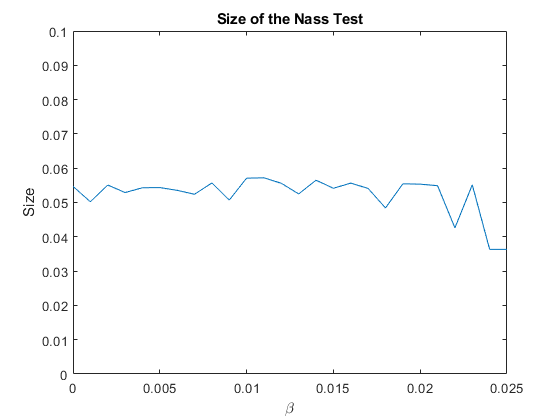
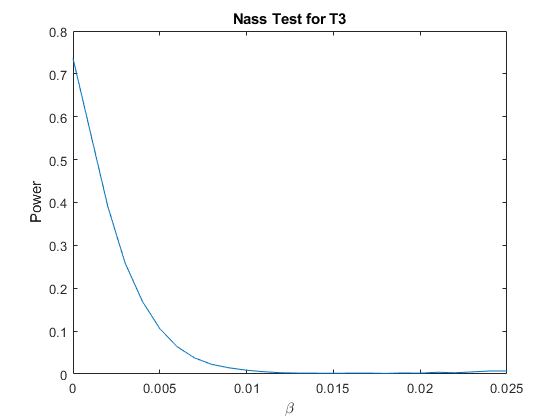
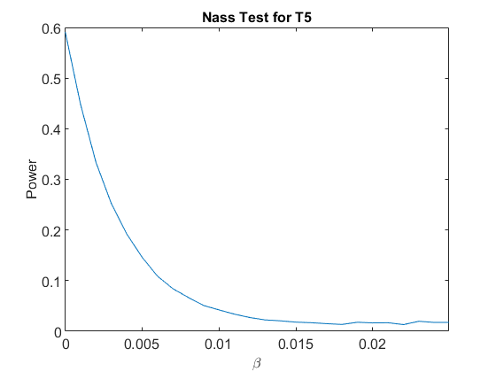
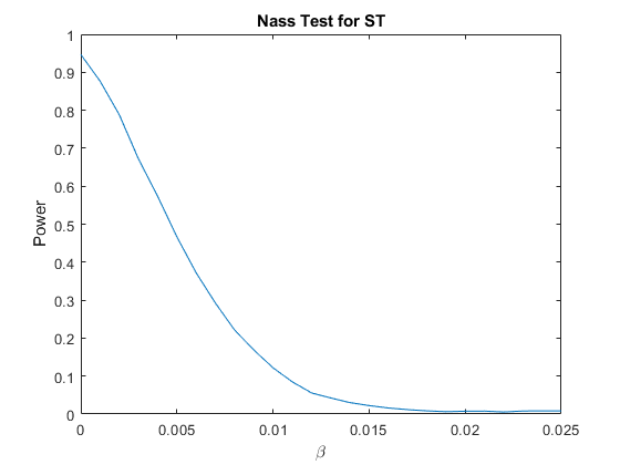
Figure 2: Size and Power for the RV@R approaching the AV@R at level $0.025$

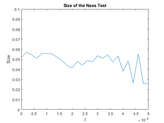
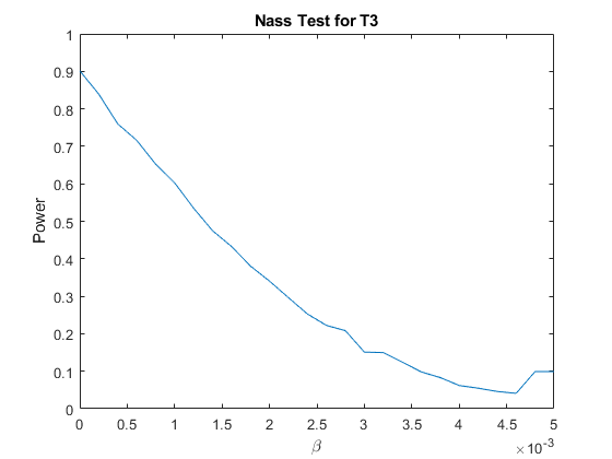
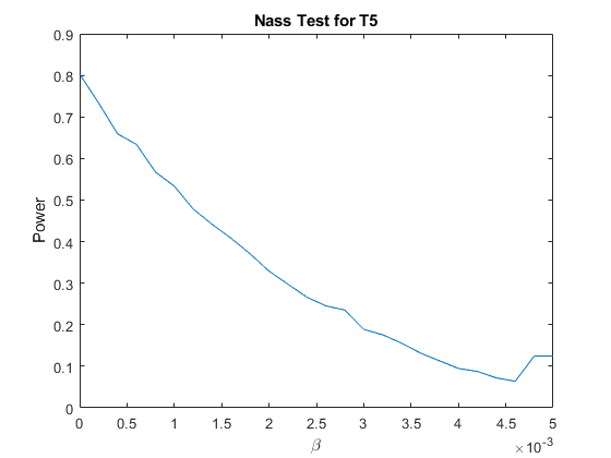
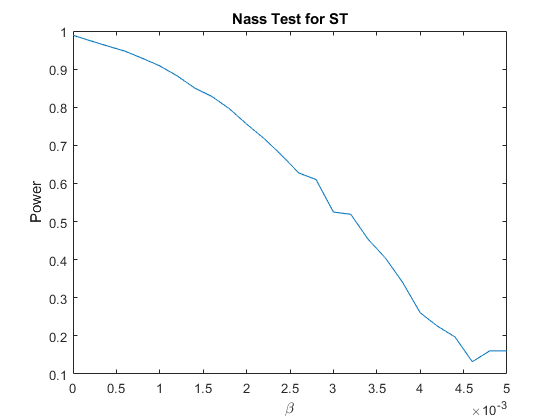
Figure 3: Size and Power for the RV@R approaching the AV@R at level $0.005$

RV@R is a distortion risk measure with distortion function $g(u)=\frac{u-\beta}{\alpha-\beta}\mathds{1}_{\{\beta<u\leq\alpha\}}+\mathds{1}_{\{u>\alpha\}}$, $0<\beta<\alpha$. This risk measure ignores the tail beyond the value at risk at level $\alpha$ and is therefore – just as the value at risk – not sensitive to extreme events. In the limiting case $\beta\to 0$, it coincides with tail-sensitive $AV@R_{\alpha}$. We repeat the case studies of Section 4 for $RV@R$. The results of the backtests are shown in Tables 7, 8 & 9 for $\alpha=0.025$, $\beta\in\{0.015,0.005,0.001\}$ and sample size $N=20000$. We use the partition $0=\alpha_{0}$, $\alpha_{i}=\beta+(\alpha-\beta)i/(m+1)$ for $i\in\{1,\dots,m\}$, and $\alpha_{m+1}=1$, and use otherwise the same backtesting strategy as for $AV@R$. The size of the asymptotic tests is in all cases reasonable. The power is generally poor for $\beta=0.015$ and improves, when smaller values of $\beta$ are chosen. This is due to the fact that for decreasing $\beta$ the risk measures $RV@R$ depends on more extreme parts of the tail. This is also apparent from Figure 2 where we plot the size of the test and the power for the three considered alternatives a function of $\beta$ in the case $m=16$, $n=1000$. The size is quite reasonable for all values of $\beta$, but the power is low unless $\beta$ is very close to zero. It increases to acceptable levels as $\beta\to 0$ from above, i.e., when approaching the limiting case $AV@R_{\alpha}$. A similar behavior holds also for other levels of $\alpha$; this is displayed in Figures 3 & 4 for $\alpha=0.5\%$ and $\alpha=10\%$, respectively.

The numerical experiments in Tables 7, 8 & 9 for $\alpha=0.025$, $\beta\in\{0.015,0.005,0.001\}$ were also repeated by us for the non-randomized method suggested in Kratz et al. (2018). The comparison showed again that our randomized method generally improves the power, while retaining a similar size. For $\beta=0.015$, the power is low for both methods and quite similar in most cases. For $\beta\in\{0.005,0.001\}$, the power improves. Im particular, for large $n$ and $m=2,4$ the randomized method performes best as well as better than Kratz et al. (2018). As an example, we include the detailed comparison for $\beta=0.005$ in Table 10.

Nass
$L_{t}$	$n|m$	1	2	4	8	16	32	64
$\mathcal{N}$	250	$0.89$	$0.75$	$1.20$	$0.98$	$0.99$	$0.87$	$1.26$
	500	$0.84$	$0.97$	$0.87$	$0.97$	$1.06$	$1.04$	$0.88$
	1000	$0.88$	$0.92$	$0.94$	$1.06$	$1.03$	$1.10$	$1.08$
	2000	$0.96$	$0.97$	$0.97$	$0.98$	$1.04$	$1.11$	$1.03$
T3	250	$1.68$	$1.65$	$1.36$	$0.57$	$0.40$	$0.32$	$0.46$
	500	$3.17$	$1.97$	$0.78$	$0.40$	$0.24$	$0.26$	$0.14$
	1000	$6.48$	$4.32$	$1.49$	$0.38$	$0.12$	$0.07$	$0.06$
	2000	$21.70$	$20.51$	$9.90$	$1.91$	$0.17$	$0.04$	$0.03$
T5	250	$4.96$	$4.21$	$3.81$	$2.29$	$2.03$	$1.80$	$2.08$
	500	$6.46$	$6.17$	$3.49$	$2.38$	$1.81$	$1.54$	$1.04$
	1000	$10.62$	$9.39$	$6.16$	$3.38$	$2$	$1.18$	$0.95$
	2000	$19.98$	$18.61$	$13.33$	$7.34$	$2.94$	$1.17$	$0.57$
ST	250	$7.46$	$6.68$	$4.29$	$1.47$	$0.95$	$0.75$	$0.78$
	500	$13.13$	$11.37$	$6.12$	$2.83$	$1.09$	$0.71$	$0.36$
	1000	$26.51$	$24.41$	$16.48$	$7.76$	$2.19$	$0.64$	$0.17$
	2000	$53.41$	$53.58$	$44.59$	$27.66$	$9.49$	$1.36$	$0.17$

Table 7: Backtesting $RV@R$ with $\beta=0.015$ and $\alpha=0.025$: Estimated size (for hypothesis $H_{0}$ with distribution $\mathcal{N}$) and power in $\%$ (for the alternatives $H_{1}$ with distributions $T3$, $T5$, $ST$, respectively) for the Pearson test, Nass test and LRT. The size is represented as the fraction of the true size according to our simulations divided by the desired level $\kappa=5\%$. The colouring scheme for the size is as follows: Values between $0.8-1.2$ are green, values between $0.9-1.1$ are dark green; values above $1.5$ are red, above $2$ dark red. The colouring scheme for the power is adopted from Kratz et al. (2018): Green refers to a power $\geq 70\%$; light red indicates a power $\leq 30\%$; dark red indicates poor results with a power $\leq 10\%$.

Nass
$L_{t}$	$n|m$	1	2	4	8	16	32	64
$\mathcal{N}$	250	$0.71$	$0.90$	$0.86$	$0.98$	$1.14$	$1.06$	$0.88$
	500	$0.85$	$0.96$	$0.89$	$1.10$	$1.08$	$1.11$	$1.08$
	1000	$0.98$	$0.95$	$0.90$	$1.04$	$1.08$	$1.10$	$1.12$
	2000	$0.98$	$0.95$	$0.98$	$1$	$1.06$	$1.07$	$1.12$
T3	250	$7.49$	$9.01$	$6.99$	$4.21$	$1.57$	$0.66$	$0.26$
	500	$15.55$	$16.54$	$13.44$	$8.24$	$3.33$	$0.75$	$0.18$
	1000	$35.82$	$38.16$	$35.91$	$24.43$	$10.32$	$2.33$	$0.27$
	2000	$68.38$	$76.86$	$78.44$	$67.86$	$43.69$	$14.09$	$1.44$
T5	250	$10.27$	$11.76$	$8.94$	$6.97$	$4.32$	$2.73$	$2.06$
	500	$17.80$	$17.92$	$15.22$	$11.84$	$7.03$	$3.43$	$2.07$
	1000	$32.11$	$32.20$	$30.80$	$23.69$	$14.71$	$6.34$	$2.58$
	2000	$54.40$	$59.11$	$58.86$	$50.96$	$37.52$	$19.02$	$6.39$
ST	250	$21.31$	$23.41$	$19.40$	$13.94$	$6.83$	$2.64$	$1.17$
	500	$39.52$	$42.03$	$38.82$	$30.55$	$17.89$	$6.57$	$1.63$
	1000	$69.27$	$72.11$	$71.50$	$64.32$	$46.04$	$23.13$	$6$
	2000	$93.38$	$96.14$	$96.59$	$94.72$	$88.51$	$69.92$	$32.97$

Table 8: Backtesting $RV@R$ with $\beta=0.005$ and $\alpha=0.025$: Estimated size (for hypothesis $H_{0}$ with distribution $\mathcal{N}$) and power in $\%$ (for the alternatives $H_{1}$ with distributions $T3$, $T5$, $ST$, respectively) for the Pearson test, Nass test and LRT. The size is represented as the fraction of the true size according to our simulations divided by the desired level $\kappa=5\%$. The colouring scheme for the size is as follows: Values between $0.8-1.2$ are green, values between $0.9-1.1$ are dark green; values above $1.5$ are red, above $2$ dark red. The colouring scheme for the power is adopted from Kratz et al. (2018): Green refers to a power $\geq 70\%$; light red indicates a power $\leq 30\%$; dark red indicates poor results with a power $\leq 10\%$.

Nass
$L_{t}$	$n|m$	1	2	4	8	16	32	64
$\mathcal{N}$	250	$0.74$	$0.99$	$1.04$	$1.09$	$1.09$	$1.04$	$0.91$
	500	$0.79$	$0.90$	$1.04$	$1.03$	$1.05$	$1.04$	$1.01$
	1000	$0.86$	$0.95$	$0.98$	$1.06$	$1.04$	$1.09$	$1.08$
	2000	$0.99$	$0.97$	$0.96$	$1.04$	$1.05$	$1.09$	$1.11$
T3	250	$12.14$	$18.22$	$19.82$	$16$	$13.33$	$6.71$	$2.60$
	500	$24.55$	$31.22$	$34.09$	$32.98$	$24.34$	$16.74$	$6.12$
	1000	$48.77$	$62.13$	$65.91$	$64.52$	$55.48$	$39.21$	$19.71$
	2000	$82.67$	$91.71$	$94.80$	$95.10$	$91.81$	$81.75$	$58.79$
T5	250	$14.62$	$17.46$	$19.05$	$16.11$	$12.88$	$9.62$	$5.31$
	500	$23.34$	$28.62$	$30.15$	$28.05$	$23.26$	$16.82$	$9.05$
	1000	$40.33$	$47.04$	$51.19$	$50.85$	$45.08$	$34.89$	$20.55$
	2000	$67.08$	$76.53$	$81.26$	$81.16$	$77.37$	$67.37$	$50.02$
ST	250	$29.59$	$35.95$	$39.63$	$36.11$	$31.47$	$21.02$	$10.08$
	500	$51.02$	$59.44$	$63.81$	$62.87$	$55.77$	$45.35$	$27.75$
	1000	$80.22$	$86.84$	$90.03$	$90.38$	$87.37$	$79.75$	$63.28$
	2000	$97.76$	$99.28$	$99.60$	$99.76$	$99.56$	$98.81$	$95.99$

Table 9: Backtesting $RV@R$ with $\beta=0.001$ and $\alpha=0.025$: Estimated size (for hypothesis $H_{0}$ with distribution $\mathcal{N}$) and power in $\%$ (for the alternatives $H_{1}$ with distributions $T3$, $T5$, $ST$, respectively) for the Pearson test, Nass test and LRT. The size is represented as the fraction of the true size according to our simulations divided by the desired level $\kappa=5\%$. The colouring scheme for the size is as follows: Values between $0.8-1.2$ are green, values between $0.9-1.1$ are dark green; values above $1.5$ are red, above $2$ dark red. The colouring scheme for the power is adopted from Kratz et al. (2018): Green refers to a power $\geq 70\%$; light red indicates a power $\leq 30\%$; dark red indicates poor results with a power $\leq 10\%$.

Nass
$L_{t}$	$n|m$	1	2	4	8	16	32	64
$\mathcal{N}$	250	$0.74$	$0.92$	$1.05$	$0.89$	$1.08$	$1.08$	$0.90$
	500	$1.18$	$0.90$	$0.98$	$1.07$	$1.10$	$1.10$	$1.06$
	1000	$0.94$	$0.98$	$0.92$	$0.97$	$1.07$	$1.09$	$1.02$
	2000	$1.05$	$0.90$	$0.94$	$0.99$	$1.03$	$1.07$	$1.09$
T3	250	$1.91$	$2.95$	$0.94$	$0.72$	$0.03$	$0.01$	$0.02$
	500	$7.02$	$5.10$	$4.04$	$2.05$	$0.66$	$0.11$	$0.03$
	1000	$28.51$	$19.27$	$11.13$	$5.38$	$1.59$	$0.46$	$0.04$
	2000	$57.49$	$30.93$	$15.93$	$10.05$	$6.55$	$2.05$	$-0.05$
T5	250	$-0.54$	$2.37$	$0.37$	$0.45$	$-0.03$	$0.27$	$0.05$
	500	$0.93$	$2$	$2.92$	$1.67$	$0.32$	$0.27$	$0.03$
	1000	$10.97$	$7.56$	$5.56$	$2.52$	$1.24$	$0.16$	$0.07$
	2000	$21.63$	$14.92$	$10.96$	$6$	$2.70$	$1.11$	$0.43$
ST	250	$3.18$	$6.53$	$1.45$	$1.31$	$0.19$	$0.16$	$0.12$
	500	$10.53$	$8.16$	$8.03$	$4.55$	$2.06$	$-0.05$	$-0.27$
	1000	$26.54$	$15.32$	$9.70$	$6.60$	$3.69$	$1.21$	$0.91$
	2000	$25.50$	$9.30$	$4.29$	$2.86$	$3.18$	$2.96$	$0.99$

Table 10: Backtesting $RV@R$: Comparison of the results in Table 8 to the method of Kratz et al. (2018). The size is represented as the fraction of the true size according to our simulations divided by the desired level $\kappa=5\%$. The colouring scheme for the size is as follows: Values between $0.8-1.2$ are dark green, values between $0.9-1.1$ are dark green; values above $1.5$ are red, above $2$ dark red. For the alternative $T3$, $T5$ and $ST$ , the table shows the difference of the power of our method and the method of KLM. The colouring scheme for the power is as follows: Dark green are notable improvements of the power $\geq 20\%$; light green are improvements $\geq 10\%$.

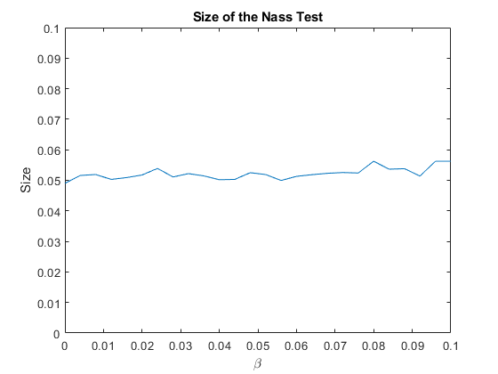
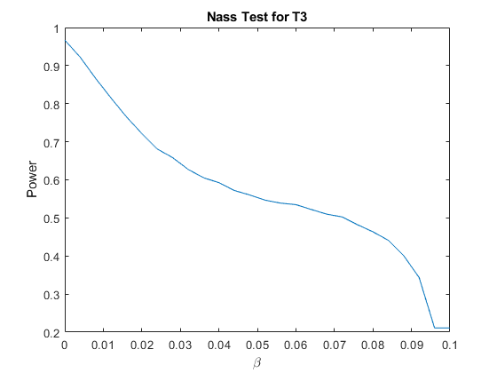
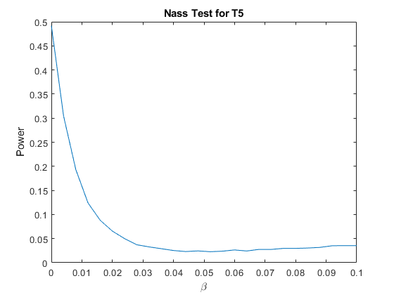
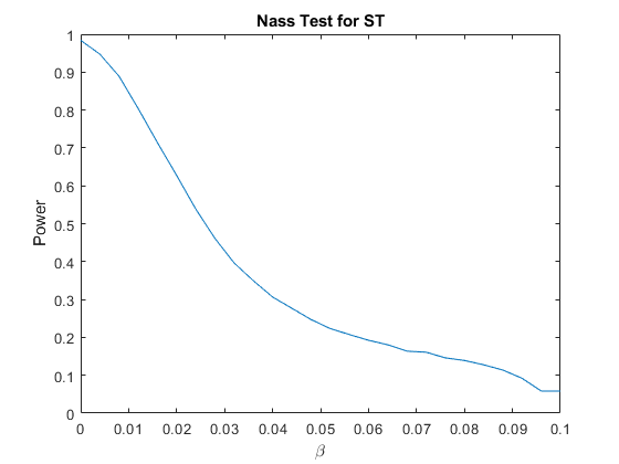
Figure 4: Size and Power for the RV@R approaching the AV@R at level $0.1$

A.10 S&P 500

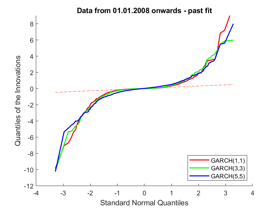
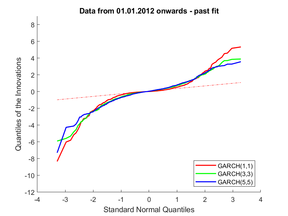
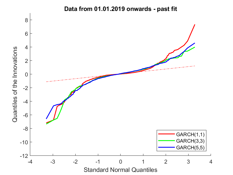
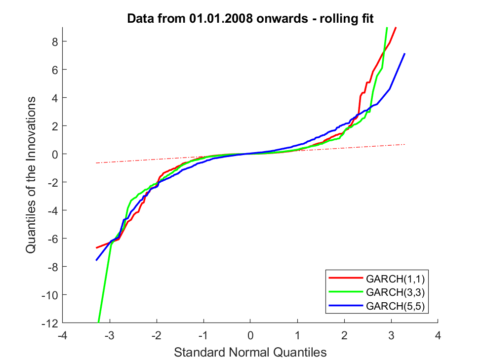
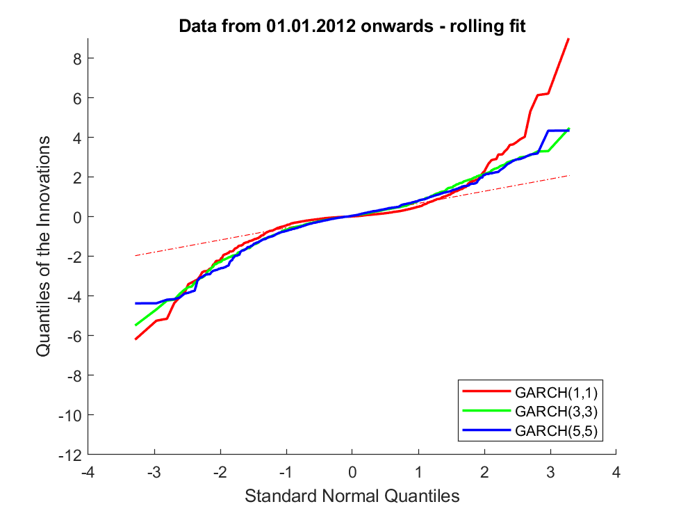
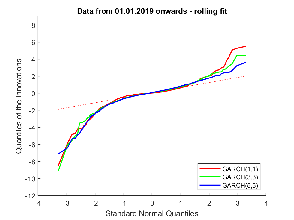
Figure 5: QQ-plots of the standard normal distributions and the normalized innovations of the fitted GARCH models to the S&P 500. The GARCH models are fitted on $500$ data points and the innovations are observed for the following $1000$ data points.

We investigate the power of the backtests for log returns of the S&P 500 during three different time periods, starting at the beginning of the years 2008, 2012 and 2019, respectively. Since we are focussing on losses, we consider the negative of the log returns, i.e., downside risk measures are statistical functionals of the upper tail of the corresponding distributions.

The exemplary time series models used are GARCH processes with standard normal innovations $GARCH(p,q)$ with $p=q$ and $p=1,3,5$. The model classes are nested; larger $p$ corresponds to a larger class and higher complexity. We consider two different methodologies to fit the models and to apply our backtesting procedure. The first approach fits the GARCH-processes to the first 250 resp. 500 data points. The backtest is then applied to the 1000 following observations of the processes. The second approach does not assume that the true data-generating mechanism is a GARCH-process with constant parameters, but refits the processes at each point of time based on the latest 250 resp. 500 data points to produce a model for the next innovation. Again 1000 observations are used for the backtest.

QQ-plots demonstrate that innovations are not Gaussian and that the models are misspecified. We illustrate this for fits based on 500 data points in Figure 5. The deviations from normality in the upper tail are of different size when varying the time period, model, and fitting methodology. Risk measures backtests capture the importance of these discrepancies in terms of specific functionals of the downside risk. All fitted GARCH processes satisfy Bollerslev’s condition for weak stationarity, cf. Bollerslev (1986), or also Lindner (2009) for a concise survey of stationarity conditions.

We consider $AV@R$ and $GlueV@R$ with the same parameters as before. The probabilities of rejection (corresponding to the power) is estimated in $2000$ runs of the backtest for $m=8$ and a partition $\alpha_{0}<\alpha_{1}<\dots<\alpha_{m}<\alpha_{m+1}=1$ such that $\alpha_{i}=i/(m+1)\cdot\alpha$, $i\in\{1,\dots,m\}$.

Nass
	01.01.2008		01.01.2012		01.01.2019
Model / Fit	$250$	$500$	$250$	$500$	$250$	$500$
$GARCH(1,1)$	$1$	$1$	$1$	$1$	$1$	$1$
$GARCH(3,3)$	$1$	$1$	$1$	$0.13$	$0.28$	$1$
$GARCH(5,5)$	$1$	$1$	$0$	$0.07$	$0.03$	$0$

Table 11: Rejection probabilities of the backtest on log returns of the S&P500 versus GARCH models fitted on past observations from a fixed time point with respect to the $AV@R_{0.975}$.

Nass
	01.01.2008		01.01.2012		01.01.2019
Model / Fit	$250$	$500$	$250$	$500$	$250$	$500$
$GARCH(1,1)$	$1$	$1$	$1$	$1$	$1$	$1$
$GARCH(3,3)$	$1$	$1$	$1$	$1$	$0.09$	$0.48$
$GARCH(5,5)$	$1$	$1$	$1$	$1$	$0.67$	$0$

Table 12: Rejection probabilities of the backtest on log returns of the S&P500 versus GARCH models fitted with a rolling collection of observations with respect to the $AV@R_{0.975}$.

Nass
	01.01.2008		01.01.2012		01.01.2019
Model / Fit	$250$	$500$	$250$	$500$	$250$	$500$
$GARCH(1,1)$	$1$	$1$	$1$	$1$	$1$	$1$
$GARCH(3,3)$	$1$	$1$	$0.87$	$0.07$	$0.01$	$1$
$GARCH(5,5)$	$1$	$1$	$0$	$0$	$0$	$0$

Table 13: Rejection probabilities of the backtest on log returns of the S&P500 versus GARCH models fitted on past observations from a fixed time point with respect to the $GlueV@R^{h_{1},h_{2}}_{\beta,\alpha}$, where $h_{1}=2/5$, $h_{2}=2/3$, $\alpha=0.05$, $\beta=0.01$.

Nass
	01.01.2008		01.01.2012		01.01.2019
Model / Fit	$250$	$500$	$250$	$500$	$250$	$500$
$GARCH(1,1)$	$1$	$1$	$1$	$1$	$1$	$1$
$GARCH(3,3)$	$1$	$1$	$1$	$1$	$1$	$1$
$GARCH(5,5)$	$1$	$1$	$1$	$1$	$1$	$1$

Table 14: Rejection probabilities of the backtest on log returns of the S&P500 versus GARCH models fitted with a rolling collection of observations with respect to the $GlueV@R^{h_{1},h_{2}}_{\beta,\alpha}$, where $h_{1}=2/5$, $h_{2}=2/3$, $\alpha=0.05$, $\beta=0.01$.

Tables 14, 14, 14 & 14 show in most cases the null hypothesis is rejected, especially always during the financial crisis corresponding to the time period starting at 2008. Only during the other periods for $p\geq 3$ rejection probabilities are low in some cases corresponding to smaller deviations from normality in the upper tail. The differences between the two fitting methods make misspecification even more apparent.

Nass
$L_{t}$	$n|m$	1	2	4	8	16	32	64
Size	250	$1.11$	$1.47$	$1.20$	$1.07$	$1.07$	$1.18$	$1.11$
	500	$1.68$	$1.36$	$1.25$	$1.19$	$1.26$	$1.21$	$1.21$
	1000	$1.73$	$1.54$	$1.35$	$1.21$	$1.20$	$1.17$	$1.06$
	2000	$1.90$	$1.35$	$1.28$	$1.18$	$1.16$	$1.21$	$1.18$
NB	250	$66.60$	$65.23$	$63.64$	$62.22$	$58.74$	$58.74$	$59.65$
	500	$87.85$	$88.07$	$84.25$	$83.95$	$81.84$	$79.24$	$81.95$
	1000	$98.82$	$98.87$	$98.30$	$98$	$96.69$	$96.24$	$95.89$
	2000	$99.98$	$99.99$	$99.99$	$99.98$	$99.96$	$99.93$	$99.81$
PAR	250	$95.40$	$97.19$	$98.29$	$98.04$	$97.64$	$97.59$	$96.92$
	500	$99.86$	$100$	$99.94$	$99.94$	$99.98$	$99.96$	$99.96$
	1000	$100$	$100$	$100$	$100$	$100$	$100$	$100$
	2000	$100$	$100$	$100$	$100$	$100$	$100$	$100$
LOGN	250	$46.91$	$49.27$	$49.89$	$47.54$	$46.90$	$46.55$	$44.87$
	500	$72.78$	$69.83$	$70.99$	$69.46$	$69.24$	$70.11$	$67.91$
	1000	$91.83$	$92.73$	$92.77$	$92.04$	$91.53$	$90.53$	$89.30$
	2000	$99.50$	$99.68$	$99.62$	$99.68$	$99.50$	$99.50$	$99.05$

Table 15: ALM Backtest for $AV@R_{\alpha}$ with $\alpha=0.05$. The size is represented as fraction of estimated size divided by the desired level $\kappa=0.05$. Values of the size between $0.9-1.1$ are dark green, between $0.8-1.2$ are light green, above $1.5$ are red and above $2$ dark red. For the power green refers to a power $\geq 70\%$; light red to a power $\leq 30\%$ and dark red indicates a power $\leq 10\%$.

A.11 Some Further Results in the Context of ALM

.

We repeat the case studies for $AV@R$. The parameters are chosen as in the $GlueV@R$-ALM simulation, and the partition for the risk measure test statistics is set as in the distribution simulations. Qualitatively the results are similar as for $GlueV@R$ and shown in Table 15.

Since the true size of the test deviates from the a priori targeted level, since its construction is based on asymptotic results, we construct alternative tests which are not based on the target size $0.05$ but on a smaller size $\kappa=0.025$ at the expense of deterioration of the power. This is displayed in Tables 16 & 17. The realized size is in most case smaller than the targeted size, and also the power of the tests not reduced by a large amount. The strategy of using a smaller than target size for the asymptotic construction appears to be a viable method.

Nass
$L_{t}$	$n|m$	1	2	4	8	16	32	64
Size	250	$0.57$	$0.91$	$0.93$	$0.62$	$0.60$	$0.72$	$0.57$
	500	$1.12$	$0.85$	$0.68$	$0.66$	$0.68$	$0.74$	$0.67$
	1000	$1.22$	$0.89$	$0.82$	$0.70$	$0.62$	$0.65$	$0.72$
	2000	$1.24$	$0.95$	$0.75$	$0.65$	$0.69$	$0.59$	$0.67$
NB	250	$60.81$	$56.89$	$55.63$	$54$	$50.71$	$49.48$	$49.31$
	500	$86.17$	$85.37$	$79.84$	$78.95$	$75.99$	$72.64$	$75.97$
	1000	$98.29$	$98.09$	$97.40$	$96.61$	$94.81$	$94.31$	$93.30$
	2000	$99.99$	$99.98$	$99.98$	$99.95$	$99.92$	$99.83$	$99.64$
PAR	250	$93.59$	$95.62$	$97.34$	$97.08$	$97.04$	$96.99$	$95.84$
	500	$99.83$	$99.91$	$99.88$	$99.93$	$99.94$	$99.93$	$99.92$
	1000	$100$	$100$	$100$	$100$	$100$	$100$	$100$
	2000	$100$	$100$	$100$	$100$	$100$	$100$	$100$
LOGN	250	$40.21$	$39.43$	$43.04$	$40.07$	$38.90$	$38.12$	$36.79$
	500	$66.71$	$65.37$	$64.89$	$63.40$	$62.49$	$61.93$	$60.08$
	1000	$89.83$	$89.96$	$89.24$	$88.46$	$88.86$	$87.85$	$86$
	2000	$99.15$	$99.24$	$99.24$	$99.43$	$99.03$	$99.22$	$98.66$

Table 16: ALM Backtest for $AV@R_{\alpha}$ with $\alpha=0.05$. The level of the tests is set to $\kappa=0.025$. The estimated size is represented as fraction to $0.05$. Values of the size between $0.9-1.1$ are dark blue, between $0.8-1.2$ are light blue. For the power green refers to a power $\geq 70\%$; light red to a power $\leq 30\%$ and dark red indicates a power $\leq 10\%$.

Nass
$L_{t}$	$n|m$	1	2	4	8	16	32	64
Size	250	$1.08$	$0.99$	$0.95$	$0.69$	$0.66$	$0.74$	$0.53$
	500	$1.03$	$0.79$	$0.69$	$0.67$	$0.69$	$0.62$	$0.63$
	1000	$1.17$	$0.93$	$0.71$	$0.66$	$0.66$	$0.63$	$0.75$
	2000	$1.33$	$0.92$	$0.74$	$0.68$	$0.68$	$0.57$	$0.71$
NB	250	$58.97$	$60.05$	$56.49$	$54.13$	$49.21$	$49.72$	$49.94$
	500	$86.05$	$86.23$	$79.43$	$78.97$	$76.74$	$72.93$	$75.03$
	1000	$98.79$	$98.37$	$97.97$	$96.91$	$94.86$	$94.55$	$93.93$
	2000	$99.98$	$99.97$	$99.97$	$99.93$	$99.90$	$99.86$	$99.72$
PAR	250	$94.68$	$98.03$	$97.40$	$96.81$	$96.69$	$96.80$	$96.26$
	500	$99.95$	$99.96$	$99.89$	$99.94$	$99.94$	$99.94$	$99.90$
	1000	$100$	$100$	$100$	$100$	$100$	$100$	$100$
	2000	$100$	$100$	$100$	$100$	$100$	$100$	$100$
LOGN	250	$40.75$	$45.98$	$43.49$	$40.20$	$38.59$	$38.37$	$36.38$
	500	$69.05$	$67.28$	$64.63$	$63.81$	$62.54$	$62.07$	$59.76$
	1000	$91.99$	$91.47$	$89.80$	$89.11$	$87.65$	$86.83$	$85.32$
	2000	$99.51$	$99.60$	$99.19$	$99.41$	$99.25$	$98.96$	$98.84$

Table 17: ALM Backtest for the $GlueV@R$ with $h_{1}=2/5$, $h_{2}=2/3$, $\alpha=0.05$, $\beta=0.01$. he level of the tests is set to $\kappa=0.025$. The estimated size is represented as fraction to $0.05$. Values of the size between $0.9-1.1$ are dark blue, between $0.8-1.2$ are light blue. For the power green refers to a power $\geq 70\%$; light red to a power $\leq 30\%$ and dark red indicates a power $\leq 10\%$.

References

- Acerbi (2002) Carlo Acerbi. Spectral measures of risk: A coherent representation of subjective risk aversion. Journal of Banking & Finance, 26(7):1505–1518, 2002.
- Acerbi and Szekely (2014) Carlo Acerbi and Balazs Szekely. Back-testing Expected Shortfall. Risk, 27(11):76–81, 2014.
- Artzner et al. (1999) Philippe Artzner, Freddy Delbaen, Jean-Marc Eber, and David Heath. Coherent measures of risk. Mathematical finance, 9(3):203–228, 1999.
- Balbás et al. (2009) Alejandro Balbás, José Garrido, and Silvia Mayoral. Properties of distortion risk measures. Methodology and Computing in Applied Probability, 11(3):385, 2009.