Abstract
We revisit the recipe for hadron formation in the Lund string hadronization model. Given an incoming quark or quark-diquark pair, weights for hadron formation are updated to take hyperfine splitting effects arising from the mass difference between $\mathrm{u,d}$-type and $\mathrm{s}$-type quarks. We find that the procedure improves the description of hadron yields in $\mathrm{e}^{+}\mathrm{e}^{-}$ collisions and the $\phi$ cross section in neutral current DIS. We also show results for proton collisions, and discuss the future use of this study in the context of small system collectivity.

dummy

1 Introduction

The surprising discovery from LHC [1] of continuous strangeness enhancement with final state multiplicity across collision systems, has spurred a renewed interest in hadronization models. While increased strangeness production in heavy ion collisions is traditionally seen as a signature of Quark–Gluon Plasma (QGP) formation [2, 3, 4], microscopic hadronization models such as the Lund string model [5] or the cluster model [6] can describe similar effects using models of cluster reconnections [7, 8] or string interactions, such as rope formation [9, 10] or junction formation [11, 10]. In the case of junction formation, even more attention has been gathered by the observation that also charm baryon yields are enhanced in hadronic collisions compared to $\mathrm{e}^{+}\mathrm{e}^{-}$ [12].

What all these approaches have in common, is their connection to the LEP baseline. As the basic notion of the models is that of jet universality, i.e. that the same physics model should hold in all collision systems, parameters are often estimated using data from $\mathrm{e}^{+}\mathrm{e}^{-}$ collisions at the $\mathrm{Z}$ pole [13]. This, in turn, means that no model attempting to describe features of pp collisions, will perform better than the LEP baseline. And while e.g. the Lund model as implemented in the P YTHIA Monte Carlo event generator [14] does a reasonable job at describing the data, there are still details less well described, even total yields of some of the most intensely studied baryon and meson species in proton collisions, such as the $\phi$ meson and $\Omega^{-}$ baryon, both characterized by having the maximal amount of inner strangeness.

Several tunes for the P YTHIA event generator have been presented, as new experimental results have been available; the present default tune in P YTHIA 8 is the ”Monash tune” from 2014 [13]. However, the basic parametrization is not changed at least since JETSET 6.2 in 1986 [15].

The production of different hadrons depends both on their quark content and the hadron mass. As discussed in section 2, the string can break via $q\bar{q}$ pair production in a kind of tunnelling process [16]. Here the virtual quark and antiquark are regarded as produced in a single point and pulled apart by the string tension until they come on shell, and the result is a Gaussian suppression for higher quark masses.

The production probability also depends on the mass of the hadron, which is sensitive to the spin-spin interaction between two quarks, proportional to $\mathbf{M}_{1}\cdot\mathbf{M}_{2}$, where $M_{i}\propto g/\mu_{i}$ are the magnetic moments and $\mu_{i}$ the masses of the quark and the antiquark in a meson, or in any pair of two quarks in a baryon. This effect separates the mass of the $\rho$-meson and the pion, leading to a suppression of the $\rho/\pi$ ratio by about a factor 1/2 (on top of the factor 3 from spin counting). Due to the larger mass of the strange quark the mass difference between K^∗ and K is smaller, and the K^∗/K similarly less suppressed. However, lacking experimental information at the time, the interaction between two strange quarks in an ss diquark in a baryon, or in an $\mathrm{s\bar{s}}$ pair in a $\phi$ meson, did not get a corresponding extra reduced suppression, beyond the suppression from a single s-quark. (The $\eta$ and $\eta^{\prime}$ mesons, both with a significant $\mathrm{s\bar{s}}$ content and with very low production rates, got their individual tunable suppression factors fitted to data; see also the discussion in ref. [17].) In section 3 below, we present a relatively simple way to take the modified spin interaction between two strange quarks into account. It is most important for multi-strange baryons, but it has also a non-negligible effect on the production of $\phi$ mesons. The lower suppression of multi-strange baryons will also imply a larger suppression for $\Delta^{++}$.

In the following we will first recap the basic features of string hadronization in section 2, before we introduce the improvements concerning the strange quarks in section 3. A tune to the modified hadronization is presented in section 4. We present some result in section 5, noting that the majority of results presented here are either for $\mathrm{e}^{+}\mathrm{e}^{-}$ collisions or low-multiplicity proton collisions, in order to compare to an environment as free as possible from effects from rope hadronization, junction formation etc. Finally in section 6 we present our conclusions.

2 Lund string fragmentation

We will here discuss the basics of the Lund string hadronization model as implemented in P YTHIA ; for more details see ref. [5]. In the model the confining colour field is approximated by a “massless relativistic string”. (For the dynamics of such a string we refer to ref. [18].) A straight string is invariant under longitudinal boosts, with a given energy per unit length (or tension) $\kappa\approx 1$ GeV/fm, but no longitudinal momentum. It can be visualised as a thin tube with a homogeneous electric field, similar to a vortex line in a superconductor (with electric and magnetic fields exchanged).

The string can break by the production of a $\mathrm{q}\bar{\mathrm{q}}$ pair, in a process analogous to the production of $\mathrm{e}^{+}\mathrm{e}^{-}$ pairs in a homogeneous electric field. This gives [19]:

$$\exp(-\pi(\mu^{2}+p_{\perp}^{2})/\kappa)=\exp(-\pi\mu^{2}/\kappa)\times\exp(-\pi p_{\perp}^{2}/\kappa),$$ (1)

where $\mu$ and $p_{\perp}$ are the mass and transverse momentum for the quark and anti-quark in the pair. The quark and anti-quark are then pulled in opposite directions by the string tension. The result in eq. (1) can also be regarded as a result of tunnelling, where the quark and antiquark are produced in a single point as virtual particles, and pulled apart a distance $2\sqrt{\mu^{2}+p_{\perp}^{2}}/\kappa$ until they can come on shell [16]. A quark and an anti-quark from neighbouring breakups can combine to form a meson, if the mass is correct.

Another important feature of the model is that a gluon is treated as a momentum carrying “kink” on the string, pulled back by the force $2\kappa$ from the two adjacent string pieces. The fragmentation of such a string with several intermediate gluons is discussed in ref. [20]. In this section we will, however, focus on the fragmentation of a straight string between a quark and an antiquark, without intermediate gluons.

2.1 Meson production

2.1.1 Ideal case with a single meson species

For simplicity we first limit ourself to the situation with a single hadron species, neglecting also transverse momenta. In this simplified situation the breakup to a state with $n$ hadrons is given by the expression [21]:

$$d\mathcal{P}\propto\prod_{i=1}^{n}\left[Nd^{2}p_{i}\delta(p^{2}_{i}-m^{2})\right]\delta^{(2)}\!\left(\sum p_{i}-P_{\mathrm{tot}}\right)\exp\left(-bA\right).$$ (2)

Here $p_{i}$ (with $i=1,...,n$) and $P_{\mathrm{tot}}$ are two-dimensional vectors. The expression is a product of a phase space factor, where the parameter $N$ expresses the ratio between the phase space for $n$ and $n-1$ particles, and the exponent of the imaginary part of the string action, $bA$. Here $b$ is a parameter and $A$ the space–time area covered by the string before breakup (in units of the string tension $\kappa$). This decay law can (for large enough energies) be implemented as an iterative process, where each successive hadron takes a fraction $z$ of the remaining light-cone momentum ($p^{\pm}=E\pm p_{z}$) along the positive or negative light-cone, depending on from which end the hadron is ”peeled off”. The values of these momentum fractions are then given by the distribution

$$f(z)=N\frac{(1-z)^{a}}{z}\exp(-bm^{2}/z).$$ (3)

Here $a$ is related to the parameters $N$ and $b$ in eq. (2) by normalization. (In practice $a$ and $b$ are determined from experiments, and $N$ is then determined by the normalization constraint.) The result in eq. (3) is in principle valid for strings stretched between partons produced in a single space–time point, and moving apart as illustrated in the space–time diagram in figure 1.

Figure 1: Breakup of a string between a quark and an anti-quark in a $x-t$ diagram. New $q\bar{q}$ pairs are produced around a hyperbola, and combine to the outgoing hadrons. The original $q$ and $\bar{q}$ move along light-like trajectories. The area enclosed by the quark lines is the coherence area $A$ in eq. (2), in units of the string tension $\kappa$.

The expression in eq. (2) is boost invariant, and the hadrons are produced around a hyperbola in space–time. A Lorentz boost in the $x$-direction will expand the figure in the $(t+x)$ direction and compress it in the $(t-x)$ direction (or vice versa). Thus the breakups will be lying along the same hyperbola, and low momentum particles in a specific frame will always be the first to be produced in that special frame. The typical proper time for the breakup points is given by

$$\langle\tau^{2}\rangle=\frac{1+a}{b\kappa^{2}}.$$ (4)

With parameters $a$ and $b$ determined by tuning to data from $\mathrm{e}^{+}\mathrm{e}^{-}$ annihilation at LEP, and $\kappa$ equal to 0.9-1 GeV/fm, eq. (4) gives a typical breakup time of 1.5 fm.

2.1.2 Flavour, transverse momentum, and spin

In practice it is also necessary to account for different quark and hadron species, and for quark transverse momenta. With $\kappa\approx$ 1 GeV/fm eq. (1) implies that strange quarks are suppressed by roughly a factor 0.3 relative to a u- or a d-quark. It also means that the quarks are produced with an average $p_{\perp}\sim 250$ MeV, independent of its flavour. When a u- and a $\bar{\mathrm{d}}$-quark from neighbouring breakups combine to form a meson, it can result in either a pion or a $\rho$-meson. As stated in the introduction, the relative probabilities depend on the number of available spin states, but also by the normalization of the meson wavefunction affected by the spin-spin interaction between the quarks. The latter is proportional to $\mathbf{M}_{1}\cdot\mathbf{M}_{2}$, where $M_{i}\propto g/\mu_{i}$ are the colour magnetic moments of the two components. As discussed in ref. [5], this can compensate the factor 3 from spin counting, giving a relative probability closer to 1, in agreement with observations [22, 13].

Of interest here is that the colour magnetic moment is proportional to $1/\mu$, where $\mu$ is the “effective” mass of the quark. Therefore this effect is smaller for hadrons with a strange quark, giving a $\mathrm{K}^{*}/\mathrm{K}$ ratio which is larger than the $\rho/\pi$ ratio. This effect was included already in early versions of P YTHIA . In conclusion the overall $q\bar{q}$ production rate is determined by the parameters $a$ and $b$ in eq. (3), and the relative rates for $\pi$, $\rho$, K, and K^∗, which are determined by three tuneable parameters, and which we for the purpose of this paper name as follows:

• The overall suppression of $\mathrm{s\bar{s}}$ string breaks relative to $\mathrm{u}$ or $\mathrm{d}$ ones. (In P YTHIA settings this parameter is called StringFlav:probStoUD, and has a default value of 0.217).

• The relative production ratio of vector mesons to pseudoscalar mesons for $\mathrm{u}$ or $\mathrm{d}$ types, not accounting for the factor 3 from spin counting. (In P YTHIA settings this parameter is called StringFlav:mesonUDvector, and has a default value of 0.50).

• The relative production ratio of vector mesons to pseudoscalar mesons for $\mathrm{s}$ types. (In P YTHIA settings this parameter is called StringFlav:mesonSvector, and has a default value of 0.55).

This implies that for e.g. a $\mathrm{u}\bar{\mathrm{d}}$ pair becomes a $\pi^{+}$ or a $\rho^{+}$ with the following probabilities (the factor 3 comes from spin counting):

$$P_{\pi}=1/(1+3y_{\mathrm{ud}});\,\,\,\,\,\,\,P_{\rho}=3y_{\mathrm{ud}}/(1+3y_{\mathrm{ud}}),$$ (5)

and similar probabilities for K and $\mathrm{K}^{*}$, with $y_{\mathrm{ud}}$ exchanged to $y_{\mathrm{s}}$.

The production of mesons with an $\mathrm{s}\bar{\mathrm{s}}$ pair is more complicated. For the isospin 0 vector mesons, $\phi$ is essentially a pure $\mathrm{s}\bar{\mathrm{s}}$ state, while $\omega$ contains only non-strange quarks. Thus we have $\omega=(\mathrm{u}\bar{\mathrm{u}}-\mathrm{d}\bar{\mathrm{d}})/\sqrt{2}$ (with the iso-triplet $\rho^{0}=(\mathrm{u}\bar{\mathrm{u}}+\mathrm{d}\bar{\mathrm{d}})/\sqrt{2}$). The $\omega$ mass is approximately the same as for $\rho$, and their production rates are also approximately the same. In default P YTHIA an $\mathrm{s}\bar{\mathrm{s}}$ pair will give a $\phi$ meson, with the same probability ($3y_{\mathrm{s}}/(1+3y_{\mathrm{s}})$) as a $\mathrm{K}^{*-}$ from an $\mathrm{s}\bar{\mathrm{u}}$ pair, although the $\phi$ has two strange quarks and K^∗ only one. In section 3.1 we discuss how we can take this difference into account.

The isospin 0 pseudoscalars, $\eta$ and $\eta^{\prime}$, are mixtures of the flavour singlet state $\eta_{1}=(\mathrm{u}\bar{\mathrm{u}}+\mathrm{d}\bar{\mathrm{d}}+\mathrm{s}\bar{\mathrm{s}})/\sqrt{3}$ and the octet state $\eta_{8}=(\mathrm{u}\bar{\mathrm{u}}+\mathrm{d}\bar{\mathrm{d}}-2\mathrm{s}\bar{\mathrm{s}})/\sqrt{6}$, with a mixing angle $\theta_{P}$ between -10 and -20 degrees:

$$\eta = \cos(\theta_{P})\,\eta_{8}-\sin(\theta_{P})\,\eta_{1},$$

$$\eta^{\prime} = \sin(\theta_{P})\,\eta_{8}+\cos(\theta_{P})\,\eta_{1}.$$ (6)

In a chiral symmetry limit, with all quarks being massless, $\eta_{8}$ would be a pseudo-Goldstone particle, along with the pion and the kaon. However, as both $\eta$ and $\eta^{\prime}$ are quite heavy, we are far from this limit. These particles also have quite low production rates. The solution in P YTHIA is to suppress them both with an individual tunable parameter. We note that this procedure makes the interpretation of the parameter $y_{\mathrm{s}}$ as the vector to pseudoscalar ratio ambiguous, as if no meson is chosen, a new trial break-up is made.

2.2 Baryon production

We here describe baryon production in a single string as realized in the “popcorn” model, which is the default treatment of baryon production in P YTHIA .

In analogy with the production of mesons in section 2.1, a baryon–antibaryon pair can be formed if the string breaks by the production of a diquark–antidiquark pair, forming a colour antitriplet and a triplet respectively [23]. In this case the $\mathrm{B}\bar{\mathrm{B}}$ pair will always have two quark flavours in common and lie close to each other in momentum space. Experimental data from $\mathrm{e}^{+}\mathrm{e}^{-}$ annihilation show that this is not always the case, and a model, with a stepwise production mechanism, called the popcorn model, was presented in ref. [24].

In a red–antired ($r\bar{r}$) string-field, a $b\bar{b}$ pair can be produced as a vacuum fluctuation. If the $r$ and $b$ charges form an antiblue antitriplet, then new $\mathrm{q}\bar{\mathrm{q}}$ pairs can be produced in the green string field. With a single such pair, the result would be similar to the diquark–antidiquark production described above. However, if more than one such pair is produced, we get not only a $\mathrm{B}\bar{\mathrm{B}}$ pair, but also one or more mesons in between them, as seen figure 2. In this case the baryon and the antibaryon may have only a single flavour in common. However, as the first $\mathrm{q}\bar{\mathrm{q}}$ pair (the blue pair above) is produced as a virtual fluctuation with limited lifetime, the production of several intermediate mesons, or the more massive vector mesons, is strongly suppressed. In the P YTHIA implementation therefore only a single intermediate meson is allowed, with the overestimated $\rho$ and $\omega$ mesons simulating the neglected combinations of two or three pions.

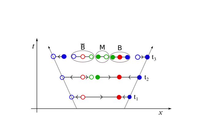
Figure 2: Illustration of the popcorn model with a string spanned between a blue and an antiblue charge. At $t_{1}$ a red-antired $q\bar{q}$ pair is produced as a virtual fluctuation. In the green field between then a two green-antigreen pairs are produced at $t_{2}$ and $t_{3}$. At $t_{3}$ also two new blue-antiblue pairs have been produced closer to the original blue and antiblue charges. The result is a baryon-antibaryon pair with a meson in between.

The default P YTHIA  implementation of diquark production, has three relevant parameters in addition to the suppression for every strange quark compared to non-strange quarks:

• suppression for a diquark compared to a single quark, independent of flavour and spin. (In P YTHIA settings this parameter is called StringFlav:probQQtoQ, and has a default value of 0.081).

• : extra suppression for diquarks with (any) strange content relative to diquarks without. (In P YTHIA settings this parameter is called StringFlav:probSQtoQQ, and has a default value of 0.915.) This suppression is in addition to the normal suppression due to the presence of an s-quark ($\rho$),

• suppression of spin 1 diquarks relative to spin 0 diquarks. (In P YTHIA settings this parameter is called StringFlav:probQQ1toQQ0, and has a default value of 0.0275.) This suppression comes on top of the factor 3 enhancement of vector diquarks from counting spin states.

The production rate of each (single) diquark can thus be calculated as the product of a spin factor, a vertex factor and a single-diquark tunnelling factor. These can in turn be combined for each possible diquark pair.

An essential feature here is that a baryon is an antisymmetric colour singlet state, and thus symmetric in flavour and spin. Therefore a diquark formed by two equal quarks can only have spin 1, and a ud-diquark must either have both spin and isospin 1, or both spin and isospin 0. The quark and diquark is then combined into a baryon, then again taking into account the total symmetry of the three-quark state. All relevant flavour information is determined by the parameters above, and in addition a baryon weight depending on the relevant SU(6) Clebsch-Gordan coefficients. As for the mesons, these may not necessarily add up to 1, and if no baryon is chosen a new trial is made.

3 Accounting for hyperfine splitting effects

As discussed in section 2 the production rate for different hadrons is affected by the spin interaction of the quarks. The spin-spin interaction between a quark and an anti-quark or between two quarks is proportional to the product of the two colour-magnetic moments, $\mathbf{M}_{1}\cdot\mathbf{M}_{2}$, which gives the ratio 3:(-1) between pairs with spin 1 and spin 0. As example this reduces the $\rho/\pi$ ratio from 3 (as given by spin counting) by approximately a factor 0.5. This effect is naturally related to the increased hadron mass due to the spin-spin interaction [5]. As this effect is due to the colour-magnetic moments of the quarks, the difference between ud-, us-, and ss-diquarks is given by relative factors $1/\mu_{u}^{2}:1/(\mu_{u}\mu_{s}):1/\mu_{s}^{2}$, where $\mu_{u}$ and $\mu_{s}$ are unknown “effective” (constituent or current) quark masses. The same relative factors are obtained for the quark-antiquark pairs u$\bar{\mathrm{d}}$, u$\bar{\mathrm{s}}$, and s$\bar{\mathrm{s}}$.

As also discussed in section 2, due to lack of experimental data at the time, in the implementation in P YTHIA there is a reduced suppression for all quark pairs with at least one strange quark, but no further reduction for pairs with two strange quarks, neither for mesons nor for baryons. For meson production a correction will enter into the assignment of meson species, when the ingoing $q\bar{q}$ pair is given, i.e. as corrections to the parameter $y_{\mathrm{ud}}$ and $y_{\mathrm{s}}$, as introduced above. For baryon production, the effect enters into the relative weights given to spin 1 diquarks ($y_{\mathrm{diq}}$) and diquarks with strange content $x$. To keep the amount of parameters constant, we will in the following set $x=1$ (thus removing the possibility of further suppression), and focus only on $y_{\mathrm{diq}}$.

3.1 Modified meson production

We choose a simple ansatz for including the hyperfine splitting (HFS) effect. As explained in section 2.1.2, in default P YTHIA the relative rates of vector to pseudoscalar mesons is determined by the two parameters $y_{\mathrm{ud}}$ and $y_{\mathrm{s}}$, where the latter determines the suppression of both $\mathrm{K}^{*}$ and $\phi$. We now want to introduce a more flexible formalism, which allows a suppression which depends on the number of strange quarks. To keep the number of parameters unchanged, we re-parametrize the suppression of vector mesons as a common parameter $y_{\mathrm{m}}$, which depends on the number of strange quarks, $n_{\mathrm{s}}$, in the meson, as follows:

$$y_{\mathrm{m}}(n_{\mathrm{s}})=y_{\mathrm{m}1}+n_{\mathrm{s}}y_{\mathrm{m}2}.$$ (7)

Here $y_{\mathrm{m}1}$ and $y_{\mathrm{m}2}$ are two new parameters. In order to obtain the same rate for the vector mesons $\rho$ and $\omega$, with only non-strange quarks, one can consider $y_{\mathrm{m}1}=y_{\mathrm{ud}}$.

The important difference between this ansatz and the previous parametrization, is instead for $\mathrm{K}^{*}$ and $\phi$ mesons. While they were equally suppressed before, $\mathrm{K}^{*}$ will be suppressed by a factor $y_{\mathrm{m1}}+y_{\mathrm{m2}}$, while $\phi$ now is less suppressed by the larger factor $y_{\mathrm{m1}}+2y_{\mathrm{m2}}$. Remember that, as discussed in section 2.1.2, $\eta$ and $\eta^{\prime}$ are further suppressed by two individual parameters. Therefore the factor $y_{\mathrm{m}}$ does not give the ratio between the vector meson $\phi$ and a corresponding isoscalar pseudoscalar meson. It rather gives the probability $3y_{\mathrm{m}}/(1+3y_{\mathrm{m}})$ for an s$\bar{\mathrm{s}}$ pair to form a vector meson $\phi$. Thus the production of the pseudoscalars $\eta$ and $\eta^{\prime}$ will not be affected; their individual suppression factors will just be rescaled to give the same production probabilities as before. As the probabilities do not add up to 1, if no meson is chosen a new trial is made.

3.2 Modified baryon production

As explained in section 2.2, baryon production is governed mainly by the production of diquarks in the popcorn model, where two parameters $x$ and $y_{\mathrm{diq}}$ governs the diquark rates. The production rate of each (single) diquark is calculated as the product of a spin factor, a vertex factor and a single-diquark tunnelling factor where the two parameters enter. These can in turn be combined for each possible diquark pair. We set $x=1$ to keep the number of tunable parameters unchanged, and modify $y_{\mathrm{diq}}$ according to the same simple ansatz as above for mesons. Thus $y_{\mathrm{diq}}$ is redefined as:

$$y_{\mathrm{diq}}\equiv\frac{\mathcal{P}_{\mathrm{v}}}{\mathcal{P}_{\mathrm{s}}}=y_{\mathrm{d1}}+n_{\mathrm{s}}y_{\mathrm{d2}}.$$ (8)

Technically, this modification enters only in the single-diquark tunnelling factors, and it suffices therefore to modify those. The default and updated tunnelling factors are then given by (written as (tunnelling factor(s)) $=$ (default expression) $\mapsto$ (updated expression)):

$$\mathcal{P}(\mathrm{ud}_{1}) =\mathcal{P}(\mathrm{uu}_{1})=\sqrt{y_{\mathrm{diq}}}\mapsto\sqrt{y_{\mathrm{d1}}},$$ (9)

$$\mathcal{P}(\mathrm{us}_{0}) =\sqrt{x}\mapsto\sqrt{x},$$ (10)

$$\mathcal{P}(\mathrm{su}_{0}) =\sqrt{\rho x}\mapsto\sqrt{\rho x},$$ (11)

$$\mathcal{P}(\mathrm{us}_{1}) =\sqrt{y_{\mathrm{diq}}}\mathcal{P}(\mathrm{us}_{0})\mapsto\sqrt{y_{\mathrm{d1}}+y_{\mathrm{d2}}}\mathcal{P}(\mathrm{us}_{0}),$$ (12)

$$\mathcal{P}(\mathrm{su}_{1}) =\sqrt{y_{\mathrm{diq}}}\mathcal{P}(\mathrm{su}_{0})\mapsto\sqrt{y_{\mathrm{d1}}+y_{\mathrm{d2}}}\mathcal{P}(\mathrm{su}_{0}),$$ (13)

$$\mathcal{P}(\mathrm{ss}_{1}) =\sqrt{\rho y}x\mapsto\sqrt{\rho(y_{\mathrm{d1}}+2y_{\mathrm{d2}})}x.$$ (14)

Note that the two quarks in a diquark must be symmetric in spin and flavour, just like the three quarks in a baryon. Therefore the uu-, dd-, and ss-diquarks always have spin 1, the $\mathrm{ud}_{1}$ diquark has both spin and isospin 1, and $\mathrm{ud}_{0}$ has spin and isospin 0. Note that the apparent difference between e.g. $\mathcal{P}(\mathrm{us}_{1})$ and $\mathcal{P}(\mathrm{su}_{1})$ is due to which quark is considered to be produced “first” in the model. The missing factor $\sqrt{\rho}$ appears in the vertex factor, and the resulting production probability turns out equal.

We also note that a baryon in the spin 1/2 octet can always be produced by adding a quark to a spin 0 diquark. Therefore this modification, when compared to standard P YTHIA , is in particular important for the decuplet, where it enhances $\Omega^{-}$ production and suppresses $\Delta^{++}$.

In the our implementation we introduce the new parameter $c$, which defines the two new parameters from the old one:

$$y_{\mathrm{d1}}=(1-c)y_{\mathrm{diq}}\mathrm{,~{}~{}~{}~{}and~{}~{}~{}~{}}y_{\mathrm{d2}}=cy_{\mathrm{diq}}.$$ (15)

This choice means that $y_{\mathrm{diq}}$ now denotes the suppression for a diquark with a single s-quark, while $c$ describes the enhanced suppression of nonstrange diquarks and the reduced suppression of doubly strange diquarks.

4 Tuning and $\mathrm{e}^{+}\mathrm{e}^{-}$ results

In this section we will describe estimation of parameters of the updated fragmentation model. Such a “tuning” process is to assure that the altered model has at least as good a global description of data as the previous model. A modification such as the one introduced here would be unsuccessful if it turned out that it could only improve some aspects of descriptions of data, by making others worse. To keep a somewhat limited scope, we do, however, not perform a full retuning of all fragmentation parameters, or parameters related to final state radiation. Instead we only re-tune parameters directly affected by the performed changes, and stick to defaults [13], the so-called “Monash 2013” tune for the rest. The resulting set of parameters can thus not be taken as a new “full tune”, but serve as reassurance that this model addition improves the overall description, in addition to providing a reasonable set of parameters. The program Rivet [26] is used for data comparison, and Apprentice [27] for post-processing. We are, however, not relying on a global minimization from Apprentice, but rather use it as a guiding hand.

The main $\mathrm{e}^{+}\mathrm{e}^{-}$ data used for the model validation, is hadron multiplicities obtained at the $\mathrm{Z}$ pole, as described in the introduction. Since reported values are not always consistent with each other and PDG [28], we will in selected cases we give the published numbers some further attention in the following:

• The total charged multiplicity is taken as a combination of data from ALEPH [29], MARKII [30], OPAL [31] and DELPHI [32].

• Meson multiplicities $\mathrm{K}^{\pm}$ and $\mathrm{K}^{0}_{\mathrm{s}}$ are taken from PDG [28].

• The $\mathrm{K}^{*0}$ and $\mathrm{K}^{*\pm}$ multiplicities from PDG [28] are compatible with the individual measurements from DELPHI [33, 34], ALEPH [29, 35] and OPAL [36, 37]. We re-use the PDG average.

• The measured $\phi$ multiplicities at LEP and SLD are, as also noted in ref. [13] mutually discrepant. We take a very conservative approach, and use the envelope of the reported results by OPAL [38], ALEPH [29], DELPHI [34] and SLD [39], meaning that $\phi$ is not really given much constraining power.

• As mentioned above, the $\eta$ and $\eta^{\prime}$ have special parameters to ensure their individual suppression. They are therefore not given any particular attention, but PDG values are included (without constraining power) for completeness.

• The proton multiplicity is given particular attention. The PDG average of $1.050\pm 0.032$ per $Z$-event seems dominated by the result by SLD [40] ($1.054\pm 0.035$). The SLD result is slightly higher than results by ALEPH [41] ($1.00\pm 0.07$), OPAL [42] ($0.92\pm 0.11$), but agrees with DELPHI [43], which however does have a large error ($1.07\pm 0.14$). If we exclude SLD from the average, we obtain a proton multiplicity per $Z$-event of $0.99\pm 0.05$, which is the value we use. We cross check against the SLD value not extrapolated to full phase space.

• As noted in ref. [13], the published measurements of $\Delta^{++}$ are mutually discrepant by $2\sigma$. We re-use the conservative average with increased errors from that reference ($0.09\pm 0.017$).

• The $\Lambda^{0}$, $\Xi^{\pm}$ and $\Omega^{-}$ multiplicities are taken from OPAL [44], which also correspond well with (and in fact drives) the PDG averages.

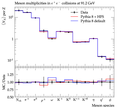
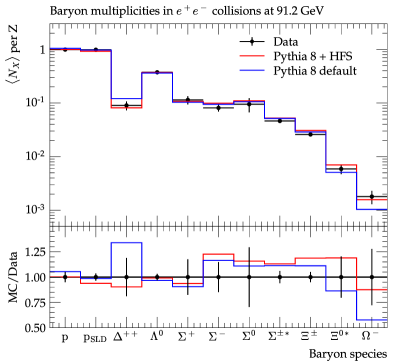
Figure 3: Yields of identified particles (per $\mathrm{Z}$) in $\mathrm{e}^{+}\mathrm{e}^{-}$ collisions at the $\mathrm{Z}$ pole. Mesons to the left, and baryons to the right. The P YTHIA default tune (in blue) is compared with the model extension with reasonable parameters (in red), as described in the text. Data are from various LEP experiments and SLD, with references in the text.

In figure 3 we show hadron yields per $\mathrm{Z}$ boson from $\mathrm{e}^{+}\mathrm{e}^{-}$ collisions at the $\mathrm{Z}$ pole. The model addition based on HFS is shown in red, and compared to default P YTHIA in blue. There are many parameter combinations which can describe $\mathrm{e}^{+}\mathrm{e}^{-}$ yields at a reasonable level, not least because the experimental error bars on the rare mesons and baryons, which are most sensitive to the presented model additions, are rather large. Hence, it also makes little sense to perform the tuning as a global $\chi^{2}$ minimization or similar. The strategy used is as follows, resulting parameters are listed in table 1:

• Event shape observables will not change, as the parton shower is left untouched, and Lund fragmentation function parameters $a$ and $b$ are fixed to default values. Also the total charged or $\pi^{\pm}$ multiplicity is left almost unchanged.

• A value of the parameter $\rho$ is chosen, such that kaons from the pseudoscalar nonet is reproduced at least as well as in the default tune.

• A value of the parameter $\xi$ is chosen, such that our updated proton multiplicity is well reproduced. In figure 3 (right) we show the proton multiplicity from SLD next to it for comparison.

• Values for parameters $y_{\mathrm{m1}}$ and $y_{\mathrm{m2}}$ are chosen such that all recorded mesons in the vector nonet are now reproduced within error bars.

• Parameters for $\eta$ and $\eta^{\prime}$ suppression are chosen to reproduce the yields form the default tune.

• Parameters $y_{\mathrm{diq}}$ and $c$ are chosen to give a reasonable description of $\Delta^{++}$ and $\Omega^{-}$.

Parameter name	P YTHIA name	Default value	Retuned value
$\rho$	StringFlav:probStoUD	0.21	0.19
$\xi$	StringFlav:probQQtoQ	0.81	0.072
$y_{\mathrm{diq}}$	StringFlav:probQQ1toQQ0	0.0275	0.04
$x$	StringFlav:probSQtoQQ	0.915	1 (fixed)
-	StringFlav:etaSup	0.60	0.55
-	StringFlav:etaPrimeSup	0.12	0.11
-	StringFlav:mesonUDvector	0.50	-
-	StringFlav:mesonSvector	0.55	-
$c$	-	-	0.65
$y_{\mathrm{m1}}$	-	-	0.4
$y_{\mathrm{m2}}$	-	-	0.25

Table 1: Table of parameters for the default (Monash 2013 [13]) and updated fragmentation model, listed with parameter names as given in this manuscript in the first column, P YTHIA names (when applicable) in the second column, followed by the default and retuned values. As it can be seen directly from the table, the number of free parameters in the default and the updated models are the same.

5 Results for ep and pp

In this section we go on to study $\mathrm{ep}$ and pp collisions, using the updated fragmentation model with parameters listed in table 1. We first note that while some effects are expected, the default P YTHIA description already does a reasonable job for most relevant observables, so enormous effects are not expected. This is also not the point. As indicated in the introduction, the main goal of this paper is to establish a more thorough baseline for further studies.

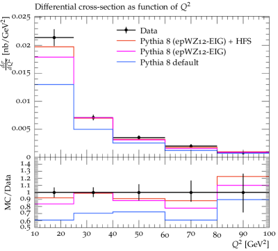
Figure 4: To the left we show $\phi$ production as function of $Q^{2}$ in neutral current DIS, as measured by ZEUS [45], compared to P YTHIA default (blue), P YTHIA with the epWZ12-EIG PDF (magenta) and finally with the hyperfine splitting effect (HFS) added on top (red). To the right we show hadron yields measured by ALICE in low multiplicity pp collisions at 7 TeV ($\pi^{\pm}$, $\mathrm{K^{0}_{s}}$, $\mathrm{p}$, $\Lambda^{0}$, $\Xi^{\pm}$ and $\Omega^{-}$) [1] and 13 TeV ($\mathrm{K}^{*0}$ and $\phi$) [46]. The data is again compared to P YTHIA default (blue) and with the HFS effects added (red).

In $\mathrm{ep}$ collisions, results from ZEUS [45] from 2002 on inclusive $\phi$ production in neutral current DIS, showed a large enhancement with respect to expectation. The most stunning result from that paper is arguably the $\phi$ cross section in the target region at small Bjorken $x$ (less than $\approx 0.006$), which is more than a factor of 2 above expectation. Indeed this result was taken as a clear indication of an enhanced strange sea in the proton at small $x$. As the P YTHIA DIS description is generally not capable of correctly describing basic particle multiplicities at small $x$ in the target region, we have to compare to some of the less spectacular results of the paper, still showing the same trend. In figure 4 (left) we show a comparison to the integrated (over $2\cdot 10^{-4}<x<10^{-2}$) $\phi$ cross section as function of $Q^{2}$. In blue we show P YTHIA default, which performs similarly as the HERWIG 5.1 Monte Carlo event generator [47] did in the original paper. Somewhat better agreement was achieved by the LEPTO 6.5 [48] and ARIADNE 4 [49] models, but only after an artificial decrease of the model parameters corresponding to the P YTHIA parameter $\rho$ (see section 2.1.2). Accounting for hyperfine splitting alone cannot bring P YTHIA in agreement with this data. In magenta we show the effect of changing the parton distribution function (PDF, through LHAPDF6 [50]) to one obtained by the ATLAS collaboration [51], where sensitivity to the strange quark density of protons on $\mathrm{W}^{\pm}$ and $\mathrm{Z}$ production at small $x$ is exploited. On top of this effect, we show (in red) the effect of hyperfine splitting, which makes the calculation compatible with data.

Going to pp collisions in figure 4 (right), we show comparisons to ALICE data at low forward multiplicity, at $\sqrt{s}=7$ TeV [1] and 13 TeV [46] respectively. At higher multiplicity we would expect rope effects (see section 1) to dominate, in particular for multi-strange baryon production, which is why we limit ourselves to the lowest multiplicity class. Even the lowest multiplicity class is, however, not completely free from overlapping strings, but as close as one can get in a $\mathrm{pp}$ collision. We note that there is about a factor of six between the $\mathrm{e}^{+}\mathrm{e}^{-}$ results in figure 3 and the pp results in figure 4 (right). Accounting for the different rapidity ranges, a factor of two remains. In the string model, this gives the direct interpretation that these events corresponds to two strings, meaning exchange of a single gluon or Pomeron. The exception to this argument is $\Omega^{-}$ production, on which we comment separately below.

All hadron multiplicities are described to the same level or better than P YTHIA default. There are two interesting points to be mentioned, pointing towards future work. First of all, we see that even with retuning to the lower proton yield in $\mathrm{e}^{+}\mathrm{e}^{-}$, P YTHIA still overshoots the proton multiplicity in low multiplicity pp collisions, giving apparent tension between the description of pp and $\mathrm{e}^{+}\mathrm{e}^{-}$. This leaves two possibilities. Either one of the data sets cannot be trusted – we re-iterate that the $\mathrm{e}^{+}\mathrm{e}^{-}$ results also had notable internal tension – or a key physics ingredient is missing. In the first case, future studies could consider simply leaving the proton yields out of the $\mathrm{e}^{+}\mathrm{e}^{-}$ tuning efforts, and instead tune to low multiplicity pp. Secondly, the $\Omega^{-}$ yield is still not well described, even with the baseline changed. This marks an opportunity for future studies of the rope model. We re-iterarate the argument above, that the low-multiplicity collisions should correspond roughly to two strings, leaving room for string overlap. We remark that also previous literature [1] showed an effect of rope formation for $\Omega^{-}$ production, even in the lowest multiplicity bin. Our result confirms that even with further attention given to the $\mathrm{e}^{+}\mathrm{e}^{-}$ baseline, there is still room for collective effects in low multiplicity pp. This is potentially a game-changing realization, as it is common for experimental analyses of small system collectivity, to use low multiplicity collisions as a no-collectivity baseline. This result suggests that the common strategy might be flawed. We will follow this point up in a future paper.

6 Conclusion

The Lund string model and its basic recipe for string breakings and formation of hadrons from the ingoing quarks and anti-quarks, has been a cornerstone of the P YTHIA Monte Carlo event generator, and provided the basis for many phenomenological and experimental studies in $\mathrm{e}^{+}\mathrm{e}^{-}$, $\mathrm{ep}$, and pp, mostly in an unchanged form since it’s first versions in the 1980s. In this paper we have updated the model to account for the impact of light quark mass differences, giving rise to modifications in the hadronic wave functions. With a simple ansatz, and no further parameters added to the model, we manage to improve in particular the description of $\rho^{\pm}$, $\omega$, $\Delta^{++}$ and $\Omega^{-}$ yields in $\mathrm{e}^{+}\mathrm{e}^{-}$ collisions. With this update, as well as by using updated PDFs, it is also possible to give a reasonable description of integrated $\phi$ production in neutral current DIS, and the updated baseline makes future precision studies of strangeness enhancement in pp using the rope hadronization model possible.

References

- [1] ALICE Collaboration, J. Adam et. al., “Enhanced production of multi-strange hadrons in high-multiplicity proton-proton collisions,” Nature Phys. 13 (2017) 535–539, 1606.07424.
- [2] J. Rafelski and B. Müller, “Strangeness Production in the Quark - Gluon Plasma,” Phys. Rev. Lett. 48 (1982) 1066. [Erratum: Phys.Rev.Lett. 56, 2334 (1986)].
- [3] P. Koch, J. Rafelski, and W. Greiner, “Strange hadron in hot nuclear matter,” Phys. Lett. B 123 (1983) 151–154.
- [4] P. Koch, B. Müller, and J. Rafelski, “Strangeness in Relativistic Heavy Ion Collisions,” Phys. Rept. 142 (1986) 167–262.
- [5] B. Andersson, G. Gustafson, G. Ingelman, and T. Sjöstrand, “Parton Fragmentation and String Dynamics,” Phys. Rept. 97 (1983) 31–145.
- [6] B. R. Webber, “A QCD Model for Jet Fragmentation Including Soft Gluon Interference,” Nucl. Phys. B 238 (1984) 492–528.
- [7] S. Gieseke, P. Kirchgaeßer, and S. Plätzer, “Baryon production from cluster hadronisation,” Eur. Phys. J. C 78 (2018), no. 2 99, 1710.10906.
- [8] C. B. Duncan and P. Kirchgaeßer, “Kinematic strangeness production in cluster hadronization,” Eur. Phys. J. C 79 (2019), no. 1 61, 1811.10336.
- [9] C. Bierlich, G. Gustafson, L. Lönnblad, and A. Tarasov, “Effects of Overlapping Strings in pp Collisions,” JHEP 03 (2015) 148, 1412.6259.
- [10] C. Bierlich and J. R. Christiansen, “Effects of color reconnection on hadron flavor observables,” Phys. Rev. D 92 (2015), no. 9 094010, 1507.02091.
- [11] J. R. Christiansen and P. Z. Skands, “String Formation Beyond Leading Colour,” JHEP 08 (2015) 003, 1505.01681.
- [12] ALICE Collaboration, S. Acharya et. al., “ Production and Baryon-to-Meson Ratios in pp and p-Pb Collisions at =5.02 TeV at the LHC,” Phys. Rev. Lett. 127 (2021), no. 20 202301, 2011.06078.
- [13] P. Skands, S. Carrazza, and J. Rojo, “Tuning PYTHIA 8.1: the Monash 2013 Tune,” Eur. Phys. J. C 74 (2014), no. 8 3024, 1404.5630.
- [14] T. Sjöstrand, S. Ask, J. R. Christiansen, R. Corke, N. Desai, P. Ilten, S. Mrenna, S. Prestel, C. O. Rasmussen, and P. Z. Skands, “An introduction to PYTHIA 8.2,” Comput. Phys. Commun. 191 (2015) 159–177, 1410.3012.
- [15] T. Sjöstrand, “The Lund Monte Carlo for Jet Fragmentation and Physics: JETSET Version 6.2,” Comput. Phys. Commun. 39 (1986) 347–407.
- [16] E. Brezin and C. Itzykson, “Pair production in vacuum by an alternating field,” Phys. Rev. D 2 (1970) 1191–1199.
- [17] B. Andersson, G. Gustafson, and J. Samuelsson, “Correlations in the hadronization process,” Z. Phys. C 64 (1994) 653–658.
- [18] X. Artru, “Classical String Phenomenology. 1. How Strings Work,” Phys. Rept. 97 (1983) 147.
- [19] J. S. Schwinger, “On gauge invariance and vacuum polarization,” Phys. Rev. 82 (1951) 664–679.
- [20] T. Sjöstrand, “Jet Fragmentation of Nearby Partons,” Nucl. Phys. B 248 (1984) 469–502.
- [21] B. Andersson, G. Gustafson, and B. Söderberg, “A General Model for Jet Fragmentation,” Z. Phys. C 20 (1983) 317.
- [22] I. Cohen et. al., “Electroproduction of Mesons,” Phys. Rev. D 25 (1982) 634.
- [23] B. Andersson, G. Gustafson, and T. Sjöstrand, “A Model for Baryon Production in Quark and Gluon Jets,” Nucl. Phys. B 197 (1982) 45–54.
- [24] B. Andersson, G. Gustafson, and T. Sjöstrand, “Baryon Production in Jet Fragmentation and Decay,” Phys. Scripta 32 (1985) 574.
- [25] A. Casher, H. Neuberger, and S. Nussinov, “Chromoelectric Flux Tube Model of Particle Production,” Phys. Rev. D 20 (1979) 179–188.
- [26] C. Bierlich et. al., “Robust Independent Validation of Experiment and Theory: Rivet version 3,” SciPost Phys. 8 (2020) 026, 1912.05451.
- [27] M. Krishnamoorthy, H. Schulz, X. Ju, W. Wang, S. Leyffer, Z. Marshall, S. Mrenna, J. Müller, and J. B. Kowalkowski, “Apprentice for Event Generator Tuning,” EPJ Web Conf. 251 (2021) 03060, 2103.05748.
- [28] Particle Data Group Collaboration, P. A. Zyla et. al., “Review of Particle Physics,” PTEP 2020 (2020), no. 8 083C01.
- [29] ALEPH Collaboration, R. Barate et. al., “Studies of quantum chromodynamics with the ALEPH detector,” Phys. Rept. 294 (1998) 1–165.
- [30] G. S. Abrams et. al., “Measurements of Charged Particle Inclusive Distributions in Hadronic Decays of the Boson,” Phys. Rev. Lett. 64 (1990) 1334.
- [31] OPAL Collaboration, K. Ackerstaff et. al., “Measurements of flavor dependent fragmentation functions in events,” Eur. Phys. J. C 7 (1999) 369–381, hep-ex/9807004.
- [32] DELPHI Collaboration, P. Abreu et. al., “ and production in , , ,” Eur. Phys. J. C 5 (1998) 585–620.
- [33] DELPHI Collaboration, P. Abreu et. al., “Production characteristics of and light meson resonances in hadronic decays of the ,” Z. Phys. C 65 (1995) 587–602.
- [34] DELPHI Collaboration, P. Abreu et. al., “Measurement of inclusive (892), (1020) and (1430) production in hadronic decays,” Z. Phys. C 73 (1996) 61–72.
- [35] ALEPH Collaboration, D. Buskulic et. al., “Inclusive production of neutral vector mesons in hadronic decays,” Z. Phys. C 69 (1996) 379–392.
- [36] OPAL Collaboration, P. D. Acton et. al., “A Measurement of (892) production in hadronic decays,” Phys. Lett. B 305 (1993) 407–414.
- [37] OPAL Collaboration, K. Ackerstaff et. al., “Spin alignment of leading (892) mesons in hadronic decays,” Phys. Lett. B 412 (1997) 210–224, hep-ex/9708022.
- [38] OPAL Collaboration, K. Ackerstaff et. al., “Production of (980), (1270) and (1020) in hadronic decay,” Eur. Phys. J. C 4 (1998) 19–28, hep-ex/9802013.
- [39] SLD Collaboration, K. Abe et. al., “Production of , , , , , and in hadronic decays,” Phys. Rev. D 59 (1999) 052001, hep-ex/9805029.
- [40] SLD Collaboration, K. Abe et. al., “Production of , , , , p and in Light (), and Jets from Decays,” Phys. Rev. D 69 (2004) 072003, hep-ex/0310017.
- [41] ALEPH Collaboration, R. Barate et. al., “A Measurement of the semileptonic branching ratio BR(-baryon ) and a study of inclusive , , production in decays,” Eur. Phys. J. C 5 (1998) 205–227.
- [42] OPAL Collaboration, R. Akers et. al., “Measurement of the production rates of charged hadrons in annihilation at the ,” Z. Phys. C 63 (1994) 181–196.
- [43] DELPHI Collaboration, P. Abreu et. al., “Inclusive measurements of the and production in hadronic decays,” Nucl. Phys. B 444 (1995) 3–26.
- [44] OPAL Collaboration, G. Alexander et. al., “Strange baryon production in hadronic decays,” Z. Phys. C 73 (1997) 569–586.
- [45] ZEUS Collaboration, S. Chekanov et. al., “Observation of the strange sea in the proton via inclusive phi meson production in neutral current deep inelastic scattering at HERA,” Phys. Lett. B 553 (2003) 141–158, hep-ex/0211025.
- [46] ALICE Collaboration, S. Acharya et. al., “Multiplicity dependence of (892) and (1020) production in pp collisions at =13 TeV,” Phys. Lett. B 807 (2020) 135501, 1910.14397.
- [47] G. Marchesini, B. R. Webber, G. Abbiendi, I. G. Knowles, M. H. Seymour, and L. Stanco, “HERWIG: A Monte Carlo event generator for simulating hadron emission reactions with interfering gluons. Version 5.1 - April 1991,” Comput. Phys. Commun. 67 (1992) 465–508.
- [48] G. Ingelman, A. Edin, and J. Rathsman, “LEPTO 6.5: A Monte Carlo generator for deep inelastic lepton-nucleon scattering,” Comput. Phys. Commun. 101 (1997) 108–134, hep-ph/9605286.
- [49] L. Lönnblad, “ARIADNE version 4: A Program for simulation of QCD cascades implementing the color dipole model,” Comput. Phys. Commun. 71 (1992) 15–31.
- [50] A. Buckley, J. Ferrando, S. Lloyd, K. Nordström, B. Page, M. Rüfenacht, M. Schönherr, and G. Watt, “LHAPDF6: parton density access in the LHC precision era,” Eur. Phys. J. C 75 (2015) 132, 1412.7420.
- [51] ATLAS Collaboration, G. Aad et. al., “Determination of the strange quark density of the proton from ATLAS measurements of the and cross sections,” Phys. Rev. Lett. 109 (2012) 012001, 1203.4051.