Coded Distributed Computing with Pre-set Assignments of Data and Output Functions

Abstract

Coded distributed computing (CDC) can reduce the communication load for distributed computing systems by introducing redundant computation and creating multicasting opportunities. The optimal computation-communication tradeoff has been well studied for homogeneous systems, and some results have been obtained under heterogeneous conditions. However, the existing schemes require delicate data placement and output function assignment, which is not feasible in some practical scenarios when distributed nodes fetch data without the orchestration of a central server. In this paper, we consider the general heterogeneous distributed computing systems where the data placement and output function assignment are arbitrary but pre-set (i.e., cannot be designed by schemes). For this general heterogeneous setup, we propose two coded computing schemes, One-Shot Coded Transmission (OSCT) and Few-Shot Coded Transmission (FSCT), to reduce the communication load. These two schemes first group the nodes into clusters and divide the transmission of each cluster into multiple rounds, and then design coded transmission in each round to maximize the multicast gain. The key difference between OSCT and FSCT is that the former uses a one-shot transmission where each encoded message can be decoded independently by the intended nodes, while the latter allows each node to jointly decode multiple received symbols to achieve potentially larger multicast gains. Furthermore, with theoretical converse proofs, we derive sufficient conditions for the optimality of OSCT and FSCT, respectively. This not only recovers the existing optimality results known for homogeneous systems and 3-node systems, but also includes some cases where our schemes are optimal while other existing methods are not.

I Introduction

Distributed computing such as MapReduce [1] and Spark [2] has been widely applied in practice, as it can exploit distributed storage and computing resources to improve the reliability and reduce the computation latency. In the MapReduce-type framework, the computation task is decomposed into three phases: Map phase, Shuffle phase, and Reduce phase. In the Map phase, a master server splits the input files into multiple subfiles and assigns the subfiles to distributed computing nodes to generate intermediate values (IVs). Then, the IVs are exchanged among the distributed computing nodes during the Shuffle phase. In the Reduce phase, the computing nodes use the obtained IVs to compute the reduce the output functions. For large-scale computation tasks, the Map phase may generate a massive numbers of IVs, which in turn causes the communication bottleneck in the Shuffle phase, i.e., the communication latency could occupy a large proportion of the total execution time. For instance, it is observed that 70% of the overall job execution time is spent during the Shuffle phase when running a self-Join[3] application on an Amazon EC2 cluster[4].

Recently, many coded computing techniques have been proposed to mitigate the communication bottleneck for distributed computing systems. In particular, Li et al. proposed a coded distributed computing (CDC) scheme for MapReduce-type systems to reduce the communication load [5]. The key idea of CDC is to introduce redundant computation in the Map phase and create multicast opportunities in the Shuffle phase. A theoretical tradeoff between computation load and communication load was also established in [5] which shows that increasing the computation load in the Map phase by a factor $r$ (representing the total number of computed files by all nodes normalized by the total number of files) can reduce the communication load in the Shuffle phase by the same factor $r$. Due to its promising performance and theoretical optimality, the CDC technique has attracted wide interest and has been applied in many applications such as Artificial Intelligence (AI), the Internet of Things, and edge computing (see a survey paper in [6]). For instance, the performance of CDC was evaluated on the TeraSort[7] on Amazon EC2 clusters[4], which can achieve a $1.97\times-3.39\times$ speedup compared with the uncoded scheme for typical settings of interest[5]. In [8] the CDC-based approach has been applied to distributed multi-task learning (MTL) systems, and experiments on the MNIST dataset show that the total execution time is reduced by about 45% compared to the traditional uncoded method when computation load $r=3$ and the number of tasks $m=4$. In [9] it proposed a flexible and low-complexity design for the CDC scheme.

The CDC technique for various homogenous systems with equal computing or storage capabilities has been extensively investigated. For instance, the authors in [10] established an alternative tradeoff between computation load and communication load under a predefined storage constraint. Also, different approaches have been proposed to further reduce the communication cost of CDC. Works in [11, 12, 13, 14, 15, 16, 17] focused on the data placement of the system or the construction of the coded messages, and [18, 19, 20] applied compression and randomization techniques to design the coded shuffling strategy. In particular, the authors in [12] presented an appropriate resolvable design based on linear error correcting codes to avoid splitting the input file into too tiny pieces, and this resolvable design based scheme was used in [14] to solve the limitation of the compressed CDC scheme[18]. By applying the concept of the placement delivery array (PDA) to the distributed computation framework, [15, 16, 17] further reduced the number of subfiles and the number of output functions. By combining the compression with coding techniques, several IVs of a single computation task can be compressed into a single pre-combined value[18], and the same idea can also be extended to distributed machine learning, such as Quantized SGD[19], which is a compression technique used to reduce communication bandwidth during the gradient updates between the computing nodes.

Note that in practical distributing systems the computing nodes could have different storage and computational capabilities. To address the heterogeneous problem, several works have considered the heterogeneous distributed computing (HetDC) system and proposed coded computing schemes to reduce the communication load [21, 22, 23, 24]. In [21], the authors characterized the information-theoretically minimum communication load for the 3-node system with arbitrary storage size at each node. In [22], the authors proposed a combinatorial design that operates on non-cascaded heterogeneous networks where nodes have varying storage and computing capabilities but each Reduce function is computed exactly once. A cascaded HetDC system was considered in [23], where each Reduce function is allowed to be computed at multiple nodes. The communication load obtained in [23] is optimal within a constant factor given their proposed mapping strategies. The authors in [24] characterized the upper bound of the optimal communication load as a linear programming problem, and jointly designed the data placement, Reduce function allocation and data shuffling strategy to reduce the communication load. However, all existing schemes [21, 22, 23, 24] require delicate data placement and output function assignment (i.e., the data stored by each node and the set of output functions computed by each node both are design parameters), which is not feasible in some practical scenarios when the nodes fetch data without the orchestration of a central server, or when each node autonomously determines its desired output functions. For instance, in [25, 26] each user randomly and independently fetches a subset of all data from a central server, and in distributed multi-task learning [27, 8] the users wish to learn their own model depending on its task goal. Until now, there exists no work considering the HetDC systems with pre-set data placement and output function assignment, i.e., the data placement and output function assignment are system parameters that cannot be designed by schemes.

I-A Main Contributions

In this paper, we consider the general HetDC system with arbitrary but pre-set data placement and Reduce function assignment (general HetDC system in short). We aim to find coded distributed computing schemes that are applicable to arbitrary HetDC system and characterize the theoretical computation-communication tradeoff. The main contributions of this paper are summarized as follows:

• To the best of our knowledge, our work is the first attempt to study the general HetDC system with arbitrary and pre-set data placement and Reduce function assignment. This is a challenging problem because when the data placement at nodes is asymmetric and different Reduce functions are computed by different numbers of nodes, the IVs to be shuffled can be distributed in an extremely irregular manner, prohibiting designing the data shuffling strategy with the help of input files and Reduce functions allocations. This makes all previous schemes in [21, 22, 23, 24] infeasible for the general HetDC system (see detailed discussions in Section III-C). To address this challenge, we first characterize the heterogeneities of the HetDC system from the perspective of computing nodes, input files, and IVs, respectively, and then design data shuffling schemes based on these heterogeneities.

• We propose two CDC approaches for the general HetDC system, namely One-Shot Coded Transmission (OSCT) and Few-Shot Coded Transmission (FSCT). By grouping nodes into clusters with different sizes and carefully categorizing IVs, OSCT delicately designs the size of the encoded messages by solving an optimization problem that maximizes the multicast opportunities, and sends each message block in a one-shot manner where each message block can be decoded independently by the intended nodes. To further exploit the gain of multicasting, FSCT splits IVs into smaller pieces and sends each message block in a few-shot manner where each node needs to jointly decode multiple received message blocks to obtain its desired IVs. Numerical results show that both OSCT and FSCT achieve lower communication loads than those of the state-of-the-art schemes, and FSCT can potentially improve OSCT at the cost of higher coding complexity.

• We establish optimality results on the fundamental computation-communication tradeoff for some types of general HetDC systems, and derive the sufficient conditions for the optimality of OSCT and FSCT, respectively. In particular, we associate the optimality of OSCT with an optimization problem and prove that OSCT is optimal if the optimal value of the objective function is zero. For the FSCT scheme, we first introduce the concept of deficit ratio for each computing node, which is the ratio between the number of IVs that the node desires and the number of IVs that the node locally knows. Then we present two conditions: deficit condition and feasible condition, and prove that if these two conditions are satisfied for all nodes in each cluster, the system is well-balanced and FSCT is optimal. This not only recovers the existing optimality results known for homogeneous systems [5] and 3-node systems [21], but also includes some cases where our schemes are optimal while other existing methods are not.

I-B Comparison with Coded Caching Schemes

The CDC-based approaches are closely related to coded caching scheme that was first proposed by Maddah-Ali and Niesen [28], as they both involve repetitive data placement and coded multicasting. Our coded computing schemes can also be applied to the heterogeneous coded caching setup where each user has an arbitrary but pre-set data placement and requires an arbitrary set of files. To the best of our knowledge, there exists no coded caching scheme proposed for this setup. In the following, we compare the related works in coded caching under heterogeneous setups with our schemes from the perspective of problem formulation and algorithm design.

The coded caching problem with non-uniform file popularity was considered in [29, 30, 31, 32]. In this setup, one server has a library of $N$ files and each user independently requests file $n\in[N]$ with probability $p_{n}$. Authors in [29] proposed a file gouping method where the files were partitioned into groups with uniform popularities to preserve the symmetry within each group. Following the idea of file grouping, a specific multi-level file popularity model was considered in [30] and an order-optimal scheme was derived. The work in [31] considered a more general system with arbitrary popularity distribution. The scheme divided the files into 3 groups using a simple threshold and attained a constant-factor performance gap under all popularity distributions. An optimization approach was proposed in [32], where each file was partitioned into $2^{K}$ non-overlapping subfiles and the placement strategy was optimized to minimize the average load. This scheme focused on the design of file partitions, while ours focus on the design of coded messages. Note that among all literature mentioned above, each node requires only one file at a time and their cache sizes were uniform, while in our work the data placement and the number of functions computed by each node both are arbitrary and could be non-uniform.

The coded caching problem with the heterogeneity of user demand has been studied in [33, 34, 35]. In their setups, users have distinct distributions of demands, and the set of files that different users may desire can possibly overlap. However, they assumed that each user requests only one file at a time. There are also some works considering the case when users demand multiple files at each time[36][37]. Specifically, authors in [36] developed a new technique for characterizing information-theoretic lower bounds in both centralized content delivery and device-to-device distributed delivery. In [37], an order-optimal scheme based on the random vector (packetized) caching placement and multiple group cast index coding was proposed. However, the works above considered the homogeneous case where each user has a cache of size $M$ files and requests $L\geq 1$ files independently according to a common demand distribution, while we allow arbitrary storage and computation capabilities for each node.

For the coded caching setup with distinct file size, [38] categorized all files into $T$ types by their size, and each user $k$ will cache $q_{\ell}F_{\ell}$ bits of every file in $\ell$-th type. By carefully deciding the caching parameter $q_{l}$ based on the number of files with the same type, the proposed scheme achieved optimal load within a constant gap to the proposed lower bound. For the setup with distinct cache sizes, [39] considered a centralized system in which cache sizes of different users were not necessarily equal. The authors proposed an achievable scheme optimized by solving a linear program, where each file was split into $2^{K}$ subfiles and the sizes of partitions were determined by an optimization problem. In [40], the authors considered a more general setting with arbitrary file and cache size. By first proposing a parameter-based decentralized coded caching scheme and then optimizing the caching parameter, this work provided an optimization-based solution and an iterative algorithm. All aforementioned works considered heterogeneous file sizes or storage capabilities, but the data placement is still free to design, differing from our setting that has arbitrary and present data placement. Meanwhile, the demand for each node is homogeneous, where the request for each node is a single file, while in our setting each node could have multiple requests (Reduce functions), and the demand for every node is arbitrary.

Some works have considered multiple types of non-uniform parameters, such as[41, 42]. In [41], the authors studied fully heterogeneous cases under distinct file sizes, unequal cache size, and user-dependent heterogeneous file popularity. They characterized the exact capacity for a two-file two-user system, while we focus on the coding strategy design in the general case with an arbitrary number of users. In [42], an optimization framework to design caching schemes with distinct file sizes, unequal cache size, and non-uniform file popularity was proposed. This framework is based on exquisitely designing data placement, which differs from our assumption of pre-set data and output function assignment.

The rest of this paper is organized as follows. Section II introduces our problem formulation, including the system model and useful definitions. Section III presents the main results of this paper. Section IV gives some examples of our two achievable schemes: OSCT and FSCT. Sections V and VI present OSCT and FSCT, respectively. Section VII concludes this paper.

Notations: Let $[n]$ denote the set $\{1,2,\cdots,n\}$ for some $n\in\mathbb{Z}^{+}$, where $\mathbb{Z}^{+}$ is the set of positive integers. $\mathbb{Q}^{+}$ denotes the set of positive rational numbers. For a set $\mathcal{S}$, let $|\mathcal{S}|$ denote its cardinality. For a vector $\boldsymbol{v}$, let $\boldsymbol{v}[i]$ denote its $i_{th}$ element. $(x)^{+}$ denotes the positive part of $x$, i.e., $(x)^{+}=x$ for $x\geq 0$ and $(x)^{+}=0$ for $x<0$. Given an event $\mathscr{E}$, we use $\mathds{1}(\mathscr{E})$ as an indicator, i.e., equals to 1 if the event happens, and 0 otherwise.

II Problem Formulation

Consider a MapReduce-type system that aims to compute $Q$ output functions from $N$ input files with $K$ distributed nodes, for some positive integers $K,Q,N$. The $N$ input files are denoted by ${w_{1},\dots,w_{N}}\in\mathbb{F}_{2^{F}}$, and the $Q$ output functions are denoted by $\phi_{1},\dots,\phi_{Q}$, where $\phi_{q}$: $(\mathbb{F}_{2^{F}})^{N}\rightarrow\mathbb{F}_{2^{B}}$, $q\in[Q]$, maps all input files into a ${B}$-bit output value $u_{q}=\phi_{q}(w_{1},\dots,w_{N})\in\mathbb{F}_{2^{B}}$, for some ${B}\in\mathbb{Z}^{+}$.

Node $k$, for $k\in[K]$, is required to map a subset of input files and compute a subset of output functions. Denote the indices of input files mapped by Node $k$ as $\mathcal{M}_{k}\subseteq[N]$ and the indices of output functions computed by $k$ as $\mathcal{W}_{k}\subseteq[Q]$. To ensure that all input files are stored and all Reduce functions are computed, we have $\bigcup_{k\in[K]}\mathcal{M}_{k}=[N]$ and $\bigcup_{k\in[K]}\mathcal{W}_{k}=[Q]$.

Unlike the existing CDC-based works (e.g., [5, 23, 24]) in which the data placement $\mathcal{M}=\{\mathcal{M}_{k}\}_{k=1}^{K}$ and Reduce functions assignment $\mathcal{W}=\{\mathcal{W}_{k}\}_{k=1}^{K}$ are to be designed by schemes, here we consider the general HetDC system where

• $\{\mathcal{M}_{k}\}_{k=1}^{K}$ and $\{\mathcal{W}_{k}\}_{k=1}^{K}$ are pre-set.

• $\{|\mathcal{M}_{k}|\}_{k=1}^{K}$ and $\{|\mathcal{W}_{k}|\}_{k=1}^{K}$ are arbitrary and unnecessarily equal, i.e., it is possible to have $|\mathcal{M}_{i}|\neq|\mathcal{M}_{j}|,|\mathcal{W}_{i}|\neq|\mathcal{W}_{j}|$, for some $i,j\in[K],i\neq j$.

In the MapReduce framework, there are $N$ Map functions $\vec{g}_{n}=(g_{1,n},\dots,g_{Q,n}):\,\mathbb{F}_{2^{F}}\rightarrow(\mathbb{F}_{2^{V}})^{Q},$ for each file $n\in[N]$, and each $g_{q,n}$ maps the corresponding file into $Q$ intermediate values (IVs) $v_{q,n}=g_{q,n}(w_{n})\in\mathbb{F}_{2^{V}}$. Here $V$ denotes the bit-length of a single IV. Meanwhile, for each output function $\phi_{q}$, there is a corresponding Reduce function $h_{q}(v_{q,1},\dots,v_{q,N}):(\mathbb{F}_{2^{V}})^{N}\rightarrow\mathbb{F}_{2^{B}}$, which maps the corresponding IVs from all input files into the output value $u_{q}$, for $q\in[Q]$. Combining the Map and Reduce functions, we have $u_{q}=\phi_{q}(w_{1},\!\ldots\!,w_{N}\!)\!=\!h_{q}\!\left(g_{q,1}(w_{1}),\!\ldots\!,g_{q,{N}}(w_{N})\right).$

The system consists of three phases: Map, Shuffle and Reduce.

II-1 Map Phase

Node $k$, for $k\in[K]$, uses the Map functions to map its stored input files, and obtains local IVs $\{v_{q,n}:q\in[Q],n\in\mathcal{M}_{k}\}$.

II-2 Shuffle Phase

Based on the local mapped IVs, Node $k$, for $k\in[K]$, generates an $\ell_{k}$-bit message $X_{k}$ using some encoding functions $e_{k}:\left(\mathbb{F}_{2^{V}}\right)^{Q|\mathcal{M}_{k}|}\rightarrow\mathbb{F}_{2^{\ell_{k}}}$ such that

$$X_{k}=e_{k}(\{v_{q,n}:q\in[Q],n\in\mathcal{M}_{k}\}).$$ (1)

Then Node $k$ broadcasts $X_{k}$ to other nodes. After the Shuffle phase, each node receives messages $X_{1},X_{2},\cdots,X_{K}$.

II-3 Reduce Phase

In this phase, each node first recovers all required IVs and then computes the assigned Reduce functions. More specifically, Node $k$ recover its desired IVs based on the received message $X_{1},X_{2},\cdots,X_{K}$ and its local IVs using the decoding function $d_{k}:\mathbb{F}_{2^{\ell_{1}}}\times\mathbb{F}_{2^{\ell_{2}}}\times\cdots\times\mathbb{F}_{2^{\ell_{K}}}\times\left(\mathbb{F}_{2^{V}}\right)^{Q|\mathcal{M}_{k}|}\rightarrow\left(\mathbb{F}_{2^{V}}\right)^{N|\mathcal{W}_{k}|}$:

$$\{v_{q,n}:n\in[N],q\in\mathcal{W}_{k}\}=d_{k}\left(X_{1},X_{2},\cdots,X_{K},\{v_{q,n}:q\in[Q],n\in\mathcal{M}_{k}\}\right).$$

Then Node $k$ computes the assigned Reduce functions and get the output values $u_{q}=h_{q}(v_{q,1},\dots,v_{q,N})$, for $q\in\mathcal{W}_{k}$.

Definition 1 (Computation load and Communication load[5]).

The computation load is defined as the number of files mapped across the $K$ nodes normalized by the total number of files, i.e. $r\triangleq{\sum_{k\in[K]}|\mathcal{M}_{k}|}/{N}$. The communication load is defined as the total number of bits (normalized by $NQV$) communicated by the $K$ nodes in the Shuffle phase, i.e., $L\triangleq\frac{\sum\limits_{k\in[K]}\ell_{k}}{NQV}$.

We say that a communication load $L(\mathcal{M},\mathcal{W})$ is feasible under pre-set data placement $\mathcal{M}$ and Reduce function assignment $\mathcal{W}$, if for any $\epsilon>0$, we can find a set of encoding functions and decoding functions that achieve the communication load $\tilde{L}(\mathcal{M},\mathcal{W})$ s.t. $|L(\mathcal{M},\mathcal{W})-\tilde{L}(\mathcal{M},\mathcal{W})|\leq\epsilon$ and Node $k\in[K]$ can successfully compute all the desired output functions $\{u_{q}:q\in\mathcal{W}_{k}\}$.

Definition 2.

The optimal communication load $L^{*}$ is defined as

$$L^{*}(\mathcal{M},\mathcal{W})=\inf\{L(\mathcal{M},\mathcal{W}):L(\mathcal{M},\mathcal{W})\ \textnormal{is feasible}\}.$$

Given the pre-set data placement and Reduce function assignment, we present two homogeneous setups.

Definition 3 (Homogeneous System[5]).

A MapReduce system with pre-set data placement $\mathcal{M}$ and Reduce function assignment $\mathcal{W}$ is called homogeneous if it satisfies the following conditions: (1) the data placement is symmetric where $N$ input files are evenly partitioned into $\tbinom{K}{r}$ disjoint batches $\{\mathcal{B}_{\mathcal{T}}:\mathcal{T}\subset[K],|\mathcal{T}|=r\}$ for some $r\in[K]$, where each batch of files $\mathcal{B}_{\mathcal{T}}$ is mapped by Node $k$ if $k\in\mathcal{T}$, so every $r$ nodes will jointly map ${N}/{\tbinom{K}{r}}$ files; (2) $Q$ Reduce functions are evenly partitioned into $\tbinom{K}{s}$ disjoint batches $\{\mathcal{D}_{\mathcal{P}}:\mathcal{P}\subset[K],|\mathcal{P}|=s\}$ for some $s\in[K]$, where each batch of Reduce functions $\mathcal{D}_{\mathcal{P}}$ is computed by Node $k$ if $k\in\mathcal{P}$. Thus, every subset of $s$ node will jointly reduce ${Q}/{\tbinom{K}{s}}$ functions.

Definition 4 (Semi-Homogeneous System).

A MapReduce system with data placement $\mathcal{M}$ and Reduce function assignment $\mathcal{W}$ is called semi-homogeneous system if it satisfies the following conditions: (1) the data placement is the same as the homogeneous system in Definition 3; (2) the Reduce function assignment is multi-level symmetric, i.e., the $Q$ Reduce functions can be partitioned into $K$ disjoint sets: $\mathcal{Q}_{1},\cdots,\mathcal{Q}_{K}$ and each set of Reduce functions $\mathcal{Q}_{s}$ are evenly partitioned into $\tbinom{K}{s}$ disjoint batches $\{\mathcal{D}_{\mathcal{P}}:\mathcal{P}\subset[K],|\mathcal{P}|=s\}$ for some $s\in[K]$, where each batch of Reduce functions $\mathcal{D}_{\mathcal{P}}$ is computed by Node $k$ if $k\in\mathcal{P}$.

For the homogeneous system, the pre-set data placement and Reduce function assignment follow the symmetric design of cascaded distributed computing framework in [5], and each Reduce function will be computed by exactly $s$ nodes in a cyclic symmetric manner. In the semi-homogeneous system, we relax the constraint on Reduce function assignment such that the Reduce functions are divided into different sub-groups, and each Reduce function in the same group will be computed by exactly $s$ node in a cyclic symmetric manner. In particular, when only one sub-group exists, the semi-homogeneous system reduces to the homogeneous system.

Next, we introduce definitions to characterize the heterogeneities of the system from the perspective of computing nodes, input files, and IVs, respectively. From the perspective of computing nodes, we borrow the definitions of Mapping load and Reducing load from [24].

Definition 5 (Mapping load and Reducing load[24]).

The Mapping load for Node $k\in\mathcal{S}$ is defined as $m_{k}\triangleq\frac{|\mathcal{M}_{k}|}{N}\in[0,1]$, which denotes the fraction of files that Node $k$ mapped. Similarly, the Reducing load for Node $k$ is defined as $\omega_{k}\triangleq\frac{|\mathcal{W}_{k}|}{Q}\in[0,1]$.

From the perspective of input files, we introduce new definitions of Mapping times and Reducing times as follows:

Definition 6 (Mapping times and Reducing times).

The Mapping times of file $w_{i}$, denoted as $r_{i}$, for $i\in[N]$ is defined as the number of nodes who map file $w_{i}$. Then the minimum Mapping times of a system is defined as $r_{\textnormal{min}}\triangleq\min\limits_{1\leq i\leq N}r_{i}$. Similarly, the Reducing times of function $h_{i}$, denoted as $q_{i}$, for $i\in[Q]$ is defined as the number of nodes who compute Reduce function $h_{i}$. Then the minimum Reducing times of a system is defined as $q_{\textnormal{min}}\triangleq\min\limits_{1\leq i\leq Q}q_{i}$.

From the perspective of IVs, we first define $(z,\mathcal{S})$-mapped IVs and then define the deficit of Node $i\in\mathcal{S}$ as the ratio between the number of locally known IVs and the number of desired IVs at Node $i$. Before giving the formal definitions, we first define $\mathcal{V}^{\mathcal{S}\backslash\mathcal{S}_{1}}_{\mathcal{S}_{1}}$ as the set of IVs needed by all nodes in $\mathcal{S}\backslash\mathcal{S}_{1}$, no node outside $\mathcal{S}$, and known exclusively by nodes in $\mathcal{S}_{1}$, for some $\mathcal{S}\subseteq[K]$ and $\mathcal{S}_{1}\subset\mathcal{S}:|\mathcal{S}_{1}|\geq r_{\min}$, i.e.,

$$\mathcal{V}_{\mathcal{S}_{1}}^{\mathcal{S}\backslash\mathcal{S}_{1}} \triangleq \{v_{q,n}:q\in\underset{k\in\mathcal{S}\backslash\mathcal{S}_{1}}{\cap}{\mathcal{W}}_{k},q\notin\underset{k\notin\mathcal{S}}{\cup}{\mathcal{W}}_{k},n\in\underset{k\in{\mathcal{S}}_{1}}{\cap}\mathcal{M}_{k},n\notin\underset{k\notin\mathcal{S}_{1}}{\cup}{\mathcal{M}}_{k}\}.\qquad$$ (2)

Definition 7 ($(z,\mathcal{S})$-mapped IVs).

Given a subset $\mathcal{S}\subseteq[K]$ and an integer $r_{\min}\leq z\leq|\mathcal{S}|$, we define the $(z,\mathcal{S})$-mapped IVs, denoted by $\mathcal{V}_{z}^{\mathcal{S}}$, as the set of IVs required by $|\mathcal{S}|-z$ nodes and known exclusively by $z$ nodes in $\mathcal{S}$, i.e.,

$$\mathcal{V}_{z}^{\mathcal{S}}=\bigcup_{\mathcal{S}_{1}\subseteq\mathcal{S}:|\mathcal{S}_{1}|=z}\mathcal{V}_{\mathcal{S}_{1}}^{\mathcal{S}\backslash\mathcal{S}_{1}}.$$ (3)

Definition 8 (Deficit Ratio).

Given a system with data placement $\mathcal{M}$ and Reduce function assignment $\mathcal{W}$, we define the deficit ratio of Node $i$ on the $(z,\mathcal{S})$-mapped IVs $\mathcal{V}_{z}^{\mathcal{S}}$ as

$$\textit{D}(i,\mathcal{S},z)\triangleq\frac{\sum_{\begin{subarray}{c}S_{1}\subseteq\mathcal{S}:\\ |S_{1}|=z,i\not\in S_{1}\end{subarray}}|\mathcal{V}_{\mathcal{S}_{1}}^{\mathcal{S}\backslash\mathcal{S}_{1}}|}{\sum_{\begin{subarray}{c}S_{1}\subseteq\mathcal{S}:\\ |S_{1}|=z,i\in S_{1}\end{subarray}}|\mathcal{V}_{\mathcal{S}_{1}}^{\mathcal{S}\backslash\mathcal{S}_{1}}|}.$$ (4)

For convenience, we let $\textit{D}(i,\mathcal{S},z)=0$ when

$$\sum\limits_{\begin{subarray}{c}S_{1}\subseteq\mathcal{S}:|S_{1}|=z,i\not\in S_{1}\end{subarray}}|\mathcal{V}_{\mathcal{S}_{1}}^{\mathcal{S}\backslash\mathcal{S}_{1}}|=\sum\limits_{\begin{subarray}{c}S_{1}\subseteq\mathcal{S}:|S_{1}|=z,i\in S_{1}\end{subarray}}|\mathcal{V}_{\mathcal{S}_{1}}^{\mathcal{S}\backslash\mathcal{S}_{1}}|=0.$$

The deficit ratio $\textit{D}(i,\mathcal{S},z)$ characterizes the heterogeneity of a system at the IV level, which represents the ratio between the number of IVs required by Node $i$ and the number of files mapped by Node $i$ with respect to the $(z,\mathcal{S})$-mapped IVs. Since we consider the pre-set scenario where the data placement cannot be designed, the IVs could be distributed in an extremely irregular manner but previous definitions could not reveal this feature, which prompts us to introduce the above definition of deficit ratio.

III Main Results

In this section, we first present a lower bound of the optimal communication load proved in [43], and then we present two achievable upper bounds for the optimal communication load under pre-set data placement and Reduce function assignment. By comparing both upper and lower bounds, we show that our schemes are optimal in some non-trivial cases.

Lemma 1.

([43, Lemma 1]) Consider a distributed computing system with parameters $N$ and $Q$, given a data placement $\mathcal{M}$ and Reduce function assignment $\mathcal{W}$ that uses $K$ nodes. For any integers $t,d$, let $a_{t,d}$ denotes the number of intermediate values that are available at $t$ nodes, and required by (but not available at) $d$ nodes. The communication load of any valid shuffling design is lower bounded by:

$$L^{*}(\mathcal{M},\mathcal{W})\geq\frac{1}{QN}\sum_{t=1}^{K}\sum_{d=1}^{K-t}a_{t,d}\frac{d}{t+d-1}.$$ (5)

III-A One-shot Coded Transmission (OSCT)

III-A1 Upper bound of OSCT

Given a cluster $S\subseteq[K]$ and $z\in\mathbb{Z}$ with $r_{\min}\leq z\leq|\mathcal{S}|$, denote the $\binom{|\mathcal{S}|}{z}$ subsets of $S$ of size $z$ as $\mathcal{S}_{z}[1],\mathcal{S}_{z}[2],\cdots,\mathcal{S}_{z}[\binom{|\mathcal{S}|}{z}]$ respectively. The upper bound achieved by OSCT is given in the following theorem.

Theorem 1.

Consider the distributed computing system with $K$ nodes, $N$ files and $Q$ Reduce functions under pre-set data placement $\mathcal{M}$ and Reduce function assignment $\mathcal{W}$ for $k\in[K]$. The optimal communication load is upper bounded by $L^{*}\leq L_{\textnormal{OSCT}}$ where $L_{\textnormal{OSCT}}$ is defined as:

$$L_{\textnormal{OSCT}} ={\sum\limits_{\mathcal{S}\subseteq[K]}\sum\limits_{z=r_{\min}}^{|\mathcal{S}|-1}\frac{1}{QN}\Big{(}\sum\limits_{j\in\mathcal{S}}\tbinom{|\mathcal{S}|-2}{z-1}\alpha_{j,z}^{\mathcal{S}}\!+\!\sum\limits_{i=1}^{\binom{|\mathcal{S}|}{z}}(\tau_{i,z}^{\mathcal{S}})^{+}\Big{)}},$$ (6)

where

$$\tau_{i,z}^{\mathcal{S}}=|\mathcal{V}_{\mathcal{S}_{z}[i]}^{\mathcal{S}\backslash\mathcal{S}_{z}[i]}|-\sum_{j\in\mathcal{S}_{z}[i]}\alpha_{j,z}^{\mathcal{S}},$$

and $\{\alpha_{j,z}^{\mathcal{S}}\}_{j\in\mathcal{S}}$ are given by the following optimization problem:

$$\mathcal{P}_{\textnormal{OSCT}}(\mathcal{S},z):$$ (7)

$$\min_{\{\alpha_{j,z}^{\mathcal{S}}\}_{j\in\mathcal{S}}}\sum_{i=1}^{\binom{|\mathcal{S}|}{z}}\Big{(}\left|\mathcal{V}_{\mathcal{S}_{z}[i]}^{\mathcal{S}\backslash\mathcal{S}_{z}[i]}\right|-\sum_{j\in\mathcal{S}_{z}[i]}\alpha_{j,z}^{\mathcal{S}}\Big{)}^{2}$$ (7a)

$$\quad{s.t.}~{}\alpha_{j,z}^{\mathcal{S}}\in\mathbb{Q}^{+},\forall j\in\mathcal{S}$$ (7b)

$$\ \ \ \ \ \ \sum_{j\in\mathcal{\mathcal{missing}}S_{z}[i]}\alpha_{j,z}^{\mathcal{S}}=0,~{}\textnormal{if}~{}|\mathcal{V}_{\mathcal{S}_{z}[i]}^{\mathcal{S}\backslash\mathcal{S}_{z}[i]}|=0,\forall i\in\left[\tbinom{|\mathcal{S}|}{z}\right].$$ (7c)

Proof.

See Section V. ∎

Remark 1.

Here $\alpha^{\mathcal{S}}_{j,z}$ denotes the size of an encoded message (normalized by $V$ bits) sent by Node $j\in\mathcal{S}$ in OSCT when sending the $(z,\mathcal{S})$-mapped IVs $\mathcal{V}_{z}^{\mathcal{S}}$. In Appendix C, we obtain that if the deficit ratio of each node $j\in\mathcal{S}$ is less than the threshold value $\frac{|\mathcal{S}|-z}{z-1}$ and $|\mathcal{V}_{\mathcal{S}_{z}[i]}^{\mathcal{S}\backslash\mathcal{S}_{z}[i]}|\neq 0,$ for all $i\in\left[\binom{|\mathcal{S}|}{z}\right]$, the solution of the optimization problem $\mathcal{P}_{\textnormal{OSCT}}(\mathcal{S},z)$ is

$$\alpha_{j,z}^{\mathcal{S}}=\!\!\!\!\!\!\sum\limits_{\begin{subarray}{c}\mathcal{S}_{1}\subseteq\mathcal{S}:\\ |\mathcal{S}_{1}|=z,j\in\mathcal{S}_{1}\end{subarray}}\!\!\!\!\!\frac{|\mathcal{V}_{\mathcal{S}_{1}}^{\mathcal{S}\backslash\mathcal{S}_{1}}|}{{\tbinom{|\mathcal{S}|-1}{z-1}}}-\!\!\!\!\!\!\sum\limits_{\begin{subarray}{c}\mathcal{S}_{1}\subseteq\mathcal{S}:\\ |\mathcal{S}_{1}|=z,j\not\in\mathcal{S}_{1}\end{subarray}}\!\!\!\!\!\!\frac{(z-1)|\mathcal{V}_{\mathcal{S}_{1}}^{\mathcal{S}\backslash\mathcal{S}_{1}}|}{(|\mathcal{S}|-z)\binom{|\mathcal{S}|-1}{z-1}},~{}\forall j\in\mathcal{S}.$$ (8)

III-A2 Optimality of OSCT

The following theorem states that the upper bound in the Theorem 1 is tight in some cases.

Theorem 2.

If the optimal value of the objective function in $\mathcal{P}_{\textnormal{OSCT}}(\mathcal{S},z)$ satisfies

$$\sum_{i=1}^{\binom{|\mathcal{S}|}{z}}\bigg{(}\sum_{j\in\mathcal{S}_{z}[i]}\alpha_{j,z}^{\mathcal{S}}-|\mathcal{V}_{\mathcal{S}_{z}[i]}^{\mathcal{S}\backslash\mathcal{S}_{z}[i]}|\bigg{)}^{2}=0,~{}\forall\mathcal{S}\subseteq[K],r_{\min}\leq z\leq|\mathcal{S}|,$$

then the communication load in Theorem 1 is optimal.

Proof.

See Appendix A-A. ∎

To better illustrate the optimality of our OSCT, we present the following corollary based on Theorem 2. It shows that our scheme achieves the minimum communication load in several cases that include the existing optimality results in [5] and [21].

Corollary 1.

The communication load in Theorem 1 is optimal for the homogeneous system and semi-homogeneous system defined in Definition 3 and 4 respectively. For the 3-node system considered in [21], which allows any data placement $\mathcal{M}$ and symmetric Reduce function assignment $\mathcal{W}$ with $|\mathcal{W}_{i}|=1,\mathcal{W}_{i}\cap\mathcal{W}_{j}=\emptyset$, for all $i\neq j$ and $i,j\in[3]$, the communication load in Theorem 1 is optimal if the pre-set $\mathcal{M}$ and $\mathcal{W}$ are the same as [21].

Proof.

For the homogeneous system with computation load $r$, $|\mathcal{V}_{\mathcal{S}_{z}[i]}^{\mathcal{S}\backslash\mathcal{S}_{z}[i]}|$ is the same for all $i\in[\binom{|\mathcal{S}|}{z}],z=r$. Since the deficit ratio of Node $j$ in round $z$ of cluster $\mathcal{S}$ is $\frac{\binom{|\mathcal{S}|-1}{z}}{\binom{|\mathcal{S}|-1}{z-1}}=\frac{|\mathcal{S}|-1}{z}<\frac{|\mathcal{S}|-z}{z-1}$, according to Remark 1, we have

$$\alpha_{j,z}^{\mathcal{S}} =\sum\limits_{\begin{subarray}{c}\mathcal{S}_{1}\subseteq\mathcal{S}:\\ |\mathcal{S}_{1}|=z,j\in\mathcal{S}_{1}\end{subarray}}\!\!\!\!\!\frac{|\mathcal{V}_{\mathcal{S}_{1}}^{\mathcal{S}\backslash\mathcal{S}_{1}}|}{{\tbinom{|\mathcal{S}|-1}{z-1}}}-\!\!\!\!\!\!\sum\limits_{\begin{subarray}{c}\mathcal{S}_{1}\subseteq\mathcal{S}:\\ |\mathcal{S}_{1}|=z,j\not\in\mathcal{S}_{1}\end{subarray}}\!\!\!\!\!\!\frac{(z-1)|\mathcal{V}_{\mathcal{S}_{1}}^{\mathcal{S}\backslash\mathcal{S}_{1}}|}{(|\mathcal{S}|-z)\binom{|\mathcal{S}|-1}{z-1}}$$

$$=\frac{1}{z}|\mathcal{V}_{\mathcal{S}_{z}[i]}^{\mathcal{S}\backslash\mathcal{S}_{z}[i]}|,~{}\forall j\in\mathcal{S}.$$ (9)

Thus, the objective function $\sum_{j\in\mathcal{S}_{z}[i]}\alpha_{j,z}^{\mathcal{S}}-|\mathcal{V}_{\mathcal{S}_{z}[i]}^{\mathcal{S}\backslash\mathcal{S}_{z}[i]}|=0$, indicating the communication load given by OSCT is optimal according to Theorem 2. For the 3-node and semi-homogeneous systems, we prove the optimality in Appendix B-A and B-B, respectively.

∎

III-B Few-Shot Coded Transmission (FSCT)

The OSCT achieving the upper bound in Theorem 1 is a one-shot method in the sense that each single message block can be independently decoded by its intended nodes. To further explore the gain of multicasting and reduce the communication load, we design a Few-Shot Coded Transmission (FSCT) scheme where each node can jointly decode multiple message blocks to obtain its desired IVs.

Here we first introduce a parameter $n_{i,z}^{\mathcal{S}}$ for $i\in\mathcal{S}$

$$n_{i,z}^{\mathcal{S}}=\!\!\!\!\!\!\!\!\!\sum\limits_{\begin{subarray}{c}S_{1}\subseteq\mathcal{S}:\\ |S_{1}|=z,i\in S_{1}\end{subarray}}(|\mathcal{S}|\!\!-\!\!z)|\mathcal{V}_{\mathcal{S}_{1}}^{\mathcal{S}\backslash\mathcal{S}_{1}}|\!-\!\!\!\!\sum\limits_{\begin{subarray}{c}S_{1}\subseteq\mathcal{S}:\\ |S_{1}|=z,i\not\in S_{1}\end{subarray}}(z-1)|\mathcal{V}_{\mathcal{S}_{1}}^{\mathcal{S}\backslash\mathcal{S}_{1}}|,$$ (10)

and the following two conditions:

1) Deficit Condition: For Node $i\in\mathcal{S}$ and $(z,\mathcal{S})$-mapped IVs, define the deficit condition, denoted by $\mathscr{E}_{1}(i,\mathcal{S},z)$, as

$$\textit{D}(i,\mathcal{S},z)\leq\frac{|\mathcal{S}|-z}{z-1},$$ (11)

where $\textit{D}(i,\mathcal{S},z)$ is the deficit ratio defined in (4). From (4) and (10), we obtain that the deficit condition (11) is equivalent to

$$n_{i,z}^{\mathcal{S}}\geq 0.$$ (12)

2) Feasible Condition: For Node $i\in\mathcal{S}$ and $(z,\mathcal{S})$-mapped IVs, define the feasible condition, denoted by $\mathscr{E}_{2}(i,\mathcal{S},z)$, as follows. The following linear system about {$\beta_{j,\mathcal{S}_{1}}\in\mathbb{Q}^{+}:j\in\mathcal{S}_{1},i\not\in\mathcal{S}_{1},\mathcal{S}_{1}\subseteq\mathcal{S},|\mathcal{S}_{1}|=z$} has a non-negative solution:

$$\left\{\begin{aligned} &\sum_{\begin{subarray}{c}j\in\mathcal{S}_{1}\end{subarray}}\beta_{j,\mathcal{S}_{1}}\!\geq\!(|\mathcal{S}|\!-\!1)|\mathcal{V}_{\mathcal{S}_{1}}^{\mathcal{S}\backslash\mathcal{S}_{1}}|,\ \forall\mathcal{S}_{1}\subseteq\mathcal{S}\!:\!|\mathcal{S}_{1}|=z,i\not\in\mathcal{S}_{1}\\ &\sum_{\mathcal{S}_{1}\in\mathcal{S}:j\in\mathcal{S}_{1},i\not\in\mathcal{S}_{1}}\beta_{j,\mathcal{S}_{1}}\leq(n_{j,z}^{\mathcal{S}})^{+},~{}~{}\forall j\in\mathcal{S},j\neq i.\end{aligned}\right.$$ (13)

With the deficit and feasible conditions defined above, we now present the upper bound of optimal communication load achieved by FSCT:

Theorem 3.

Consider the distributed computing system with $K$ nodes, $N$ files and $Q$ Reduce functions under pre-set data placement $\mathcal{M}$ and Reduce function assignment $\mathcal{W}$ for $k\in[K]$. The optimal communication load is upper bounded by $L^{*}\leq L_{\textnormal{fsct}}$ where $L_{\textnormal{fsct}}$ is defined as:

$$L_{\textnormal{fsct}}\!=\!\frac{1}{QN}\sum_{t=1}^{K}\sum_{d=1}^{K-s}a_{t,d}\frac{d}{t+d-1}$$

$$+\frac{1}{QN}\sum_{\mathcal{S}\subseteq[K]}\sum_{z=r_{\min}}^{|\mathcal{S}|-1}\frac{1}{|\mathcal{S}|-1}\bigg{(}\!\!\!\!\!\!\!\!\!\!\sum_{\begin{subarray}{c}k\in\mathcal{S}:\\ \mathds{1}(\mathscr{E}_{1}(k,z,\mathcal{S}))=0\end{subarray}}\!\!\!\!\!\!\!\!\!\!\!|n_{k,z}^{\mathcal{S}}|-\!\!\!\!\sum_{\begin{subarray}{c}k\in\mathcal{S}:\\ \mathds{1}(\mathscr{E}_{1}(k,z,\mathcal{S}))=1\\ \mathds{1}(\mathscr{E}_{2}(k,z,\mathcal{S}))=0\end{subarray}}\!\!\!\!\!\!\!\!\!\!\!n_{k,z}^{\mathcal{S}}\bigg{)}$$

$$+\frac{1}{QN}\sum_{\mathcal{S}\subseteq[K]}\sum_{z=r_{\min}}^{|\mathcal{S}|-1}\frac{1}{z}\sum_{\begin{subarray}{c}i\in\mathcal{S}:\\ \mathds{1}(\mathscr{E}_{2}(i,z,\mathcal{S}))=0\end{subarray}}\max_{j\in\mathcal{S}}\sum_{\begin{subarray}{c}\mathcal{S}_{1}\subseteq\mathcal{S}:|S_{1}|=z\\ j\in\mathcal{S}_{1},i\not\in\mathcal{S}_{1}\end{subarray}}|\mathcal{V}_{\mathcal{S}_{1}}^{\mathcal{S}\backslash\mathcal{S}_{1}}|,$$ (14)

where $\mathscr{E}_{1}(i,z,\mathcal{S})$ and $\mathscr{E}_{2}(i,z,\mathcal{S})$ are the deficit condition and feasible condition defined in (11) and (13), respectively.

Proof.

See Section VI. ∎

Remark 2.

Here $n_{i,z}^{\mathcal{S}}$ represents the designed number of LCs transmitted by Node $i$ with regard to the $(z,\mathcal{S})$-mapped IVs. When the number of unknown IVs is too large compared to the number of known IVs for some nodes, this unbalance leads to the second term in $L_{\textnormal{fsct}}$. Besides, the designed values of $n_{i,z}^{\mathcal{S}}$ for some $i\in\mathcal{S}$ may be too small to satisfy the feasible condition. To make all the encoded messages sent in FSCT decodable, we need extra communication cost which leads to the third term in $L_{\textnormal{fsct}}$.

The following theorem states the optimality of $L_{\textnormal{fsct}}$ in some cases.

Theorem 4.

If the deficit condition and the feasible condition are both satisfied for each node with $(z,\mathcal{S})$-mapped IVs, i.e.,

$$\mathds{1}(\mathscr{E}_{1}(i,z,\mathcal{S}))=\mathds{1}(\mathscr{E}_{2}(i,z,\mathcal{S}))=1,~{}\forall i,\mathcal{S},z,$$ (15)

then the communication load in Theorem 3 is optimal.

Proof.

See Appendix A-B. ∎

Corollary 2.

The communication load in Theorem 3 is optimal for the homogeneous system and semi-homogeneous system defined in Definition 3 and 4 respectively. For the 3-node system considered in [21], which allows any data placement $\mathcal{M}$ and symmetric Reduce function assignment $\mathcal{W}$ with $|\mathcal{W}_{i}|=1,\mathcal{W}_{i}\cap\mathcal{W}_{j}=\emptyset$ for all $i\neq j$ and $i,j\in[3]$, the communication load in Theorem 3 is optimal if the pre-set $\mathcal{M}$ and $\mathcal{W}$ are the same as in [21].

Proof.

See Appendix D. ∎

Remark 3.

As mentioned in Corollary 2, our scheme is optimal in several cases including the optimal results in [5] and [21]. Moreover, FSCT potentially improves OSCT, as the former allows the node to jointly decode multiple message blocks sent by different nodes. In the example of Section IV-B, we show that FSCT is optimal in some cases, while OSCT is not.

III-C Comparison with Previous Works

We compare our OSCT and FSCT with the existing works on the HetDC systems [21], [23], and [24], from the perspective of applicability, optimality, and complexity, respectively. The main differences are summarized in Table I.

III-C1 Applicability

For the general MapReduce system with pre-set data placement and Reduce function assignment, the scheme in [23] is not applicable since the data placement may not follow their combinatorial design, in which each file and each Reduce function are required to be mapped or computed exactly $r$ times. The scheme proposed in [24] is also not applicable since the Reduce function assignment in [24] requires that $\mathcal{W}_{i}\cap\mathcal{W}_{j}=\emptyset$, for all $i\neq j$, and their scheme jointly designs data placement and transmission strategy to reduce the communication load. The scheme presented in [21] is only valid for the 3-node system and requires the symmetric Reduce function assignment $\mathcal{W}$ with $|\mathcal{W}_{i}|=1,\mathcal{W}_{i}\cap\mathcal{W}_{j}=\emptyset$ for all $i\neq j$ and $i,j\in[3]$, and thus is infeasible for the general HetDC system. Both OSCT and FSCT are designed according to the pre-set data placement and reduce assignment (see Section V and VI), thus are applicable for any prefixed HetDC system. Our work is the first attempt to propose feasible schemes for general HetDC systems with arbitrary and pre-set data placement and Reduce function assignment.

III-C2 Optimality

It can be shown that all the schemes in comparison are optimal for homogeneous systems as in this case they are all reduced to the original CDC scheme in [5]. For the 3-node system considered in [21], the optimality has been verified by the schemes except for the scheme in [23]. For the semi-homogeneous systems, Corollary 1 and 2 show that OSCT and FSCT are both optimal in this case, while other schemes are non-applicable. More specifically, in [24] and [21], they only considered the systems where each Reduce function is computed exactly once, and in [23] the design of Reduce function assignment requires that each function is computed $r$ times, and thus can not be applied to the semi-homogeneous system when there exists some batch of Reduce functions $\mathcal{Q}_{s}\neq\emptyset$ with $s\neq r$.

III-C3 Complexity

Here we mainly compare the coding and optimization complexity (the computational complexity in the optimization problem) of the aforementioned schemes.

• The scheme in [21]: In [21] it only considered the 3-node system. According to [21, Section III], the IVs are either directly unicasted or first encoded with XOR operations and then multicasted. Thus, the encoding complexity linearly increases with the number of XOR operations, which is $O\big{(}g(S_{12},\ S_{13},\ S_{23})\big{)}$ according to [21, Lemma 1]. Here $g(x_{1},\ x_{2},\ x_{3})\!=\!\frac{1}{2}\big{(}\big{|}\ \max\limits_{k}x_{k}\!+\!\sum\limits_{k}\frac{x_{k}}{2}\big{|}\!+\!\big{|}\ \max\limits_{k}x_{k}\!-\!\sum\limits_{k}\frac{x_{k}}{2}\big{|}\big{)}$ and $S_{ij}$ is the number of files that exclusively stored both at Nodes $i$ and $j$.

• The scheme in [23]: In [23, Section III-B], it shows that the encoding and decoding complexities of the scheme are

  $$O\Big{(}\big{(}\frac{K}{r}\big{)}^{2r-2}+\big{(}\frac{K}{r}\big{)}^{2r-1}2^{r-2}\Big{)},$$ (16)

  $$O\Big{(}r\big{(}\frac{K}{r}\big{)}^{2r-2}+r^{3}(\frac{K}{r})^{2r-1}2^{2r}\Big{)},$$ (17)

  per node respectively.

• The scheme in [24]: The number of files mapped by each node, the number of functions computed by each node, and the number of IVs transmitted in each node cluster rely on an optimization problem. Thus, the encoding and decoding complexities can not be expressed explicitly. Besides the coding complexities, the extra computation complexity incurred by solving the optimization problem is $2^{3.5K}K^{7}\eta$ where $\eta$ is the number of bits in the input.

• The proposed OSCT scheme and FSCT scheme: In Section V-C and VI-B, we analyze the computation complexities of OSCT and FSCT, respectively. For the OSCT, the encoding and decoding complexities in a node cluster $\mathcal{S}\subseteq[K]$ are

  $$O\bigg{(}\sum\nolimits_{z=r_{\min}}^{|\mathcal{S}|-1}\!|\mathcal{S}|\tbinom{|\mathcal{S}|-1}{z-1}\log^{2}\tbinom{|\mathcal{S}|-1}{z-1}\bigg{)},~{}\forall\mathcal{S}\subseteq[K],\quad$$ (18)

  $$O\bigg{(}\sum\nolimits_{z=r_{\min}}^{|\mathcal{S}|-1}|\mathcal{S}|(|\mathcal{S}|-1)\tbinom{|\mathcal{S}|-2}{z-1}^{3}\bigg{)},~{}\forall\mathcal{S}\subseteq[K],\quad$$ (19)

  respectively. Also, the encoding and decoding complexities of FSCT in a node cluster $\mathcal{S}$ are

  $$O\Big{(}\sum\limits_{z=r_{\min}}^{|\mathcal{S}|-1}\!\!\big{(}|\mathcal{S}|\!-\!z)(|\mathcal{S}|\!-\!1)\Big{(}\sum\limits_{i=1}^{\binom{|\mathcal{S}|}{z}}|\mathcal{V}_{\mathcal{S}_{z}[i]}^{\mathcal{S}\backslash\mathcal{S}_{z}[i]}|\Big{)}^{2}\Big{)},~{}~{}$$ (20)

  $$O\Big{(}\sum\limits_{z=r_{\min}}^{|\mathcal{S}|-1}\sum\limits_{k\in\mathcal{S}}(|\mathcal{S}|-1)^{3}\Big{(}\sum\limits_{i\in[\binom{\mathcal{S}}{z}],k\in\mathcal{S}_{z}[i]}\left|\mathcal{V}_{\mathcal{S}_{z}[i]}^{\mathcal{S}\backslash\mathcal{S}_{z}[i]}\right|\Big{)}^{3}\Big{)},~{}~{}$$ (21)

  respectively. Additionally, OSCT needs an additional complexity incurred by solving the optimization problem $\mathcal{P}_{\textnormal{OSCT}}(\mathcal{S},z)$ for each cluster $\mathcal{S}$ and round $z$, which requires an extra computation complexity no more than $O\big{(}\sum_{|\mathcal{S}|\subseteq[K]}\sum_{z=r_{\min}}^{|\mathcal{S}|}|\mathcal{S}|^{3}=\sum_{\ell=1}^{K}\ell^{4}\binom{K}{\ell}\big{)}$ according to [44].

Remark 4.

In each round $z$ of cluster $\mathcal{S}$, the encoding and decoding complexity of OSCT is similar to that of the original CDC scheme in [5], whose encoding complexity is $O\left(\sum_{\mathcal{S}\subseteq[K]}|\mathcal{S}|\binom{|\mathcal{S}|-1}{r-1}\log^{2}\binom{|\mathcal{S}|-1}{r-1}\right)$ with the computation load $r$. As we divide the sending process into multiple rounds, there is at most an extra linear multiplier $z\leq K$ in our complexity compared with the CDC scheme in [5].

TABLE I: Comparison with previous works in [24], [23] and [21]

	Scheme in [24]	Scheme in [23]	Scheme in [21]	OSCT	FSCT
Pre-set $\{\mathcal{M}_{k}\}\&\{\mathcal{W}_{k}\}$	non-applicable	non-applicable	non-applicable	applicable	applicable
3-node system	optimal	unknown	optimal	optimal	optimal
Homo. system	optimal	optimal	optimal	optimal	optimal
Semi-homo. system	non-applicable	non-applicable	non-applicable	optimal	optimal
Other optimal cases	-	-	-	Eq. (7a)	Eq. (15)
Encoding complexity	depends on the optimization problem	Eq. (16)	$O\big{(}g(S_{12},S_{13},S_{23})\big{)}$	Eq. (18)	Eq. (20)
Decoding complexity	depends on the optimization problem	Eq.(17)	$O\big{(}g(S_{12},S_{13},S_{23})\big{)}$	Eq. (19)	Eq. (21)
Optimization complexity	$2^{3.5K}K^{7}\eta$	-	-	$\sum_{\ell=1}^{K}\ell^{4}\binom{K}{\ell}$	-

Remark 5.

There exist several works aiming to reduce the number of files to be split from the original data. The authors in [14] utilized combinatorial structures known as resolvable designs to significantly reduce the number of files needed in practice, but it requires $K/r$ to be a positive integer and the data stored in each node should follow a specific combinatorial design, which is not feasible in general. In[9], the authors proposed a flexible and low complexity design (FLCD) for large $r$. However, FLCD requires the number of requested IVs bits to be the same among different nodes, which is not feasible in the general HetDC systems. Our proposed schemes are applicable to the general HetDC systems with arbitrary data and Reduce function assignments.

III-D Numerical Results

In this subsection, we compare our communication loads in Theorem 1 and Theorem 3 with the uncoded scheme and lower bound in Lemma 1, under pre-set data placement and Reduce function assignment. We consider a 4-node system, with heterogeneous mapping loads $\mathbf{m}=(\frac{1}{2}-d,\frac{1}{2}-d,\frac{1}{2}+d,\frac{1}{2}+d)$ and reducing load $(\frac{1}{2}+d,\frac{1}{2}+d,\frac{1}{2}-d,\frac{1}{2}-d)$, with $d=0,\frac{1}{64},\cdots,\frac{31}{64}$. When load bias $d$ grows larger, nodes with higher mapping load will compute more Reduce functions, which means the system becomes more biased. Since the coding strategy of OSCT and FSCT are based on pre-set data placement and Reduce function assignment, we randomly generate 50 samples of different data placements and Reduce function assignments for each $d$, and compute the corresponding communication load under each assignment, then we take the average of 50 communication loads.

Note that our schemes allow pre-set data placement and Reduce function assignment, while previous works in [21], [23] and [24] relied on free data placement design, we can not directly compare the communication loads achieved by the aforementioned works here. However, as we will discuss in examples in Section IV, our OSCT and FSCT can achieve a lower communication load than [24] when only applying the coding strategy of their scheme given concrete file and Reduce function assignment as Fig. 3 and Fig. 5, while schemes in [21, 23] are not applicable.

In Fig. 1, we compare the average communication load achieved by OSCT, FSCT, and uncoded scheme, as well as the lower bound with different load bias $d$. It shows that both OSCT and FSCT achieve lower communication loads than the uncoded scheme given any specific file and Reduce function assignments for all $d$. Specifically, with relatively small $d$, both OSCT and FSCT outperform the uncoded scheme with 33% reduction in communication load, and their upper bounds are close to the lower bound. FSCT achieves better performance compared to OSCT due to the few-shot transmission, which is consistent with Remark 3. Besides, both OSCT and FSCT converge to the uncoded scheme when $d$ approaches $\frac{1}{2}$. This is because the nodes with mapping load $\frac{1}{2}-d$ are the bottleneck of coded multicast gains. More specifically, when $d$ approaches $\frac{1}{2}$, to ensure that the nodes with mapping load $\frac{1}{2}-d$ can decode their desired IVs, most of IVs should be unicasted to the intended nodes, leading to communication load close to that of the uncoded scheme.

The impact brought by specific data placement and Reduce function assignment given the same mapping load and Reducing load is illustrated in the boxplot of Fig. 2, which characterizes the degree of variation among different file and Reduce function assignments for each $d$. We observe some consistent behaviors of variance among OSCT, FSCT, uncoded scheme, and lower bound, i.e., the dispersion is large when $d$ is small and gradually vanishes as $d$ increases. The reason for this phenomenon is that when the degree of heterogeneity rises, it becomes harder for schemes to exploit the multicast gain due to the users with mapping load $\frac{1}{2}-d$, and the influence of different file and function assignments decreases, resulting in all communication loads approaching 1 when $d$ is close to $\frac{1}{2}$. Besides, compared to OSCT, FSCT achieves a relatively smaller variance for different file and function assignments, especially when $d$ is greater than $0.4$, and has a similar degree of dispersion with the lower bound, indicating that FSCT is more robust to the variation of $d$ than OSCT.

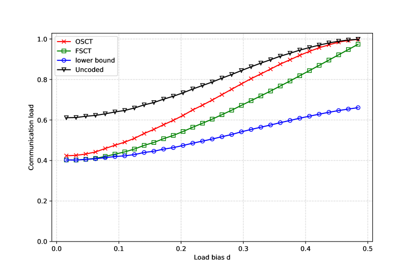
Figure 1: Comparison of communication load achieved by OSCT and FSCT with lower bound in systems with mapping load $\mathbf{m}=(\frac{1}{2}-d,\frac{1}{2}-d,\frac{1}{2}+d,\frac{1}{2}+d)$ and reducing load $(\frac{1}{2}+d,\frac{1}{2}+d,\frac{1}{2}-d,\frac{1}{2}-d)$

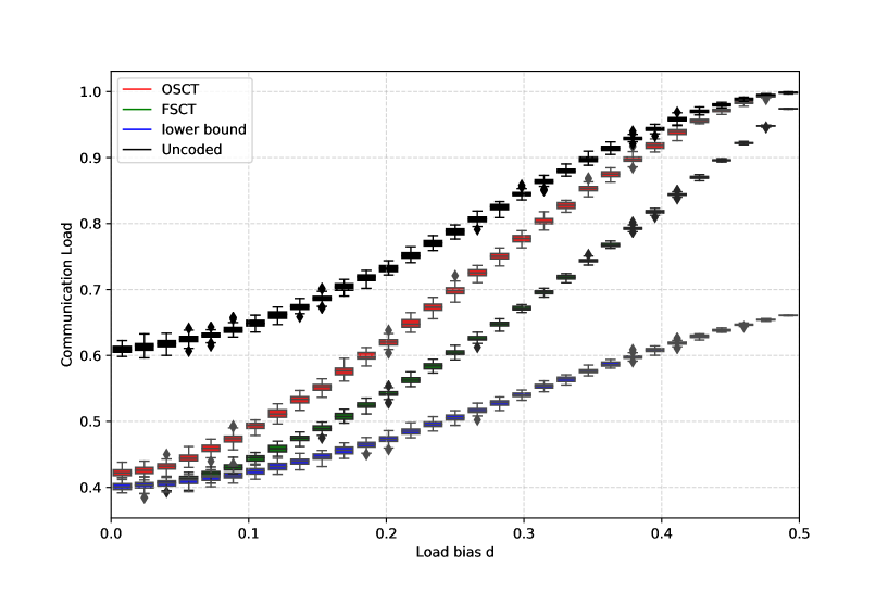
Figure 2: Boxplot of communication loads corresponding to OSCT (red color), FSCT (yellow color), and lower bound (blue color) among 50 samples for each $d$.

IV Examples of OSCT and FSCT

In this section, we present two examples to illustrate the proposed OSCT and FSCT. To simplify notations, we use $v_{[a:b],m}$ $a,b,m\in\mathbb{Z}^{+}$ to denote the set of IVs $\{v_{q,n}:a\leq q\leq b,n=m\}$.

IV-A Example 1: OSCT

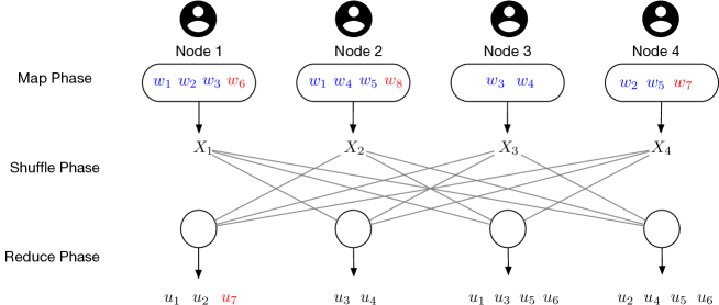
Figure 3: Data allocation and Reduce function assignment of Example 1

Consider the example with 4 nodes, 8 files and 7 Reduce functions. The file and Reduce function allocations are shown in Fig. 3.

Method illustration: In the Map phase, each node computes the IVs based on its local input files. Take node 3 as an example, it will get $v_{[1:7],3},v_{[1:7],4}$, totally 14 IVs.

In the Shuffle phase, as shown in Table II, we first regroup the nodes into different clusters $\mathcal{S}\subseteq[K]$ of size $\max\{r_{\min}+1,q_{\min}\}\leq|\mathcal{S}|\leq\min\{K,r_{\min}+q_{\min}\}$. In this example, IVs are communicated within each cluster of $2$, $3$, and $4$ nodes respectively. The sending process in each cluster $\mathcal{S}$ is further divided into multiple rounds, indexed as $z\in\{r_{\min},r_{\min}+1,\cdots,|\mathcal{S}|-1\}$, where the IVs in $(z,\mathcal{S})$-mapped set $\mathcal{V}_{z}^{\mathcal{S}}$ will be sent in round $z$ of cluster $\mathcal{S}$. We can skip the round $z$ if there exists no file mapped by exactly $z$ nodes in $\mathcal{S}$.

For example, in round $z=2$ of cluster $\mathcal{S}=\{1,2,3\}$, all IVs in the $(2,\{1,2,3\})$-mapped IVs set, i.e., $\mathcal{V}_{\{1,2\}}^{\{3\}}=\{v_{1,1},v_{3,1}\}$, $\mathcal{V}_{\{1,3\}}^{\{2\}}=\{v_{3,3}\}$, and $\mathcal{V}_{\{2,3\}}^{\{1\}}=\{v_{1,4},v_{7,4}\}$, will be encoded and delivered. Recall that IVs in $\mathcal{V}_{\{1,2\}}^{\{3\}}=\{v_{1,1},v_{3,1}\}$ are jointly mapped by nodes in $\{1,2\}$ and required by Node $3$. See the complete categories of IVs in all clusters and rounds in Table II.

TABLE II: Optimal $(\boldsymbol{\alpha}_{z}^{\mathcal{S}})^{*}$ of all the clusters and rounds in Example 1

Cluster	Round	IVs	$\alpha_{i,z}^{\mathcal{S}}$	Cluster	Round	IVs	$\alpha_{i,z}^{\mathcal{S}}$
{1,2,3,4}	2	$v_{5,1},v_{6,1},v_{4,3},v_{3,2},v_{2,4},v_{1,5}$	$(1,1,0,0)$	{2,3,4}	1	$v_{5,8},v_{6,8},v_{3,7}$	$(2,0,1)$
{1,2,3}	2	$v_{1,1},v_{3,1},v_{3,3},v_{1,4},v_{7,4}$	$(\frac{1}{2},\frac{3}{2},\frac{1}{2})$	{1,2}	1	$v_{7,8}$	$(0,1)$
	1	$v_{3,6},v_{1,8}$	$(1,1,0)$	{1,3}	1	$v_{1,6}$	$(1,0)$
{1,2,4}	2	$v_{2,1},v_{4,1},v_{4,2},v_{2,5},v_{7,5}$	$(1,1,0)$	{1,4}	1	$v_{2,6},v_{2,7},v_{7,7}$	$(1,2)$
	1	$v_{4,6},v_{2,8}$	$(1,1,0)$	{2,3}	1	$v_{3,8}$	$(1,0)$
{1,3,4}	2	$v_{2,3},v_{5,3},v_{6,3},v_{1,2},v_{5,2},v_{6,2}$	$(3,0,0)$	{2,4}	1	$v_{4,8},v_{4,7}$	$(1,1)$
	1	$v_{5,6},v_{6,6},v_{1,5}$	$(2,0,1)$	{3,4}	1	$v_{5,7},v_{6,7}$	$(0,2)$
{2,3,4}	2	$v_{4,4},v_{5,4},v_{6,4},v_{3,5},v_{5,5},v_{6,5}$	$(3,0,0)$

In each sending cluster $\mathcal{S}$ and round $z$, we first solve $\mathcal{P}(z,\mathcal{S})$ in Theorem 1 to obtain $\alpha_{j,z}^{\mathcal{S}}$ for all $j\in\mathcal{S}$. See the solutions for all clusters and rounds in Table II. For round $2$ of $\{1,2,3\}$, according to Remark 1, we can get $\alpha_{1,2}^{\{1,2,3\}}=\frac{1}{2}$, $\alpha_{2,2}^{\{1,2,3\}}=\frac{3}{2}$, and $\alpha_{3,2}^{\{1,2,3\}}=\frac{1}{2}$ directly from (8), since the deficit ratios of all the three nodes are less than $\frac{3-2}{2-1}=1$.

Based on the solution $\alpha_{j,z}^{\mathcal{S}}$, IVs in each set $\mathcal{V}_{\mathcal{S}_{1}}^{\mathcal{S}\backslash\mathcal{S}_{1}}$ for $\mathcal{S}_{1}\subset\mathcal{S}$ and $|\mathcal{S}_{1}|=z$ are concatenated and split into $z$ segments. For example, since IVs in $\mathcal{V}_{\{1,2\}}^{\{3\}}=\{v_{1,1},v_{3,1}\}$ are jointly mapped by Node $1$ and $2$, we evenly split $v_{1,1}$ into $v_{1,1}^{(1)}$ and $v_{1,1}^{(2)}$, where $v_{1,1}^{(1)}$ with size of $\alpha_{1,2}^{\{1,2,3\}}V=\frac{1}{2}V$ bits will be encoded by Node $1$ while $(v_{1,1}^{(2)},v_{3,1})$ with size of $\alpha_{2,2}^{\{1,2,3\}}V=\frac{3}{2}V$ bits will be encoded by Node $2$. We list all the split IV segments in round $2$ of cluster $\{1,2,3\}$ in Table III.

TABLE III: Split IV segments based on the solution of $\{\alpha_{j,z}^{\mathcal{S}}\}_{j\in\mathcal{S}}$ in round $2$ of cluster $\{1,2,3\}$.

	$\alpha_{1,2}^{\{1,2,3\}}V$	$\alpha_{2,2}^{\{1,2,3\}}V$	$\alpha_{3,2}^{\{1,2,3\}}V$
$\mathcal{V}_{\{1,2\}}^{\{3\}}\!\!=\!\!\{v_{1,1},v_{3,1}\}$	$v_{1,1}^{(1)}$	$v_{1,1}^{(2)},v_{3,1}$
$\mathcal{V}_{\{1,3\}}^{\{2\}}\!\!=\!\!\{v_{3,3}\}$	$v_{3,3}^{(1)}$		$v_{3,3}^{(2)}$
$\mathcal{V}_{\{2,3\}}^{\{1\}}\!\!=\!\!\{v_{1,4},v_{7,4}\}$		$v_{1,4}^{(1)},v_{7,4}$	$v_{1,4}^{(2)}$

Then each node encodes the corresponding segments into linear combinations. In round $2$ of cluster $\{1,2,3\}$, Node 2 multicasts $(v_{1,1}^{(2)}\oplus v_{1,4}^{(1)},v_{3,1}\oplus v_{7,4})$ to Node 1 and Node 3. Node 1 multicasts $v_{1,1}^{(1)}\oplus v_{3,3}^{(1)}$ to Node 2 and Node 3, and Node 3 multicasts $v_{3,3}^{(2)}\oplus v_{1,4}^{(2)}$ to Node 1 and Node 2, as shown in Fig. 4. Note that each node can successfully decode its desired IVs from the received messages. For example, as Node 1 knows $v_{1,1}^{(2)},v_{3,1}$ and Node 3 knows $v_{3,3}^{(1)},v_{7,4}$, both of them can decode the messages $(v_{1,1}^{(2)}\oplus v_{1,4}^{(1)},v_{3,1}\oplus v_{7,4})$ sent by Node 2.

Following the similar approaches to send all other $(z,S)$-mapped IVs with parameters $\alpha_{j,z}^{\mathcal{S}}$ in Table II, we can obtain the communication load given by OSCT is $L_{\textnormal{OSCT}}=\frac{35}{56}$. Some examples of the encoded messages sent in other clusters are listed in Table IV.

TABLE IV: Some encoded messages sent by each node in data shuffle phase in Example 1

Cluster	Round	Node 1	Node 2	Node 3	Node 4
{1,2,3,4}	2	$v_{5,1}+v_{4,3}+v_{3,2}$ $a_{1}v_{5,1}+a_{2}v_{4,3}+a_{3}v_{3,2}$	$v_{6,1}+v_{2,4}+v_{1,5}$ $a_{1}v_{6,1}+a_{2}v_{2,4}+a_{3}v_{1,5}$
{1,2,3}	1	$v_{3,6}$	$v_{1,8}$
{1,2,3}	2	$v_{1,1}^{(1)}\oplus v_{3,3}^{(3)}$	$v_{1,1}^{(2)}\oplus v_{1,4}^{(1)}$ $v_{3,1}^{(1)}\oplus v_{7,4}^{(1)}$ $v_{3,1}^{(2)}\oplus v_{7,4}^{(2)}$	$v_{1,2}^{(1)}\oplus v_{3,3}^{(2)}$
{1,4}	1	$v_{2,6}$			$v_{2,7},v_{7,7}$
$\ldots$	$\ldots$	$\ldots$	$\ldots$	$\ldots$	$\ldots$

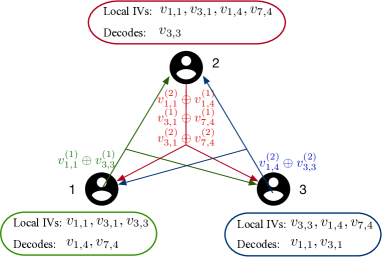
Figure 4: Illustration of Shuffle phase of OSCT in round $2$ of cluster $\{1,2,3\}$ in Example 1.

Comparison with previous schemes: For the scheme proposed in [23], the data allocation and Reduce function assignment in this example are fixed and do not follow the combinatorial design in [23], in which each file and Reduce function are required to be mapped or computed exactly $r$ times. Thus, their Shuffle phase design is not applicable in this example.

For the scheme in [24], by solving the optimization problem in [24, Theorem 1] with Mapping load $({m}_{1},\ldots,m_{4})=\left(\frac{1}{2},\frac{1}{2},\frac{1}{4},\frac{3}{8}\right)$ and Reducing load $(\omega_{1},\ldots,\omega_{4})=\left(\frac{3}{7},\frac{2}{7},\frac{4}{7},\frac{4}{7}\right)$, we can obtain that the total communication load is $\frac{3}{112}+$$\frac{5}{112}+$$\frac{1}{112}+$ $\frac{3}{112}+$$\frac{5}{112}+$$\frac{1}{112}+$$\frac{1}{14}+$$\frac{1}{14}=$$\frac{47}{56}$, which is larger than OSCT.

According to Lemma 1, the theoretical lower bound of communication load for this system is $L^{*}=\frac{35}{56}=L_{\textnormal{OSCT}}$, which means our OSCT is optimal.

IV-B Example 2: FSCT

Consider another example with 4 nodes, 7 files and 6 Reduce functions. The file and Reduce function allocations are shown in Fig. 5. Now we show how to use our FSCT to achieve the optimal communication load in this specific system.

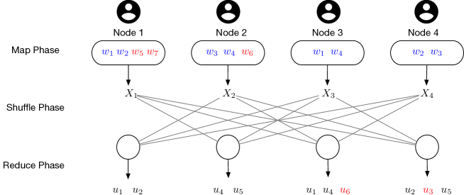
Figure 5: Data allocation and Reduce function assignment of Example 2.

Method illustration: First, we perform the same steps as in Example 1 to regroup the nodes into clusters and divide the sending process into multiple rounds for each cluster. The IVs in $(z,\mathcal{S})$-mapped set $\mathcal{V}_{z}^{\mathcal{S}}$ will be sent in round $z$ of cluster $\mathcal{S}$.

Then in each round, we check whether the deficit condition and feasible condition defined in (11) and (13) are satisfied for each node. Taking round 2 of cluster $\{1,2,3,4\}$ as an example, the IVs categories are shown in Table V. According to (10), we obtain that $n_{1,2}^{\{1,2,3,4\}}=n_{2,2}^{\{1,2,3,4\}}=n_{3,2}^{\{1,2,3,4\}}=n_{4,2}^{\{1,2,3,4\}}=2>0$, which satisfies the deficit conditions for all nodes by checking (12). One can verify that all nodes also satisfy the feasible conditions. For example, $\beta_{2,\{2,3\}}=\beta_{3,\{2,3\}}=\beta_{2,\{2,4\}}=\beta_{4,\{2,4\}}=1,\beta_{3,\{3,4\}}=\beta_{4,\{3,4\}}=0$ is a non-negative solution of (13) for Node 1.

Then each IV sent in round $z$ of cluster $S$ will be splitted into $|\mathcal{S}|-1$ pieces, and each node who satisfies both the deficit condition and feasible condition encodes all locally mapped IVs in this round into a message with $n_{i,z}^{\mathcal{S}}$ LCs, where $n_{i,z}^{\mathcal{S}}$ is the parameter introduced in (10). For example, each IV in round 2 of $\{1,2,3,4\}$ will be splitted into $|\mathcal{S}|-1=3$ pieces, (e.g., $V_{5,1}$ is splitted into $v_{5,1}^{(1)},v_{5,1}^{(2)}$ and $v_{5,1}^{(3)}$). Node 1 maps IVs in $\mathcal{V}_{\{1,2\}}^{\{3,4\}}$, $\mathcal{V}_{\{1,3\}}^{\{2,4\}}$ and $\mathcal{V}_{\{1,4\}}^{\{2,3\}}$, so it knows IVs segments of $\{v_{5,1}^{(1)}$, $v_{4,2}^{(1)}$, $v_{5,1}^{(2)},v_{4,2}^{(2)},v_{5,1}^{(3)},v_{4,2}^{(3)}\}$. Then, Node 1 multicasts $n_{1,2}^{\{1,2,3,4\}}=2$ linear combinations (LCs) of $v_{5,1}^{(1)}$, $v_{4,2}^{(1)}$, $v_{5,1}^{(2)},v_{4,2}^{(2)},v_{5,1}^{(3)},v_{4,2}^{(3)}$ as follow

$$v_{5,1}^{(1)}+v_{4,2}^{(1)}+v_{5,1}^{(2)}+v_{4,2}^{(2)}+v_{5,1}^{(3)}+v_{4,2}^{(3)},$$

$$a_{1}v_{5,1}^{(1)}+a_{2}v_{4,2}^{(1)}+a_{3}v_{5,1}^{(2)}+a_{4}v_{4,2}^{(2)}+a_{5}v_{5,1}^{(3)}+a_{6}v_{4,2}^{(3)},$$

where $a_{i}\in\mathbb{F}_{2^{\frac{V}{|\mathcal{S}|-1}}}$ for $i\in[6]$ is the randomly generated coefficient.

TABLE V: IVs categories in cluster $\{1,2,3,4\}$ for example 2

$\mathcal{V}_{\{1,2\}}^{\{3,4\}}$	$\mathcal{V}_{\{1,3\}}^{\{2,4\}}$	$\mathcal{V}_{\{1,4\}}^{\{2,3\}}$	$\mathcal{V}_{\{2,3\}}^{\{1,4\}}$	$\mathcal{V}_{\{2,4\}}^{\{1,3\}}$	$\mathcal{V}_{\{3,4\}}^{\{1,2\}}$
$\emptyset$	$v_{5,1}$	$v_{4,2}$	$v_{2,4}$	$v_{1,3}$	$\emptyset$

Coded shuffle strategies for Node 2, 3, and 4 are shown below:

• Node 2 multicasts 2 LCs of $v_{2,4}^{(1)}$, $v_{1,3}^{(1)}$, $v_{2,4}^{(2)}$, $v_{1,3}^{(2)}$, $v_{2,4}^{(3)}$, $v_{1,3}^{(3)}$.

• Node 3 multicasts 2 LCs of $v_{5,1}^{(1)}$, $v_{2,4}^{(1)}$, $v_{5,1}^{(2)}$, $v_{2,4}^{(2)}$, $v_{5,1}^{(3)}$, $v_{2,4}^{(3)}$.

• Node 4 multicasts 2 LCs of $v_{4,2}^{(1)}$, $v_{1,3}^{(1)}$, $v_{4,2}^{(2)}$, $v_{1,3}^{(2)}$, $v_{4,2}^{(3)}$, $v_{1,3}^{(3)}$.

Although each node can not decode the desired IVs directly from a single message block, each node can jointly solve its needed IVs segments after receiving all the LCs in round $z$ of cluster $\mathcal{S}$. For example, Node 1 receives 6 LCs of total of 12 segments from the other 3 nodes in round 2 of cluster $\{1,2,3,4\}$. After removing its known segments $\{v_{5,1}^{(1)}$, $v_{4,2}^{(1)}$, $v_{5,1}^{(2)},v_{4,2}^{(2)},v_{5,1}^{(3)},v_{4,2}^{(3)}\}$, Node 1 will solve a linear system with 6 independent linear combinations of its 6 desired segments $v_{2,4}^{(1)}$, $v_{1,5}^{(1)}$, $v_{2,4}^{(2)}$, $v_{1,5}^{(2)}$, $v_{2,4}^{(3)}$, $v_{1,5}^{(3)}$.

Comparison with OSCT and previous schemes: For the scheme proposed in [23], the data placement and Reduce function assignment in this example are fixed and do not follow their combinatorial design, in which each file and each Reduce function are required to be mapped or computed exactly $r$ times. Thus, their Shuffle phase design is not applicable in this example.

For the scheme in [24], by solving the optimization problem in [24, Theorem 1] with the Mapping load $(m_{1},\ldots,m_{4})=\left(\frac{4}{7},\frac{3}{7},\frac{2}{7},\frac{2}{7}\right)$ and Reducing load $(\omega_{1},\ldots,\omega_{4})=\left(\frac{1}{3},\frac{1}{3},\frac{1}{2},\frac{1}{2}\right)$, we can get the total communication load as $\frac{32}{42}=0.762$.

For our FSCT, as the deficit condition and feasible condition are satisfied by all the nodes in every cluster, the communication load is $L_{\textnormal{fsct}}=0.635$ according to Theorem 3. According to Lemma 1, the theoretical lower bound of the communication load is $L^{*}=0.635=L_{\textnormal{fsct}}$, which means that FSCT is optimal.

According to Theorem 1, the upper bound of communication load given by OSCT is $L_{\textnormal{OSCT}}=\frac{28}{42}=0.667$, smaller than that of [24], but larger than $0.635$ (i.e., not optimal). From this example, we see that FSCT outperforms OSCT by jointly decoding multiple message blocks.

V One-Shot Coded Transmission (Proof of Theorem 1)

The key idea of OSCT is to exploit the gain of multicasting by grouping nodes into clusters with different sizes and carefully categorizing IVs, and then precisely designing the size of messages sent by every node in each cluster. More specifically, we first group the nodes into different clusters $\mathcal{S}\subseteq[K]$ of size $\max\{r_{\min}+1,q_{\min}\}\leq|\mathcal{S}|\leq\min\{K,r_{\min}+q_{\min}\}$ and divide the sending process in each cluster $\mathcal{S}$ into multiple rounds, indexed as $z\in\{r_{\min},r_{\min}+1,\cdots,|\mathcal{S}|-1\}$. The intermediate values in $\mathcal{V}_{\mathcal{S}_{z}[i]}^{\mathcal{S}\backslash\mathcal{S}_{z}[i]},$ for all $i\in\left[\binom{|\mathcal{S}|}{z}\right]$ will be sent in round $z$ by messages of different sizes determined by solving an optimization problem.

V-A Definitions of Sending Clusters and Rounds

Note that after the Map phase, Node $k\in[K]$ has obtained its local IVs $\{v_{q,n}:q\in[Q],n\in\mathcal{M}_{k}\}$, and it requires IVs in

$$\{v_{q,n}:q\in\mathcal{W}_{k},n\notin\mathcal{M}_{k}\}.$$ (22)

Given the pre-set $\mathcal{M}$ and $\mathcal{W}$, first compute the minimum Mapping times $r_{\textnormal{min}}=\min\limits_{1\leq i\leq N}r_{i}$ and the minimum Reducing times $q_{\textnormal{min}}=\min\limits_{1\leq i\leq Q}q_{i}$. We call each subset $\mathcal{S}\subseteq[K]$ of size $\max\{r_{\min}+1,q_{\min}\}\leq|\mathcal{S}|\leq\min\{K,r_{\min}+q_{\min}\}$ a sending cluster. For each sending cluster $\mathcal{S}$, any file $w_{n}$ exclusively stored by nodes in $\mathcal{S}$, i.e., $n\in\cup_{k\in\mathcal{S}}\mathcal{M}_{k},n\notin\cup_{k\in[K]\backslash\mathcal{S}}\mathcal{M}_{k},$ is possibly stored by $z\in\{r_{\text{min}},r_{\text{min}}+1,\ldots,|\mathcal{S}|\}$ nodes in $\mathcal{S}$. Thus, we divide the sending process into multiple rounds, indexed as $z\in\{r_{\min},r_{\text{min}}+1,\cdots,|\mathcal{S}|-1\}$. The round $z$ is skipped if there exists no file in $(z,\mathcal{S})$-mapped IVs. For example, Table IV lists the clusters and rounds in a four-node system, where Round 1 and Round 3 of Cluster $\{1,2,3,4\}$ are skipped since no intermediate value is mapped by $3$ nodes or reduced by $3$ nodes.

In round $z$, there are $\binom{|\mathcal{S}|}{z}$ subsets of $\mathcal{S}$ of size $z$, namely, $\mathcal{S}_{z}[1],\mathcal{S}_{z}[2],\cdots,\mathcal{S}_{z}[\binom{|\mathcal{S}|}{z}]$. According to the definition in (2), we can write the set of IVs needed by all nodes in $\mathcal{S}\backslash\mathcal{S}_{z}[i]$, no nodes outside $\mathcal{S}$, and known exclusively by nodes in $\mathcal{\mathcal{missing}}S_{z}[i]$ as $\mathcal{V}_{\mathcal{S}_{z}[i]}^{\mathcal{S}\backslash\mathcal{S}_{z}[i]}$ for $i\in\left[\binom{|\mathcal{S}|}{z}\right]$, i.e.,

$$\mathcal{V}_{\mathcal{S}_{z}[i]}^{\mathcal{S}\backslash\mathcal{S}_{z}[i]} = \{v_{q,n}:q\in\underset{k\in\mathcal{S}\backslash{S}_{z}[i]}{\cap}{\mathcal{W}}_{k},q\notin\underset{k\notin\mathcal{S}}{\cup}{\mathcal{W}}_{k},n\in\underset{k\in{S}_{z}[i]}{\cap}\mathcal{M}_{k},n\notin\underset{k\notin{S}_{z}[i]}{\cup}{\mathcal{M}}_{k}\}.\qquad\quad$$ (23)

Then, the $(z,\mathcal{S})$-mapped IVs in can be written as $\mathcal{V}_{z}^{\mathcal{S}}=\bigcup_{i=1}^{\binom{|\mathcal{S}|}{z}}\mathcal{V}_{\mathcal{S}_{z}[i]}^{\mathcal{S}\backslash\mathcal{S}_{z}[i]}$. As we will see, all IVs in $\mathcal{V}_{\mathcal{S}_{z}[i]}^{\mathcal{S}\backslash\mathcal{S}_{z}[i]}$ will be jointly sent out by the $z$ nodes in $\mathcal{S}_{z}[i]$ and all IVs in $\mathcal{V}_{z}^{\mathcal{S}}$ will be sent in round $z$ of cluster $\mathcal{S}$. Since the sizes of $\mathcal{V}_{\mathcal{S}_{z}[i]}^{\mathcal{S}\backslash\mathcal{S}_{z}[i]}$ for $i\in[\binom{|\mathcal{S}|}{z}]$ are not necessarily equal, we can not simply partition each IVs set into $z$ parts and let each node send one part. Instead, we design an optimization-based transmission strategy as follows to determine the size of each message.

V-B Transmission Strategy of OSCT

In each sending cluster $\mathcal{S}$ and round $z$, introduce a parameter vector $\boldsymbol{\alpha}_{z}^{S}=(\alpha^{S}_{j,z}:j\in\mathcal{S})$ in the descending order of $j$, where $\{\alpha^{S}_{j,z}\}$ is the solution to the problem in $\mathcal{P}_{\textnormal{OSCT}}(\mathcal{S},z)$ present in Theorem 1. For convenience, we rewrite $\mathcal{P}_{\textnormal{OSCT}}(\mathcal{S},z)$ here:

$$\min_{\alpha_{j,z}^{\mathcal{S}}}\sum_{i=1}^{\binom{|\mathcal{S}|}{z}}\Big{(}\left|\mathcal{V}_{\mathcal{S}_{z}[i]}^{\mathcal{S}\backslash\mathcal{S}_{z}[i]}\right|-\sum_{j\in\mathcal{S}_{z}[i]}\alpha_{j,z}^{\mathcal{S}}\Big{)}^{2}$$ (7a)

$$\quad{s.t.}~{}\alpha_{j,z}^{\mathcal{S}}\in\mathbb{Q}^{+},\forall j\in\mathcal{S}$$ (7b)

$$\ \ \ \ \ \ \sum_{j\in\mathcal{\mathcal{missing}}S_{z}[i]}\alpha_{j,z}^{\mathcal{S}}=0,\ \text{if}\ |\mathcal{V}_{\mathcal{S}_{z}[i]}^{\mathcal{S}\backslash\mathcal{S}_{z}[i]}|=0,\forall i\in\left[\tbinom{|\mathcal{S}|}{z}\right].$$ (7c)

Let

$$\tau_{i,z}^{\mathcal{S}}\triangleq\left|\mathcal{V}_{\mathcal{S}_{z}[i]}^{\mathcal{S}\backslash\mathcal{S}_{z}[i]}\right|-\sum_{j\in\mathcal{S}_{z}[i]}\alpha_{j,z}^{\mathcal{S}},~{}\forall i\in[\tbinom{|\mathcal{S}|}{z}].$$

We first concatenate all IVs in $\mathcal{V}_{\mathcal{S}_{z}[i]}^{\mathcal{S}\backslash\mathcal{S}_{z}[i]}$ to construct a symbol $U_{\mathcal{S}_{z}[i]}^{\mathcal{S}\backslash\mathcal{S}_{z}[i]}$, and then split $U_{\mathcal{S}_{z}[i]}^{\mathcal{S}\backslash\mathcal{S}_{z}[i]}$ as follows.

If ${\tau}_{i,z}^{\mathcal{S}}\leq 0$, concatenate extra $|{\tau}_{i,z}^{\mathcal{S}}|\cdot V$ bits of 0 to the end of $U_{\mathcal{S}_{z}[i]}^{\mathcal{S}\backslash\mathcal{S}_{z}[i]}$, and then split $U_{\mathcal{S}_{z}[i]}^{\mathcal{S}\backslash\mathcal{S}_{z}[i]}$ into $z$ segments, i.e.,

$$U_{\mathcal{S}_{z}[i]}^{\mathcal{S}\backslash\mathcal{S}_{z}[i]}\!=\!\left({U}_{\mathcal{S}_{z}[i],\sigma_{1}}^{\mathcal{S}\backslash\mathcal{S}_{z}[i]},{U}_{\mathcal{S}_{z}[i],\sigma_{2}}^{\mathcal{S}\backslash\mathcal{S}_{z}[i]},\cdots,{U}_{\mathcal{S}_{z}[i],\sigma_{z}}^{\mathcal{S}\backslash\mathcal{S}_{z}[i]}\right),\quad$$ (24)

where ${U}_{\mathcal{S}_{z}[i],\sigma_{j}}^{\mathcal{S}\backslash\mathcal{S}_{z}[i]}\in\mathbb{F}_{2^{(\alpha^{\mathcal{S}}_{\sigma_{j},z})V}}$ and $\sigma_{j}\in\mathcal{S}_{z}[i]$, for $j\in[z]$. Note that, unlike the original CDC scheme where each segment has equal size, here each segment ${U}_{\mathcal{S}_{z}[i],\sigma_{j}}^{\mathcal{S}}$ is of size $(\alpha^{\mathcal{S}}_{\sigma_{j},z})V$ bits, determined by solution to the optimization problem $\mathcal{P}_{\textnormal{OSCT}}(\mathcal{S},z)$. If ${\tau}_{i,z}^{\mathcal{S}}>0$, we directly split $U_{\mathcal{S}_{z}[i]}^{\mathcal{S}\backslash\mathcal{S}_{z}[i]}$ (without any 0 concatenated at the end) into $z+1$ segments. The first $z$ segments are the same as (24) (i.e., with size of $(\alpha^{\mathcal{S}}_{\sigma_{j},z})V$ bits for each $\sigma_{j}\in\mathcal{S}_{z}[i]$, $j\in[z]$), and the $(z+1)$-th segment is ${U}_{{\tau}_{i,z}^{\mathcal{S}}>0}\in\mathbb{F}_{2^{({\tau}_{i,z}^{\mathcal{S}})V}}$, i.e.,

$$U_{\mathcal{S}_{z}[i]}^{\mathcal{S}\backslash\mathcal{S}_{z}[i]}\!=\!\left({U}_{\mathcal{S}_{z}[i],\sigma_{1}}^{\mathcal{S}\backslash\mathcal{S}_{z}[i]},{U}_{\mathcal{S}_{z}[i],\sigma_{2}}^{\mathcal{S}\backslash\mathcal{S}_{z}[i]},\cdots,{U}_{\mathcal{S}_{z}[i],\sigma_{z}}^{\mathcal{S}\backslash\mathcal{S}_{z}[i]},{U}_{{\tau}_{i,z}^{\mathcal{S}}>0}\right).\quad$$ (25)

Here $\alpha_{\sigma_{j},z}^{\mathcal{S}}V$ represents the size of segment ${U}_{\mathcal{S}_{z}[i],\sigma_{j}}^{\mathcal{S}\backslash\mathcal{S}_{z}[i]}$, and thus must be non-negative, leading to the constraint (7b) in $\mathcal{P}_{\textnormal{OSCT}}(\mathcal{S},z)$. Besides, if the $|\mathcal{V}_{\mathcal{S}_{z}[i]}^{\mathcal{S}\backslash\mathcal{S}_{z}[i]}|=0$, then the size of each splitted segments $|U_{\mathcal{S}_{z}[i],\sigma_{j}}^{\mathcal{S}\backslash\mathcal{S}_{z}[i]}|=0$, so the corresponding $\alpha_{\sigma_{j},z}^{\mathcal{S}}$ for $\sigma_{j}\in\mathcal{S}_{z}[i]$ is 0, leading to the condition (7c) in $\mathcal{P}_{\textnormal{OSCT}}(\mathcal{S},z)$. In other words, this constraint guarantees that $z$ nodes in $\mathcal{S}_{z}[i]$ will jointly map at least one IV, otherwise the corresponding $\alpha_{\sigma_{j},z}^{\mathcal{S}}$ for $\sigma_{j}\in\mathcal{S}_{z}[i]$ will be set to 0 in this round.

In the following, we present how to deliver all segments in (24) or (25).

V-B1 Encoding

If ${\tau}_{i,z}^{\mathcal{S}}>0$, the $(z+1)$-th segment ${U}_{{\tau}_{i,z}^{\mathcal{S}}>0}\in\mathbb{F}_{2^{(\tau_{i,z}^{\mathcal{S}})V}}$ in (25) is directly unicasted by an arbitrary node in $\mathcal{S}_{z}[i]$ to the nodes in $\mathcal{S}\backslash\mathcal{S}_{z}[i]$.

For segments in (24) or the first $z$ segments in (25), i.e., $U_{\mathcal{S}_{z}[i],\sigma_{j}}^{\mathcal{S}\backslash\mathcal{S}_{z}[i]}$ for $i\in\left[\binom{|\mathcal{S}|}{z}\right]$, $j\in[z]$, Node $k\in\mathcal{S}$ encodes the segment vector $\mathbf{u}_{k,z}^{\mathcal{S}}=\left({U}_{\mathcal{S}_{z}[i],k}^{\mathcal{S}\backslash\mathcal{S}_{z}[i]}:i\in\left[\tbinom{|\mathcal{S}|}{z}\right],k\in\mathcal{S}_{z}[i]\right)$ including $\binom{|\mathcal{S}|-1}{z-1}$ segments each of size $(\alpha_{k,z}^{\mathcal{S}})V$ bits, into $\binom{|\mathcal{S}|-2}{z-1}$ numbers of LCs. Specifically, Node $k$ multicasts a message block $\left(X_{k,z}^{\mathcal{S}}[{1}],X_{k,z}^{\mathcal{S}}[{2}],\cdots,X_{k,z}^{\mathcal{S}}[{\binom{|\mathcal{S}|-2}{z-1}}]\right)$ as follows:

$$\begin{bmatrix}X_{k,z}^{\mathcal{S}}[1]\\ X_{k,z}^{\mathcal{S}}[2]\\ \vdots\\ X_{k,z}^{\mathcal{S}}[\binom{|\mathcal{S}|-2}{z-1}]\end{bmatrix}\!=\!{\mathbf{V}}_{z}\cdot\mathbf{u}_{k,z}^{\mathcal{S}},$$ (26)

where

$${\mathbf{V}}_{z}=\begin{bmatrix}\!1&1&\cdots&1\\ v_{1}&v_{2}&\cdots&v_{\binom{|\mathcal{S}|-1}{z-1}}\\ \vdots&\vdots&\ddots&\vdots\\ v_{1}^{\binom{|\mathcal{S}|-2}{z-1}-1}&v_{2}^{\binom{|\mathcal{S}|-2}{z-1}-1}&\cdots&v_{\binom{|\mathcal{S}|-1}{z-1}}^{\binom{|\mathcal{S}|-2}{z-1}-1}\!\end{bmatrix}$$

is a Vandermonde matrix for some coefficients $v_{j}\in\mathbb{F}_{2^{(\alpha^{\mathcal{S}}_{k,z})V}}$, $j\in[\binom{|\mathcal{S}|-1}{z-1}]$.

Apply the above encoding process to send all IVs in $\bigcup_{z=r_{\min}}^{|\mathcal{S}|-1}\mathcal{V}_{z}^{\mathcal{S}}$ in sending cluster $\mathcal{S}\subseteq[K]$, where $\mathcal{V}_{z}^{\mathcal{S}}$ is the $(z,\mathcal{S})$-mapped IVs defined in (3).

V-B2 Decoding

In each sending cluster $\mathcal{S}$ and round $z$, after receiving the message block from Node $k$: $\big{(}X_{k,z}^{\mathcal{S}}[{1}],X_{k,z}^{\mathcal{S}}[{2}],\cdots,$ $X_{k,z}^{\mathcal{S}}[{\binom{|\mathcal{S}|-2}{z-1}}]\big{)}$, Node $j\in\mathcal{S}$ with $j\neq k$ decodes its desired segments $\Big{\{}{U}_{\mathcal{S}_{z}[i],k}^{\mathcal{S}\backslash\mathcal{S}_{z}[i]}:i\in\left[\binom{|\mathcal{S}|}{z}\right],k\in\mathcal{S}_{z}[i],j\notin\mathcal{S}_{z}[i]\Big{\}}$ based on the local segments $\Big{\{}{U}_{\mathcal{S}_{z}[i],k}^{\mathcal{S}\backslash\mathcal{S}_{z}[i]}:i\in\left[\binom{|\mathcal{S}|}{z}\right],k,j\in\mathcal{S}_{z}[i]\Big{\}}$. Following the similar steps in [5], Node $j$ first removes the local segments from the received LCs and then decodes the desired segments by multiplying an invertible Vandermonde matrix.

V-B3 Correctness of the Scheme

Now we show that each Node $j\in\mathcal{S}\backslash\{k\}$ can decode its desired segments after receiving the block message sent from Node $k$: $\Big{(}X_{k,z}^{\mathcal{S}}[{1}],X_{k,z}^{\mathcal{S}}[{2}],\cdots,X_{k,z}^{\mathcal{S}}[{\binom{|\mathcal{S}|-2}{z-1}}]\Big{)}$. Among all segments generating $\Big{(}X_{k,z}^{\mathcal{S}}[{1}],X_{k,z}^{\mathcal{S}}[{2}],\cdots,$ $X_{k,z}^{\mathcal{S}}[{\binom{|\mathcal{S}|-2}{z-1}}]\Big{)}$, i.e., $\Big{\{}{U}_{\mathcal{S}_{z}[i],k}^{\mathcal{S}\backslash\mathcal{S}_{z}[i]}:i\in\Big{[}\binom{|\mathcal{S}|}{z}\Big{]},k\in\mathcal{S}_{z}[i]\Big{\}}$, there are $\binom{|\mathcal{S}|-2}{z-2}$ segments $\Big{\{}{U}_{\mathcal{S}_{z}[i],k}^{\mathcal{S}\backslash\mathcal{S}_{z}[i]}:i\in\Big{[}\binom{|\mathcal{S}|}{z}\Big{]},k,j\in\mathcal{S}_{z}[i]\Big{\}}$ already known by both Node $k$ and $j$, and $\binom{|\mathcal{S}|-1}{z-1}-\binom{|\mathcal{S}|-2}{z-2}=\binom{|\mathcal{S}|-2}{z-1}$ segments $\Big{\{}{U}_{\mathcal{S}_{z}[i],k}^{\mathcal{S}\backslash\mathcal{S}_{z}[i]}:i\in\big{[}\binom{|\mathcal{S}|}{z}\big{]},k\in\mathcal{S}_{z}[i],j\notin\mathcal{S}_{z}[i]\Big{\}}$ unknown by Node $j$. Constraint (7c) guarantees that all segments multicasted by Node $k$ and known by Node $j$ are not empty, i.e., $|{U}_{\mathcal{S}_{z}[i],k}^{\mathcal{S}\backslash\mathcal{S}_{z}[i]}|\neq 0$ for $i\in\Big{[}\binom{|\mathcal{S}|}{z}\Big{]},k,j\in\mathcal{S}_{z}[i]$. Thus, from $\binom{|\mathcal{S}|-2}{z-1}$ linearly independent combinations, Node $j$ can recover all $\binom{|\mathcal{S}|-2}{z-1}$ desired segments.

V-B4 Overall Communication Load

In round $z$ of cluster $\mathcal{S}$, Node $k$ multicasts $\binom{|\mathcal{S}|-2}{z-1}$ numbers of LCs, each of size $\alpha_{k,z}^{\mathcal{S}}V$ bits. Additionally, the segment ${U}_{{\tau}_{i,z}^{\mathcal{S}}>0}$, for $i\in\binom{|\mathcal{S}|}{z}$, of size ${\tau}_{i,z}^{\mathcal{S}}V$ bits is unicasted in this round if ${{\tau}_{i,z}^{\mathcal{S}}>0}$. So the communication cost in round $z$ of cluster $\mathcal{S}$ is:

$$L_{z,\mathcal{S}}=\sum_{k\in\mathcal{S}}\tbinom{|\mathcal{S}|-2}{z-1}\alpha_{k,z}^{\mathcal{S}}V+\sum_{i=1}^{\binom{|\mathcal{S}|}{z}}(\tau_{i,z}^{\mathcal{S}})^{+}V.$$ (27)

By considering all cluster $\mathcal{S}\subseteq[K]$ and all rounds $r_{\min}\leq z\leq|\mathcal{S}|-1$, and according to Definition 1, we obtain the overall communication load (normalized by $QNV$) of OSCT

$$L_{\textnormal{OSCT}} =\sum_{\mathcal{S}\subset[K]}\sum_{z=r_{\min}}^{|\mathcal{S}|-1}\frac{L_{z,\mathcal{S}}}{QNV}$$

$$=\frac{\sum\limits_{\mathcal{S}\subseteq[K]}\sum\limits_{z=r_{\min}}^{|\mathcal{S}|-1}\Big{(}\sum\limits_{k\in\mathcal{S}}\tbinom{|\mathcal{S}|-2}{z-1}\alpha_{k,z}^{\mathcal{S}}\!+\!\sum\limits_{i=1}^{\binom{|\mathcal{S}|}{z}}(\tau_{i,z}^{\mathcal{S}})^{+}\Big{)}}{QN}.$$ (28)

We call the approach above One-Shot Coded Transmission, since Node $k\in\mathcal{S}$ can decode its desired segments once Node $k$ receives a single message block $\left(X_{j,z}^{\mathcal{S}}[{1}],X_{j,z}^{\mathcal{S}}[{2}],\cdots,X_{j,z}^{\mathcal{S}}[{\binom{|\mathcal{S}|-2}{z-1}}]\right)$.

V-C Complexity of OSCT

For the OSCT strategy, consider the encoding and decoding processes of each node in round $z$ of cluster $\mathcal{S}$. As the multiplication of a $n\times n$ Vandermonde matrix and a vector can be done in $O\left(n\log^{2}n\right)$ time[45], the time complexity of encoding process is $O\big{(}\binom{|\mathcal{S}|-1}{z-1}\log^{2}\binom{|\mathcal{S}|-1}{z-1}\big{)}$ for each node in round $z$. There are $|\mathcal{S}|$ nodes in the cluster, and we sum the time complexity in every round and every cluster, then we have the total time complexity of the encoding process as

$$O\bigg{(}\sum_{\mathcal{S}\subseteq[K]}\sum_{z=r_{\min}}^{|\mathcal{S}|-1}|\mathcal{S}|\tbinom{|\mathcal{S}|-1}{z-1}\log^{2}\tbinom{|\mathcal{S}|-1}{z-1}\bigg{)}.$$ (29)

Similarly, as each node receives $|\mathcal{S}|-1$ message blocks from other nodes in round $z$ of cluster $\mathcal{S}$ and solving a linear system with $n$ equations requires $O(n^{3})$ time[46], the time complexity of decoding process is $\big{(}(|\mathcal{S}|-1)\binom{|\mathcal{S}|-2}{z-1}^{3}\big{)}$ for each node in round $z$. Totally, the complexity of the decoding process is

$$O\bigg{(}\sum_{\mathcal{S}\subseteq[K]}\sum_{z=r_{\min}}^{|\mathcal{S}|-1}|\mathcal{S}|(|\mathcal{S}|-1)\tbinom{|\mathcal{S}|-2}{z-1}^{3}\bigg{)}.$$ (30)

VI Few-Shot Coded Transmission (Proof of Theorem 3)

To further exploit the gain of multicasting, we propose the following FSCT strategy where each node wait to jointly decode multiple message blocks, leading to a potentially lower communication load at the cost of higher coding complexity.

Similar to OSCT, we group the nodes into different clusters $\mathcal{S}\subseteq[K]$ of size $\max\{r_{\min}+1,q_{\min}\}\leq|\mathcal{S}|\leq\min\{K,r_{\min}+q_{\min}\}$ and divide the sending process in each cluster $\mathcal{S}$ into multiple rounds, indexed as $z\in\{r_{\min},r_{\min}+1,\cdots,|\mathcal{S}|-1\}$. The intermediate values in $\mathcal{V}_{\mathcal{S}_{z}[i]}^{\mathcal{S}\backslash\mathcal{S}_{z}[i]},$ for all $i\in\left[\binom{|\mathcal{S}|}{z}\right]$ defined in (23) will be sent in round $z$.

VI-A Transmission Strategy of FSCT

VI-A1 Parameter update based on feasible condition

Recall the parameters $n_{k,z}^{S}$ in (10)

$$n_{k,z}^{\mathcal{S}}=\!\!\!\!\!\!\!\!\!\sum\limits_{\begin{subarray}{c}S_{1}\subseteq\mathcal{S}:\\ |S_{1}|=z,k\in S_{1}\end{subarray}}(|\mathcal{S}|\!\!-\!\!z)|\mathcal{V}_{\mathcal{S}_{1}}^{\mathcal{S}\backslash\mathcal{S}_{1}}|\!-\!\!\!\!\sum\limits_{\begin{subarray}{c}S_{1}\subseteq\mathcal{S}:\\ |S_{1}|=z,k\not\in S_{1}\end{subarray}}(z-1)|\mathcal{V}_{\mathcal{S}_{1}}^{\mathcal{S}\backslash\mathcal{S}_{1}}|.$$ (31)

Given all the $n_{k,z}^{\mathcal{S}}$ and $\mathcal{V}_{\mathcal{S}_{z}[i]}^{\mathcal{S}\backslash\mathcal{S}_{z}[i]}$ in round $z$, if the feasible condition in (13) is not satisfied for some nodes in $\mathcal{S}$, then set

$$\bar{n}_{k,z}^{\mathcal{S}}=\begin{cases}(n_{k,z}^{S})^{+},\ \ \ \ \ \ \ \ \ \text{if}\ \mathds{1}(\mathscr{E}_{2}(i,z,\mathcal{S}))=1,\forall i\in\mathcal{S},\\ \!\!\frac{|S|-1}{z}\max\limits_{j\in\mathcal{S},j\neq k}\left\{\!\!\sum\limits_{\begin{subarray}{c}\mathcal{S}_{1}\subseteq\mathcal{S}:|S_{1}|=z\\ j\in S_{1},k\not\in S_{1}\end{subarray}}\!\!|\mathcal{V}_{\mathcal{S}_{1}}^{\mathcal{S}\backslash\mathcal{S}_{1}}|\!\right\},\ \text{otherwise,}\end{cases}$$ (32)

for each $k\in\mathcal{S}$ in round $z$.

Note that the updated values of $\{\bar{n}_{k,z}^{\mathcal{S}}\}$ always satisfy the feasible condition because $\{\beta_{i,\mathcal{S}_{1}}=\frac{|\mathcal{S}|-1}{z}|\mathcal{V}_{\mathcal{S}_{1}}^{\mathcal{S}\backslash\mathcal{S}_{1}}|:\mathcal{S}_{1}\subseteq\mathcal{S},|\mathcal{S}_{1}|=z,i\in\mathcal{S}_{1}\}$ is a non-negative solution set of (13). As we will see later, $\bar{n}_{k,z}^{S}$ is the number of LCs sent by Node $k$ with respect to the $(z,\mathcal{S})$-mapped IVs in FSCT scheme.

VI-A2 Encoding

For each $i\in[\binom{|\mathcal{S}|}{z}]$, we concatenate all IVs in $\mathcal{V}_{\mathcal{S}_{z}[i]}^{\mathcal{S}\backslash\mathcal{S}_{z}[i]}$ to construct a symbol $U_{\mathcal{S}_{z}[i]}^{\mathcal{S}\backslash\mathcal{S}_{z}[i]}$, and evenly split $U_{\mathcal{S}_{z}[i]}^{\mathcal{S}\backslash\mathcal{S}_{z}[i]}$ into $(|\mathcal{S}|-1)\left|\mathcal{V}_{\mathcal{S}_{z}[i]}^{\mathcal{S}\backslash\mathcal{S}_{z}[i]}\right|$ segments each of size $\frac{V}{|\mathcal{S}|-1}$, i.e.,

$$U_{\mathcal{S}_{z}[i]}^{\mathcal{S}\backslash\mathcal{S}_{z}[i]}=\left({U}_{\mathcal{S}_{z}[i]}^{\mathcal{S}\backslash\mathcal{S}_{z}[i]}[1],\cdots,{U}_{\mathcal{S}_{z}[i]}^{\mathcal{S}\backslash\mathcal{S}_{z}[i]}\left[(\!|\mathcal{S}|\!-\!1)\!\left|\!\mathcal{V}_{\mathcal{S}_{z}[i]}^{\mathcal{S}\backslash\mathcal{S}_{z}[i]}\!\right|\right]\right),$$ (33)

where ${U}_{\mathcal{S}_{z}[i]}^{\mathcal{S}\backslash\mathcal{S}_{z}[i]}[j]\in\mathbb{F}_{2^{\frac{V}{|\mathcal{S}|-1}}}$, for all $j\in\left[(\!|\mathcal{S}|\!-\!1)\!\left|\!\mathcal{V}_{\mathcal{S}_{z}[i]}^{\mathcal{S}\backslash\mathcal{S}_{z}[i]}\!\right|\right]$.

Node $k\in\mathcal{S}$ has mapped the IVs in $\mathcal{V}_{\mathcal{S}_{z}[i]}^{\mathcal{S}\backslash\mathcal{S}_{z}[i]}$ if $k\in\mathcal{S}_{z}[i]$, $i\in\left[\binom{|\mathcal{S}|}{z}\right]$, indicating that it knows all IVs segments in $\mathcal{K}_{k,z}^{S}\triangleq\left\{{U}_{\mathcal{S}_{z}[i]}^{\mathcal{S}\backslash\mathcal{S}_{z}[i]}[\gamma]\!:\!i\!\in\!\left[\binom{|\mathcal{S}|}{z}\right],\!k\in\mathcal{S}_{z}[i],\gamma\!\in\!\left[(\!|\mathcal{S}|\!-\!1)\!\left|\!\mathcal{V}_{\mathcal{S}_{z}[i]}^{\mathcal{S}\backslash\mathcal{S}_{z}[i]}\!\right|\right]\right\}.$ Index the segments in $\mathcal{K}_{k,z}^{S}$ as $\left\{U_{k,z}^{\mathcal{S}}[1],\cdots,U_{k,z}^{\mathcal{S}}[|\mathcal{K}_{k,z}^{S}|]\right\}$, where

$$|\mathcal{K}_{k,z}^{S}|=(|\mathcal{S}|-1)\sum_{\!i\in\left[\binom{|\mathcal{S}|}{z}\right],k\in\mathcal{S}_{z}[i]}\bigg{|}\mathcal{V}_{\mathcal{S}_{z}[i]}^{\mathcal{S}\backslash\mathcal{S}_{z}[i]}\bigg{|}.$$ (34)

Then Node $k$ encodes all the segments in $\mathcal{K}_{k,z}^{\mathcal{S}}$ into a message block $\left(X_{k,z}^{\mathcal{S}}[{1}],X_{k,z}^{\mathcal{S}}[{2}],\cdots,X_{k,z}^{\mathcal{S}}[{\bar{n}_{k,z}^{\mathcal{S}}}]\right)$ as follows.

$$\begin{bmatrix}X_{k,z}^{\mathcal{S}}[1]\\ X_{k,z}^{\mathcal{S}}[2]\\ \vdots\\ X_{k,z}^{\mathcal{S}}[\bar{n}_{k,z}^{\mathcal{S}}]\end{bmatrix}\!=\!{{\mathbf{R}}_{z}}\cdot\!\begin{bmatrix}\!U_{k,z}^{\mathcal{S}}[1]\\ U_{k,z}^{\mathcal{S}}[2]\\ \vdots\\ U_{k,z}^{\mathcal{S}}[|\mathcal{K}_{k,z}^{S}|]\!\end{bmatrix}\!,\!\!\!$$ (35)

where ${{\mathbf{R}}_{z}}$ is a $\bar{n}_{k,z}^{\mathcal{S}}\times|\mathcal{K}_{k,z}^{\mathcal{S}}|$ matrix with randomly generated elements. In round $z$, each node $k\in\mathcal{S}$ sends the message block in (35).

VI-A3 Decoding

In round $z$, after receiving the message blocks from other nodes in $\mathcal{S}$, each receiver $j\in\mathcal{S}$ decodes its desired segments $\Big{\{}{U}_{\mathcal{S}_{z}[i]}^{\mathcal{S}\backslash\mathcal{S}_{z}[i]}[\gamma]:i\in\left[\binom{|\mathcal{S}|}{z}\right],j\notin\mathcal{S}_{z}[i],\gamma\!\in\!\left[(\!|\mathcal{S}|\!-\!1)\!\left|\!\mathcal{V}_{\mathcal{S}_{z}[i]}^{\mathcal{S}\backslash\mathcal{S}_{z}[i]}\!\right|\right]\Big{\}}$ from all the received message blocks in this round $\{X_{k,z}^{\mathcal{S}}[{i}]:k\in\mathcal{S}\backslash\{j\},i\in[\bar{n}_{k,z}^{\mathcal{S}}]\}$. Node $j$ first removes the local segments $\Big{\{}{U}_{\mathcal{S}_{z}[i]}^{\mathcal{S}\backslash\mathcal{S}_{z}[i]}[\gamma]:i\in\left[\binom{|\mathcal{S}|}{z}\right],j\in\mathcal{S}_{z}[i],\gamma\!\in\!\left[(\!|\mathcal{S}|\!-\!1)\!\left|\!\mathcal{V}_{\mathcal{S}_{z}[i]}^{\mathcal{S}\backslash\mathcal{S}_{z}[i]}\!\right|\right]\Big{\}}$ from the message to form a new linear system with $(|\mathcal{S}|-1)\sum\limits_{i\in\left[\binom{|\mathcal{S}|}{z}\right],j\notin\mathcal{S}_{z}[i]}\left|{\mathcal{V}}_{\mathcal{S}_{z}[i]}^{\mathcal{S}\backslash\mathcal{S}_{z}[i]}\right|$ unknown variables and $\sum_{k\in\mathcal{S}\backslash j}\bar{n}_{k,z}^{\mathcal{S}}$ numbers of LCs, and then obtains its desired IVs by solving this linear system. In Appendix E, we prove that Node $j$ can successfully solve this linear system and obtain the desired IVs.

VI-A4 Overall Communication Load

First consider the nodes which satisfy both feasible condition and deficit condition on the $(z,\mathcal{S})$-mapped IVs, i.e., $\{k\in\mathcal{S}:\mathds{1}(\mathscr{E}_{1}(k,\mathcal{S},z))=\mathds{1}(\mathscr{E}_{2}(k,\mathcal{S},z))=1\}$. For each of such node, say Node $k$, it multicasts $\bar{n}_{k,z}^{\mathcal{S}}=(n_{k,z}^{\mathcal{S}})^{+}=n_{k,z}^{\mathcal{S}}$ numbers of LCs of each size $\frac{V}{|\mathcal{S}|-1}$-bits, the communication load incurred by those nodes is

$$\ell_{1} =\frac{V}{|\mathcal{S}|-1}\sum_{\begin{subarray}{c}k\in\mathcal{S}:\mathds{1}(\mathscr{E}_{1}(k,z,\mathcal{S}))=1\\ \quad\mathds{1}(\mathscr{E}_{2}(k,z,\mathcal{S}))=1\end{subarray}}n_{k,z}^{\mathcal{S}}.$$ (36)

Now consider the nodes that satisfy feasible condition but not the deficit condition, i.e., $\{k\in\mathcal{S}:\mathds{1}(\mathscr{E}_{1}(k,\mathcal{S},z))=0,\mathds{1}(\mathscr{E}_{2}(k,\mathcal{S},z))=1\}$. The communication load incurred by those nodes is zero. This is because the deficit ratios of these nodes are greater than $\frac{|\mathcal{S}|-z}{z-1}$, which implies $n_{k,z}^{S}<0$ and $\bar{n}_{k,z}^{\mathcal{S}}=(n_{k,z}^{S})^{+}=0$ for all $k$ that satisfy feasible condition but not the deficit condition.

Finally, consider the nodes that do not satisfy the feasible condition, i.e., $\{i\in\mathcal{S}:\mathds{1}(\mathscr{E}_{2}(i,\mathcal{S},z))=0\}$. Since each node multicasts the updated $\bar{n}_{k,z}^{\mathcal{S}}$ LCs of size $\frac{V}{|\mathcal{S}|-1}$-bits, the communication load incurred by these nodes can be computed as:

$$\ell_{2} =\frac{V}{|\mathcal{S}|-1}\sum_{\begin{subarray}{c}k\in\mathcal{S}:\\ \mathds{1}(\mathscr{E}_{2}(k,z,\mathcal{S}))=0\end{subarray}}\bar{n}_{k,z}^{\mathcal{S}}$$

$$=\frac{1}{z}\sum_{\begin{subarray}{c}k\in\mathcal{S}:\\ \mathds{1}(\mathscr{E}_{2}(k,z,\mathcal{S}))=0\end{subarray}}\max_{j\in\mathcal{S}}\sum_{\begin{subarray}{c}\mathcal{S}_{1}\subseteq\mathcal{S}:|S_{1}|=z\\ j\in S_{1},k\not\in S_{1}\end{subarray}}|\mathcal{V}_{\mathcal{S}_{1}}^{\mathcal{S}\backslash\mathcal{S}_{1}}|\cdot V.$$ (37)

Thus, the overall communication bits in round $z$ of cluster $\mathcal{S}$ can be computed as:

$$L{(z,\mathcal{S})}=\ell_{1}+\ell_{2}$$

$$=\frac{V}{|\mathcal{S}|-1}\sum_{\begin{subarray}{c}k\in\mathcal{S}:\\ \mathds{1}(\mathscr{E}_{1}(k,z,\mathcal{S}))=1\\ \mathds{1}(\mathscr{E}_{2}(k,z,\mathcal{S}))=1\end{subarray}}n_{k,z}^{\mathcal{S}}+\ell_{2}$$

$$=\frac{1}{|\mathcal{S}|-1}\bigg{(}\sum_{k\in\mathcal{S}}n_{k,z}^{\mathcal{S}}\!-\!\!\!\!\!\!\!\!\!\!\sum_{\begin{subarray}{c}k\in\mathcal{S}:\\ \mathds{1}(\mathscr{E}_{1}(k,z,\mathcal{S}))=0\end{subarray}}\!\!\!\!\!\!\!\!\!\!\!n_{k,z}^{\mathcal{S}}-\!\!\!\!\sum_{\begin{subarray}{c}k\in\mathcal{S}:\\ \mathds{1}(\mathscr{E}_{1}(k,z,\mathcal{S}))=1\\ \mathds{1}(\mathscr{E}_{2}(k,z,\mathcal{S}))=0\end{subarray}}\!\!\!\!\!\!\!\!\!\!\!n_{k,z}^{\mathcal{S}}\bigg{)}\cdot V+\ell_{2}$$

$$\overset{(a)}{=}\frac{|\mathcal{S}|-z}{|\mathcal{S}|-1}\sum_{i=1}^{\binom{|\mathcal{S}|}{z}}|\mathcal{V}_{\mathcal{S}_{z}[i]}^{\mathcal{S}\backslash\mathcal{S}_{z}[i]}|\cdot V$$

$$\ \ \ \ \ \ \ +\frac{1}{|\mathcal{S}|-1}\bigg{(}\!\!\!\!\!\!\!\!\!\!\sum_{\begin{subarray}{c}k\in\mathcal{S}:\\ \mathds{1}(\mathscr{E}_{1}(k,z,\mathcal{S}))=0\end{subarray}}\!\!\!\!\!\!\!\!\!\!\!|n_{k,z}^{\mathcal{S}}|-\!\!\!\!\sum_{\begin{subarray}{c}k\in\mathcal{S}:\\ \mathds{1}(\mathscr{E}_{1}(k,z,\mathcal{S}))=1\\ \mathds{1}(\mathscr{E}_{2}(k,z,\mathcal{S}))=0\end{subarray}}\!\!\!\!\!\!\!\!\!\!\!n_{k,z}^{\mathcal{S}}\bigg{)}\cdot V+\ell_{2},$$ (38)

where (a) holds by the following equalities:

$$\sum_{k\in\mathcal{S}}n_{k,z}^{\mathcal{S}}\overset{(a)}{=}\sum_{k\in\mathcal{S}}\Biggl{(}(|\mathcal{S}|\!\!-\!\!z)\!\!\!\!\sum_{\!i\in\left[\binom{|\mathcal{S}|}{z}\right],k\in\mathcal{S}_{z}[i]}\bigg{|}\mathcal{V}_{\mathcal{S}_{z}[i]}^{\mathcal{S}\backslash\mathcal{S}_{z}[i]}\bigg{|}\!-(z-1)\!\!\!\!\sum_{\!i\in\left[\binom{|\mathcal{S}|}{z}\right],k\notin\mathcal{S}_{z}[i]}\bigg{|}\mathcal{V}_{\mathcal{S}_{z}[i]}^{\mathcal{S}\backslash\mathcal{S}_{z}[i]}\bigg{|}\Biggl{)}$$

$$\overset{(b)}{=}(|\mathcal{S}|-z)\bigg{(}z\sum_{i=1}^{\binom{|\mathcal{S}|}{z}}|\mathcal{V}_{\mathcal{S}_{z}[i]}^{\mathcal{S}\backslash\mathcal{S}_{z}[i]}|-(z-1)\sum_{i=1}^{\binom{|\mathcal{S}|}{z}}|\mathcal{V}_{\mathcal{S}_{z}[i]}^{\mathcal{S}\backslash\mathcal{S}_{z}[i]}|\bigg{)}$$

$$=(|\mathcal{S}|-z)\sum_{i=1}^{\binom{|\mathcal{S}|}{z}}|\mathcal{V}_{\mathcal{S}_{z}[i]}^{\mathcal{S}\backslash\mathcal{S}_{z}[i]}|,$$ (39)

where (a) follows from the definition of $n_{k,z}^{\mathcal{S}}$ in (31), and (b) holds because

$$\sum_{k\in\mathcal{S}}\sum_{\!i\in\left[\binom{|\mathcal{S}|}{z}\right],k\in\mathcal{S}_{z}[i]}\bigg{|}\mathcal{V}_{\mathcal{S}_{z}[i]}^{\mathcal{S}\backslash\mathcal{S}_{z}[i]}\bigg{|} = z\sum_{i=1}^{\binom{|\mathcal{S}|}{z}}|\mathcal{V}_{\mathcal{S}_{z}[i]}^{\mathcal{S}\backslash\mathcal{S}_{z}[i]}|,$$ (40)

$$\sum_{k\in\mathcal{S}}\sum_{\!i\in\left[\binom{|\mathcal{S}|}{z}\right],k\notin\mathcal{S}_{z}[i]}\bigg{|}\mathcal{V}_{\mathcal{S}_{z}[i]}^{\mathcal{S}\backslash\mathcal{S}_{z}[i]}\bigg{|} = (|\mathcal{S}|-z)\sum_{i=1}^{\binom{|\mathcal{S}|}{z}}|\mathcal{V}_{\mathcal{S}_{z}[i]}^{\mathcal{S}\backslash\mathcal{S}_{z}[i]}|.$$ (41)

Specifically, for each node $k\in\mathcal{S}$, since each subset $\mathcal{S}_{z}[i]\subseteq\mathcal{S}$ with $k\in\mathcal{S}_{z}[i]$ contains $z$ nodes, each IV in $\mathcal{V}_{\mathcal{S}_{z}[i]}^{\mathcal{S}\backslash\mathcal{S}_{z}[i]}$ is stored by $z$ nodes in $S_{z}[i]$. By summing all nodes in $\mathcal{S}$, we obtain the right side of (40). Following a similar way, we obtain the right side of (41).

Considering all clusters $\mathcal{S}\subset[K]$ and all rounds $z$ ($r_{\min}\leq z\leq|\mathcal{S}|-1$), we obtain the overall communication load (normalized by $QNV$) of FSCT as

$$L_{\textnormal{fsct}}=\frac{1}{QNV}\sum_{\mathcal{S}\subseteq[K]}\sum_{z=r_{\min}}^{|\mathcal{S}|-1}L({z,\mathcal{S}})$$

$$\overset{(a)}{=}\frac{1}{QN}\sum_{\mathcal{S}\subseteq[K]}\sum_{z=r_{\min}}^{|\mathcal{S}|-1}\frac{|\mathcal{S}|-z}{|\mathcal{S}|-1}\sum_{i=1}^{\binom{|\mathcal{S}|}{z}}|\mathcal{V}_{\mathcal{S}_{z}[i]}^{\mathcal{S}\backslash\mathcal{S}_{z}[i]}|$$

$$\!+\!\frac{1}{QN}\sum_{\mathcal{S}\subseteq[K]}\sum_{z=r_{\min}}^{|\mathcal{S}|-1}\frac{1}{|\mathcal{S}|-1}\bigg{(}\!\!\!\!\!\!\!\!\!\!\sum_{\begin{subarray}{c}k\in\mathcal{S}:\\ \mathds{1}(\mathscr{E}_{1}(k,z,\mathcal{S}))=0\end{subarray}}\!\!\!\!\!\!\!\!\!\!\!|n_{k,z}^{\mathcal{S}}|-\!\!\!\!\sum_{\begin{subarray}{c}k\in\mathcal{S}:\\ \mathds{1}(\mathscr{E}_{1}(k,z,\mathcal{S}))=1\\ \mathds{1}(\mathscr{E}_{2}(k,z,\mathcal{S}))=0\end{subarray}}\!\!\!\!\!\!\!\!\!\!\!n_{k,z}^{\mathcal{S}}\bigg{)}$$

$$\!+\!\frac{1}{QN}\sum_{\mathcal{S}\subseteq[K]}\sum_{z=r_{\min}}^{|\mathcal{S}|-1}\frac{1}{z}\sum_{\begin{subarray}{c}k\in\mathcal{S}:\\ \mathds{1}(\mathscr{E}_{2}(k,z,\mathcal{S}))=0\end{subarray}}\max_{j\in\mathcal{S}}\sum_{\begin{subarray}{c}\mathcal{S}_{1}\subseteq\mathcal{S}:|S_{1}|=z\\ j\in S_{1},k\not\in S_{1}\end{subarray}}|\mathcal{V}_{\mathcal{S}_{1}}^{\mathcal{S}\backslash\mathcal{S}_{1}}|$$ (42)

$$\overset{(b)}{=}\frac{1}{QN}\sum_{t=1}^{K}\sum_{d=1}^{K-s}a_{t,d}\frac{d}{t+d-1}$$

$$+\frac{1}{QN}\sum_{S\subseteq[K]}\sum_{z=r_{\min}}^{|\mathcal{S}|-1}\frac{1}{|\mathcal{S}|-1}\bigg{(}\!\!\!\!\!\!\!\!\!\!\sum_{\begin{subarray}{c}k\in\mathcal{S}:\\ \mathds{1}(\mathscr{E}_{1}(k,z,\mathcal{S}))=0\end{subarray}}\!\!\!\!\!\!\!\!\!\!\!|n_{k,z}^{\mathcal{S}}|-\!\!\!\!\sum_{\begin{subarray}{c}k\in\mathcal{S}:\\ \mathds{1}(\mathscr{E}_{1}(k,z,\mathcal{S}))=1\\ \mathds{1}(\mathscr{E}_{2}(k,z,\mathcal{S}))=0\end{subarray}}\!\!\!\!\!\!\!\!\!\!\!n_{k,z}^{\mathcal{S}}\bigg{)}$$

$$+\frac{1}{QN}\sum_{S\subseteq[K]}\sum_{z=r_{\min}}^{|\mathcal{S}|-1}\frac{1}{z}\sum_{\begin{subarray}{c}i\in\mathcal{S}:\\ \mathds{1}(\mathscr{E}_{2}(i,z,\mathcal{S}))=0\end{subarray}}\max_{j\in\mathcal{S}}\sum_{\begin{subarray}{c}\mathcal{S}_{1}\subseteq\mathcal{S}:|S_{1}|=z\\ j\in S_{1},i\not\in S_{1}\end{subarray}}|\mathcal{V}_{\mathcal{S}_{1}}^{\mathcal{S}\backslash\mathcal{S}_{1}}|,$$ (43)

where (a) holds by combining (37) and (38), and (b) follows from the definition of $a_{t,d}$ in Lemma 1 and by letting $|\mathcal{S}|=\ell=t+d$ and $z=t$. Specifically, by the definition of $a_{t,d}$,

$$\sum\limits_{\begin{subarray}{c}\mathcal{S}\subseteq[K],|\mathcal{S}|=\ell\end{subarray}}\sum_{i=1}^{\binom{\ell}{t}}|\mathcal{V}_{\mathcal{S}_{t}[i]}^{\mathcal{S}\backslash\mathcal{S}_{t}[i]}|=a_{t,\ell-t},~{}~{}\forall t\in[r_{\min},\ell-1],$$

$$\sum\limits_{\begin{subarray}{c}\mathcal{S}\subseteq[K],|\mathcal{S}|=\ell\end{subarray}}\sum_{i=1}^{\binom{\ell}{t}}|\mathcal{V}_{\mathcal{S}_{t}[i]}^{\mathcal{S}\backslash\mathcal{S}_{t}[i]}|=0,~{}~{}\forall t\in[r_{\min}-1] t=\ell,$$ or

so the first term in (42) can be computed as

$$\frac{1}{QN}\sum_{\mathcal{S}\subseteq[K]}\sum_{z=r_{\min}}^{|\mathcal{S}|-1}\frac{|\mathcal{S}|-z}{|\mathcal{S}|-1}\sum_{i=1}^{\binom{|\mathcal{S}|}{z}}|\mathcal{V}_{\mathcal{S}_{z}[i]}^{\mathcal{S}\backslash\mathcal{S}_{z}[i]}|$$

$$=\frac{1}{QN}\sum_{\ell=1}^{K}\sum_{t=1}^{\ell}\sum_{\begin{subarray}{c}\mathcal{S}\subseteq[K],|\mathcal{S}|=\ell\end{subarray}}\frac{\ell-t}{\ell-1}\sum_{i=1}^{\binom{\ell}{t}}|\mathcal{V}_{\mathcal{S}_{t}[i]}^{\mathcal{S}\backslash\mathcal{S}_{t}[i]}|$$

$$=\frac{1}{QN}\sum_{\ell=1}^{K}\sum_{t=1}^{\ell}\frac{\ell-z}{\ell-1}a_{t,\ell-t}$$

$$=\frac{1}{QN}\sum_{t=1}^{K}\sum_{d=1}^{K-s}\frac{d}{t+d-1}a_{t,d},$$ (44)

where the last equality holds by exchanging the order of summation and $l=t+d$.

VI-B Complexity of FSCT

For the encoding process of FSCT, Node $k$ will encode $(|\mathcal{S}|-1)\sum\limits_{\!i\in\left[\binom{|\mathcal{S}|}{z}\right],k\in\mathcal{S}_{z}[i]}\big{|}\mathcal{V}_{\mathcal{S}_{z}[i]}^{\mathcal{S}\backslash\mathcal{S}_{z}[i]}\big{|}$ segments into $\bar{n}_{k,z}^{\mathcal{S}}$ numbers of LCs in round $z$ of cluster $\mathcal{S}$. The time complexity is $O\bigg{(}\bar{n}_{k,z}^{\mathcal{S}}(|\mathcal{S}|-1)\sum\limits_{\!i\in\left[\binom{|\mathcal{S}|}{z}\right],k\in\mathcal{S}_{z}[i]}\big{|}\mathcal{V}_{\mathcal{S}_{z}[i]}^{\mathcal{S}\backslash\mathcal{S}_{z}[i]}\big{|}\bigg{)}$. By summing the time complexity in every round and every cluster, we have the total time complexity of the encoding process as

$$O\bigg{(}\sum_{\mathcal{S}\subseteq[K]}\sum_{z=r_{\min}}^{|\mathcal{S}|-1}\sum_{k\in\mathcal{S}}\bar{n}_{k,z}^{\mathcal{S}}(|\mathcal{S}|-1)\sum\limits_{\!i\in\left[\binom{|\mathcal{S}|}{z}\right],k\in\mathcal{S}_{z}[i]}\big{|}\mathcal{V}_{\mathcal{S}_{z}[i]}^{\mathcal{S}\backslash\mathcal{S}_{z}[i]}\big{|}\bigg{)}.$$ (45)

Also, we can obtain that the decoding complexity for each node $k\in\mathcal{S}$ is $O\bigg{(}(|\mathcal{S}|-1)^{3}\big{(}\sum\limits_{\!i\in\left[\binom{|\mathcal{S}|}{z}\right],k\notin\mathcal{S}_{z}[i]}\big{|}\mathcal{V}_{\mathcal{S}_{z}[i]}^{\mathcal{S}\backslash\mathcal{S}_{z}[i]}\big{|}\big{)}^{3}\bigg{)}$ since Node $k$ solves a linear system with $(|\mathcal{S}|-1)\sum\limits_{\!i\in\left[\binom{|\mathcal{S}|}{z}\right],k\notin\mathcal{S}_{z}[i]}\big{|}\mathcal{V}_{\mathcal{S}_{z}[i]}^{\mathcal{S}\backslash\mathcal{S}_{z}[i]}\big{|}$ elements in round $z$ of cluster $\mathcal{S}$. Totally, the decoding complexity is

$$O\bigg{(}\sum_{\mathcal{S}\subseteq[K]}\sum_{z=r_{\min}}^{|\mathcal{S}|-1}\sum_{k\in\mathcal{S}}\big{(}(|\mathcal{S}|-1)^{3}(\sum_{\!i\in\left[\binom{|\mathcal{S}|}{z}\right],k\in\mathcal{S}_{z}[i]}\big{|}\mathcal{V}_{\mathcal{S}_{z}[i]}^{\mathcal{S}\backslash\mathcal{S}_{z}[i]}\big{|})^{3}\big{)}\bigg{)},$$ (46)

for the entire decoding process.

VII Conclusion

In this paper, we consider the general MapReduce-type system where the data placement and Reduce function assignment are arbitrary and pre-set among all computing nodes. We propose two coded distributed computing approaches for the general HetDC system: One-Shot Coded Transmission (OSCT) and Few-Shot Coded Transmission (FSCT). Both approaches encode the intermediate values into message blocks with different sizes to exploit the multicasting gain, while the former allows each message block to be successfully decoded by the intended nodes, and the latter has each node jointly decode multiple message blocks, and thus can further reduce the communication load. With a theoretical lower bound on the optimal communication load, we characterize the sufficient conditions for the optimality of OSCT and FSCT respectively, and prove that OSCT and FSCT are optimal for several classes of MapReduce systems.

Appendix A Proof of Theorem 2 and Theorem 4

A-A Proof of Theorem 2

As shown in (27), the communication cost in round $z$ of clusters $\mathcal{S}$ can be computed as

$$L_{z,\mathcal{S}}=\sum_{j\in\mathcal{S}}\tbinom{|\mathcal{S}|-2}{z-1}\alpha_{j,z}^{\mathcal{S}}V+\sum_{i=1}^{\binom{|\mathcal{S}|}{z}}(\tau_{i,z}^{\mathcal{S}})^{+}V.$$ (47)

When $\sum_{i=1}^{\binom{|\mathcal{S}|}{z}}\left(\sum_{j\in\mathcal{\mathcal{missing}}S_{z}[i]}\alpha_{j,z}^{S}-|\mathcal{V}_{\mathcal{S}_{z}[i]}^{\mathcal{S}\backslash\mathcal{S}_{z}[i]}|\right)^{2}=0$, we have

$$\tau_{i,z}^{\mathcal{S}}=\left|\mathcal{V}_{\mathcal{S}_{z}[i]}^{\mathcal{S}\backslash\mathcal{S}_{z}[i]}\right|-\sum_{j\in\mathcal{S}_{z}[i]}\alpha_{j,z}^{\mathcal{S}}=0,\forall i\in[\tbinom{|\mathcal{S}|}{z}].$$

By taking summation over all the subsets $\mathcal{\mathcal{missing}}S_{z}[i]$ for $i\in\big{[}\binom{|\mathcal{S}|}{z}\big{]}$ on both sides of $\sum_{j\in\mathcal{\mathcal{missing}}S_{z}[i]}\alpha_{j,z}^{\mathcal{S}}=\left|\mathcal{V}_{\mathcal{S}_{z}[i]}^{\mathcal{S}\backslash\mathcal{S}_{z}[i]}\right|$, we have

$$\sum_{i=1}^{\binom{|\mathcal{S}|}{z}}\sum_{j\in\mathcal{\mathcal{missing}}S_{z}[i]}\alpha_{j,z}^{\mathcal{S}}\overset{(a)}{=}\tbinom{|\mathcal{S}|-1}{z-1}\cdot\sum_{j\in\mathcal{S}}\alpha_{j,z}^{\mathcal{S}}=\sum_{i=1}^{\binom{|\mathcal{S}|}{z}}\left|\mathcal{V}_{\mathcal{S}_{z}[i]}^{\mathcal{S}\backslash\mathcal{S}_{z}[i]}\right|$$ (48)

where the (a) follows from the fact that there are $\binom{|\mathcal{S}|-1}{z-1}$ subsets with size $z$ who contain Node $j$ for each $j\in\mathcal{S}$, which means that each $\alpha_{j,z}^{S}$ will be added $\binom{|\mathcal{S}|-1}{z-1}$ times. Plugging (48) into (47), we have

$$L_{z,\mathcal{S}}=\sum_{i=1}^{\binom{|\mathcal{S}|}{z}}\left|\mathcal{V}_{\mathcal{S}_{z}[i]}^{\mathcal{S}\backslash\mathcal{S}_{z}[i]}\right|\frac{\binom{|\mathcal{S}|-2}{z-1}}{\binom{|\mathcal{S}|-1}{z-1}}V.$$ (49)

By summing all $\mathcal{S}\subseteq[K]$ with $|\mathcal{S}|=\ell$, we have

$$L_{z,\ell}= =\sum_{\begin{subarray}{c}\mathcal{S}\subseteq[K],\\ |\mathcal{S}|=\ell\end{subarray}}\sum_{i=1}^{\binom{|\mathcal{S}|}{z}}\left|\mathcal{V}_{\mathcal{S}_{z}[i]}^{\mathcal{S}\backslash\mathcal{S}_{z}[i]}\right|\frac{\binom{|\mathcal{S}|-2}{z-1}}{\binom{|\mathcal{S}|-1}{z-1}}V$$

$$\overset{(a)}{=}a_{z,\ell-z}\frac{\binom{|\mathcal{S}|-2}{z-1}}{\binom{|\mathcal{S}|-1}{z-1}}V$$

$$\overset{(b)}{=}a_{t,d}\frac{d}{t+d-1}V,$$ (50)

where the (a) holds by the definition of $a_{t,d}$ in Lemma 1, and (b) holds by rewriting $z$ as $t$ and $\ell$ and $t+d$. Since $|\mathcal{S}|=t+d$,

$$L_{t,d}=a_{t,d}\frac{t+d-s}{t+d-1}V=a_{t,d}\frac{d}{t+d-1}V.$$

By summing the communication loads $L_{t,d}$ in all rounds and all clusters $\mathcal{S}\subseteq[K]$, we obtain that the communication load (normalized by $QNV$) is

$$L=\frac{1}{QN}\sum_{s=1}^{K}\sum_{d=1}^{K-s}a_{t,d}\frac{d}{t+d-1},$$

which coincides with the lower bound in Lemma 1.

A-B Proof of Theorem 4

According to Theorem 3, the upper bound of communication load achieved by FSCT is

$$L_{\textnormal{fsct}}\!=\!\frac{1}{QN}\sum_{s=1}^{K}\sum_{d=1}^{K-s}a_{t,d}\frac{d}{t+d-1}$$

$$+\frac{1}{QN}\sum_{S\subseteq[K]}\sum_{z=r_{\min}}^{|\mathcal{S}|-1}\frac{1}{|\mathcal{S}|-1}\bigg{(}\!\!\!\!\!\!\!\!\!\!\sum_{\begin{subarray}{c}k\in\mathcal{S}:\\ \mathds{1}(\mathscr{E}_{1}(k,z,\mathcal{S}))=0\end{subarray}}\!\!\!\!\!\!\!\!\!\!\!|n_{k,z}^{\mathcal{S}}|-\!\!\!\!\sum_{\begin{subarray}{c}k\in\mathcal{S}:\\ \mathds{1}(\mathscr{E}_{1}(k,z,\mathcal{S}))=1\\ \mathds{1}(\mathscr{E}_{2}(k,z,\mathcal{S}))=0\end{subarray}}\!\!\!\!\!\!\!\!\!\!\!n_{k,z}^{\mathcal{S}}\bigg{)}$$

$$+\frac{1}{QN}\sum_{S\subseteq[K]}\sum_{z=r_{\min}}^{|\mathcal{S}|-1}\sum_{\begin{subarray}{c}i\in\mathcal{S}:\\ \mathds{1}(\mathscr{E}_{2}(i,z,\mathcal{S}))=0\end{subarray}}\!\!\max_{j\in\mathcal{S}}\!\!\!\sum_{\begin{subarray}{c}\mathcal{S}_{1}\subseteq\mathcal{S}:|S_{1}|=z\\ j\in S_{1},i\not\in S_{1}\end{subarray}}\frac{|\mathcal{V}_{\mathcal{S}_{1}}^{\mathcal{S}\backslash\mathcal{S}_{1}}|}{z}.$$ (51)

If the deficit conditions and feasible conditions are satisfied for all nodes in each cluster, i.e., $\mathds{1}(\mathscr{E}_{1}(i,z,\mathcal{S}))=1,\mathds{1}(\mathscr{E}_{1}(i,z,\mathcal{S}))=1$ for all $\mathcal{S}\subseteq[K],r_{\min}\leq z\leq|\mathcal{S}|-1,i\in\mathcal{S}$, then the second and third terms in (51) will be 0. Hence, the communication load can be reduced to

$$L_{\textnormal{fsct}}\!=\!\frac{1}{QN}\sum_{s=1}^{K}\sum_{d=1}^{K-s}a_{t,d}\frac{d}{t+d-1},$$

matching the lower bound in Lemma 1, which means the FSCT is optimal.

Appendix B Proof of Corollary 1

In this section, we prove that our OSCT scheme is optimal in 3-node systems and semi-homogeneous systems.

B-A Proof of Optimality in 3-node System

In [21] the authors considered a 3-node system, and provided an optimal data placement and Shuffle phase design that minimize the communication load in the 3-node system. Now we prove that given any data placement $\mathcal{M}$, the communication load in Theorem 1 is the same as [21, Lemma 1], which is given below.

Lemma 2.

([21, Lemma 1]) Given data placement $\mathcal{M}\triangleq(\mathcal{M}_{1},\mathcal{M}_{2},\mathcal{M}_{3})$, the communication load $\mathcal{L}_{\mathcal{M}}$ is achievable, where:

$$\mathcal{L}_{\mathcal{M}}=2(S_{1}+S_{2}+S_{3})+g(S_{12},\ S_{13},\ S_{23}),$$

and

$$g(x_{1},x_{2},x_{3})\!=\!\frac{1}{2}\Big{(}\Big{|}\max\limits_{k}x_{k}\!+\!\sum\limits_{k}\frac{x_{k}}{2}\Big{|}\!+\!\Big{|}\max\limits_{k}x_{k}\!-\!\sum\limits_{k}\frac{x_{k}}{2}\Big{|}\Big{)},$$ (52)

where

$$\mathcal{S}_{123}\ {\buildrel\triangle\over{=}}\ \mathcal{M}_{1}\cap\mathcal{M}_{2}\cap\mathcal{M}_{3},$$

$$\ \mathcal{S}_{12}\ {\buildrel\triangle\over{=}}\ (\mathcal{M}_{1}\cap\mathcal{M}_{2})\ \backslash\ \mathcal{S}_{123},\quad\mathcal{S}_{1}\ {\buildrel\triangle\over{=}}\ \mathcal{M}_{1}\ \backslash\ (\mathcal{M}_{2}\cup\mathcal{M}_{3}),$$

$$\ \mathcal{S}_{13}\ {\buildrel\triangle\over{=}}\ (\mathcal{M}_{1}\cap\mathcal{M}_{3})\ \backslash\ \mathcal{S}_{123},\quad\mathcal{S}_{2}\ {\buildrel\triangle\over{=}}\ \mathcal{M}_{2}\ \backslash\ (\mathcal{M}_{1}\cup\mathcal{M}_{3}),$$

$$\ \mathcal{S}_{23}\ {\buildrel\triangle\over{=}}\ (\mathcal{M}_{2}\cap\mathcal{M}_{2})\ \backslash\ \mathcal{S}_{123},\quad\mathcal{S}_{3}\ {\buildrel\triangle\over{=}}\ \mathcal{M}_{3}\ \backslash\ (\mathcal{M}_{1}\cup\mathcal{M}_{2}).$$

For simplicity, we denote the set cardinality by $S\triangleq|\mathcal{S}|$. Without loss of generality, assume $S_{12}\leq S_{13}\leq S_{23}$.

Since the subset of files $\mathcal{S}_{123}$ is available at every node, we do not need to consider the communication cost incurred by files in $\mathcal{S}_{123}$. As the subsets of files $\mathcal{S}_{1}$, $\mathcal{S}_{2}$ and $\mathcal{S}_{3}$ are available at only one node, each node $k\in[3]$ need to unicast $v_{j,n}$ to Node $j$ for $j\neq k,n\in\mathcal{S}_{k}$, which causes a total of $2(S_{1}+S_{2}+S_{3})$ transmissions. Now we need to calculate the communication cost in the round 2 of cluster $S=\{1,2,3\}$ in which the file sets $\mathcal{S}_{12},\mathcal{S}_{13}$ and $\mathcal{S}_{23}$ are considered. Here we rewrite $\alpha_{k,z}^{\mathcal{S}}$ as $\alpha_{k}$ for simplicity.

B-A1 Case1

If $S_{12}+S_{13}-S_{23}\geq 0$, we can obtain $\alpha_{1},\alpha_{2}$ and $\alpha_{3}$ below by soloving the $\mathcal{P}_{\textnormal{OSCT}}$ in Theorem 1,

$$\alpha_{1}=\frac{1}{2}(S_{12}+S_{13}-S_{23})$$

$$\alpha_{2}=\frac{1}{2}(S_{12}+S_{23}-S_{13})$$

$$\alpha_{3}=\frac{1}{2}(S_{13}+S_{23}-S_{12}).$$ (53)

As $\alpha_{1},\alpha_{2}$ and $\alpha_{3}$ obtained in (53) are non-negative, the communication load can be computed as

$$L =2\left(S_{1}+S_{2}+S_{3}\right)+(\alpha_{1}+\alpha_{2}+\alpha_{3})$$

$$=2\left(S_{1}+S_{2}+S_{3}\right)+\frac{1}{2}(S_{12}+S_{13}+S_{23}).$$ (54)

B-A2 Case2

If $S_{12}+S_{13}-S_{23}<0$, from KKT condition, we can find that $\alpha_{1}=0,\alpha_{2}=\frac{1}{3}(2S_{12}+S_{23}-S_{13}),\alpha_{3}=\frac{1}{3}(2S_{13}+S_{23}-S_{12})$ is an optimal solution of $\mathcal{P}_{\textnormal{osct}}$. According to Theorem 1, we have

$$\tau_{1}=\alpha_{1}+\alpha_{2}-S_{12}=\frac{1}{3}(S_{23}-S_{12}-S_{13}),$$

$$\tau_{2}=\alpha_{1}+\alpha_{3}-S_{13}=\frac{1}{3}(S_{23}-S_{12}-S_{13}),$$

$$\tau_{3}=\alpha_{2}+\alpha_{3}-S_{23}=\frac{1}{3}(S_{12}-S_{13}-S_{23}).$$

Hence, according to Theorem1, the communication load is

$$L =2\left(S_{1}+S_{2}+S_{3}\right)+\alpha_{2}+\alpha_{3}+\sum_{i=1}^{3}(\tau_{i})^{+}=2\left(S_{1}+S_{2}+S_{3}\right)+S_{23}.$$ (55)

In [21], the authors proved that the communication load (54) and (55) are coherent with (52) in Lemma 2, i.e., our communication load in Theorem 1 is tight.

B-B Proof of Optimality in Semi-Homogeneous System

First, we present the corresponding communication load in Theorem 1 for the semi-homogenous system, and then prove that it is tight.

According to $\mathcal{P}_{\textnormal{OSCT}}$ in Theorem 1, we can get the solution:

$$\alpha^{\mathcal{S}}_{i,z}=\frac{N}{r}\sum\limits_{s=|\mathcal{S}|-r}^{|\mathcal{S}|}\frac{\binom{r}{|\mathcal{S}|-s}}{\binom{K}{r}\binom{K}{s}}Q_{s},\forall i\in\mathcal{S},z=r,|\mathcal{S}|\geq r+1,$$

and $\alpha^{\mathcal{S}}_{i,z}=0$ for other values of $\mathcal{S}$, $z$ and $i$. Then from Theorem 1, the communication load achieved by OSCT is

$$L_{\textnormal{OSCT}}= \sum_{S\subseteq[K]}\sum_{z=1}^{|\mathcal{S}|-1}\sum_{i\in S}\binom{|\mathcal{S}|-2}{z-1}\sum\limits_{s=|\mathcal{S}|-r}^{|\mathcal{S}|}\frac{\binom{r}{|\mathcal{S}|-s}}{\binom{K}{r}\binom{K}{s}r}\frac{Q_{s}}{Q}$$

$$= \sum_{S\subseteq[K]}\sum\limits_{s=|\mathcal{S}|-r}^{|\mathcal{S}|}\frac{|\mathcal{S}|\binom{|\mathcal{S}|-2}{r-1}\binom{r}{|\mathcal{S}|-s}}{r\binom{K}{r}\binom{K}{s}}\frac{Q_{s}}{Q}.$$ (56)

As there are $\binom{K}{\ell}$ subsets $\mathcal{S}\subseteq[K]$ with size $r+1\leq\ell\leq K$, by arranging the order of summation and rewrite $|\mathcal{S}|$ as $\ell$, the communication load is

$$L_{\textnormal{OSCT}} =\sum_{s=1}^{K}\sum\limits_{\ell=\max\{r+1,s\}}^{\min\{r+s,K\}}\frac{\ell{\binom{K}{\ell}}{\binom{\ell-2}{r-1}}{\binom{r}{\ell-s}}}{r{\binom{K}{r}}{\binom{K}{s}}}\frac{Q_{s}}{Q}$$ (57)

$$=\sum_{s=1}^{K}L_{\textnormal{CDC}}(s)\frac{Q_{s}}{Q},$$

where $L_{\textnormal{CDC}}(s)=\sum\limits_{\ell=\max\{r+1,s\}}^{\min\{r+s,K\}}\frac{\ell{\binom{K}{\ell}}{\binom{\ell-2}{r-1}}{\binom{r}{\ell-s}}}{r{\binom{K}{r}}{\binom{K}{s}}}$ is the communication load in [5, Theorem 2] with each Reduce function computed by $s$ nodes.

Next, we prove that the communication load in (57) is tight. For the semi-homogeneous system, according to the definition of $a_{t,d}$ in Lemma 1, we obtain that for $t,d$ with $t+d\leq K,$

$$a_{t,d}=\sum_{s=d}^{t+d}NQ_{s}\binom{t}{t+d-s}\frac{\binom{K}{t+d}\binom{t+d}{t}}{\binom{K}{t}\binom{K}{s}}.$$ (58)

Combining (5) in Lemma 1 and (58), we obtain that the lower bound of the optimal communication load is

$$L^{*} \geq\sum_{d=1}^{K-r}\sum_{s=d}^{r+d}\frac{\binom{r}{r+d-s}\binom{K}{r+d}\binom{r+d}{r}}{\binom{K}{r}\binom{K}{s}}\frac{Q_{s}}{Q}\frac{d}{r+d-1}$$

$$\overset{(a)}{=}\sum_{\ell=r+1}^{K}\sum_{s=d}^{\ell}\frac{\binom{r}{\ell-s}\binom{K}{\ell}\binom{\ell}{r}(\ell-r)}{\binom{K}{r}\binom{K}{s}(\ell-1)}\frac{Q_{s}}{Q},$$ (59)

where (a) is obtained by rewriting $r+d$ as $\ell$. Arranging the order of summation in (59), we have:

$$L^{*}\geq\sum_{s=1}^{K}\sum\limits_{\ell=\max\{r+1,s\}}^{\min\{r+s,K\}}\frac{\ell{\binom{K}{\ell}}{\binom{\ell-2}{r-1}}{\binom{r}{\ell-s}}}{r{\binom{K}{r}}{\binom{K}{s}}}\frac{Q_{s}}{Q},$$ (60)

which is the same as $L_{\textnormal{OSCT}}$ in (57). Thus, OSCT is optimal for the semi-homogeneous system.

Appendix C A Solution $a_{i,z}^{\mathcal{S}}$ to $\mathcal{P}_{\textnormal{OSCT}}(\mathcal{S},z)$

In this section, we derive an optimal solution of $\mathcal{P}_{\textnormal{OSCT}}(\mathcal{S},z)$ if the deficit ratio of each node $k\in\mathcal{S}$ is less than the threshold value $\frac{|\mathcal{S}|-z}{z-1}$ and $|\mathcal{V}_{\mathcal{S}_{z}[i]}^{\mathcal{S}\backslash\mathcal{S}_{z}[i]}|\neq 0$ for all $i\in\left[\binom{|\mathcal{S}|}{z}\right]$.

Recall that the objective function of $\mathcal{P}_{\textnormal{OSCT}}$ in Theorem 1 is

$$f =\Big{(}\sum_{k\in\mathcal{S}_{z}[1]}\!\!\alpha_{k,z}^{\mathcal{S}}-|\mathcal{V}_{\mathcal{S}_{z}[1]}^{\mathcal{S}\backslash\mathcal{S}_{z}[1]}|\Big{)}^{2}\!\!+\!\!\Big{(}\sum_{k\in\mathcal{S}_{z}[2]}\!\!\alpha_{k,z}^{\mathcal{S}}-|\mathcal{V}_{\mathcal{S}_{z}[2]}^{\mathcal{S}\backslash\mathcal{S}_{z}[2]}|\Big{)}^{2}+\cdots+\Big{(}\sum_{k\in S[\binom{|\mathcal{S}|}{z}]}\alpha_{k,z}^{\mathcal{S}}-|\mathcal{V}_{\mathcal{S}_{z}[\binom{|\mathcal{S}|}{z}]}^{\mathcal{S}\backslash\mathcal{S}_{z}[\binom{|\mathcal{S}|}{z}]}|\Big{)}^{2}.$$ (61)

By unfolding the square and merging the similar term in (61), $f$ can be expressed as:

$$f =\binom{|\mathcal{S}|-1}{z-1}\sum_{k\in\mathcal{S}}\left(\alpha_{k,z}^{\mathcal{S}}\right)^{2}+2\binom{|\mathcal{S}|-2}{z-2}\sum_{i,j\in\mathcal{S},i<j}\alpha_{i,z}^{\mathcal{S}}\alpha_{j,z}^{S}-2\sum_{k\in\mathcal{S}}\bigg{(}\sum_{\!i\in\left[\binom{|\mathcal{S}|}{z}\right],k\in\mathcal{S}_{z}[i]}\big{|}\mathcal{V}_{\mathcal{S}_{z}[i]}^{\mathcal{S}\backslash\mathcal{S}_{z}[i]}\big{|}\bigg{)}\alpha_{k,z}^{\mathcal{S}}+\Delta,$$ (62)

where $\Delta$ is a term irrelevant to $\alpha_{k,z}^{\mathcal{S}}$ for all $k\in\mathcal{S}$.

Take partial differential over each $\alpha_{k,z}^{\mathcal{S}}$:

$$\frac{\partial f}{\partial\alpha_{k,z}^{\mathcal{S}}}=2\tbinom{|\mathcal{S}|-1}{z-1}\alpha_{k,z}^{\mathcal{S}}\!+\!2\tbinom{|\mathcal{S}|-2}{z-2}\sum_{j\neq k}\alpha_{j,z}^{S}\!-\!2\!\!\sum_{\!i\in\left[\binom{|\mathcal{S}|}{z}\right],k\in\mathcal{S}_{z}[i]}\bigg{|}\mathcal{V}_{\mathcal{S}_{z}[i]}^{\mathcal{S}\backslash\mathcal{S}_{z}[i]}\bigg{|},~{}~{}\forall k\in\mathcal{S}.$$

For convenience, assume $\mathcal{S}=\{1,2,\cdots,|\mathcal{S}|\}$. By setting all partial differentials to be zero, we can get the LCs written in the following matrix form:

$$\underbrace{\begin{bmatrix}\!\binom{|\mathcal{S}|-1}{z-1}&\binom{|\mathcal{S}|-2}{z-2}&\cdots&\binom{|\mathcal{S}|-2}{z-2}\\ \binom{|\mathcal{S}|-2}{z-2}&\binom{|\mathcal{S}|-1}{z-1}&\cdots&\binom{|\mathcal{S}|-2}{z-2}\\ \vdots&\vdots&\ddots&\vdots\\ \binom{|\mathcal{S}|-2}{z-2}&\binom{|\mathcal{S}|-2}{z-2}&\cdots&\binom{|\mathcal{S}|-1}{z-1}\!\!\!\end{bmatrix}}_{{\mathbf{A}}}\!\begin{bmatrix}\!\alpha_{1,z}^{S}\\ \alpha_{2,z}^{S}\\ \vdots\\ \alpha_{|\mathcal{S}|,z}^{S}\!\end{bmatrix}\!\!\!\!=\!\!\!\underbrace{\begin{bmatrix}\sum\limits_{\!i\in\left[\binom{|\mathcal{S}|}{z}\right],1\in\mathcal{S}_{z}[i]}\bigg{|}\mathcal{V}_{\mathcal{S}_{z}[i]}^{\mathcal{S}\backslash\mathcal{S}_{z}[i]}\bigg{|}\\ \sum\limits_{\!i\in\left[\binom{|\mathcal{S}|}{z}\right],2\in\mathcal{S}_{z}[i]}\bigg{|}\mathcal{V}_{\mathcal{S}_{z}[i]}^{\mathcal{S}\backslash\mathcal{S}_{z}[i]}\bigg{|}\\ \sum\limits_{\!i\in\left[\binom{|\mathcal{S}|}{z}\right],|\mathcal{S}|\in\mathcal{S}_{z}[i]}\bigg{|}\mathcal{V}_{\mathcal{S}_{z}[i]}^{\mathcal{S}\backslash\mathcal{S}_{z}[i]}\bigg{|}\end{bmatrix}}_{\mathbf{y}}.$$ (63)

To solve each $\alpha_{k,z}^{\mathcal{S}}$, we just need to find the inverse matrix of ${\mathbf{A}}$. From [47], we know that $\left({\mathbf{A}}\right)^{-1}$ always exists for $|\mathcal{S}|>1$, and can be written as

$$\left({\mathbf{A}}\right)^{-1}=\begin{bmatrix}\!c_{z}&p_{z}&\cdots&p_{z}\\ p_{z}&c_{z}&\cdots&p_{z}\\ \vdots&\vdots&\ddots&\vdots\\ p_{z}&p_{z}&\cdots&c_{z}\!\end{bmatrix},$$ (64)

where

$$c_{z} =\frac{1}{z\cdot\binom{|\mathcal{S}|-2}{z-1}}+(|\mathcal{S}|-2)\cdot\frac{z-1}{z\cdot(|\mathcal{S}|-z)\cdot\binom{|\mathcal{S}|-1}{z-1}},$$ (65)

$$p_{z} =-\frac{z-1}{z\cdot(|\mathcal{S}|-z)\cdot\binom{|\mathcal{S}|-1}{z-1}}.$$ (66)

Together with (63), we can solve each $\alpha_{k,z}^{\mathcal{S}}$:

$$\alpha_{k,z}^{\mathcal{S}}\overset{(a)}{=} ~{}c_{z}\sum\limits_{\begin{subarray}{c}\mathcal{S}_{1}\in\mathcal{S}:\\ |\mathcal{S}_{1}|=z,k\in\mathcal{S}\end{subarray}_{1}}\left|\mathcal{V}_{\mathcal{S}_{1}}^{\mathcal{S}\backslash\mathcal{S}_{1}}\right|+p_{z}\sum_{j\in\mathcal{S}\backslash\{k\}}\sum\limits_{\begin{subarray}{c}\mathcal{S}_{1}\in\mathcal{S}:\\ |\mathcal{S}_{1}|=z,j\in\mathcal{S}\end{subarray}_{1}}\left|\mathcal{V}_{\mathcal{S}_{1}}^{\mathcal{S}\backslash\mathcal{S}_{1}}\right|$$

$$\overset{(b)}{=} ~{}c_{z}\!\!\sum\limits_{\begin{subarray}{c}\mathcal{S}_{1}\in\mathcal{S}:\\ |\mathcal{S}_{1}|=z,k\in\mathcal{S}\end{subarray}_{1}}\left|\mathcal{V}_{\mathcal{S}_{1}}^{\mathcal{S}\backslash\mathcal{S}_{1}}\right|\!+\!p_{z}\bigg{(}z\!\!\!\!\!\sum\limits_{\begin{subarray}{c}\mathcal{S}_{1}\in\mathcal{S}:\\ |\mathcal{S}_{1}|=z,k\notin\mathcal{S}\end{subarray}_{1}}|\mathcal{V}_{\mathcal{S}_{1}}^{\mathcal{S}\backslash\mathcal{S}_{1}}|+(z-1)\sum\limits_{\begin{subarray}{c}\mathcal{S}_{1}\in\mathcal{S}:\\ |\mathcal{S}_{1}|=z,k\in\mathcal{S}_{1}\end{subarray}}\!\!\left|\mathcal{V}_{\mathcal{S}_{1}}^{\mathcal{S}\backslash\mathcal{S}_{1}}\right|\bigg{)}$$

$$= ~{}\sum\limits_{\mathcal{\begin{subarray}{c}\mathcal{S}_{1}\in\mathcal{S}:\\ |\mathcal{S}_{1}|=z,k\in\mathcal{S}_{1}\end{subarray}}}\!\!\!\![c_{z}\!+\!(z\!-\!1)p_{z}]\left|\mathcal{V}_{\mathcal{S}_{1}}^{\mathcal{S}\backslash\mathcal{S}_{1}}\right|\!+\!\!\sum\limits_{\begin{subarray}{c}\mathcal{S}_{1}\in\mathcal{S}:\\ |\mathcal{S}_{1}|=z,k\notin\mathcal{S}_{1}\end{subarray}}\!\!\!\!zp_{z}\left|\mathcal{V}_{\mathcal{S}_{1}}^{\mathcal{S}\backslash\mathcal{S}_{1}}\right|$$

$$\overset{(c)}{=} \!\!\!\!\!\!\sum\limits_{\begin{subarray}{c}\mathcal{S}_{1}\subseteq\mathcal{S}:\\ |\mathcal{S}_{1}|=z,k\in\mathcal{S}_{1}\end{subarray}}\!\!\!\!\!\frac{|\mathcal{V}_{\mathcal{S}_{1}}^{\mathcal{S}\backslash\mathcal{S}_{1}}|}{{\tbinom{|\mathcal{S}|-1}{z-1}}}-\!\!\!\!\!\!\sum\limits_{\begin{subarray}{c}\mathcal{S}_{1}\subseteq\mathcal{S}:\\ |\mathcal{S}_{1}|=z,k\not\in\mathcal{S}_{1}\end{subarray}}\!\!\!\!\!\!\frac{(z-1)|\mathcal{V}_{\mathcal{S}_{1}}^{\mathcal{S}\backslash\mathcal{S}_{1}}|}{(|\mathcal{S}|-z)\binom{|\mathcal{S}|-1}{z-1}},$$ (67)

where (a) follows by taking the $k$-th row of $\mathbf{(A)}^{-1}\mathbf{y}$ and rewriting the notation $\mathcal{S}[i]$ as $\mathcal{S}_{1}\in\mathcal{S},|\mathcal{S}_{1}|=z$; (c) holds by (65) and (66); (b) follows from that: Considering a subset $\mathcal{S}_{1}\subseteq\mathcal{S}$ with $|\mathcal{S}_{1}|=z$, says $\mathcal{S}_{1}=\{t_{1},\ldots,t_{z}\}$, if $k\notin\mathcal{S}_{1}$, then we have $t_{1},\ldots,t_{z}\neq k$. This indicates that in the summation over $j\in\mathcal{S}\backslash\{k\}$, the subset $\mathcal{S}_{1}=\{t_{1},\ldots,t_{z}\}$ will appear $z$ times (i.e., $j=t_{1},\ldots,t_{z}$), leading to

$$\sum_{j\in\mathcal{S}\backslash\{k\}}\sum\limits_{\!\begin{subarray}{c}\mathcal{S}_{1}\in\mathcal{S}:|\mathcal{S}_{1}|=z,\\ j\in\mathcal{S}_{1},k\notin\mathcal{S}_{1}\end{subarray}}\bigg{|}\mathcal{V}_{\mathcal{S}_{z}[i]}^{\mathcal{S}\backslash\mathcal{S}_{z}[i]}\bigg{|}=\sum\limits_{\begin{subarray}{c}\mathcal{S}_{1}\in\mathcal{S}:\\ |\mathcal{S}_{1}|=z,k\notin\mathcal{S}_{1}\end{subarray}}\!\!\!\!\!z|\mathcal{V}_{\mathcal{S}_{1}}^{\mathcal{S}\backslash\mathcal{S}_{1}}|$$ (68)

If $k\in\mathcal{S}_{1}$, then among all $j\in\mathcal{S}\backslash\{k\}$, the subset $\mathcal{S}_{1}=\{t_{1},\ldots,t_{z}\}$ contains $z-1$ of them, leading to

$$\sum_{j\in\mathcal{S}\backslash\{k\}}\sum\limits_{\!\begin{subarray}{c}\mathcal{S}_{1}\in\mathcal{S}:|\mathcal{S}_{1}|=z,\\ j\in\mathcal{S}_{1},k\in\mathcal{S}_{1}\end{subarray}}\bigg{|}\mathcal{V}_{\mathcal{S}_{z}[i]}^{\mathcal{S}\backslash\mathcal{S}_{z}[i]}\bigg{|}=\sum\limits_{\begin{subarray}{c}\mathcal{S}_{1}\in\mathcal{S}:\\ |\mathcal{S}_{1}|=z,k\in\mathcal{S}_{1}\end{subarray}}\!\!\!\!\!(z-1)|\mathcal{V}_{\mathcal{S}_{1}}^{\mathcal{S}\backslash\mathcal{S}_{1}}|.$$ (69)

Note that if $|\mathcal{V}_{\mathcal{S}_{z}[i]}^{\mathcal{S}\backslash\mathcal{S}_{z}[i]}|\neq 0$, for all $i\in\left[\binom{|\mathcal{S}|}{z}\right]$, the constraint (7c) is satisfied. As the deficit ratio of node $k$ is less than the threshold value $\frac{|\mathcal{S}|-z}{z-1}$, the constant (7b) is also satisfied.

Appendix D Proof of Corollary2

In this section, we prove that our FSCT scheme is optimal for the homogeneous, semi-homogeneous and 3-node systems.

D-A Homogeneous System

For the homogeneous system, we prove that both the feasible and deficit conditions are satisfied in the homogeneous system.

First, consider the deficit condition in (15). For a homogeneous system where each Reduce function is computed $s$ times, in cluster $\mathcal{S}$, we have $|\mathcal{V}_{\mathcal{S}_{z}[i]}^{\mathcal{S}\backslash\mathcal{S}_{z}[i]}|=\frac{NQ}{\binom{K}{r}\binom{K}{s}}\binom{r}{|\mathcal{S}|-s}$ for all $i\in[\binom{|\mathcal{S}|}{z}],z=r$, and $|\mathcal{V}_{\mathcal{S}_{z}[i]}^{\mathcal{S}\backslash\mathcal{S}_{z}[i]}|=0$ for $z\neq r$. Then according to (10),

$$n_{k,z}^{\mathcal{S}} =(|\mathcal{S}|-z)\sum\limits_{\!i\in\left[\binom{|\mathcal{S}|}{z}\right],k\in\mathcal{S}_{z}[i]}\bigg{|}\mathcal{V}_{\mathcal{S}_{z}[i]}^{\mathcal{S}\backslash\mathcal{S}_{z}[i]}\bigg{|}-(z-1)\sum\limits_{\!i\in\left[\binom{|\mathcal{S}|}{z}\right],k\notin\mathcal{S}_{z}[i]}\bigg{|}\mathcal{V}_{\mathcal{S}_{z}[i]}^{\mathcal{S}\backslash\mathcal{S}_{z}[i]}\bigg{|}$$

$$=\tbinom{|\mathcal{S}|-1}{r}\frac{NQ}{\binom{K}{r}\binom{K}{s}}\tbinom{r}{|\mathcal{S}|-s}>0,\forall k\in\mathcal{S},z=r,$$ (70)

and $n_{k,z}^{\mathcal{S}}=0$ for $z\neq r$, which means the deficit condition is satisfied according to (12).

Then, consider the feasible condition. In the round $z=r$ of cluster $\mathcal{S}$, we can find a solution of (13) for Node $i$ as

$$\beta_{j,\mathcal{S}_{1}}=\frac{(|\mathcal{S}|\!-\!1)}{z}|\mathcal{V}_{\mathcal{S}_{1}}^{\mathcal{S}\backslash\mathcal{S}_{1}}|=\frac{(|\mathcal{S}|\!-\!1)}{r}\frac{NQ}{\binom{K}{r}\tbinom{K}{s}}\binom{r}{|\mathcal{S}|-s},$$

$$\forall j\in\mathcal{S}_{1},i\not\in\mathcal{S}_{1},\mathcal{S}_{1}\subseteq\mathcal{S},|\mathcal{S}_{1}|=z.$$ (71)

The $\beta_{j,\mathcal{S}_{1}}$ above is a solution for Node $i\in\mathcal{S}$ since

$$\sum_{\begin{subarray}{c}j:j\in S_{1}\end{subarray}}\beta_{j,\mathcal{S}_{1}}=(|\mathcal{S}|\!-\!1)|\mathcal{V}_{\mathcal{S}_{1}}^{\mathcal{S}\backslash\mathcal{S}_{1}}|,\ \forall\mathcal{S}_{1}\subseteq\mathcal{S}\!:\!|\mathcal{S}_{1}|=z,i\not\in\mathcal{S}_{1},$$

$$\sum_{S_{1}:j\in\mathcal{S}_{1},i\not\in\mathcal{S}_{1}}\beta_{j,\mathcal{S}_{1}}=\tbinom{|\mathcal{S}|-2}{z-1}\frac{(|\mathcal{S}|-1)}{z}|\mathcal{V}_{\mathcal{S}_{1}}^{\mathcal{S}\backslash\mathcal{S}_{1}}|=\tbinom{|\mathcal{S}|-1}{z}|\mathcal{V}_{\mathcal{S}_{1}}^{\mathcal{S}\backslash\mathcal{S}_{1}}|=n_{j,z}^{\mathcal{S}},\forall j\in\mathcal{S},j\neq i,$$

which satisfies the feasible condition in (13).

As both feasible and deficit conditions are satisfied, our FSCT is optimal according to Theorem 3.

D-B 3-node System

Similar to Appendix B-A, we only calculate the communication load in the round 2 of cluster $S=\{1,2,3\}$ in which we consider file sets $\mathcal{S}_{12},\mathcal{S}_{13}$ and $\mathcal{S}_{23}$. Rewrite $n_{k,z}^{\mathcal{S}}$ as $n_{k}$ for simplicity.

D-B1 Case1

If $S_{12}+S_{13}-S_{23}\geq 0$, according to (10), we can get all $n_{1},n_{2},n_{3}$ below

$$n_{1}=S_{12}+S_{13}-S_{23}>0$$

$$n_{2}=S_{12}+S_{23}-S_{13}>0$$

$$n_{3}=S_{13}+S_{23}-S_{12}>0.$$ (72)

By (43), Node $i$ will multicast $n_{i}$ LCs with size of $\frac{1}{2}$ IV, so the communication load can be computed as:

$$L =2\left(S_{1}+S_{2}+S_{3}\right)+\frac{1}{2}(S_{12}+S_{13}+S_{23}).$$ (73)

D-B2 Case2

If $S_{12}+S_{13}-S_{23}<0$, from (72), we can get

$$(n_{1})^{+}=0$$

$$(n_{2})^{+}=S_{12}+S_{23}-S_{13}$$

$$(n_{3})^{+}=S_{13}+S_{23}-S_{12}.$$ (74)

Now we show that the feasible condition is satisfied. Take Node 3 as an example, the feasible condition of Node 3 in (13) will be

$$\beta_{1,\{1,2\}}\leq 0$$

$$\beta_{1,\{1,2\}}+\beta_{2,\{1,2\}}\geq 2S_{12}$$

$$\beta_{2,\{1,2\}}\leq S_{12}+S_{23}-S_{13}.$$ (75)

We can find that $\beta_{1,\{1,2\}}=0$ and $2S_{12}\leq\beta_{2,\{1,2\}}\leq S_{12}+S_{23}-S_{13}$ is a solution to (75). Since $S_{12}+S_{23}-S_{13}>2S_{12}$, the feasible condition is satisfied. Thus, by (43), the communication load can be computed as

$$L =2\left(S_{1}+S_{2}+S_{3}\right)+(n_{1})^{+}+(n_{2})^{+}+(n_{3})^{+}$$

$$=2\left(S_{1}+S_{2}+S_{3}\right)+S_{23}.$$ (76)

In [21], the authors proved that the communication load (73) and (76) are coherent with (52) in Lemma 2, i.e., our communication load in Theorem 3 is tight.

D-C Semi-Homogeneous System

For a semi-homogeneous system, according to the definition of $\mathcal{V}_{\mathcal{S}_{z}[i]}^{\mathcal{S}\backslash\mathcal{S}_{z}[i]}$ (23),

$$|\mathcal{V}_{\mathcal{S}_{z}[i]}^{\mathcal{S}\backslash\mathcal{S}_{z}[i]}|=\sum\limits_{s=|\mathcal{S}|-r}^{|\mathcal{S}|}\frac{\binom{r}{|\mathcal{S}|-s}}{\binom{K}{r}\binom{K}{s}}Q_{s}N,~{}\forall i\in[\tbinom{|\mathcal{S}|}{z}],z=r,$$ (77)

and $|\mathcal{V}_{\mathcal{S}_{z}[i]}^{\mathcal{S}\backslash\mathcal{S}_{z}[i]}|=0$ for $z\neq r$. Then according to the definition of $\bar{n}_{k,z}^{\mathcal{S}}$ (10), we obtain that for all $k\in\mathcal{S}$ and $z=r$,

$$n_{k,z}^{\mathcal{S}} =(|\mathcal{S}|-z)\sum\limits_{\!i\in\left[\binom{|\mathcal{S}|}{z}\right],k\in\mathcal{S}_{z}[i]}\bigg{|}\mathcal{V}_{\mathcal{S}_{z}[i]}^{\mathcal{S}\backslash\mathcal{S}_{z}[i]}\bigg{|}-(z-1)\sum\limits_{\!i\in\left[\binom{|\mathcal{S}|}{z}\right],k\notin\mathcal{S}_{z}[i]}\bigg{|}\mathcal{V}_{\mathcal{S}_{z}[i]}^{\mathcal{S}\backslash\mathcal{S}_{z}[i]}\bigg{|}$$

$$=\tbinom{|\mathcal{S}|-1}{r}\sum\limits_{s=|\mathcal{S}|-r}^{|\mathcal{S}|}\frac{\binom{r}{|\mathcal{S}|-s}}{\binom{K}{r}\binom{K}{s}}Q_{s}N>0,$$

which means the deficit condition is satisfied.

Then, consider the feasible condition $\mathscr{E}_{2}(i,\mathcal{S},z)$. For each Node $i\in\mathcal{S}$ in round $z=r$, similar to Appendix D-A, we can find a solution of (13) for Node $i$ below

$$\beta_{j,\mathcal{S}_{1}} =\frac{(|\mathcal{S}|\!-\!1)}{z}|\mathcal{V}_{\mathcal{S}_{1}}^{\mathcal{S}\backslash\mathcal{S}_{1}}|=\frac{N(|\mathcal{S}|-1)}{r}\sum\limits_{s=|\mathcal{S}|-r}^{|\mathcal{S}|}\frac{\binom{r}{|\mathcal{S}|-s}}{\binom{K}{r}\binom{K}{s}}Q_{s},$$

$$\forall j\in\mathcal{S}_{1},i\not\in\mathcal{S}_{1},\mathcal{S}_{1}\subseteq\mathcal{S},|\mathcal{S}_{1}|=z.$$ (78)

The aforementioned $\beta_{j,\mathcal{S}_{1}}$ is a solution since

$$\sum_{\begin{subarray}{c}j:j\in S_{1}\end{subarray}}\beta_{j,\mathcal{S}_{1}}=(|\mathcal{S}|\!-\!1)|\mathcal{V}_{\mathcal{S}_{1}}^{\mathcal{S}\backslash\mathcal{S}_{1}}|,\ \forall S_{1}\subseteq\mathcal{S}\!:\!|S_{1}|=z,i\not\in\mathcal{S}_{1}$$

$$\sum_{\mathcal{S}_{1}:j\in\mathcal{S}_{1},i\not\in\mathcal{S}_{1}}\beta_{j,\mathcal{S}_{1}}=\tbinom{|\mathcal{S}|-2}{z-1}\frac{(|\mathcal{S}|-1)}{z}|\mathcal{V}_{\mathcal{S}_{1}}^{\mathcal{S}\backslash\mathcal{S}_{1}}|$$

$$\ \ \ \ \ \ \ \ \ \ \ \ \ \ \ \ =\tbinom{|\mathcal{S}|-1}{z}|\mathcal{V}_{\mathcal{S}_{1}}^{\mathcal{S}\backslash\mathcal{S}_{1}}|=n_{j,z}^{\mathcal{S}},\ \ \ \forall j\in\mathcal{S},j\neq i.$$

As both feasible and deficit conditions are satisfied, our FSCT is optimal according to Theorem 3.

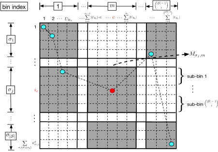
Figure 6: Structure of decoding matrix $\mathbf{M}$, which contains $R$ rows and $C$ columns. Each dashed box represents an element of the matrix $\mathbf{M}$. $\mathbf{M}$ is divided into submatrices $M_{\sigma_{i},m}$ with $\sigma_{i}\in\mathcal{S}\backslash\{\sigma_{k}\}$ and $m\in[\tbinom{|\mathcal{S}|-1}{z}]$. The large grey rectangles are submatrices $M_{\sigma_{i},c}$ with $\sigma_{i}\in\mathcal{H}_{m}$ whose elements are all randomly generated and the large white rectangles are submatrices with $\sigma_{i}\not\in\mathcal{H}_{m}$ whose elements are all zero. The numbers in the boxes are row and column bin indices. The numbers along with the row and column indicate the row index and column index of the matrix respectively. For example, the submatrix $M_{\sigma_{j},m}$ has $\bar{n}_{\sigma_{j},z}^{\mathcal{S}}$ rows and $|\mathcal{V}_{\mathcal{H}_{m}}^{\mathcal{S}\backslash\mathcal{H}_{m}}|$ columns. The right-side numbers are the indices of sub-bins partitioned based on the solution of the feasible conditions: {$\beta_{\sigma_{i},\mathcal{T}}\in\mathbb{Q}^{+}:\sigma_{i}\in\mathcal{T},\sigma_{k}\not\in\mathcal{T},\mathcal{T}\subseteq\mathcal{S},|\mathcal{T}|=z$} and $\beta_{\sigma_{i},\mathcal{T}}=0$ if $\sigma_{i}\not\in\mathcal{T}$. For example, the $\sigma_{j}$-th row bin of the matrix is partitioned into $\binom{|\mathcal{S}|-1}{z}$ sub-bins where the $l$-th part for $l\in[\binom{|\mathcal{S}|-1}{z}]$ contains $\beta_{\sigma_{j},\mathcal{H}_{l}}$ rows. The cyan points (and the red point) in the figure are the elements we choose for the non-zero path $(m_{i_{1},1},m_{i_{2},2},\cdots,m_{i_{C},C}):m_{i_{c},c}\neq 0$ for $c\in[C]$. For example, we can choose the element in the $p$-th row of the $m$-th sub-bin in the $\sigma_{j}$-th row bin for the $c$-th column, where $m$ is the index that $\sum_{i=1}^{m-1}{U}_{\mathcal{H}_{i}}+1\leq c\leq\sum_{i=1}^{m}{U}_{\mathcal{H}_{i}}$, $\sigma_{j}=k_{t}\in\mathcal{H}=\{k_{1},\cdots,k_{z}\}$, which satisfy $\!\!\!\!\!\!\!\sum\limits_{\sigma_{i}\in{\{k_{1},\cdots,k_{t-1}\}}}\!\!\!\!\!\!\!\!\!\!\!\beta_{\sigma_{i},\mathcal{H}_{m}}\!+\!1\leq c\!-\!\sum_{i=1}^{m-1}\!\!{U}_{\mathcal{H}_{i}}\leq\!\!\!\!\!\!\!\!\!\sum\limits_{\sigma_{i}\in{\{k_{1},\cdots,k_{t}\}}}\!\!\!\!\!\!\!\!\beta_{\sigma_{i},\mathcal{H}_{m}}$, and $p=c-\sum_{i=1}^{m-1}|\mathcal{U}_{\mathcal{H}_{j}}^{\mathcal{S}\backslash\mathcal{H}_{j}}|-\!\!\!\!\!\!\sum\limits_{\sigma_{i}\in{\{k_{1},\cdots,k_{t-1}\}}}\!\!\!\!\!\!\!\!\!\!\!\beta_{\sigma_{i},\mathcal{H}_{m}}$, which is the red point in the figure.

Appendix E Correctness of FSCT

For cluster $\mathcal{S}=\{\sigma_{1},\sigma_{2},\cdots,\sigma_{|\mathcal{S}|}\}$, we prove that each receiver $\sigma_{k}$ in the round $z$ can successfully decode its desired IV segments by jointly solving the LCs sent from other nodes in $\mathcal{S}\backslash\{\sigma_{k}\}$.

We index the $\binom{|\mathcal{S}|-1}{z}$ subsets of $\mathcal{S}$ of size $z$ which do not contain Node $\sigma_{k}$ (i.e., $\{\mathcal{T}:\mathcal{T}\subseteq\mathcal{S},|\mathcal{T}|=z,\sigma_{k}\not\in\mathcal{T}\}$) as $\{\mathcal{H}_{1},\cdots,\mathcal{H}_{\binom{|\mathcal{S}|-1}{z}}\}$. Note that FSCT cuts each IV into $|\mathcal{S}|-1$ segments in cluster $\mathcal{S}$. For convenience, we use ${U}_{\mathcal{H}_{i}}$ to denote the number of segments generated from IVs in $\mathcal{V}_{\mathcal{H}_{i}}^{\mathcal{S}\backslash\mathcal{H}_{i}}$. Recall that after receiving the message blocks from other nodes in $\mathcal{S}$, i.e., $\{X_{k,z}^{\mathcal{S}}[{i}]:k\in\mathcal{S}\backslash\{\sigma_{k}\},i\in[\bar{n}_{k,z}^{\mathcal{S}}]\}$, receiver $\sigma_{k}\in\mathcal{S}$ first removes the local segments $\Big{\{}{U}_{\mathcal{T}}^{\mathcal{S}\backslash\mathcal{T}}:\mathcal{T}\subseteq\mathcal{S},|\mathcal{T}|=z,\sigma_{k}\in\mathcal{T}\Big{\}}$ from the messages to generate $R\triangleq\sum_{k\in\mathcal{S}\backslash\{\sigma_{k}\}}\bar{n}_{k,z}^{\mathcal{S}}$ numbers of LCs consisting of $C\triangleq\sum_{i=1}^{\binom{|\mathcal{S}|-1}{z}}{U}_{\mathcal{H}_{i}}$ unknown variables. Let matrix $\mathbf{M}\in\mathbb{R}_{R\times C}$ denote the coefficient matrix of received LCs after removing local segments, which is shown in Fig. 6.

The $R$ rows of the $\mathbf{M}$ will be divided into $|\mathcal{S}|-1$ row bin, with the row bin indices $\sigma_{1},\ldots,\sigma_{k-1},\sigma_{k+1}\ldots,\sigma_{|\mathcal{S}|}$. Each row bin $\sigma_{i}$ contains $n_{\sigma_{i},z}^{\mathcal{S}}$ rows, which represent the number of LCs sent by Node $\sigma_{i}$ in round $z$ of cluster $\mathcal{S}$. Each row bin $\sigma_{i}$, for $i\in\mathcal{S}\backslash\{k\}$, is further partitioned into $\binom{|\mathcal{S}|-1}{z}$ sub-bins, indexed as $\{1,2,\cdots,\binom{|\mathcal{S}|-1}{z}\}$, with the $l$-th sub-bin ($l\in[\tbinom{|\mathcal{S}|-1}{z}]$) containing $\beta_{\sigma_{i},\mathcal{H}_{l}}$ rows, where $\beta_{\sigma_{i},\mathcal{H}_{l}}$ is the non-negative solution of (13): {$\beta_{\sigma_{i},\mathcal{T}}\in\mathbb{Q}^{+}:\sigma_{i}\in\mathcal{T},\sigma_{k}\not\in\mathcal{T},\mathcal{T}\subseteq\mathcal{S},|\mathcal{T}|=z$}, and let $\beta_{\sigma_{i},\mathcal{T}}=0$ if $\sigma_{i}\not\in\mathcal{T}$. Note that from the second constraint $\sum_{\mathcal{T}:\sigma_{i}\in\mathcal{T},\sigma_{k}\not\in\mathcal{T}}\beta_{\sigma_{i},\mathcal{T}}\leq\bar{n}_{\sigma_{i},z}^{\mathcal{S}}$ in (13), we can guarantee that there are enough rows to do partition, and the residual rows after the partition can be brought into the last sub-bin.

The $C$ columns of the $\mathbf{M}$ can be divided into $\binom{|\mathcal{S}|-1}{z}$ column bin, and the $m$-th column bin contains $|U_{\mathcal{H}_{m}}|$ columns which represent the number of segments in $\mathcal{V}_{\mathcal{H}_{m}}^{\mathcal{S}\backslash\mathcal{H}_{m}}$.

Now we split the matrix $\mathbf{M}$ into $\binom{|\mathcal{S}|-1}{z}\times(|\mathcal{S}|-1)$ submatrices $\{M_{\sigma_{i},m}:\sigma_{i}\in\mathcal{S}\backslash\{\sigma_{k}\},m\in[\binom{|\mathcal{S}|-1}{z}]\}$ based on the row and column bins as shown in Fig. 6. Submatrix $M_{\sigma_{i},m}$ has $\bar{n}_{\sigma_{i},z}^{\mathcal{S}}$ rows and $|U_{\mathcal{H}_{m}}|$ columns. If $\sigma_{i}\in\mathcal{H}_{m}$, then the elements of submatrix $M_{\sigma_{i},m}$ are the coefficients of the LCs for sending the segments in $\mathcal{V}_{\mathcal{H}_{m}}^{\mathcal{S}\backslash\mathcal{H}_{m}}$ by Node $\sigma_{i}$ (highlight as the grey rectangles in Fig. 6). If $\sigma_{i}\not\in\mathcal{H}_{m}$, since Node $\sigma_{i}$ did not encode these segments, the elements of $M_{\sigma_{i},m}$ are all zero (highlight as the white rectangles in Fig. 6). Note that the transmission strategy of FSCT guarantees that the feasible condition is satisfied in each round $z$ of cluster $\mathcal{S}$ as stated in Section VI-A1.

Now we need to prove that the linear system is solvable. The main idea is that we first find a non-zero path $(m_{i_{1},1},m_{i_{2},2},\cdots,$ $m_{i_{C},C})$ where $m_{i_{c},c}\neq 0$ for all $c\in[C]$ and $m_{i_{c},c}$ is the element in row $i_{c}$ and column $c$ of $\mathbf{M}$ with all $i_{c}$ different, then select $C$ rows from $\mathbf{M}$ to form a square matrix $(\mathbf{M})^{{}^{\prime}}$ with non-zero diagonal elements, and finally we view the determinant of $(\mathbf{M})^{{}^{\prime}}$ as a non-zero polynomial of $(m_{i_{1},1},m_{i_{2},2},\cdots,m_{i_{C},C})$ [48] so that $(\mathbf{M})^{{}^{\prime}}$ is invertible with high probability by Schwartz-Zippel Lemma [49].

Suppose the column $c\in[C]$ is in the $m$-th column bin. Then, it must satisfy

$$\sum_{i=1}^{m-1}{U}_{\mathcal{H}_{i}}+1\leq c\leq\sum_{i=1}^{m}{U}_{\mathcal{H}_{i}}.$$

For this $m$, we can find $\mathcal{H}_{m}$ and represent its indices as $\mathcal{H}_{m}=\{k_{1},\cdots,k_{z}\}$. Now we choose the row bin

$$\sigma_{j}=k_{t}\in\mathcal{H}_{m}$$ (79a)

such that

$$\sum_{\sigma_{i}\in{\{k_{1},\cdots,k_{t-1}\}}}\!\!\!\!\!\!\!\!\!\!\!\beta_{\sigma_{i},\mathcal{H}_{m}}\!+\!1\leq c\!-\!\sum_{i=1}^{m-1}\!\!{U}_{\mathcal{H}_{i}}\leq\!\!\!\!\!\!\!\!\!\sum_{\sigma_{i}\in{\{k_{1},\cdots,k_{t}\}}}\!\!\!\!\!\!\!\!\beta_{\sigma_{i},\mathcal{H}_{m}}.~{}~{}$$ (79b)

Note that by the first constraint in (13), there always exists such $k_{t}\in\{k_{1},\cdots,k_{z}\}$. Then, we choose the $m$-th sub-bin of the row bin $\sigma_{j}$, which contains $\beta_{\sigma_{j},\mathcal{H}_{m}}$ rows. Finally, we choose the $p$-th row of the $m$-th sub-bin, where

$$p=c-\sum_{i=1}^{m-1}|\mathcal{U}_{\mathcal{H}_{j}}^{\mathcal{S}\backslash\mathcal{H}_{j}}|-\!\!\!\!\!\!\sum_{\sigma_{i}\in{\{k_{1},\cdots,k_{t-1}\}}}\!\!\!\!\!\!\!\!\!\!\!\beta_{\sigma_{i},\mathcal{H}_{m}}$$ (80)

Thus, for each element $m_{i_{c},c},c\in[C]$ in the path, we choose $i_{c}$ as the $p$-th row of the $m$-th sub-bin of the row bin $\sigma_{j}$, i.e.,

$$i_{c}=\sum\limits_{\sigma_{i}\in\{\sigma_{1},\cdots,\sigma_{j}\}}\bar{n}_{\sigma_{i},z}^{\mathcal{S}}+\sum\limits_{i=1}^{m-1}\beta_{\sigma_{j},\mathcal{H}_{i}}+p,$$ (81)

where $m,\sigma_{j},p$ are defined above.

The choice above will lead to a unique row $i_{c}$ for each column $c$, i.e., $i_{a}\neq i_{b}$ if $a\neq b$ for all $a,b\in[C]$. If $i_{a}=i_{b}$, $m,t,p$ in (81) for $i_{a},i_{b}$ will be the same. As $a=b=p+\sum_{i=1}^{m-1}{U}_{\mathcal{H}_{i}}+\!\!\!\!\!\!\!\!\sum\limits_{\sigma_{i}\in{\{k_{1},\cdots,k_{t-1}\}}}\!\!\!\!\!\!\!\!\!\!\!\beta_{\sigma_{i},\mathcal{H}_{m}}$, we can imply that $i_{a}\neq i_{b}$ for $a\neq b$.

Each element $m_{i_{c},c}$ is valid and randomly generated. From (79b) and (80), we have $1\leq p\leq\beta_{\sigma_{j},\mathcal{H}_{m}}$. Hence,

$$i_{c}\geq\sum\limits_{\sigma_{i}\in\{\sigma_{1},\cdots,\sigma_{j}\}}\bar{n}_{\sigma_{i},z}^{\mathcal{S}}+\sum\limits_{i=1}^{m}\beta_{\sigma_{j},\mathcal{H}_{i}}+1,$$ (82)

and

$$i_{c}\leq\sum\limits_{\sigma_{i}\in\{\sigma_{1},\cdots,\sigma_{j}\}}\bar{n}_{\sigma_{i},z}^{\mathcal{S}}+\sum\limits_{i=1}^{m}\beta_{\sigma_{j},\mathcal{H}_{i}}.$$ (83)

Thus, $m_{i_{c},c}$ is in the submatrix $M_{\sigma_{j},m}$ with $\sigma_{j}\in\mathcal{\mathcal{missing}}{H}_{m}$, which implies $m_{i_{c},c}$ is randomly generated for each $c$.

After we find the non-zero path $(m_{i_{1},1},m_{i_{2},2},\cdots,m_{i_{C},C}):m_{i_{c},c}\neq 0$, we select $C$ rows from $\mathbf{M}$ to form a square matrix $(\mathbf{M})^{{}^{\prime}}$ with no non-zero elements along the diagonal:

• The $c$-th row of $(\mathbf{M})^{{}^{\prime}}$ is the $(i_{c})$-th row of $\mathbf{M}$.

• The diagonal elements of $(\mathbf{M})^{{}^{\prime}}$: $m_{c,c}^{{}^{\prime}}=m_{i_{c},c}$ is randomly generated.

View the determinant of $(\mathbf{M})^{{}^{\prime}}$ as a non-zero functions of $(m^{{}^{\prime}}_{1,1},m^{{}^{\prime}}_{2,2},\cdots,m^{{}^{\prime}}_{C,C})$. By the Schwartz-Zippel Lemma, the probability of $(\mathbf{M})^{{}^{\prime}}$ being invertible is high as the field size is sufficiently large.

TABLE VI: List of notations in Appendix E

Notation	Description
$\{\mathcal{H}_{1},\cdots,\mathcal{H}_{\binom{|\mathcal{S}|-1}{z}}\}$	Subsets of $\mathcal{S}$ of size $z$ not containing $\sigma_{k}$, i.e., $\{\mathcal{T}:\mathcal{T}\subseteq\mathcal{S},|\mathcal{T}|=z,\sigma_{k}\not\in\mathcal{T}\}$
${U}_{\mathcal{H}_{i}}$	Number of segments generated from IVs in $\mathcal{V}_{\mathcal{H}_{i}}^{\mathcal{S}\backslash\mathcal{H}_{i}}$, i.e., ${U}_{\mathcal{H}_{i}}=(|\mathcal{S}|-1)\big{|}\mathcal{V}_{\mathcal{H}_{i}}^{\mathcal{S}\backslash\mathcal{H}_{i}}\big{|}$
$R$	Total number of LCs of $(z,\mathcal{S})$-mapped IVs received by Node $\sigma_{k}$ , i.e., $R=\sum_{k\in\mathcal{S}\backslash\{\sigma_{k}\}}\bar{n}_{k,z}^{\mathcal{S}}$
$C$	Number of unknown segments related to $(z,\mathcal{S})$-mapped IVs, i.e., $C=\sum_{i=1}^{\binom{|\mathcal{S}|-1}{z}}{U}_{\mathcal{H}_{i}}$
$\beta_{\sigma_{i},\mathcal{H}_{l}}$ for $\sigma_{i}\in\mathcal{S}\backslash\sigma_{k}$, $l\!\in\![\tbinom{|\mathcal{S}|-1}{z}]$	Non-negative solution of feasible condition (13)
Row bin $\sigma_{i}$ for $\sigma_{i}\in\mathcal{S}\backslash\sigma_{k}$	Row $\sum\limits_{\sigma_{j}\in\mathcal{S}\backslash\sigma_{k},j<i}\bar{n}_{j,z}^{\mathcal{S}}+1$ to Row $\sum\limits_{\sigma_{j}\in\mathcal{S}\backslash\sigma_{k},j\leq i}\bar{n}_{j,z}^{\mathcal{S}}$
Sub-bin $l$ of row bin $\sigma_{i}$ for $i\in[|\mathcal{S}|]\backslash k$, $l\in[\binom{|\mathcal{S}|-1}{z}]$	Row $\sum\limits_{\sigma_{j}\in\mathcal{S}\backslash\sigma_{k},j<i}\!\!\!\!\bar{n}_{j,z}^{\mathcal{S}}\!\!+\!\sum\limits_{n=1}^{l}\beta_{\sigma_{i},\mathcal{H}_{n}}\!\!+\!1$ to Row $\sum\limits_{\sigma_{j}\in\mathcal{S}\backslash\sigma_{k},j<i}\!\!\!\!\bar{n}_{j,z}^{\mathcal{S}}\!\!+\!\sum\limits_{n=1}^{l+1}\beta_{\sigma_{i},\mathcal{H}_{n}}\!\!$
Column bin $m$ for $m\in[\binom{|\mathcal{S}|-1}{z}]$	Column $\sum\limits_{i=1}^{m-1}{U}_{\mathcal{H}_{i}}+1$ to column $\sum\limits_{i=1}^{m}{U}_{\mathcal{H}_{i}}$

References

- [1] J. Dean and S. Ghemawat, “Mapreduce: Simplified data processing on large clusters,” in OSDI’04: Sixth Symposium on Operating System Design and Implementation, (San Francisco, CA), pp. 137–150, 2004.
- [2] M. Zaharia, M. Chowdhury, M. J. Franklin, S. Shenker, and I. Stoica, “Spark: Cluster computing with working sets,” in Proceedings of the 2nd USENIX Conference on Hot Topics in Cloud Computing, HotCloud’10, (USA), p. 10, USENIX Association, 2010.
- [3] F. Ahmad, S. Chakradhar, A. Raghunathan, and T. Vijaykumar, “Tarazu: Optimizing mapreduce on heterogeneous clusters,” International Conference on Architectural Support for Programming Languages and Operating Systems - ASPLOS, vol. 47, 04 2012.
- [4] Z. Zhang, L. Cherkasova, and B. Loo, “Performance modeling of mapreduce jobs in heterogeneous cloud environments,” pp. 839–846, 06 2013.
- [5] S. Li, M. A. Maddah-Ali, Q. Yu, and A. S. Avestimehr, “A fundamental tradeoff between computation and communication in distributed computing,” IEEE Transactions on Information Theory, vol. 64, no. 1, pp. 109–128, 2018.
- [6] J. S. Ng, W. Y. B. Lim, N. C. Luong, Z. Xiong, A. Asheralieva, D. Niyato, C. Leung, and C. Miao, “A comprehensive survey on coded distributed computing: Fundamentals, challenges, and networking applications,” IEEE Communications Surveys Tutorials, vol. 23, no. 3, pp. 1800–1837, 2021.
- [7] G. Yanfei, J. Rao, D. Cheng, and X. Zhou, “ishuffle: Improving hadoop performance with shuffle-on-write,” IEEE Transactions on Parallel and Distributed Systems, vol. 28, pp. 1–1, 01 2016.
- [8] H. Tang, H. Hu, K. Yuan, and Y. Wu, “Communication-efficient coded distributed multi - task learning,” in 2021 IEEE Global Communications Conference (GLOBECOM), pp. 1–6, 2021.
- [9] N. Woolsey, X. Wang, R.-R. Chen, and M. Ji, “Flcd: A flexible low complexity design of coded distributed computing,” IEEE Transactions on Cloud Computing, 2021.
- [10] Y. H. Ezzeldin, M. Karmoose, and C. Fragouli, “Communication vs distributed computation: An alternative trade-off curve,” in 2017 IEEE Information Theory Workshop (ITW), pp. 279–283, 2017.
- [11] E. Parrinello, E. Lampiris, and P. Elia, “Coded distributed computing with node cooperation substantially increases speedup factors,” 02 2018.
- [12] K. Konstantinidis and A. Ramamoorthy, “Leveraging coding techniques for speeding up distributed computing,” in 2018 IEEE Global Communications Conference (GLOBECOM), pp. 1–6, 2018.
- [13] S. Gupta and V. Lalitha, “Locality-aware hybrid coded mapreduce for server-rack architecture,” in 2017 IEEE Information Theory Workshop (ITW), pp. 459–463, 2017.
- [14] K. Konstantinidis and A. Ramamoorthy, “Resolvable designs for speeding up distributed computing,” IEEE/ACM Transactions on Networking, vol. 28, no. 4, pp. 1657–1670, 2020.
- [15] J. Jiang and L. Qu, “Cascaded coded distributed computing schemes based on placement delivery arrays,” IEEE Access, vol. 8, pp. 221385–221395, 2020.
- [16] Q. Yan, X. Tang, and Q. Chen, “Placement delivery array and its applications,” in 2018 IEEE Information Theory Workshop (ITW), pp. 1–5, 2018.
- [17] V. Ramkumar and P. V. Kumar, “Coded mapreduce schemes based on placement delivery array,” in 2019 IEEE International Symposium on Information Theory (ISIT), pp. 3087–3091, 2019.
- [18] A. R. Elkordy, S. Li, M. A. Maddah-Ali, and A. S. Avestimehr, “Compressed coded distributed computing,” IEEE Transactions on Communications, vol. 69, no. 5, pp. 2773–2783, 2021.
- [19] D. Alistarh, D. Grubic, J. Z. Li, R. Tomioka, and M. Vojnovic, “Qsgd: Communication-efficient sgd via gradient quantization and encoding,” in Proceedings of the 31st International Conference on Neural Information Processing Systems, NIPS’17, (Red Hook, NY, USA), p. 1707–1718, Curran Associates Inc., 2017.
- [20] L. Song, C. Fragouli, and T. Zhao, “A pliable index coding approach to data shuffling,” IEEE Transactions on Information Theory, vol. 66, no. 3, pp. 1333–1353, 2020.
- [21] M. Kiamari, C. Wang, and A. S. Avestimehr, “On heterogeneous coded distributed computing,” in GLOBECOM 2017 - 2017 IEEE Global Communications Conference, pp. 1–7, 2017.
- [22] N. Woolsey, R.-R. Chen, and M. Ji, “Coded distributed computing with heterogeneous function assignments,” in ICC 2020 - 2020 IEEE International Conference on Communications (ICC), pp. 1–6, 2020.
- [23] N. Woolsey, R.-R. Chen, and M. Ji, “Cascaded coded distributed computing on heterogeneous networks,” in 2019 IEEE International Symposium on Information Theory (ISIT), pp. 2644–2648, 2019.
- [24] F. Xu, S. Shao, and M. Tao, “New results on the computation-communication tradeoff for heterogeneous coded distributed computing,” IEEE Transactions on Communications, vol. 69, no. 4, pp. 2254–2270, 2021.
- [25] M. A. Maddah-Ali and U. Niesen, “Decentralized coded caching attains order-optimal memory-rate tradeoff,” IEEE/ACM Transactions on Networking, vol. 23, no. 4, pp. 1029–1040, 2015.
- [26] S. Li, Q. Yu, M. A. Maddah-Ali, and A. S. Avestimehr, “A scalable framework for wireless distributed computing,” IEEE/ACM Transactions on Networking, vol. 25, no. 5, pp. 2643–2654, 2017.
- [27] J. Wang, M. Kolar, and N. Srerbo, “Distributed multi-task learning,” in Artificial intelligence and statistics, pp. 751–760, PMLR, 2016.
- [28] M. A. Maddah-Ali and U. Niesen, “Fundamental limits of caching,” IEEE Transactions on Information Theory, vol. 60, no. 5, pp. 2856–2867, 2014.
- [29] U. Niesen and M. A. Maddah-Ali, “Coded caching with nonuniform demands,” IEEE Transactions on Information Theory, vol. 63, no. 2, pp. 1146–1158, 2017.
- [30] J. Hachem, N. Karamchandani, and S. N. Diggavi, “Coded caching for multi-level popularity and access,” IEEE Transactions on Information Theory, vol. 63, no. 5, pp. 3108–3141, 2017.
- [31] J. Zhang, X. Lin, and X. Wang, “Coded caching under arbitrary popularity distributions,” IEEE Transactions on Information Theory, vol. 64, no. 1, pp. 349–366, 2018.
- [32] S. Jin, Y. Cui, H. Liu, and G. Caire, “Structural properties of uncoded placement optimization for coded delivery,” arXiv preprint, 2017. 2201.06300.
- [33] C.-H. Chang, C.-C. Wang, and B. Peleato, “On coded caching for two users with overlapping demand sets,” in ICC 2020 - 2020 IEEE International Conference on Communications (ICC), pp. 1–6, 2020.
- [34] S. Wang and B. Peleato, “Coded caching with heterogeneous user profiles,” in 2019 IEEE International Symposium on Information Theory (ISIT), pp. 2619–2623, 2019.
- [35] C. Zhang, S. Wang, V. Aggarwal, and B. Peleato, “Coded caching with heterogeneous user profiles,” IEEE Transactions on Information Theory, pp. 1–1, 2022.
- [36] A. Sengupta and R. Tandon, “Improved approximation of storage-rate tradeoff for caching with multiple demands,” IEEE Transactions on Communications, vol. 65, no. 5, pp. 1940–1955, 2017.
- [37] M. Ji, A. Tulino, J. Llorca, and G. Caire, “Caching-aided coded multicasting with multiple random requests,” in 2015 IEEE Information Theory Workshop (ITW), pp. 1–5, 2015.
- [38] J. Zhang, X. Lin, and C.-C. Wang, “Closing the gap for coded caching with distinct file sizes,” in 2019 IEEE International Symposium on Information Theory (ISIT), pp. 687–691, 2019.
- [39] A. M. Ibrahim, A. A. Zewail, and A. Yener, “Coded caching for heterogeneous systems: An optimization perspective,” IEEE Transactions on Communications, vol. 67, no. 8, pp. 5321–5335, 2019.
- [40] Q. Wang, Y. Cui, S. Jin, J. Zou, C. Li, and H. Xiong, “Optimization-based decentralized coded caching for files and caches with arbitrary sizes,” IEEE Transactions on Communications, vol. 68, no. 4, pp. 2090–2105, 2020.
- [41] C.-H. Chang and C.-C. Wang, “Coded caching with full heterogeneity: Exact capacity of the two-user/two-file case,” in 2019 IEEE International Symposium on Information Theory (ISIT), pp. 6–10, 2019.
- [42] A. M. Daniel and W. Yu, “Optimization of heterogeneous coded caching,” IEEE Transactions on Information Theory, vol. 66, no. 3, pp. 1893–1919, 2020.
- [43] Q. Yu, S. Li, M. A. Maddah-Ali, and A. S. Avestimehr, “How to optimally allocate resources for coded distributed computing?,” in 2017 IEEE International Conference on Communications (ICC), pp. 1–7, 2017.
- [44] S. Boyd and L. Vandenberghe, Convex Optimization. Cambridge University Press, 2004.
- [45] I. Gohberg and V. Olshevsky, “Fast algorithms with preprocessing for matrix-vector multiplication problems,” Journal of Complexity, vol. 10, 12 1994.
- [46] T. Cormen, C. Leiserson, R. Rivest, and C. Stein, Introduction to Algorithms, Third Edition. 01 2009.
- [47] C. D. Meyer, Matrix Analysis and Applied Linear Algebra. USA: Society for Industrial and Applied Mathematics, 2000.
- [48] M. C. Tsakiris, L. Peng, A. Conca, L. Kneip, Y. Shi, and H. Choi, “An algebraic-geometric approach for linear regression without correspondences,” IEEE Transactions on Information Theory, vol. 66, no. 8, pp. 5130–5144, 2020.
- [49] R. Demillo and R. Lipton, “A probabilistic remark on algebraic program testing.,” Inf. Process. Lett., vol. 7, pp. 193–195, 06 1978.