Finding Approximately Convex Ropes
in the Plane

Abstract

The convex rope problem is to find a counterclockwise or clockwise convex rope starting at the vertex $a$ and ending at the vertex $b$ of a simple polygon $\mathcal{P}$, where $a$ is a vertex of the convex hull of $\mathcal{P}$ and $b$ is visible from infinity. The convex rope mentioned is the shortest path joining $a$ and $b$ that does not enter the interior of $\mathcal{P}$. In this paper, the problem is reconstructed as the one of finding such shortest path in a simple polygon and solved by the method of multiple shooting. We then show that if the collinear condition of the method holds at all shooting points, then these shooting points form the shortest path. Otherwise, the sequence of paths obtained by the update of the method converges to the shortest path. The algorithm is implemented in C++ for numerical experiments.

Keywords: Convex hull; approximate algorithm; convex rope; shortest path; non-convex optimization; geodesic convexity.

MSC2010: MSC 52A30; MSC 52B55; MSC 68Q25; 90C26; MSC 65D18; 68R01.

1 Introduction

Solving automatic grasp planning problems is to evaluate must-touch regions, what forces should be applied to an object, and how those forces can be used by robotic hands [15, 18, 20]. A geometric construction, namely the convex rope posted by Peshkin and Sanderson in 1986 [17] gives valuable information for grasping automatically with robot hands. The problem of finding convex ropes plays a significant role in grasp planning a polygonal object with a simple robot hand. Besides the weight information of the object relevant to grasping and their geometric information are also necessary for this task. To simplify and decrease the number of possible hand configurations, objects are modeled as a set of shape primitives, such as polygons in 2D or polyhedrons, spheres, cylinders, and cones in 3D.

In 2D, determining convex ropes helps to find contact points which are points on a polygonal object corresponding to the robot’s finger joint position (see Fig. 1(i)). For an object in 3D, the automatic grasp planning concentrates on finding must-touch regions on the object to get information about possible hand configurations (see Figs. 1(ii) and (iii)). Contact points usually belong to the trajectory of the convex rope joining two vertices of a simple polygon. These two vertices are not required to be located on the edges of the convex hull of the polygon (see Fig. 2). It turns out to consider that the endpoints of the convex rope can be visible from infinity (see in Sect. 2 for the definition). In the non-convex optimization context, the problem can be stated as follows

$$\min_{(k,x_{0},x_{1},\ldots,x_{k+1})} \sum_{i=0}^{k}\|x_{i}-x_{i+1}\|$$

subject to $$x_{i}\in\mathcal{P},\text{for}\,i=1,2,\ldots,k,\,x_{0}=a,x_{k+1}=b$$

$$]x_{i},x_{i+1}[\cap\hbox{int}(\mathcal{P})=\emptyset,\text{ where }]x,y[:=[x,y]\setminus\{x,y\}.$$

Unfortunately, no optimization methods have been found for solving the problem. In this paper, we consider geometrical methods for solving the problem to get the global solution.

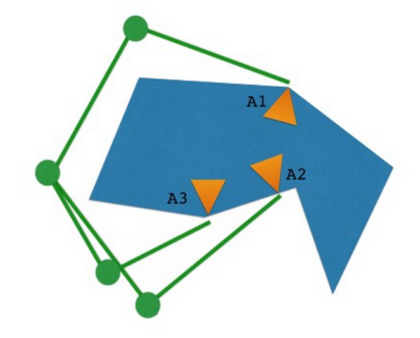
(i)

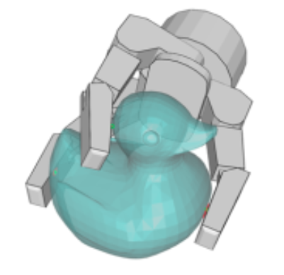
(ii)

(iii)

Figure 1: Illustration of grasping with a simple robot hand; (i): grasping a polygonal object in 2D, images from https://www.shadowrobot.com; (ii) and (iii): grasping a polyhedral object in 3D, images from [18].

Figure 2: Contact points would not necessarily be in edges of the convex hull of the polygon.

The non-convex optimization problem can be addressed via solving alternatively one of two fundamental problems which are convex hull and shortest path problems. In 1986 an algorithm based on evaluating cumulative angles was introduced [17], in which these angles are calculated for each side of the polygon. Another algorithm proposed by An in 2010 [1] was derived from Melkman convex hull algorithm. Using triangulation, a linear time algorithm in 1987 was presented in [8] to compute convex ropes as boundaries of the convex hull of a polyline. In 1990, Heffernan and Mitchell [11] also addressed a linear time algorithm by sorting to a partial triangulation of a polygon. All algorithms mentioned are exact. In 2006, Li and Klette [14] introduced an approximate algorithm that starts with a special trapezoidal segmentation of a polygon and their segmentation is simpler than the triangulation procedure.

In this paper, we present an approximate algorithm using the geometric multiple shooting approach, which was proposed for solving the geometric shortest path problems in 2D and 3D [3, 5, 12]. In particular, the convex rope problem will be formulated into the form of finding shortest paths in a simple polygon since the closed relationship between convex sets and shortest paths. A set is convex if the line segment joining any two points of the set lies completely inside the set. Substituting a line segment joining two points by the shortest path joining these two points expands the notion of classical convexity to geodesic convexity [9, 19]. We then use successfully the method of multiple shooting (MMS for short) to find approximately these shortest paths. The three main factors of the method are given in detail. As an advantage of MMS, instead of solving the problem for the whole formed polygon, we deal with a set of smaller partitioned subpolygons. This is useful in the implementation of devices with limited memory.

In [3], the multiple shooting approach of An et al. is applied to simple polygons with a hypothesis of the so-called “oracle”, not for general simple polygons. The “oracle” condition requests that between two consecutive cutting segments there exists at least one point in which every shortest path joining two corresponding shooting points passes through it, where notions of cutting segments and shooting points are introduced in Sect. 3. Besides, the relationship between the path satisfying the stop condition and the shortest path; the convergence of paths obtained by An et al.’s algorithm is not stated. In the sequence, there are some open questions related to the algorithm in [3] as follows

• Can use MMS for simple polygons that are not ”oracle”?

• If $Z^{*}$ is a path obtained by the algorithm at an iteration which satisfies the stop condition, whether $Z^{*}$ is the shortest path or not?

• Does the sequence of paths $\{Z^{j}\}_{j=0}^{+\infty}$ obtained by the algorithm converges to the shortest path?

In simple polygons, Hai and An in [9] showed the relationship between the convergence of sequences of paths with respect to the Hausdorff distance and the one with respect to the length. In this paper, we will apply this result to get the convergence to the shortest path of the sequence of paths obtained by the proposed algorithm. Particularly, we adapt MMS to the convex rope problem with slight modifications on determining the stop condition and updating new paths to answer these open questions.We construct a simple polygon in which our corresponding algorithm can apply even though the polygon does not satisfy the “oracle” condition (Sect. 3.1). We can also show that, at an iteration step, if a path satisfies the stop condition at all shooting points, then the path and the shortest path are identical. Otherwise, Theorems 1 and 2 state that the sequence of paths obtained by the algorithm converges to the shortest path, then the global solution is obtained.

The rest of the paper is organized as follows. Sect. 2 introduces the convex rope problem and three main factors of MMS. Sect. 3 presents the proposed algorithm in which MMS with three factors (f1)-(f3) can be applied. The correctness of the proposed algorithm and answers for the above open questions is stated by results in Sect. 4. The algorithm is implemented in C++ and numerical results are given and visualized in Sect. 5 to describe how our method works. Some advantages of MMS are established in Sect. 6. Geometrical properties and their proofs are arranged in Appendix.

2 Preliminaries

A vertex of a simple polygon $\mathcal{P}$ is visible from infinity if there exists a ray beginning at the vertex which does not intersect $\mathcal{P}$ anywhere else. In Fig. 3(i), $b$ is visible from infinity with ray $bb^{\prime}$. Clearly, a vertex of the convex hull of $\mathcal{P}$ is also visible from infinity. We say a path starting at the vertex $a$ and ending at the vertex $b$ of $\mathcal{P}$ is counterclockwise (clockwise, resp.) if the interior of $\mathcal{P}$ lies to the left (right, resp.) as we step along the path, starting at $a$.

Definition 1.

The counterclockwise (clockwise, resp.) shortest path starting at $a$ and ending at $b$ of $\mathcal{P}$ that does not enter the interior of $\mathcal{P}$, where $a$ is a vertex of the convex hull of $\mathcal{P}$ and $b$ is visible from infinity, is called a counterclockwise (clockwise, resp.) convex rope starting at $a$ and ending at $b$.

The convex rope problem is necessary to find a counterclockwise (clockwise, resp.) convex rope between $a$ and $b$. For simplicity, we consider the counterclockwise convex rope case only. The clockwise convex rope case is considered similarly. The counterclockwise convex rope between $a$ and $b$ is illustrated as a dashed curve in Fig. 3(i). When both $a$ and $b$ are visible infinity, we obtain another version of the convex rope problem which can be also solved by the same way as the case that $a$ is a vertex of the convex hull of $\mathcal{P}$ by our algorithm. For details see Sect. 3.1.

We now recall some basic concepts and properties. For any points $x,y$ in the plane, we denote $[x,y]:=\{(1-\lambda)x+\lambda y:0\leq\lambda\leq 1\}$, $]x,y]:=[x,y]\setminus\{x\}$, $]x,y[:=[x,y]\setminus\{x,y\}.$ Let $x$ and $y$ be two points in a simple polygon $\mathcal{A}$. The shortest path joining $x$ and $y$ in $\mathcal{A}$, denoted by $\text{SP}(x,y)$, is the path of minimal length joining $x$ and $y$ in $\mathcal{A}$. As shown in [7, 13], $\text{SP}(x,y)$ is a polyline whose vertices except for $x$ and $y$ are reflex vertices of $\mathcal{A}$, i.e., the internal angles at these vertices are at least $\pi$. In addition, these vertices are also reflex vertices of $\text{SP}(x,y)$. Furthermore, let $y^{\prime}\in\mathcal{A}$, for any two line segments $e$ of $\text{SP}(x,y)$ and $g$ of $\text{SP}(x,y^{\prime})$, we have either (i) $e=g$; or (ii) $e$ and $g$ are disjoint or share at most one endpoint. Fundamental concepts such as polylines, polygons, convex (reflex) vertices, shortest paths and their properties which will be used in this paper can be seen in [2, 10] and Appendix.

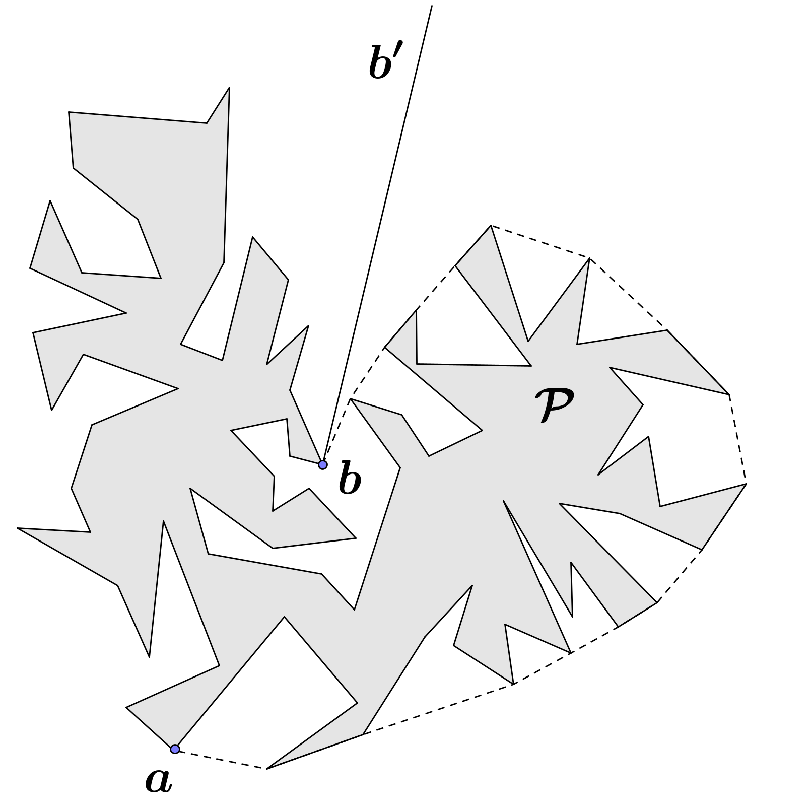
(i)

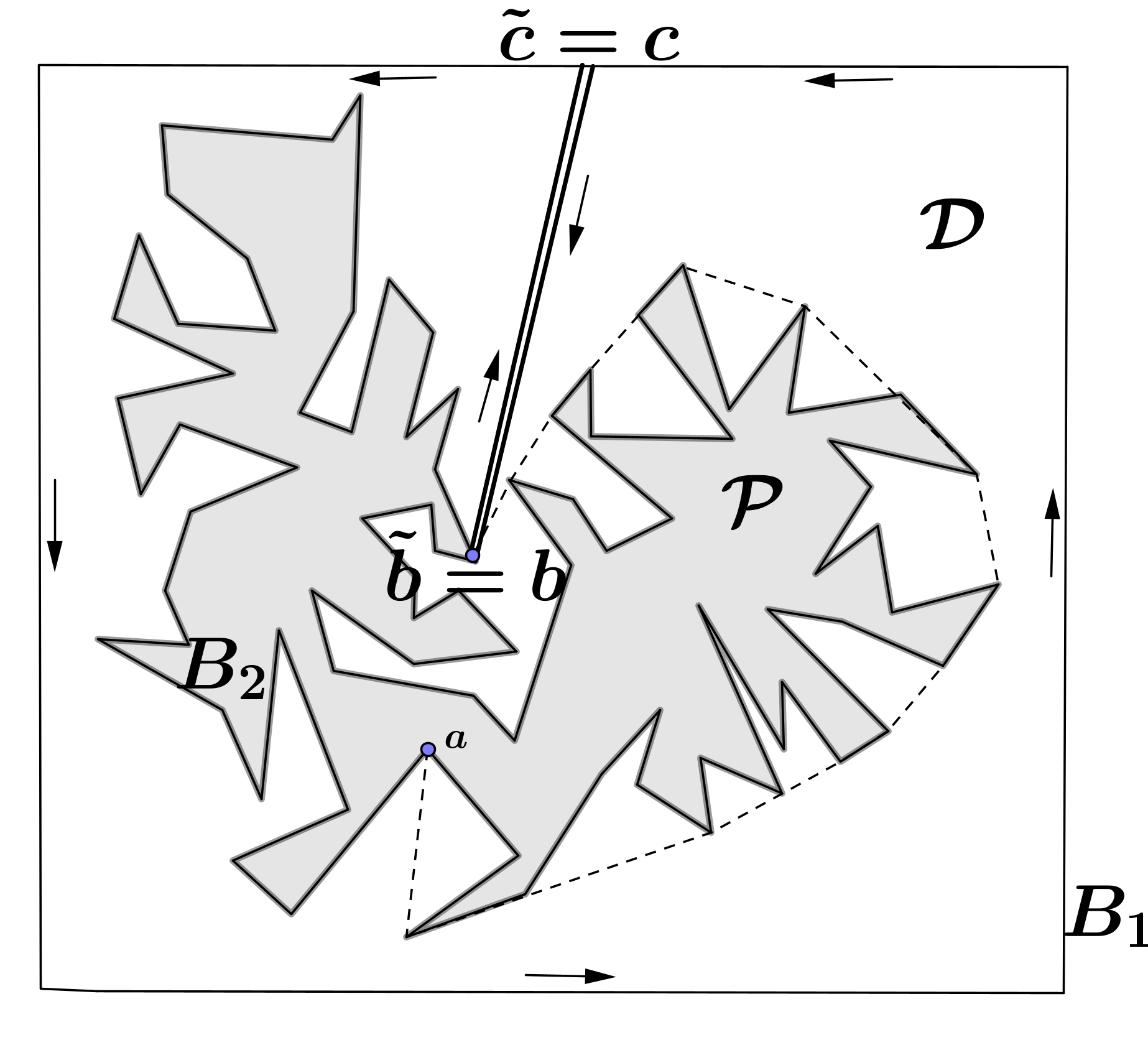
(ii)

Figure 3: The counterclockwise convex rope starting at $a$ and ending at $b$, the case (i): $a$ is a vertex of the convex hull of $\mathcal{P}$ and the case (ii): $a$ is visible from infinity.

Let $x\in\mathbb{R}^{2}$ and $A$ be a nonempty subset of $\mathbb{R}^{2}$, then the distance from $x$ to $A$, denoted by $d(x,A)$, is defined as $d(x,A)=\inf_{y\in A}\|x-y\|,$ where $\|.\|$ is the Euclidean norm in $\mathbb{R}^{2}$. Let $A$ and $B$ be two nonempty subsets of $\mathbb{R}^{2}$. The Hausdorff distance between $A$ and $B$, denoted by $d_{\mathcal{H}}(A,B)$ is defined as $d_{\mathcal{H}}(A,B)=\max\{\sup_{x\in A}d(x,B),\sup_{y\in B}d(y,A)\}$.

Regarding MMS for finding the shortest path joining two points $p$ and $q$ in a domain $\mathcal{D}$ [3, 5, 12], three following factors are included:

• Partition of the domain $\mathcal{D}$ which is a polygon in 2D (polytope in 3D, resp.) into subpolygons (subpolytopes, resp.) is created by cutting segments (cutting slices, resp.). In each cutting segment (the boundary of cutting slice, resp.) we take a point that is called a shooting point;

• Construct a path in $\mathcal{D}$ joining $p$ and $q$, formed by the ordered set of shooting points. A stop condition called collinear condition (straightness condition, resp.) is established at shooting points;

• The algorithm enforces (f2) at all shooting points to check the stop condition. Otherwise, an update of shooting points improves the paths joining $p$ and $q$.

These factors which are established for the convex rope problem are described in the next section.

3 MMS-based Algorithm for Finding Convex Ropes

The proposed algorithm includes two following phases. We first construct a simple polygon such that the convex rope problem is referred to as the problem of finding the shortest path joining two points in the polygon. In the second phase, three factors (f1) - (f3) will be applied for the shortest path problem.

3.1 Constructing a simple polygon $\mathcal{D}$

Take a rectangle $R$ that contains $\mathcal{P}$ and has no edge touching $\mathcal{P}$. Since $b$ is visible from infinity, the ray $bb^{\prime}$ always intersects with $R$ at only one point, say $c$. The line segment $[b,c]$ partitions the non-simple region $R\setminus{\rm int}\mathcal{P}$ into a simple region, similar to that of [19] as follows.

• We insert $[b,c]$ and its copy $[\tilde{b},\tilde{c}]$ into the descriptions of the boundary of $R\setminus{\rm int}\mathcal{P}$. Let $\mathcal{D}$ be a new simple polygon that is determined by a closed polyline including two parts: one part, denoted by $B_{1}$, is a polyline starting at $\tilde{b}$, crossing $\tilde{c}$, going along the boundary of $R$ with the direction of arrows to come $c$ and going to $b$; other, denoted by $B_{2}$, is the polyline starting at $b$ going along the boundary of $\mathcal{P}$ via clockwise order and returning to $\tilde{b}$. Thus $\mathcal{D}$ has the boundary $B_{1}\cup B_{2}$ as shown in Fig. 3(ii).

The non-simple region $R\setminus{\rm int}\mathcal{P}$ is converted into the simple polygon $\mathcal{D}$. By Remark 2 given in Appendix, the convex rope starting at $a$ and ending at $b$ is indeed the shortest path joining $a$ and $b$ in $\mathcal{D}$. Therefore the convex rope problem is deduced to the shortest path problem in $\mathcal{D}$. We can also model the convex rope problem as the shortest path problem in another polygon whose boundary includes the convex hull of $\mathcal{P}$ instead of the rectangle $\mathcal{R}$, see [8]. However computing the convex hull of $\mathcal{P}$ needs linear time whereas the construction of rectangle $\mathcal{R}$ takes constant time when input points are within a given range. According to Remark 2 in Appendix, from now on we focus on finding the shortest path joining $\tilde{b}$ and $b$ in $\mathcal{D}$.

3.2 The factor (f1): partitioning the polygon $\mathcal{D}$

We split the polygon $\mathcal{D}$ into sub-polygons $\mathcal{D}_{i}$ by $N$ cutting segments $\xi_{1},\cdots,\xi_{N}$ ($N\geq 1$) as follows

$$\begin{array}[]{lll}\mbox{+ }\xi_{i}=[u_{i},v_{i}]\subset\mathcal{D}\mbox{ such that }]u_{i},v_{i}[\subset{\rm int}\mathcal{D},\quad u_{i}\in B_{1}\mbox{ and }v_{i}\in B_{2},\,\text{ for }1\leq i\leq N;\\ \mbox{+ }\xi_{i}\mbox{ strictly }\mbox{ separates }\tilde{b}\mbox{ and }b,\text{ for }1\leq i\leq N;\\ \mbox{+ }\xi_{0}=\{\tilde{b}\},\xi_{N+1}=\{b\},[u_{i},v_{i}]\,\cap\,[u_{j},v_{j}]=\emptyset,\text{ for }i\neq j,\,1\leq i,j\leq N;\\ \mbox{+ }\mathcal{D}_{i}\mbox{ is bounded by }B_{1},B_{2},\mbox{ cut segments }\xi_{i}\mbox{ and }\xi_{i+1},\text{ for }0\leq i\leq N;\\ \mbox{+ }\mbox{int}\mathcal{D}_{i}\cap\mbox{int}\mathcal{D}_{j}=\emptyset,\mbox{ for }i\neq j,\,0\leq i,j\leq N\mbox{ and }\mathcal{D}=\bigcup_{i=0}^{N}\mathcal{D}_{i}.\end{array}$$ (1)

A partition given by (1) is illustrated in Fig. 4(i). In the first step, we take a point in each cutting segment. Two consecutive initial points are connected by the shortest path in the corresponding sub-polygon. The initial path is received by combining these shortest paths. For convenience, these initial points are chosen at endpoints $v_{i}$ of $\xi_{i}$. For each iteration step, which is discussed carefully in next sections (3.3 and 3.4), we obtain an ordered set of points $\{a_{i}|\,a_{i}\in\xi_{i},i=1,2,\ldots,N\}$ and a path $\gamma=\cup_{i=0}^{N}\text{SP}(a_{i},a_{i+1})$, where $\text{SP}(a_{i},a_{i+1})$ is the shortest path joining $a_{i}$ and $a_{i+1}$ in $\mathcal{D}_{i}$ and $a_{0}=\tilde{b},a_{N+1}=b$. Such a point $a_{i}$ is called a shooting point and $\gamma$ is called the path formed by the set of shooting points (see [2]).

It is clear that the shortest path joining $a_{i},a_{i+1}$ in $\mathcal{D}_{i}$ and that in $\mathcal{D}$ are identical. However, in the implementation, finding the shortest paths in these sub-polygons makes more efficient use of time and memory than that in an entire polygon. Here $\text{SP}(a_{i},a_{i+1})$ could be computed by any known algorithm for finding the shortest paths in simple polygons. Throughout this paper, when we say $\text{SP}(x,y)$ without further explanation, it means the shortest path joining $x$ and $y$ in the connected union of sub-polygons containing $x$ and $y$ of $\mathcal{D}$.

3.3 The factor (f2): establishing and checking the collinear condition

Firstly, we present a so-called collinear condition inspired by Corollary 4.3 in [10]. Recall that $a_{i}\in[u_{i},v_{i}]$, for all $i=1,2,\ldots,N$, where $a_{0}=\tilde{b},a_{N+1}=b$. The upper angle created by $\text{SP}(a_{i-1},a_{i})$ and $\text{SP}(a_{i},a_{i+1})$ with respect to $[u_{i},v_{i}]$, denoted by $\angle\left(\text{SP}(a_{i-1},a_{i}),\text{SP}(a_{i},a_{i+1})\right)$, is defined to be the angle of the polyline $\text{SP}(a_{i-1},a_{i})\cup\text{SP}(a_{i},a_{i+1})$ at $a_{i}$ containing the ray $a_{i}u_{i}$. For each $i=1,2,\ldots,N$, the collinear condition states that:

• If $a_{i}\in]u_{i},v_{i}[$, we say that $a_{i}$ satisfies the collinear condition when the upper angle created by $\text{SP}(a_{i-1},a_{i})$ and $\text{SP}(a_{i},a_{i+1})$ is equal to $\pi$ (i.e, $\angle\left(\text{SP}(a_{i-1},a_{i}),\text{SP}(a_{i},a_{i+1})\right)=\pi$).
  If $a_{i}=v_{i}$, we say that $a_{i}$ satisfies the collinear condition when the upper angle created by $\text{SP}(a_{i-1},a_{i})$ and $\text{SP}(a_{i},a_{i+1})$ is at least $\pi$ (i.e, $\angle\left(\text{SP}(a_{i-1},a_{i}),\text{SP}(a_{i},a_{i+1})\right)\geq\pi$).

Let $\gamma^{*}$ be the shortest path joining $\tilde{b}$ and $b$ in $\mathcal{D}$, i.e., $\gamma^{*}={\rm SP}(\tilde{b},b).$ According to Remark 2 in Appendix, Collinear Condition (B) does not include the case $a_{i}=u_{i}$.

3.4 The factor (f3): updating shooting points

Suppose that in $j^{th}$-iteration step, we have a set of shooting points $\{a_{i}\}_{i=1}^{N}$ and $\gamma=\cup_{i=0}^{N}\text{SP}(a_{i},a_{i+1})$ is the path formed by the set of shooting points, where $a_{0}=\tilde{b},a_{N+1}=b$. If Collinear Condition (B) holds at all shooting points, by Proposition 1 in Sect. 4, the path obtained by the algorithm is the shortest, and our algorithm stops. Otherwise, we update shooting points to get a path formed by the set of new shooting points in which the sequence of paths obtained converges to the shortest path, according to Theorems 1 and 2. Assuming that Collinear Condition (B) does not hold at all shooting points, we update shooting points as follows

• For $i=1,2\ldots,N$, fix $t_{i-1}\in\text{SP}(a_{i-1},a_{i}),t_{i}\in\text{SP}(a_{i},a_{i+1})$ such that $t_{i-1},t_{i}$ are not identical to shooting points. We call such point $t_{i-1}$ ($t_{i}$, resp.) the temporary point with respect to $a_{i-1}$ ($a_{i}$, resp.). Let $a^{next}_{i}=\text{SP}(t_{i-1},t_{i})\cap[u_{i},v_{i}]$.

  The intersection point $a^{next}_{i}$ exists uniquely since $[u_{i},v_{i}]$ divides $\mathcal{D}$ into two parts, one that contains $t_{i-1}$ and one that contains $t_{i}$. We update shooting point $a_{i}$ to $a^{next}_{i}$ (see Fig. 4(iii)).

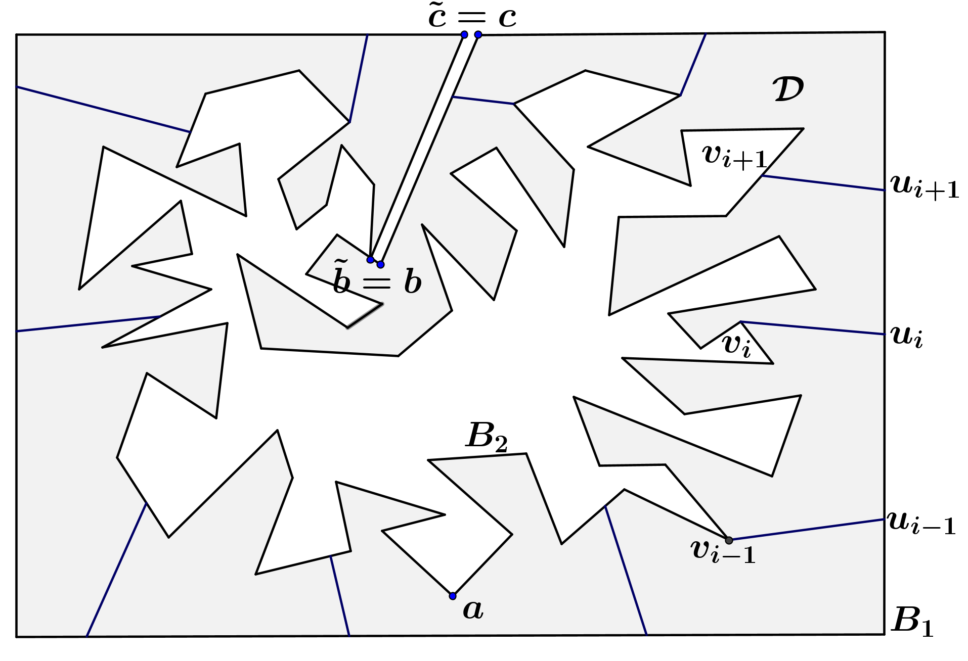
(i)

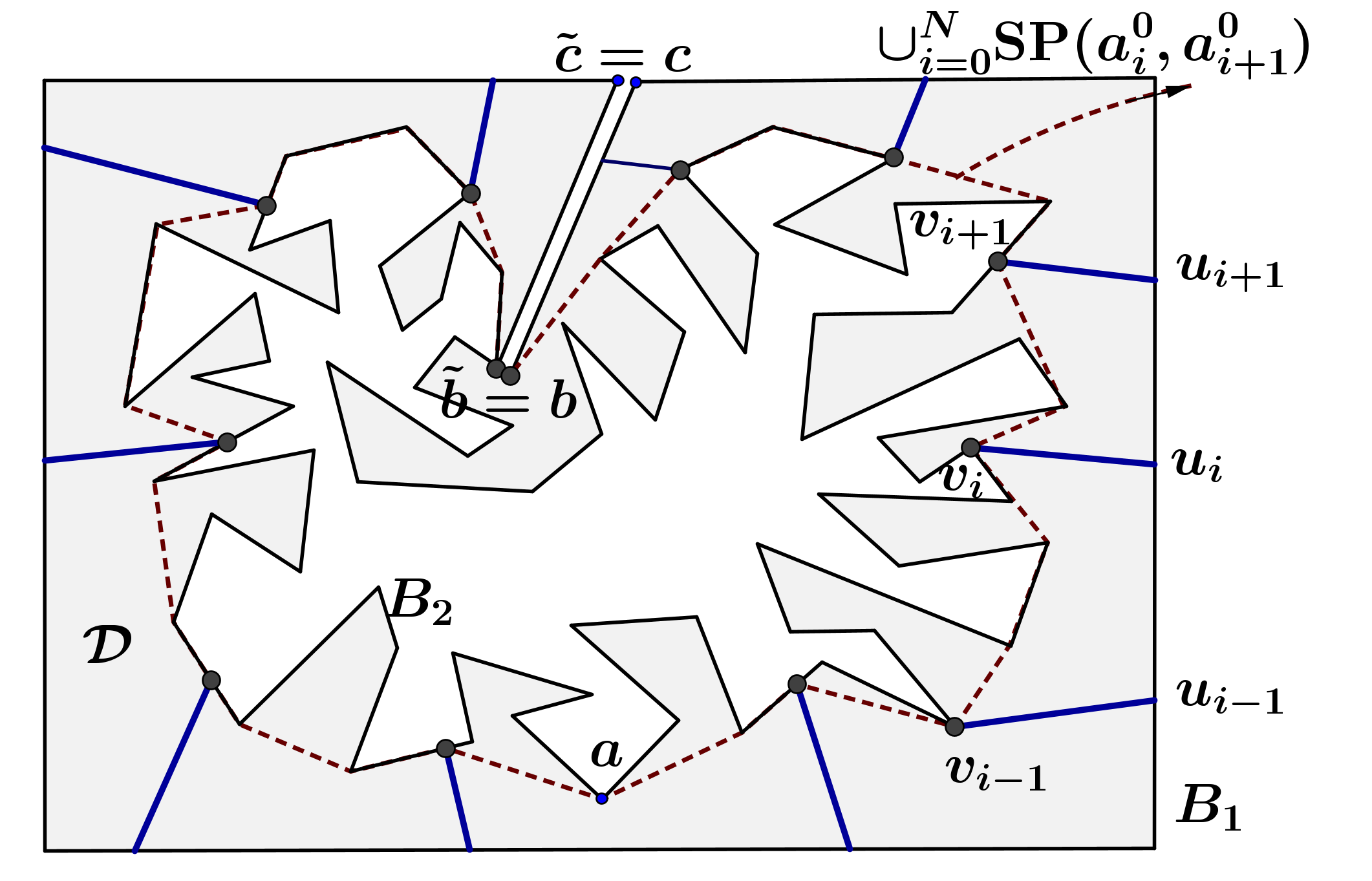
(ii)

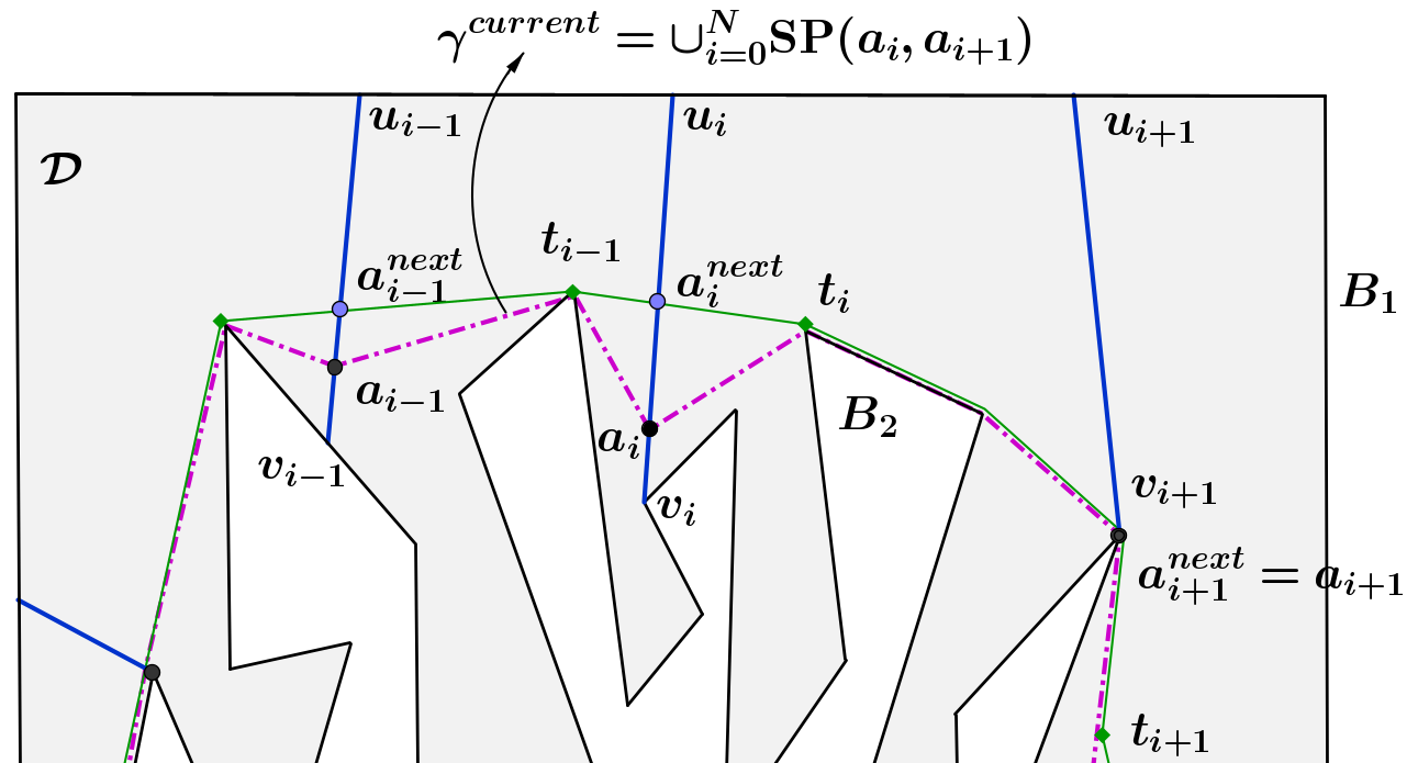
(iii)

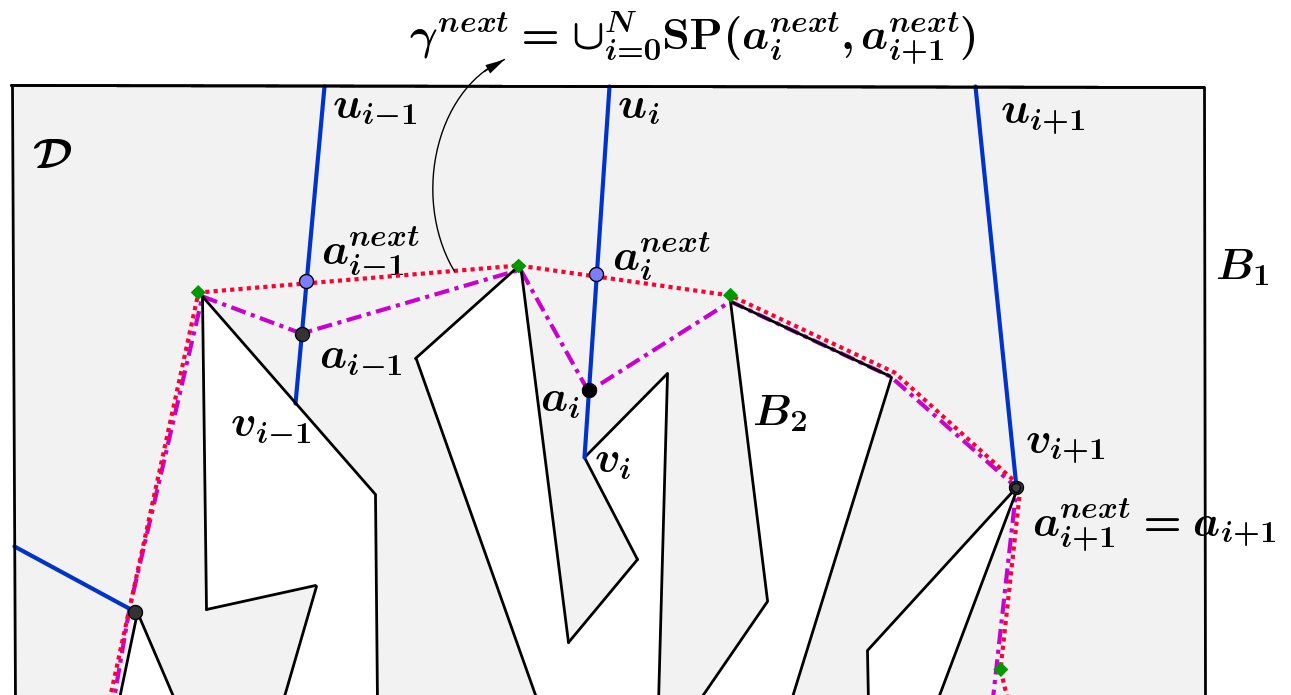
(iv)

Figure 4: (i): Illustration of partitioning $\mathcal{D}$; (ii): the set of initial shooting points consisting of $\tilde{b}$, $v_{i},(i=1,2,\ldots,N)$ and $b$. (black big dots) and the path formed by the set (dashed polyline); (iii): illustration of taking temporary points and finding $a_{i}^{next}=\text{SP}(t_{i-1},t_{i})\cap\xi_{i}$; (iv): the update $\gamma^{current}$ (dashed polyline) to $\gamma^{next}$ (solid polyline).

In particular, if $\text{SP}(a_{i},a_{i+1})$ is a line segment, we choose $t_{i}$ as the midpoint of $\text{SP}(a_{i},a_{i+1})$. Otherwise, $t_{i}$ is chosen as an endpoint of $\text{SP}(a_{i},a_{i+1})$ that is not identical to $a_{i}$ and $a_{i+1}$. We can update shooting points in which the collinear condition does not hold and keep the remaining shooting points. But the proposed algorithm will update all shooting points. Because if $a_{i}$ satisfies Collinear Condition (B), then the update gives $a_{i}^{next}=a_{i}$ due to Proposition 2 (in Sect. 4).

3.5 The Proposed Algorithm

1:A simple polygon $\mathcal{P}$, $b\in\mathcal{P}$ and its copy $\tilde{b}$, an integer number $N\geq 1$.

2:An approximate convex rope starting at $\tilde{b}$ and ending at $b$.

3:Construct a simple polygon $\mathcal{D}$ with the boundary $B_{1}\cup B_{2}$ as shown in (A). $\triangleright$ see Fig. 3(ii)

4:Divide $\mathcal{D}$ into $\mathcal{D}_{i}$ satisfying (1) by cutting segments $[u_{i},v_{i}]$, where $u_{i}\in B_{1},v_{i}\in B_{2}$ ($i=1,\ldots,N$) $\triangleright$ see Fig. 4(i)

5:Take an ordered set $\{a_{i}\}_{i=0}^{N+1}$ initial shooting points consisting of $\tilde{b}$, $v_{i},(i=1,2,\ldots,N)$ and $b$. Let $\gamma^{current}$ be the path formed by $\{a_{i}\}_{i=0}^{N+1}$. $\triangleright$ see Fig. 4(ii)

6:$flag\leftarrow true$, $a_{i}^{next}\leftarrow a_{i}$ and $\gamma^{next}$ is the path formed by $\{a_{i}^{next}\}_{i=0}^{N+1}$.

7:Call Procedure Collinear_Update($\gamma^{current},\gamma^{next},flag$) $\triangleright$ see Figs. 4(iii) and (iv)

8:If Collinear Condition(B) holds at all shooting points, i.e., $flag=true$, stop and return $\gamma^{next}$. $\triangleright$ the shortest path is obtained by Proposition 1

9:Otherwise, i.e, $flag=false$, then $\gamma^{current}\leftarrow\gamma^{next}$ and go to step 7.

10:return $\gamma^{next}$.

For each iteration step, we need to check Collinear Condition (B) and update shooting points given by (C) to get a better path. Then Procedure Collinear_Update($\gamma^{current},\gamma^{next},flag$) of the proposed algorithm performs checking condition (B) and updating the shooting point $a_{i}$ to $a_{i}^{next}$.

1:procedure Collinear_Update($\gamma^{current},\gamma^{next},flag$)

2:    $flag\leftarrow true$

3:    for $i=0,1,\ldots,N$ do

4:          Take temporary points $t_{i}$ on $\text{SP}(a_{i},a_{i+1})$ such that  if $\text{SP}(a_{i},a_{i+1})$ is a line segment, $t_{i}$ is the midpoint of $\text{SP}(a_{i},a_{i+1})$,  for if not, $t_{i}$ is an endpoint of $\text{SP}(a_{i},a_{i+1})$ that is not identical to $a_{i}$ and $a_{i+1}$.

5:         if  $a_{i}\in]u_{i},v_{i}[$ then

6:             if $\angle\left(\text{SP}(a_{i-1},a_{i}),\text{SP}(a_{i},a_{i+1})\right)=\pi$ then $\triangleright$ Collinear Condition (B) is checked

7:                 Set $a_{i}^{next}\leftarrow a_{i}$

8:             else call $\text{SP}(t_{i-1},t_{i})$

9:                 Set $a_{i}^{next}$ be the intersection point of $\text{SP}(t_{i-1},t_{i})$ and $[u_{i},v_{i}]$ $\triangleright$ due to (C)

10:                 $flag\leftarrow false$              

11:         else $\triangleright$ $a_{i}=v_{i}$

12:             if $\angle\left(\text{SP}(a_{i-1},a_{i}),\text{SP}(a_{i},a_{i+1})\right)\geq\pi$ then $\triangleright$ Collinear Condition (B) is checked

13:                 Set $a_{i}^{next}\leftarrow a_{i}$

14:             else call $\text{SP}(t_{i-1},t_{i})$

15:                 Set $a_{i}^{next}$ the intersection point of $\text{SP}(t_{i-1},t_{i})$ and $[u_{i},v_{i}]$ $\triangleright$ due to (C)

16:                 $flag\leftarrow false$                           

17:    $a_{0}^{next}=\tilde{b},a_{N+1}^{next}=b$

4 The Correctness of the Proposed Algorithm

The following proposition shows that the path satisfying Collinear Condition (B) is the shortest path $\gamma^{*}$ joining $\tilde{b}$ and $b$.

Proposition 1.

Let $\gamma^{current}$ be a path formed by a set of shooting points, which joins $\tilde{b}$ and $b$ in $\mathcal{D}$. If Collinear Condition (B) holds at all shooting points, then $\gamma^{current}=\gamma^{*}.$

Proposition 2.

Collinear Condition (B) holds at $a_{i}$ if and only if ${\rm SP}(t_{i-1},t_{i})\cap[u_{i},v_{i}]=a_{i}$, where $t_{i-1}$ and $t_{i}$ are temporary points w.r.t. $a_{i-1}$ and $a_{i}$.

Theorem 1.

The algorithm is convergent. It means that if the algorithm stops after a finite number of iteration steps (i.e., Collinear Condition (B) holds at all shooting points), we obtain the shortest path, otherwise, the sequence of paths $\{\gamma^{j}\}$ converges to $\gamma^{*}$ in Hausdorff distance (i..e., $d_{\mathcal{H}}(\gamma^{j},\gamma^{*})\rightarrow 0$ as $j\rightarrow\infty$, where $\gamma^{j}$ be a path obtained by the algorithm in $j^{th}$-iteration step).

Since the function of the length of paths is lower semi-continuous but not continuous, the event $d_{\mathcal{H}}(\gamma^{j},\gamma^{*})\rightarrow 0$ as $j\rightarrow\infty$ does not ensure the convergence of the sequence of lengths of these paths. However, this holds for the sequence of paths obtained by the proposed algorithm. This is shown in the below theorem.

Theorem 2.

The sequence of lengths of paths obtained by the proposed algorithm has the following properties:

• The sequence is decreasing, i.e., Procedure Collinear_Update($\gamma^{current},\gamma^{next},flag$) gives $l\left(\gamma^{next}\right)\leq l\left(\gamma^{current}\right)$. If Collinear Condition (B) does not hold at some shooting point, then the inequality above is strict.

• The sequence converges to $l(\gamma^{*})$.

Theorem 3.

Given a fixed number $N$ of cutting segments, the proposed algorithm runs in $O(kn)$ time, where $n$ is the number of vertices of $\mathcal{P}$, $k$ is the number of iterations to get the required path joining $\tilde{b}$ and $b$.

The proofs of the above propositions and theorems are given in Appendix.

5 Numerical Experiments

In the implementation, assume that the boundary of $\mathcal{P}$ consists of two polylines with integer coordinates that are monotone w.r.t. $x$-coordinate axis, and the cutting segments $\xi_{i}$ are parallel to $y$-coordinate axis. The monotone condition appears because we use a procedure for finding the shortest path joining two consecutive shooting points inside sub-polygons $\mathcal{D}_{i}$ as shown in [4]. The algorithm is implemented in C++ programming language. The codes are compiled and executed by GNU Compiler Collection under platform Ubuntu Linux 18.04, Processor 2.50GHz Core i5.

To check whether Collinear Condition (B) holds or not at a shooting point $a_{i}$, we calculate the upper angle at $a_{i}$ or determine if $a_{i}^{next}$ coincides with $a_{i}$ or not. Two ways are the same by Proposition 2. Here we use the latter way. We need a tolerance, say $\epsilon$, to check for the coincidence of points when implementing. Collinear Condition (B) holds at $a_{i}$ if $\|a_{i}^{next}-a_{i}\|<\epsilon$, for all $1\leq i\leq N$. Moreover, by Lemma 4 in Appendix, the condition $\|a_{i}^{next}-a_{i}\|<\epsilon$, $1\leq i\leq N$ also applies to determine $\{\gamma^{j}\}$ converging to $\gamma^{*}$. The actual runtime of our algorithm grows with the decreasing of $\epsilon$. This effect is given in Table 1 and Fig 8, where $\epsilon$ changes from $10^{0}$ to $10^{-9}$, and the problem is to find an approximate convex rope starting at the copy $\tilde{b}$ of a fixed point $b$ and ends at $b$ of the polygon having 3000 vertices and 200 cutting segments. Figs. 5, 6, and 7 show the results when $\epsilon=10^{6}$ and the number of vertices of $\mathcal{P}$ is $100$, $400$, and $800$, respectively. Herein, the convex ropes start at $a$ and end at $b$, where $a$ is a visible infinity point that plays the same role as $b$ ($a=\tilde{b}$) or a vertex of the convex hull of $\mathcal{P}$.

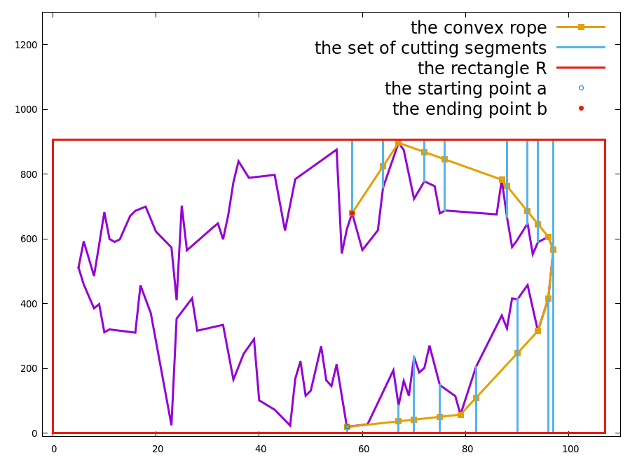
(i)

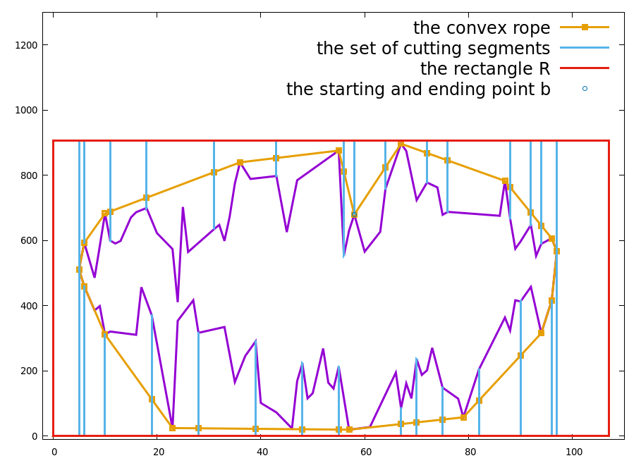
(ii)

Figure 5: Convex ropes of a polygon with 200 vertices: (i) the convex rope starting at a vertex of the convex hull of $\mathcal{P}$ and ending at a point that is visible from infinity; (ii) the convex rope starting and ending at the same point that is visible from infinity.

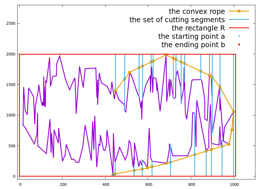
(i)

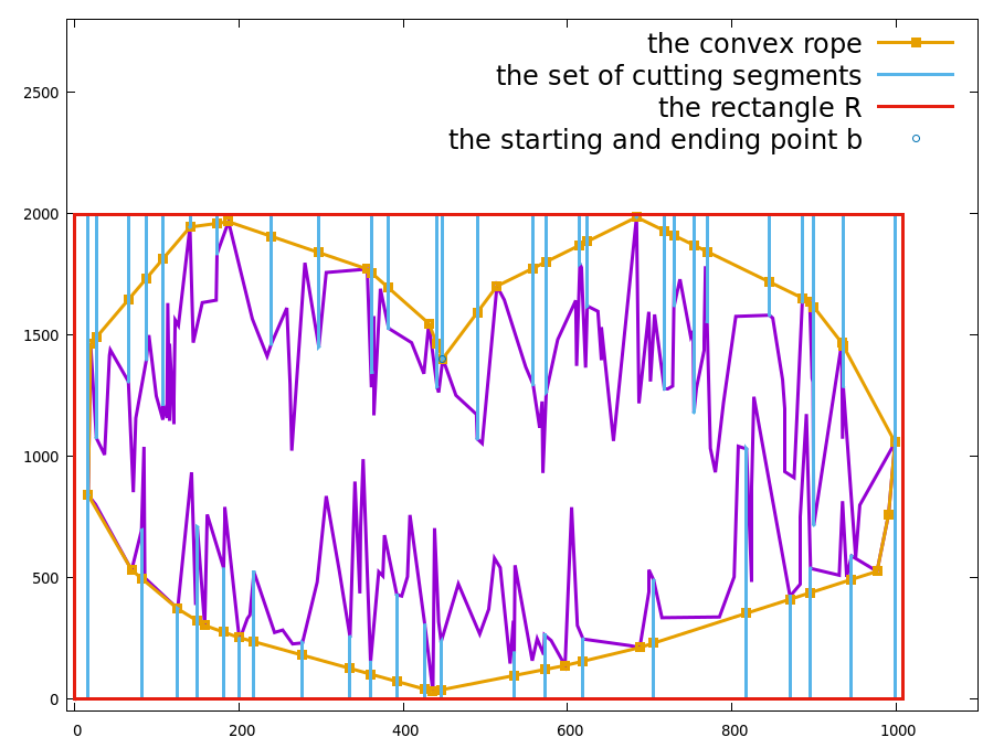
(ii)

Figure 6: Convex ropes of a polygon with 400 vertices: (i) the convex rope starting at a vertex of the convex hull of $\mathcal{P}$ and ending at a point that is visible from infinity; (ii) the convex rope starting and ending at the same point that is visible from infinity.

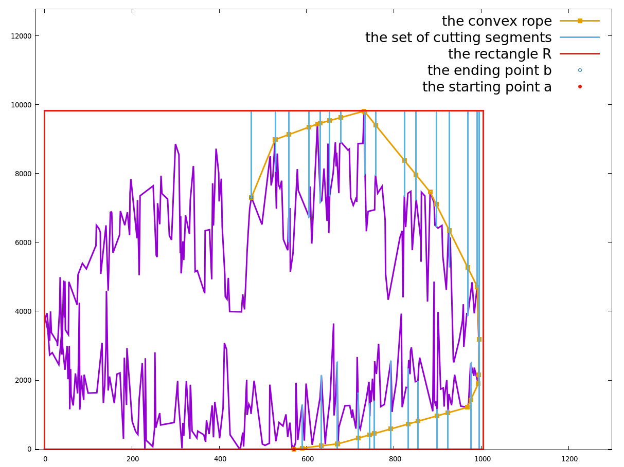
(i)

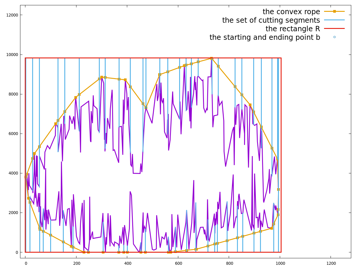
(ii)

Figure 7: Convex ropes of a polygon with 800 vertices: (i) the convex rope starting at a vertex of the convex hull of $\mathcal{P}$ and ending at a point that is visible from infinity; (ii) the convex rope starting and ending at the same point that is visible from infinity.

6 Conclusion

We presented the use of MMS with three factors (f1)-(f3) for approximately solving the convex rope problem. Although the “oracle” condition does not hold for polygon $\mathcal{D}$ as in [3], we dealt with three open questions presented in Sect. 1. We proved that the shortest path is well determined if the collinear condition holds at all shooting points. Otherwise, the sequence of paths obtained from new shooting points by the update of the method converges in Hausdorff distance to the shortest path. The proposed algorithm was implemented in C++ and some numerical examples were given to show that the method is suitable for the problem. On the other side, as an advantage of MMS by the factor (f1) [6], instead of solving the problem for the whole formed polygon, we deal with a set of smaller partitioned subpolygons. Consequently, the memory consuming of the algorithm should be low. This is useful when considering to deploy the method in robotic applications with limited computing resources. This will be a further research in the future.

Table 1: The actual runtime of the proposed algorithm and the length of corresponding convex ropes when $\epsilon$ changes, where the convex ropes of a polygon having 3000 vertices start and end at the same point that is visible from infinity.

Tolerance $\epsilon$	The runtime (secs)	Length of paths
$10^{0}$	$14.26$	$432322.554$
$10^{-1}$	$44.33$	$432312.019$
$10^{-2}$	$106.96$	$432311.361$
$10^{-3}$	$257.45$	$432311.340$
$10^{-4}$	$398.17$	$432311.339$
$10^{-5}$	$553.05$	$432311.339$
$10^{-6}$	$693.02$	$432311.339$
$10^{-7}$	$881.29$	$432311.339$
$10^{-8}$	$1053.78$	$432311.339$
$10^{-9}$	$1217.04$	$432311.339$

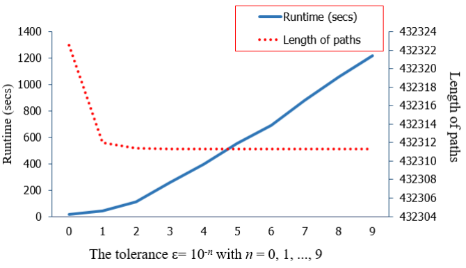
Figure 8: The dependence of the runtime of the proposed algorithm and the length of corresponding convex ropes on $\epsilon$, where the convex ropes of a polygon having 3000 vertices starting and ending at the same point that is visible from infinity.

Appendix

A Shortest paths and convex ropes

With the construction of $\mathcal{D}$ as shown by (A) in Sect. 3.1, vertices of $\mathcal{D}$ on $B_{1}$ except for $b$ and $\tilde{b}$ are convex (see Fig. 3(ii)). We have the following

Remark 1.

The shortest path joining $a$ and $b$ in $\mathcal{D}$ does not depend on the rectangle $R$, i.e, we can replace $R$ with any rectangle that contains $\mathcal{P}$ and has no edge touching $\mathcal{P}$ to obtain another polygon $\mathcal{D}^{\prime}$ in which shortest paths joining $a$ and $b$ in $\mathcal{D}$ and $\mathcal{D}^{\prime}$ are the same. Furthermore, $\text{SP}(a,b)$ never touches $B_{1}$ of $\mathcal{D}$ except for $b$.

Remark 2.

The convex rope starting at $a$ and ending at $b$ of $\mathcal{P}$ can be obtained by solving directly the problem of finding the shortest path joining $a$ and $b$ inside $\mathcal{D}$. If $a$ is a vertex of the convex hull of $\mathcal{P}$, then the shortest path contains $a$ and never touches the boundary $B_{1}$ of $\mathcal{D}$ except for $\tilde{b}$ and $b$. More generally, if $a$ is visible from infinity, then $\tilde{b}$ plays the same role as $a$ (see Fig. 3(ii)). Therefore from now on, we only focus on finding the shortest path joining $\tilde{b}$ and $b$ in $\mathcal{D}$.

B The proofs of propositions and theorems given in Sect. 4

Lemma 1 is presented without a proof (since the proof is similar to that of Proposition 2.19, [2]).

Lemma 1.

Suppose that $\gamma$ is the shortest path joining two given points $p$ and $q$ in a polygon $\mathcal{A}$ such that $\gamma$ intersects a cutting segment $[u,v]$ at a point, say $a$. If $a\in]u,v[$, then $\angle\left(\gamma(p,a),\gamma(a,q)\right)=\pi$.

The proof of Proposition 1:

Proof.

Let $\gamma^{current}=\cup_{i=0}^{N}\text{SP}(a_{i},a_{i+1})$ where $\{a_{i}\}_{i=1}^{N}$ is a set of shooting points and $a_{0}=\tilde{b},a_{N+1}=b$. Assume the contrary that $\gamma^{current}$ and $\gamma^{*}$ are distinct. There are two distinct points $u,v$ which are common points to both $\gamma^{current}$ and $\gamma^{*}$ such that $\gamma^{current}(u,v)\cap\text{SP}(u,v)=\{u,v\}$, where $\gamma^{current}(u,v)$ is the sub-path of $\gamma^{current}$ from $u$ to $v$. Note that $\text{SP}(u,v)$ is also a sub-path of $\gamma^{*}$. Two points $u$ and $v$ always exist and may be identical to $\tilde{b}$ and $b$, respectively. Then $\gamma^{current}(u,v)$ and $\text{SP}(u,v)$ form a simple polygon with $m$ vertices $p_{1}=u,p_{2},\ldots,p_{k}=v,p_{k+1}\ldots,p_{m}$ (see Fig. 9(i)). Let $\alpha_{j}$ be the internal angle at $p_{j}$, with $j=1,2,\ldots,m$. By the properties of shortest paths, if $p_{j}\in\text{SP}(u,v)$ then vertices of $\text{SP}(u,v)$ except for $u$ and $v$ are reflex vertices of $\text{SP}(u,v)$, i.e., $\alpha_{j}>\pi$. If $p_{j}\in\gamma^{current}(u,v)$, then $p_{j}$ is either a shooting point or a reflex vertex of $\text{SP}(a_{i},a_{i+1})$ with some index $i\in\{1,2,\ldots,N\}$. If $p_{j}$ is a shooting point, then $\alpha_{j}\geq\pi$ since Collinear Condition (B) holds at all shooting points. The equality does not occur, because $p_{j}$ is a vertex of $\gamma^{current}$, and thus $\alpha_{j}>\pi$. If $p_{j}$ is a reflex vertex of $\text{SP}(a_{i},a_{i+1})$ with some index $i\in\{1,2,\ldots,N\}$, we also get $\alpha_{j}>\pi$. Hence $\alpha_{j}>\pi$ for $j\in\{1,2,\ldots,m\}\setminus\{1,k\}$. Since the sum of the measures of the internal angles of the simple polygon with $m$ vertices is $(m-2)\pi$, we have $(m-2)\pi=\sum_{j=1}^{m}\alpha_{i}>\alpha_{1}+(m-2)\pi+\alpha_{k}>(m-2)\pi.$ The contradiction deduces $\gamma^{current}=\gamma^{*}$. ∎

The proof of Proposition 2:

Proof.

$(\Rightarrow)$ Assuming that Collinear Condition (B) holds at $a_{i}$, to show that $\text{SP}(t_{i-1},t_{i})\cap[u_{i},v_{i}]=a_{i}$, we just need to prove that $\text{SP}(t_{i-1},t_{i})=\text{SP}(t_{i-1},a_{i})\cup\text{SP}(a_{i},t_{i})$ Assume the contrary, we use the same way of the proof of Proposition 1 and the property that the sum of the internal angles in a simple polygon with $m$ vertices is $(m-2)\pi$ to obtain a contradiction.

$(\Leftarrow)$ Assume that $\text{SP}(t_{i-1},t_{i})\cap[u_{i},v_{i}]=a_{i}$. Therefore $a_{i}$ belongs to $\text{SP}(t_{i-1},t_{i})$. If $a_{i}=v_{i}$, then $\angle\left(\text{SP}(t_{i-1},a_{i}^{next}),\text{SP}(a_{i}^{next},t_{i})\right)\geq\pi$ by the property of shortest paths. If $a_{i}\in]u_{i},v_{i}[$, then $\angle\left(\text{SP}(t_{i-1},a_{i}^{next}),\text{SP}(a_{i}^{next},t_{i})\right)=\pi$ due to Lemma 1. Thus Collinear Condition (B) holds at $a_{i}$. ∎

To prove Theorems 1, and 2 we need Proposition 3, Proposition 4 and Corollary 1. Next, assuming that a partition of $\mathcal{D}$ is given by (1), we have

Proposition 3.

We have $\gamma^{*}\subset\cup_{i=0}^{N}\mathcal{D}_{i}$, where $\mathcal{D}_{i}$ is bounded by $B_{1},B_{2}$ and the cut segments $\xi_{i}$ and $\xi_{i+1}$. Moreover there exists a set of points $\{a_{i}^{*}\in\xi_{i},i=0,1,\ldots,N+1\}$, where $a_{0}^{*}=\tilde{b},a_{N+1}^{*}=b$, such that $\gamma^{*}=\cup_{i=0}^{N}{\rm SP}(a_{i}^{*},a_{i+1}^{*})$, in which ${\rm SP}(a_{i}^{*},a_{i+1}^{*})$ is the shortest path joining $a_{i}^{*}$ and $a_{i+1}^{*}$ in $\mathcal{D}_{i}$, for $i=0,1,\ldots,N(N\geq 1$).

Proof.

Because of (1), $\xi_{i}$ divides $\mathcal{D}$ into two parts, one contains $\tilde{b}$ and the other contains $b$. Hence the intersection of $\gamma^{*}$ and $\xi_{i}$ is not empty. As $\gamma^{*}$ is the shortest path joining $\tilde{b}$ and $b$ in $\mathcal{D}$, the intersection is only one point. Let $a_{i}^{*}=\gamma^{*}\cap\xi_{i}$, for $i=1,2,\ldots,N$, where $a_{0}^{*}=\tilde{b},a_{N+1}^{*}=b$. Then $\gamma^{*}=\cup_{i=0}^{N}\text{SP}(a_{i}^{*},a_{i+1}^{*})$, where $\text{SP}(a_{i}^{*},a_{i+1}^{*})$ is the shortest path joining $a_{i}^{*}$ and $a_{i+1}^{*}$ in $\mathcal{D}$, for $i=0,1,\ldots,N$. Since the construction of $\mathcal{D}_{i}$, we deduce that $\text{SP}(a_{i}^{*},a_{i+1}^{*})\subset\mathcal{D}_{i}$. ∎

The converse of Proposition 3 is not true for the general case. It means that if there is a set $\{a_{i}\in\xi_{i}\}_{i=0}^{N}$, $\gamma^{current}=\cup_{i=0}^{N}\text{SP}(a_{i},a_{i+1})$, then it is not concluded that $\gamma^{current}$ is $\gamma^{*}$. However, if $a_{i}$ satisfies Collinear Condition (B), for all $i=1,2,\ldots,N$, we have $\gamma^{current}=\gamma^{*}$ by Proposition 1.

Remark 3.

Suppose that $a_{i}\in\xi_{i},a_{i+1}\in\xi_{i+1}$ are shooting points in some iteration step, and $a_{i}^{next}\in\xi_{i},a_{i+1}^{next}\in\xi_{i+1}$ are shooting points at the next iteration step of the proposed algorithm such that $a_{i}^{next}\in[a_{i},u_{i}]$ and $a_{i+1}^{next}\in[a_{i+1},u_{i+1}]$, see Figs. 4(iii) and (iv). Then we have

• ${\rm SP}(a_{i},a_{i+1})$ and ${\rm SP}(a_{i}^{next},a_{i+1}^{next})$ are convex with convexity facing towards $B_{1}$.

• ${\rm SP}(a_{i}^{next},a_{i+1}^{next})$ is entirely contained in the polygon bounded by $[u_{i},a_{i}]$, ${\rm SP}(a_{i},a_{i+1})$, $[a_{i+1},u_{i+1}]$, and $B_{1}$. Thus we say that ${\rm SP}(a_{i}^{next},a_{i+1}^{next})$ is above ${\rm SP}(a_{i},a_{i+1})$ when we view from $B_{1}$.

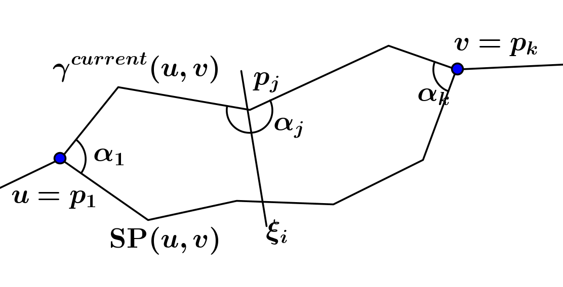
(i)

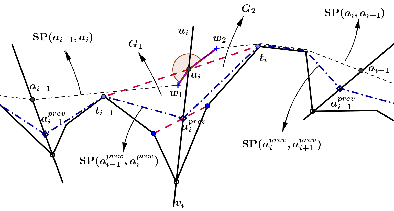
(ii)

Figure 9: (i): Illustration of the proof of Proposition 1 and (ii): illustration of the proof of Proposition 4 in the case $a_{i}^{prev}\neq a_{i}$

Lemma 2.

Recall that the upper angle created by ${\rm SP}(a_{i-1},a_{i})$ and ${\rm SP}(a_{i},a_{i+1})$ w.r.t. $[u_{i},v_{i}]$ is denoted by $\angle\left({\rm SP}(a_{i-1},a_{i}),{\rm SP}(a_{i},a_{i+1})\right)$. For $i=1,2,\ldots,N$, we suppose that $a_{i}\in]u_{i},v_{i}[$. Let $\hat{a_{i}}=\text{SP}(t_{i-1},t_{i})\cap[u_{i},v_{i}]$, where $t_{i-1}$ and $t_{i}$ are temporary points w.r.t. $a_{i-1}$ and $a_{i}$. Then we have

• $\angle\left({\rm SP}(a_{i-1},a_{i}),{\rm SP}(a_{i},a_{i+1})\right)=\pi\Leftrightarrow\hat{a_{i}}=a_{i}$;

• $\angle\left({\rm SP}(a_{i-1},a_{i}),{\rm SP}(a_{i},a_{i+1})\right)<\pi\Leftrightarrow\hat{a_{i}}\in]a_{i},u_{i}[$;

• $\angle\left({\rm SP}(a_{i-1},a_{i}),{\rm SP}(a_{i},a_{i+1})\right)>\pi\Leftrightarrow\hat{a_{i}}\in[v_{i},a_{i}[$.

Proof.

When Collinear Condition (B) does not hold, the role of $\hat{a_{i}}$ and $a_{i}^{next}$ are the same. By Proposition 2, Collinear Condition (B) in Sect. 3.3, and the fact that $a_{i}\neq v_{i}$, we get (a).

b) $(\Rightarrow)$ Suppose that $\angle\left(\text{SP}(a_{i-1},a_{i}),\text{SP}(a_{i},a_{i+1})\right)<\pi$ and $\hat{a_{i}}\notin]a_{i},u_{i}]$. Because $\text{SP}(t_{i-1},t_{i})$ never touches $B_{1}$ of $\mathcal{D}$, similarly to Remark 1, then $\hat{a_{i}}\neq u_{i}$. Therefore $\hat{a_{i}}\in[v_{i},a_{i}]$. Clearly, the collinear condition does not hold at $a_{i}$. Therefore $a_{i}\neq\hat{a_{i}}$, $\text{SP}(t_{i-1},t_{i})$ and $\text{SP}(t_{i-1},a_{i})\cup\text{SP}(a_{i},t_{i})$ are thus distinct. Then there are two distinct points $u,v$ which are common points to both $\text{SP}(t_{i-1},t_{i})$ and $\text{SP}(t_{i-1},a_{i})\cup\text{SP}(a_{i},t_{i})$ such that $\text{SP}(u,v)\cap\left(\text{SP}(u,a_{i})\cup\text{SP}(a_{i},v)\right)=\{u,v\}.$ Note that $\text{SP}(u,v)$ is also a sub-path of $\text{SP}(t_{i-1},t_{i})$. Then $\text{SP}(u,v)$ and $\text{SP}(u,a_{i})\cup\text{SP}(a_{i},v)$ form a simple polygon in $\mathcal{D}$ with $m$ vertices $p_{1}=u,p_{2},\ldots,p_{l}=a_{i},p_{l+1}\ldots,p_{k}=v,p_{k+1},\ldots,p_{m}$. Let $\alpha_{j}$ be the internal angle at $p_{j}$, with $j=1,2,\ldots,m$, see Fig 9(i). According to the property of shortest paths, $\alpha_{j}>\pi$ for $j\in\{1,2,\ldots,m\}\setminus\{1,k,l\}$. If $j=l$, due to $\alpha_{j}=2\pi-\angle\left(\text{SP}(a_{i-1},a_{i}),\text{SP}(a_{i},a_{i+1})\right)$, we have $\alpha_{j}>\pi$. Then $\alpha_{j}>\pi$ for $j\in\{1,2,\ldots,m\}\setminus\{1,k\}$. It is similar to the proof of Proposition 1, a contradiction is obtained. Thus $\hat{a_{i}}\in]a_{i},u_{i}[$.

c) $(\Rightarrow)$ Suppose that $\angle\left(\text{SP}(a_{i-1},a_{i}),\text{SP}(a_{i},a_{i+1})\right)>\pi$ and $\hat{a_{i}}\notin]v_{i},a_{i}[$. A contradiction can be deduced in much the same way as the above proof. Therefore $\hat{a_{i}}\in]v_{i},a_{i}[$.

b) c) $(\Leftarrow)$ For the sufficient condition of (b), ((c) can be considered similarly), assume that $\hat{a_{i}}\in]a_{i},u_{i}[$. Then $\angle\left(\text{SP}(a_{i-1},a_{i}),\text{SP}(a_{i},a_{i+1})\right)<\pi$, for if not, $\angle\left(\text{SP}(a_{i-1},a_{i}),\text{SP}(a_{i},a_{i+1})\right)\geq\pi$ deduces that $\hat{a_{i}}\in[v_{i},a_{i}]$ by the necessary conditions of (a) and (c) that are proved above, which is impossible. Hence the proof is complete. ∎

Proposition 4.

For all $j$, we have $\gamma^{j+1}$ is above $\gamma^{j}$ when we view from $B_{1}$, i.e., $a_{i}^{j+1}\in[a_{i}^{j},u_{i}[$, for $i=1,2,\ldots,N$, where $\gamma^{j}$ is the path obtained in $j^{th}$-iteration step of the algorithm.

Proof.

We give a proof by induction on $j$. The statement holds for $j=1$ due to taking initial shooting points $a_{i}^{0}=v_{i}$, for $i=1,2,\ldots,N$. Let $\{a_{i}^{prev}\}_{i=1}^{N},\{a_{i}\}_{i=1}^{N}$ and $\{a_{i}^{next}\}_{i=1}^{N}$ be the sets of shooting points corresponding to $k-1^{th}$, $k^{th}$ and $k+1^{th}$-iteration steps of the algorithm, respectively ($k\geq 1$). Assuming that, for $i=1,2,\ldots,N$, $a_{i}\in[a_{i}^{prev},u_{i}[$, we next prove that $a_{i}^{next}\in[a_{i},u_{i}[$.

If $\angle\left(\text{SP}(a_{i-1},a_{i}),\text{SP}(a_{i},a_{i+1})\right)\leq\pi$ due to Lemma 2(a) and (b), we obtain $a_{i}^{next}\in[a_{i},u_{i}[$. Thus we just need to prove that $a_{i}^{next}\in[a_{i},u_{i}[$ in the case $\angle\left(\text{SP}(a_{i-1},a_{i}),\text{SP}(a_{i},a_{i+1})\right)>\pi$. If $a_{i}=v_{i}$, then Collinear Condition (B) holds at $a_{i}$ then $a_{i}^{next}=a_{i}\in[a_{i},u_{i}[$. If $a_{i}\neq v_{i}$, suppose contrary to our claim, there is an index $i$ such that $\angle\left(\text{SP}(a_{i-1},a_{i}),\text{SP}(a_{i},a_{i+1})\right)>\pi$ and $a_{i}^{next}\notin[a_{i},u_{i}[$, i.e.,

$$a_{i}^{next}\in[v_{i},a_{i}[$$ (2)

Let $G_{1}$ be the closed region bounded by $[a_{i}^{prev},a_{i}]$, $\text{SP}(a_{i},t_{i-1})$ and $\text{SP}(t_{i-1},a_{i}^{prev})$. Let $G_{2}$ be the closed region bounded by $[a_{i}^{prev},a_{i}]$, $\text{SP}(a_{i},t_{i})$ and $\text{SP}(t_{i},a_{i}^{prev})$, where $t_{i-1}$ and $t_{i}$ are temporary points w.r.t. $a_{i-1}^{prev}$ and $a_{i}^{prev}$ (see Fig. 9(ii)). Since $a_{i}\in]u_{i},v_{i}[$, $\angle\left(\text{SP}(t_{i-1},a_{i}),\text{SP}(a_{i},t_{i})\right)=\pi$ by Lemma 1. Next, let $[a_{i},w_{1}]$ and $[a_{i},w_{2}]$ be segments having the common endpoint $a_{i}$ of $\text{SP}(a_{i-1},a_{i})$ and $\text{SP}(a_{i},a_{i+1})$, respectively. As $\angle\left(\text{SP}(t_{i-1},a_{i}),\text{SP}(a_{i},t_{i})\right)=\pi$ and $\angle\left(\text{SP}(a_{i-1},a_{i}),\text{SP}(a_{i},a_{i+1})\right)>\pi$, there are at least one of two following cases that will happen:

$$]a_{i},w_{1}]\text{ is below entirely }\text{SP}(t_{i-1},a_{i})$$ (3)

$$\text{ or }]a_{i},w_{2}]\text{ is below entirely }\text{SP}(a_{i},t_{i})\text{ when we view from }u_{i}.\hskip 113.81102pt$$

Then $\text{SP}(a_{i},t_{i})$, $\text{SP}(a_{i},a_{i+1})$ and $\text{SP}(a_{i}^{prev},t_{i})$ do not cross each other, due to the properties of shortest paths. According to Remark 3(a), for any temporary point $t_{i}\in\text{SP}(a_{i}^{prev},a_{i+1}^{prev})$, there is a polygon bounded by $[a_{i}^{prev},a_{i}]$, $[a_{i+1},a_{i+1}^{prev}]$, $\text{SP}(a_{i},a_{i+1})$, and $\text{SP}(a_{i}^{prev},a_{i+1}^{prev})$ which contains entirely $\text{SP}(a_{i},t_{i})$. Thus $\text{SP}(a_{i},a_{i+1})$ does not intersect with the interior of $G_{2}$. Similarly, $\text{SP}(a_{i-1},a_{i})$ does not also intersect with the interior of $G_{1}$. These things contradict (3), which completes the proof. ∎

Corollary 1.

Let $\gamma^{current}$ be the path obtained in some iteration step of the algorithm, where $\gamma^{current}=\cup_{i=0}^{N}{\rm SP}(a_{i},a_{i+1})$. If $a_{i}\in]v_{i},u_{i}[$, then we have $\angle\left({\rm SP}(a_{i-1},a_{i}),{\rm SP}(a_{i},a_{i+1})\right)\leq\pi$, for $i=1,2,\ldots,N$.

Lemma 3 (Proposition 5.1, [3]).

If $a,b,c,$ and $d$ are points in a simple polygon $\mathcal{P}$ such that $[a,d],[b,c]\subset\mathcal{P}$ , then $d_{\mathcal{H}}({\rm SP}(a,b),{\rm SP}(c,d))\leq\|a-d\|+\|b-c\|\leq 2\max\{\|a-d\|,\|b-c\|\}.$

Lemma 4 (Lemma 3.1, [9]).

If $\{a_{n}\}$ and $\{b_{n}\}$ are sequences of points in a simple polygon, $a_{n}\rightarrow a$ and $b_{n}\rightarrow b$, then $d_{\mathcal{H}}({\rm SP}(a_{n},b_{n}),{\rm SP}(a,b))\rightarrow 0$ as $n\rightarrow+\infty.$

The proof of Theorem 1:

Proof.

Let $\gamma^{j}=\cup_{i=0}^{N}\text{SP}(a_{i}^{j},a_{i+1}^{j})$, where $a_{i}^{j}\in[u_{i},v_{i}]$ for $i=1,2,\ldots,N$ and $a_{0}^{j}=\tilde{b},a_{N}^{j}=b$. If the algorithm stops after a finite number of iterations, the path obtained is the shortest. We thus just need to consider the case that $\{\gamma^{j}\}_{j\in\mathbb{N}}$ is infinite, according to Proposition 1.

For each $i=1,2,\ldots,N$, since $[u_{i},v_{i}]$ is compact and $\{a_{i}^{j}\}_{j\in\mathbb{N}}\subset[u_{i},v_{i}]$ there exists a sub sequence $\{a_{i}^{j_{k}}\}_{k\in\mathbb{N}}\subset\{a_{i}^{j}\}_{j\in\mathbb{N}}$ such that $\{a_{i}^{j_{k}}\}_{k\in\mathbb{N}}$ converges to a point, say $a_{i}^{*}$, in $\mathbb{R}^{2}$ with $\|.\|$ as $k\rightarrow\infty$. As $[u_{i},v_{i}]$ is closed, $\{a_{i}^{j_{k}}\}_{k\in\mathbb{N}}\subset[u_{i},v_{i}]$, and $\{a_{i}^{j_{k}}\}_{k\in\mathbb{N}}\rightarrow a_{i}^{*}$, we get $a_{i}^{*}\in[u_{i},v_{i}]$. Write $a_{0}^{*}=\tilde{b}$ and $a_{N+1}^{*}=b$. Set $\hat{\gamma}=\cup_{i=0}^{N}\text{SP}(a_{i}^{*},a_{i+1}^{*})$.

i.  We begin by proving the convergence of whole sequences,i.e., $\{a_{i}^{j}\}_{j\in\mathbb{N}}\rightarrow a_{i}^{*}$ as $j\rightarrow\infty$, for $i=1,2,\ldots,N$, based on the order of elements of $\{a_{i}^{j}\}_{j\in\mathbb{N}}$ shown in Proposition 4 and the convergence of their subsequence. By the order of elements of $\{a_{i}^{j}\}_{j\in\mathbb{N}}$ as shown in Proposition 4, for all natural numbers large enough $j$, there exits $k\in\mathbb{N}$ such that $a_{i}^{j}\in[a_{i}^{j_{k}},a_{i}^{j_{k+1}}]$. Furthermore, we also obtain $\{a_{i}^{j_{k}}\}_{k\in\mathbb{N}}$ converges on one side to $a_{i}^{*}$. For all $\delta>0$, there exists $k_{0}\in\mathbb{N}$ such that $\|a_{i}^{j_{k}}-a_{i}^{*}\|<\delta$, for $k\geq k_{0}$. As $a_{i}^{j}\in[a_{i}^{j_{k_{0}}},a_{i}^{*}]$, for $j\geq j_{k_{0}}$, we get $\|a_{i}^{j}-a_{i}^{*}\|<\delta$, for $j\geq j_{k_{0}}$. This clearly forces $\{a_{i}^{j}\}_{j\in\mathbb{N}}\rightarrow a_{i}^{*}$ as $j\rightarrow\infty$. This is the one-sided convergence, $\gamma^{j}$ is thus below $\hat{\gamma}$ when we view from the boundary $B_{1}$.

ii.  We next indicate that $d_{\mathcal{H}}(\gamma^{j},\hat{\gamma})\rightarrow 0$ as $j\rightarrow\infty$. According to item i, $a^{j}_{i}\rightarrow a_{i}^{*}$ as $j\rightarrow\infty$, for $i=1,2,\ldots,N$. By Lemma 4, we get $d_{\mathcal{H}}\left({\rm SP}(a^{j}_{i},a^{j}_{i+1}),{\rm SP}(a_{i}^{*},a_{i+1}^{*})\right)\rightarrow 0$ as $j\rightarrow\infty$. Note that $d_{\mathcal{H}}(A\cup B,C\cup D)\leq\max\{d_{\mathcal{H}}(A,C),d_{\mathcal{H}}(B,D)\}$, for all closed sets $A,B,C$ and $D$ in $\mathbb{R}^{2}$, we have $d_{\mathcal{H}}(\gamma^{j},\hat{\gamma})\leq\max_{0\leq i\leq N}\{d_{\mathcal{H}}\left({\rm SP}(a^{j}_{i},a^{j}_{i+1}),{\rm SP}(a_{i}^{*},a_{i+1}^{*})\right)\}.$ Therefore $d_{\mathcal{H}}(\gamma^{j},\hat{\gamma})\rightarrow 0$ as $j\rightarrow\infty$.

iii.  Our next claim is that $\hat{\gamma}$ is the shortest path joining $\tilde{b}$ and $b$. According to Proposition 1, we need to prove that Collinear Condition (B) holds at all $a_{i}^{*}$, for $i\in\{1,2,\ldots,N\}$. Conversely, suppose that there exists an index $i\in\{1,2,\ldots,N\}$ such that Collinear Condition (B) does not hold at $a_{i}^{*}$. If $a_{i}^{*}=v_{i}$ then $a_{i}^{j}=v_{i}$ for all $j\geq 0$. Then Collinear Condition (B) holds at $a_{i}^{j}$ for all $j\geq 0$, i.e., $\angle\left(\text{SP}(a_{i-1}^{j},a_{i}^{j}),\text{SP}(a_{i}^{j},a_{i+1}^{j})\right)\geq\pi$, for all $j\geq 0$. Since $\gamma^{j}$ is below $\hat{\gamma}$ when we view from the boundary $B_{1}$ and $\{a_{i-1}^{j}\}_{j\in\mathbb{N}}\rightarrow a_{i-1}^{*}$, $\{a_{i+1}^{j}\}_{j\in\mathbb{N}}\rightarrow a_{i+1}^{*}$ as $j\rightarrow\infty$, we get the upper angle of $\hat{\gamma}$ at $a_{i}^{*}$ is not less than $\pi$, which contradicts to Collinear Condition (B) not holding at $a_{i}^{*}$. Thus $a_{i}^{*}\neq v_{i}$. As Collinear Condition (B) does not hold at $a_{i}^{*}$, we conclude $\angle\left(\text{SP}(a_{i-1}^{*},a_{i}^{*}),\text{SP}(a_{i}^{*},a_{i+1}^{*})\right)<\pi$ or $\angle\left(\text{SP}(a_{i-1}^{*},a_{i}^{*}),\text{SP}(a_{i}^{*},a_{i+1}^{*})\right)>\pi.$

Case 1: $\angle\left(\text{SP}(a_{i-1}^{*},a_{i}^{*}),\text{SP}(a_{i}^{*},a_{i+1}^{*})\right)<\pi$. To obtain a contradiction, we will show that there exists a natural number $j_{0}$ such that the updating $a_{i}^{j_{0}}$ to $a_{i}^{j_{0}+1}$ gives $a_{i}^{j_{0}+1}\in(a_{i}^{*},u_{i}]$. Let $V$ be the set of all vertices of $\mathcal{D}$ which do not belong to $\hat{\gamma}$. Set

$$\mu=\min\left\{d(v,\hat{\gamma}):v\in V\right\}.$$ (4)

Because $V$ is finite, $d(v,\hat{\gamma})>0$, for $v\in V$, we get $\mu>0$. Let $\epsilon_{0}=\mu/4$. Since $a_{i}^{*}\neq v_{i}$, there is a point in $[v_{i},a_{i}^{*}]$, say $c_{i}$, such that $\|c_{i}-a_{i}^{*}\|=\epsilon_{0}$ (see Fig. 10(i)). Through $c_{i}$, we draw a polyline $\mathcal{L}$ whose line segments are parallel to line segments of $\text{SP}(a_{i-1}^{*},a_{i}^{*})\cup\text{SP}(a_{i}^{*},a_{i+1}^{*})$, respectively (see Fig. 10(ii)). Let us denote by $c_{i-1}$ ($c_{i+1}$, resp.) the point of intersection of $\mathcal{L}$ and the line going through $[u_{i-1},v_{i-1}]$ ($[u_{i+1},v_{i+1}]$, resp.). Since $a_{i}^{*}$ is very closed to $c_{i}$, w.l.o.g we can suppose that there is a line going through $a_{i}^{*}$ and creating with $\mathcal{L}$ an triangle, say $\triangle c_{i}dd^{\prime}$ (see Fig. 10(i)). If not, we can take

$$\epsilon_{0}=\dfrac{\mu}{2^{K_{0}}},\text{ where }K_{0}\text{ is a large enough natural number.}$$ (5)

For simplicity, assume that $\triangle c_{i}dd^{\prime}$ is an isosceles triangle, (see Fig. 10(i)).

Claim 1. Let $\alpha^{-}=\angle\left(\text{SP}(a_{i-1}^{*},a_{i}^{*}),[a_{i}^{*},u_{i}]\right)$ and $\alpha^{+}=\angle\left([a_{i}^{*},u_{i}],\text{SP}(a_{i}^{*},a_{i+1}^{*})\right)$. In $\triangle c_{i}dd^{\prime}$, we obtain

$$\|c_{i}-d\|=\epsilon_{0}.\dfrac{\sin\left(\frac{1}{2}(\pi-\alpha^{-}-\alpha^{+})\right)}{\sin\left(\frac{1}{2}(\pi-\alpha^{-}+\alpha^{+})\right)}.$$ (6)

The proof of Claim 1.

Using the Law of Sines in a triangle. ∎

Turning to the proof, for $i=1,2,\ldots,N$, since $\{a_{i}^{j}\}_{j\in\mathbb{N}}\rightarrow a_{i}^{*}$ as $j\rightarrow\infty$, there exists $\overline{j}\in\mathbb{N}$ such that

$$\|a_{i}^{j}-a_{i}^{*}\|<\dfrac{\epsilon_{0}}{M},\text{ for all }j\geq\overline{j},$$ (7)

where $M$ is a given real number which is chosen as in Claim 2 below and note that $M$ only depends on the segments $[u_{i-1},v_{i-1}],[u_{i},v_{i}]$, and $[u_{i+1},v_{i+1}]$.

Claim 2. If $[u_{i-1},v_{i-1}]$ is parallel to $[u_{i},v_{i}]$, then we set $m_{1}=1$. Otherwise let the point of intersection of two lines going through $[u_{i-1},v_{i-1}]$ and $[u_{i},v_{i}]$ be $s_{1}$ and we set $m_{1}=\dfrac{\|s_{1}-a_{i}^{*}\|}{\|s_{1}-a_{i-1}^{*}\|}$. Similarly, if $[u_{i+1},v_{i+1}]$ is parallel to $[u_{i},v_{i}]$, then we set $m_{2}=1$. Otherwise let the point of intersection of two lines going through $[u_{i+1},v_{i+1}]$ and $[u_{i},v_{i}]$ be $s_{2}$ and we set $m_{2}=\dfrac{\|s_{2}-a_{i}^{*}\|}{\|s_{2}-a_{i+1}^{*}\|}$. Take $M=\max\{1,m_{1},m_{2}\}$. Then ${\rm SP}(a_{i-1}^{j},a_{i}^{j})$ and ${\rm SP}(a_{i}^{j},a_{i+1}^{j})$ are contained in the region bounded by $\mathcal{L},[c_{i+1},a_{i+1}^{*}],{\rm SP}(a_{i-1}^{*},a_{i}^{*})\cup{\rm SP}(a_{i}^{*},a_{i+1}^{*})$, and $[a_{i-1}^{*},c_{i-1}]$, for all $j\geq\overline{j}$, where $\overline{j}$ is given by (7).

The proof of Claim 2.

For simplicity, we only prove the case that $[u_{i-1},v_{i-1}]$ is parallel to $[u_{i},v_{i}]$ and two lines going through $[u_{i+1},v_{i+1}]$ and $[u_{i},v_{i}]$ intersect at $s_{2}$ (see Fig. 10(ii)). One sees immediately that $m_{1}=1$ and $\|c_{i-1}-a_{i-1}^{*}\|=\|c_{i}-a_{i}^{*}\|=\epsilon_{0}$. By (7), we get $\|a_{i}^{j}-a_{i}^{*}\|<\epsilon_{0}$ and $\|a_{i-1}^{*}-a_{i-1}^{j}\|<\epsilon_{0}$. Therefore $\|a_{i}^{j}-a_{i}^{*}\|<\|c_{i}-a_{i}^{*}\|\text{ and }\|a_{i-1}^{*}-a_{i-1}^{j}\|<\|c_{i-1}-a_{i-1}^{*}\|.$ Besides, $\epsilon_{0}=\|c_{i}-a_{i}^{*}\|=\dfrac{\|s_{2}-a_{i}^{*}\|}{\|s_{2}-a_{i+1}^{*}\|}.\|c_{i+1}-a_{i+1}^{*}\|=m_{2}.\|c_{i+1}-a_{i+1}^{*}\|.$ Combining with (7) gives $\|a_{i+1}^{j}-a_{i+1}^{*}\|<\frac{\epsilon_{0}}{M}=\frac{m_{2}}{M}.\|c_{i+1}-a_{i+1}^{*}\|\leq\|c_{i+1}-a_{i+1}^{*}\|.$ These results yield the claim. ∎

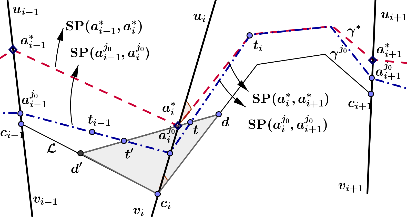
(i)

(ii)

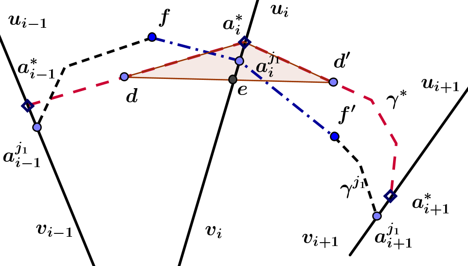
(iii)

Figure 10: Illustration of the proof of Theorem 1

We now turn to the proof of the theorem. We have $\angle\left(\text{SP}(a_{i-1}^{*},a_{i}^{*}),\text{SP}(a_{i}^{*},a_{i+1}^{*})\right)<\pi$ and the fact that $\{a_{i-1}^{j}\}$, $\{a_{i}^{j}\}$, and $\{a_{i+1}^{j}\}$ converge on one side to $a_{i-1}^{*}$, $a_{i}^{*}$ and $a_{i+1}^{*}$ as $j\rightarrow\infty$, respectively. There exists a natural number $j_{0}\geq\overline{j}$ such that $\angle\left(\text{SP}(a_{i-1}^{j_{0}},a_{i}^{j_{0}}),\text{SP}(a_{i}^{j_{0}},a_{i+1}^{j_{0}})\right)<\pi$. Then the algorithm updates $a_{i}^{j_{0}}$ to $a_{i}^{j_{0}+1}$. We are now in a position to show $a_{i}^{j_{0}+1}\in(a_{i}^{*},u_{i}]$.

Let two intersection points of $\gamma^{j_{0}}$ and $[d,d^{\prime}]$ be $t$ and $t^{\prime}$. By Lemma 3, $d_{\mathcal{H}}\left({\rm SP}(a^{j_{0}}_{i},a^{j_{0}}_{i+1}),{\rm SP}(a_{i}^{*},a_{i+1}^{*})\right)\leq 2\max\{\|a^{j_{0}}_{i}-a_{i}^{*}\|,\|a^{j_{0}}_{i+1}-a_{i+1}^{*}\|\}\leq\mu/2.$ Combining with (4), $\text{SP}(a_{i}^{j_{0}},a_{i+1}^{j_{0}})$ does not contain vertices of $V$ except the vertices belonging to $\hat{\gamma}$. Therefore, all endpoints of $\text{SP}(a_{i}^{j_{0}},a_{i+1}^{j_{0}})$ except for $a_{i}^{j_{0}}$ and $a_{i+1}^{j_{0}}$ belong to $\text{SP}(a_{i}^{*},a_{i+1}^{*})$. Note that the temporary point $t_{i}$ of $\gamma^{j_{0}}$ is taken as in step 4 of Procedure COLLINEAR_UPDATE($\gamma^{current},\gamma^{next},flag$). If $\text{SP}(a_{i}^{j_{0}},a_{i+1}^{j_{0}})$ is a line segment, we have $\|a_{i}^{j_{0}}-t_{i}\|\geq\frac{1}{2}d([u_{i},v_{i}],[u_{i+1},v_{i+1}]).$ Otherwise, $t_{i}$ is one of the endpoints of $\text{SP}(a_{i}^{j_{0}},a_{i+1}^{j_{0}})$ except for $a_{i}^{j_{0}}$ and $a_{i+1}^{j_{0}}$, and thus $t_{i}\in\hat{\gamma}$. Hence $\|a_{i}^{j_{0}}-t_{i}\|$ is greater than a given constant. As $\epsilon_{0}$ is given by (5), we have $t_{i}\notin[a_{i}^{j_{0}},t]$. Similarly, we also get $t_{i-1}\notin[a_{i}^{j_{0}},t^{\prime}]$. Because of the properties of shortest paths, $\text{SP}(t_{i-1},t_{i})$ do not intersect with $[t,t^{\prime}]$. In the sequence, $\text{SP}(t_{i-1},t_{i})$ intersects $[u_{i},v_{i}]$ in a point that is above $a_{i}^{*}$ when we see from $u_{i}$. This contradicts the result proved above in which $\gamma^{j_{0}+1}$ is below $\hat{\gamma}$ when we view from $B_{1}$.

Case 2: $\angle\left(\text{SP}(a_{i-1}^{*},a_{i}^{*}),\text{SP}(a_{i}^{*},a_{i+1}^{*})\right)>\pi$. Since $a_{i}^{*}\neq v_{i}$, there exist two points $d\in\text{SP}(a_{i-1}^{*},a_{i}^{*})$, and $d^{\prime}\in\text{SP}(a_{i}^{*},a_{i+1}^{*})$ such that three points $d,d^{\prime}$, and $a_{i}^{*}$ form a triangle that completely belongs to $\mathcal{D}$ but does not contain any vertex of $\mathcal{D}$, $[u_{i-1},v_{i-1}]\cap\triangle dd^{\prime}a_{i}^{*}=\emptyset$, and $[u_{i+1},v_{i+1}]\cap\triangle dd^{\prime}a_{i}^{*}=\emptyset$. Let $e=[d,d^{\prime}]\cap[u_{i},v_{i}]$.

We claim that there is no element of $\{a_{i}^{j}\}$ which is contained in $[e,a_{i}^{*}]$. Indeed, suppose that there exists $j_{1}\in\mathbb{N}$ such that $a_{i}^{j_{1}}\in[e,a_{i}^{*}]$. Let two segments having the common endpoint $a_{i}^{j_{1}}$ of $\gamma^{j_{1}}$ be $[f,a_{i}^{j_{1}}]$ and $[a_{i}^{j_{1}},f^{\prime}]$, where $f\in\text{SP}(a_{i-1}^{j_{1}},a_{i}^{j_{1}})$ and $f^{\prime}\in\text{SP}(a_{i}^{j_{1}},a_{i+1}^{j_{1}})$. Then either $f=a_{i-1}^{j_{1}}$ or $f$ is a vertex of $\mathcal{D}$, and hence $f\notin\triangle dd^{\prime}a_{i}^{*}$. Similarly, we get $f^{\prime}\notin\triangle dd^{\prime}a_{i}^{*}$. According to Corollary 1, it follows that $\angle{fa_{i}^{j_{1}}f^{\prime}}\leq\pi$. Because of $\angle ded^{\prime}=\pi$, we obtain either $[a_{i}^{j},f]$ crossing $[a_{i}^{*},d]$ or $[a_{i}^{j},f^{\prime}]$ crossing $[a_{i}^{*},d^{\prime}]$ (see Fig. 10(iii)). This contradicts the proved result that $\gamma^{j_{1}}$ is below $\hat{\gamma}$ when we view from the boundary $B_{1}$.

Summarizing, combining two cases gives that Collinear Condition (B) holds at $a_{i}^{*}$, for $i=1,2,\ldots,N$. Hence $\hat{\gamma}$ is the shortest path joining $\tilde{b}$ and $b$. The proof is complete. ∎

The proof of Theorem 2:

Proof.

(a) We have (see Figs. 4(iii) and (iv))

$$l(\gamma^{current})= \sum_{i=0}^{N}l(\text{SP}(a_{i},a_{i+1}))$$

$$= l(\text{SP}(a_{0},t_{0}))+\sum_{i=1}^{N}\left(l(\text{SP}(t_{i-1},a_{i}))+l(\text{SP}(a_{i},t_{i}))\right)+l(\text{SP}(t_{N},a_{N+1}))$$

$$\qquad\qquad\qquad\quad\geq \,l(\text{SP}(a_{0}^{next},t_{0}))+\sum_{i=1}^{N}l\left(\text{SP}(t_{i-1},t_{i})\right)+l(\text{SP}(t_{N},a_{N+1}^{next}))$$

$$= \,l(\text{SP}(a_{0}^{next},t_{0}))+\sum_{i=1}^{N}\left(l(\text{SP}(t_{i-1},a_{i}^{next}))+l(\text{SP}(a_{i}^{next},t_{i}))\right)+l(\text{SP}(t_{N},a_{N+1}^{next}))$$

$$= \sum_{i=0}^{N}\left(l(\text{SP}(a_{i}^{next},t_{i}))+l(\text{SP}(t_{i},a_{i+1}^{next}))\right)$$

$$\geq \sum_{i=0}^{N}\left(l(\text{SP}(a_{i}^{next},a_{i+1}^{next}))\right)=l\left(\cup_{i=0}^{N}\text{SP}(a_{i}^{next},a_{i+1}^{next})\right)=l(\gamma^{next}).$$

If Collinear Condition (B) does not hold at some shooting point $a_{i}$, then first inequality is strict. Thus $l(\gamma^{current})>l(\gamma^{next}).$

(b) Recall that $\gamma^{*}=\cup_{i=0}^{N}\text{SP}(a_{i}^{*},a_{i+1}^{*})$ is the shortest path joining $\tilde{b}$ and $b$ in $\mathcal{D}$ and $\gamma^{j}=\cup_{i=0}^{N}\text{SP}(a_{i}^{j},a_{i+1}^{j})$ is the sequence of paths obtained by the algorithm, where $a_{i}^{*}$ ($a_{i}^{j}$, resp.) is the intersection point between $\gamma^{*}$ ($\gamma^{j}$, resp.) and the corresponding cutting edge. If the algorithm stops after a finite number of iterations, the proof is trivial. Otherwise, repeat the proof of Theorem 1 (item i) we get $a^{j}_{i}\rightarrow a_{i}^{*}$ as $j\rightarrow\infty$, for $i=1,\ldots,N$, where $a^{j}_{0}=a_{0}^{*}$ and $a^{j}_{N+1}=a_{N+1}^{*}$. According to [[9], p. 542], the geodesic distance between two points $x$ and $y$ in a simple polygon, which is measured by the length of the shortest path joining two points $x$ and $y$ in the simple polygon, is a metric on the simple polygon and it is continuous as a function of both $x$ and $y$. That is, $l({\rm SP}(a_{i}^{j},a_{i+1}^{j}))\rightarrow l({\rm SP}(a_{i}^{*},a_{i+1}^{*}))$, for $i=0,1,\ldots,N$ as $j\rightarrow\infty$. It follows $l(\gamma^{j})\rightarrow l(\gamma^{*})$ as $j\rightarrow\infty$. ∎

The proof of Theorem 3:

Proof.

Steps 3 and 4 of the algorithm need $O(1)$ and $O(n)$ time, respectively. In step 5, there are at most two procedures of finding shortest paths in sub-polygons which call each vertex of $\mathcal{D}$. Since the problem of finding the shortest path joining two points in a simple polygon can be solved in linear time, computing the initial path $\gamma^{current}$ formed by the set of initial shooting points takes $O(n)$ time. Steps 8 and 9 need $O(1)$ time. We need to show that step 7 needs $O(n)$ time. For each iteration step, there are $N$ cutting segments, where $N$ is a given constant number, then the computing sequentially the angles at shooting points is done in constant time. In step 8 and 14 of for-loop in the procedure, since there are at most two procedures for finding the shortest path $\text{SP}(t_{i-1},t_{i})$ in sub-polygons $\mathcal{D}_{i-1}\cup\mathcal{D}_{i}$ which call each vertex of $\mathcal{D}$, time complexity of Procedure COLLINEAR_UPDATE($\gamma^{current},\gamma^{next},flag$) is linear. In summarizing, the algorithm runs in $O(kn)$ time, where $k$ is the number of iterations to get the required path. ∎

References

- [1] An, P. T. (2010). Reachable gasps on a polygon of a robot arm: finding the convex rope without triangulation, Journal of Robotics and Automation, 25(4), 304–310.
- [2] An, P. T. (2017). Optimization Approaches for Computational Geometry. Publishing House for Science and Technology, Vietnam Academy of Science and Technology, Hanoi, ISBN 978-604-913-573-6.
- [3] An, P. T., Hai, N. N., Hoai, T. V. (2013). Direct multiple shooting method for solving approximate shortest path problems. Journal of Computational and Applied Mathematics, 244, 67–76.
- [4] An, P. T., Hoai, T. V. (2012). Incremental convex hull as an orientation to solving the shortest path problem. International Journal of Information and Electronics Engineering, 2(5), 652–655.
- [5] An, P. T., Trang., L. H. (2018). Multiple shooting approach for computing shortest descending paths on convex terrains. Computational and Applied Mathematics, 37(4), 1–31.
- [6] An, P. T., Hai, N. N., Hoai, T. V., Trang., L. H. (2014). On the performance of triangulation-based multiple shooting method for 2D geometric shortest path problems. Transactions on Large-Scale Data- and Knowledge-Centered Systems XVI, 45–56.
- [7] Chazelle, B. (1982). A theorem on polygon cutting with applications, Proc. 23rd IEEE Symposium on Foundations of Computer Science, Chicago, 339–349.
- [8] Guibas, L., Hershberger, J., Leven, D., Sharir, M., Tarjan, R. E. (1987). Linear-time algorithms for visibility and shortest path problems inside triangulated simple polygons, Algorithmica, 2, 209–233.
- [9] Hai, N. N., An, P. T. (2011). Blaschke-type theorem and separation of disjoint closed geodesic convex sets. Journal of Optimization Theory and Applications, 151(3), 541-551.
- [10] Hai, N. N., An, P. T., & Huyen, P. T. T. (2019). Shortest paths along a sequence of line segments in euclidean spaces. Journal of Convex Analysis, 26(4), 1089-1112.
- [11] Heffernan, P. J., Mitchell, J. S. B. (1990). Structured visibility profiles with applications to problems in simple polygons, Proc. 6th Annual ACM Symp. Computational Geometry, 53–62.
- [12] Hoai, T. V. , An, P. T., Hai, N. N. (2017). Multiple shooting approach for computing approximately shortest paths on convex polytopes. Journal of Computational and Applied Mathematics, 317, 235–246.
- [13] Lee, D. T., Preparata, F. P. (1984). Euclidean shortest paths in the presence of rectilinear barriers, Networks, 14(3), 393–410.
- [14] Li. F, Klette. R. (2006). Finding the shortest path between two points in a simple polygon by applying a rubberband algorithm. In Pacific-Rim Symposium on Image and Video Technology. Springer, Heidelberg, 280–291.
- [15] Lozano-Perez, T. (1981). Automatic planning of manipulator transfer movements, IEEE Transactions on Systems, Man, and Cybernetics, SMC-11(10), 681-698.
- [16] Melkman, A. A. (1987). On-line construction of the convex hull of a simple polyline, Information Processing Letters, 25, 11–12.
- [17] Peshkin, M. A., Sanderson, A. C. (1986). Reachable grasps on a polygon: the convex rope algorithm, IEEE Journal on Robotics and Automation, 2(1), 5–58.
- [18] Song, P., Fu, Z., and Liu, L. (2018). Grasp planning via hand-object geometric fitting. The Visual Computer, 34(2), 257–270.
- [19] Toussaint, G. T. (1989). Computing geodesic properties inside a simple polygon, Revue d’Intelligence Artificielle, 3(2), 9–42.
- [20] Xue, Z., Zoellner, J. M., Dillmann, R. (2008). Automatic optimal grasp planning based on found contact points. International Conference on Advanced Intelligent Mechatronics, IEEE, 1053–1058.