GCS: Graph-Based Coordination Strategy for Multi-Agent Reinforcement Learning

Abstract.

Many real-world scenarios involve a team of agents that have to coordinate their policies to achieve a shared goal. Previous studies mainly focus on decentralized control to maximize a common reward and barely consider the coordination among control policies, which is critical in dynamic and complicated environments. In this work, we propose factorizing the joint team policy into a graph generator and graph-based coordinated policy to enable coordinated behaviours among agents. The graph generator adopts an encoder-decoder framework that outputs directed acyclic graphs (DAGs) to capture the underlying dynamic decision structure. We also apply the DAGness-constrained and DAG depth-constrained optimization in the graph generator to balance efficiency and performance. The graph-based coordinated policy exploits the generated decision structure. The graph generator and coordinated policy are trained simultaneously to maximize the discounted return. Empirical evaluations on Collaborative Gaussian Squeeze, Cooperative Navigation, and Google Research Football demonstrate the superiority of the proposed method. The code is available at https://github.com/Amanda-1997/GCS_aamas337.

1. Introduction

Multi-agent reinforcement learning (MARL) has shown exceptional results in many real-life applications, such as multiplayer games vinyals2017starcraft ; lowe2017maddpg , traffic control kuyer2008traffic , and social dilemmas leibo2017multi_social . A suitable control policy is extremely important in multi-agent systems (MASs). One choice is to treat the MAS as a single agent and adopt a centralized control policy han2019grid ; jiang2018atoc ; however, this approach is constrained by poor scalability for high-dimensional state and action spaces. On the contrary, decentralized control  sunehag2018vdn ; rashid2018qmix ; du2019liir ; lowe2017maddpg ; iqbal2019maac allows agents to make decisions independently, but struggles to enable coordinated behaviors on complex tasks. Taking traffic flow as an example, when multiple vehicles are trying to cross an intersection without traffic lights, most likely, the traffic will become congested if all vehicles take actions simultaneously without a rational sequence. This problem may be solved, however, if those vehicles move in an orderly way based on some coordination structure. This example shows that it is imperative to improve on a fully decentralized decision-making process, and a solution to alleviate the above issue is to develop a coordinated control policy to obtain cooperative behaviors.

Several approaches have been reported to address the problem of action coordination. BiAC zhang2020bilevel mainly focuses on coordination of the asynchronous decisions of two agents. The multi-agent rollout algorithm bertsekas2019multiagent_rollout provides a theoretical view of executing a local rollout with some coordinating information, but is limited to an agent-by-agent decision dependency structure. Although these works investigate the action execution order of two-agent and multi-agent systems, they are still insufficient to characterize the complicated and dynamic underlying decision dependency structure of a general multi-agent system. Moreover, we assert that representing the underlying decision dependency structure and using this to control the action execution is essential to improving coordination.

In this work, we propose a graph-based coordination strategy (GCS) that learns coordinated behaviors through factorizing the joint team policy into a graph generator and a graph-based coordinated policy. The former aims to learn an action coordination graph (ACG) that properly represents the decision dependency. The latter further coordinates the dependent behaviors among agents exploiting the underlying decision dependency. We train the graph generator and the graph-based coordinated policy simultaneously to maximize the discounted return. For the ACG we employ directed acyclic graphs (DAGs), whose nodes represent agents and whose directed edges denote action dependencies of the associated agents. Moreover, we propose using the DAGness-constrained and DAG depth-constrained optimization in the graph generator to balance efficiency and performance.

The contributions of this paper can be summarized as follows:

• As far as we know, we are the first to introduce directed acyclic graphs to action coordination, dynamically representing the underlying decision dependencies of MAS.

• We propose a DAGness-constrained and DAG depth-constrained optimization in the graph generator, achieving a trade-off between decision-making efficiency and performance.

• Empirical evaluations on several challenging MARL benchmarks (Collaborative Gaussian Squeeze, Cooperative Navigation, and Google Football) show that our method can achieve superior performance and obtain meaningful results consistent with intuitive expectations.

2. Related Work

Deep reinforcement learning has been successfully applied to addressing complex decision problems  (silver2017alphagozero, ; schrittwieser2020muzero, ; zhang2021population, ; wang2021ordering, ; meng2021offline, ). Due to the widespread existence of multi-agent tasks, MARL has attracted increasing attention, and learning appropriate control policies is important to obtain the maximum cumulative discounted return. Based on the structures of their execution schemes, we classify the existing approaches into three categories.

First, a fully independent execution scheme allows agents to determine actions according to their individual policies without any interaction. One line of research, such as IQL tan1993iql , VDN (sunehag2018vdn, ), QMIX (rashid2018qmix, ), and QTRAN (son2019qtran, ), focuses on value-based methods, which assign each agent an independent policy for execution. Another line of research, including MAAC (iqbal2019maac, ), COMA (foerster2018coma, ), and LIIR (du2019liir, ), extends the actor-critic algorithm degris2012actorcritic to the multi-agent case, where each actor represents an individual policy for an agent.

Second, the communication-based independent execution scheme is widely used, which allows the use of extensive information in its individual decision making (busoniu2008comprehensive_survey, ). In this scheme, agents learn how to transmit informative messages and to process the messages during training. Then agents exchange the messages to determine their actions individually during independent execution. Representative methods foerster2016RIALDIAL ; sukhbaatar2016CommNet ; zhang2013coordinating ; peng2017bicnet ; jiang2018atoc ; du2021flowcomm autonomously learn communication protocols that are required in generating informative messages: these determine whom to communicate with and what messages to transmit for assisted decision making.

Third, the coordinated execution scheme, where agents develop their policies conditioned on other agents’ actions and make decisions in a coordinated manner, is important in MAS. There are some methods that implicitly model the coordinated behaviours from the perspective of a coordination graph. DCG bohmer2020dcg uses pairwise graphs to propagate beliefs for joint decisions, while DICG li2021dicg focuses on generating a coordination graph with soft edge weights for message passing. DGN jiang2018dgn uses a graph attention network as an embedding extractor to assist in the decision making. Furthermore, some methods have been proposed to explicitly model the coordinated behaviours in order, such as Bi-AC (zhang2020bilevel, ) and multi-agent rollout (bertsekas2019multiagent_rollout, ), which propose utilizing two-agent and agent-by-agent dependency structures, respectively, to help agents make decisions in order and promote action coordination. Similar but essentially distinct, we introduce a mechanism to learn the underlying DAG structure that represents the decision dependency among agents.

Moreover, the generation of the DAGs is an essential part of our work. Recently, some continuous optimization approaches zheng2018dagsnotears ; yu2019daggnn ; yu2020dagsnocurl ; lachapelle2020gradientdag have been proposed to recover the DAGs through structure learning. The method zhu2019dagRL , closely related to our work, uses reinforcement learning as its search strategy to maximize a predefined score function. Borrowing from an idea of zhu2019dagRL , which obtains the DAG using reinforcement learning, we construct a graph generator module to generate the DAG structure as an action coordination graph and regard the extrinsic reward as the incentives to jointly train with MARL tasks.

3. Problem Setup

MMDPs

Cooperative multi-agent problems can be modeled as multiagent Markov decision processes (MMDPs) boutilier1996planning , which can be expressed as a tuple $<\{\mathcal{I}\},\mathcal{S},\{\mathcal{U}^{i}\}_{i=1}^{N},\mathbb{P},r,\gamma>$. $i\in\mathcal{I}$ is the $i^{th}$ player, $\mathcal{S}$ is the global state space, and $\mathcal{U}^{i}$ denotes the action space for the $i^{th}$ player. We label $\bm{u}:=(u^{1},...,u^{N})$ the joint actions for all players. Intuitively, the agent $i$ will select an individual action $u^{i}$ to perform and execute it. $\mathbb{P}$ is the transition dynamics, and $\mathbb{P}(\cdot|s,\bm{u})$ gives the distribution of the next state at state $s$ taking action $\bm{u}$. All agents share the same reward function $r(s,\bm{u}):s\times\bm{u}\to R$. $\gamma\in(0,1)$ denotes a discount factor, and $\tau=({s_{0}},{\bm{u}_{0}},{s_{1}},...)$ denotes the trajectory induced by the policy $\bm{\pi}=\{\pi^{i}\}_{i=1}^{N}$. All the agents coordinate together to maximize the cumulative discounted return ${\mathbb{E}_{\bm{\tau}\sim\pi}}\left[{\sum\nolimits_{t=0}^{\infty}{{\gamma^{t}}r({{s}_{t}},{\bm{u}_{t}})}}\right]$.

Factored MMDPs

We formalize our problem based on MMDPs as factored MMDPs. Different from MMDPs, where all actions are taken simultaneously and do not depend on each other, we endow the hierarchy order to the joint action based on the learned DAG structure $\mathcal{G}$, called an action coordination graph (ACG). The adjacency matrix $A$ representing the ACG denotes the decision dependency from the graph generator $\rho$. With $A$, we can define $\bm{\pi}=\prod\limits_{i=1}^{n}{\pi^{{i}}}({u^{i}}|{o^{i}},{u^{pa(i)}})$ as the graph-based coordinated policy for the $i^{th}$ player, where $o^{i}$ is the observation of the i-th player, $pa(i)$ are the parents of agent $i$, and ${u^{pa(i)}}$ are the actions taken by the parents, whose order is generated from $A$. Note that a fully decentralized policy is a special case of our graph-based coordinated policy where none of the agents have parents.

Figure 1 gives an example of the DAG and the relationships between nodes. The nodes in $\mathcal{G}$ correspond to the agents in the MAS, and the parent-child relationships represent the hierarchical decision dependencies among agents. For example, the case that the node $D$ in the graph has two parents $\{B,C\}$ illustrates that the action taken by the agent $D$ is constrained by $B$ and $C$.

Now, the graph-based coordination strategy is factorized as:

$$\pi(\bm{u},A|s)=\rho(A|s)\prod\limits_{i=1}^{n}{{\pi^{i}}({u^{i}}|{o^{i}},{u^{pa(i)\sim A}})},$$ (1)

where $\rho$ is the  graph generator, and $\pi^{i}$ is graph-based coordinated policy.

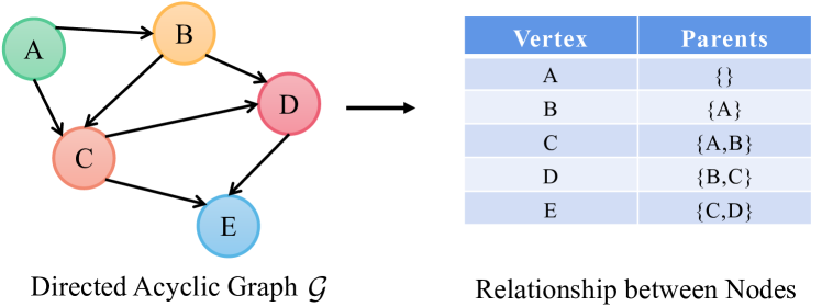
Figure 1. The left panel is a schematic diagram of a directed acyclic graph $\mathcal{G}$ with vertices $|\mathcal{V}|=5$ and edges $|\mathcal{E}|=7$. The right panel shows the parent–child relationships of $\mathcal{G}$.

4. Methodology

The overall goal is to maximize the cumulative return, denoted as:

$$\eta={\mathbb{E}_{A\sim\rho,\bm{u}\sim\pi(\cdot|s,A)}}\left[{\sum\limits_{k=0}^{\infty}{{\gamma^{k}}r({s_{t+k}},{\bm{u}_{t+k}})}}\right].$$ (2)

Now we further elaborate on the derivation of the graph-based coordinated policy ${\pi_{{\theta^{i}}}}({u^{i}}|{o^{i}},{u^{pa(i)}})$ and the graph generator  $\rho_{\varphi}(A|s)$, respectively.

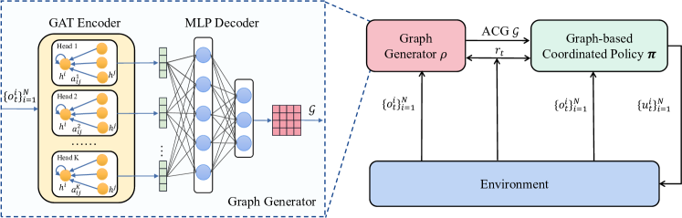
Figure 2. The proposed framework for the interaction process. The left is the graph generator including an encoder-decoder neural network model which is used to generate the DAG from the observed data.

4.1. Graph-based Coordinated Policy

Given a known graph generator $\rho$ (elaborated in Section 4.2), we have $A\sim\rho$ to represent the underlying decision dependency. Based on it, we can denote the decision policy as $\bm{\pi}=\prod\limits_{i=1}^{N}{{\pi^{i}}({u^{i}}|{o^{i}},{u^{pa(i)\sim A}})}$, called graph-based coordinated policy. We explore graph-based coordinated policy  $\bm{\pi}^{*}$ that obtains the final joint action $\{{u}^{i}\}_{i=1}^{N}$ as follows.

With Equations (1) and (2), we can write the expected return for agent $i$ as:

$$\begin{array}[]{l}\eta^{i}={\mathbb{E}_{s\sim{p^{\bm{\pi}}},(\bm{u},A)\sim\pi}}\left[{\pi(\bm{u},A|s)Q_{\bm{\pi}}^{i}(s,\bm{u})}\right]\\ ={\mathbb{E}_{s\sim{p^{\bm{\pi}}},{u^{i}}\sim{\pi^{i}},A\sim\rho}}\left[{\rho(A|s)\prod\limits_{i=1}^{N}{{\pi^{i}}({u^{i}}|{o^{i}},{u^{pa(i)\sim A}})}Q_{\bm{\pi}}^{i}(s,\bm{u})}\right].\end{array}$$ (3)

The graph-based coordinated policy $\bm{\pi}=\{\pi_{1},\pi_{2},...,\pi_{N}\}$ for $N$ agents can be parameterized by $\bm{\theta}=\{\theta_{1},\theta_{2},...,\theta_{N}\}$. Correspondingly, the gradient of the expected return for agent $i$ is expressed as:

$$\begin{array}[]{l}{\nabla_{{\theta^{i}}}}\eta({\theta^{i}})={\nabla_{{\theta^{i}}}}{\eta^{i}\vspace{2pt}}\\ ={\mathbb{E}_{s\sim{p^{\bm{\pi}}},u^{i}\sim\pi^{i}}}\left[{{\nabla_{{\theta^{i}}}}\log{\pi^{i}}({u^{i}}|{o^{i}},{u^{pa(i)}})\sum\nolimits_{A}{\rho(A|s)}Q_{\bm{\pi}}^{i}(s,\bm{u})}\right].\end{array}$$ (4)

By applying the mini-batch technique to the off-policy training, the gradient can be approximately estimated as:

$${\nabla_{{\theta^{i}}}}\eta({\theta^{i}})={\mathbb{E}_{(s,\bm{o},A,{\bm{u}})\sim\mathcal{D}}}\left[{{\nabla_{{\theta^{i}}}}\log{\pi^{i}}({u^{i}}|{o^{i}},{u^{pa(i)}})Q_{\bm{\pi}}^{i}(s,{\bm{u}})}\right],$$ (5)

where $\mathcal{D}$ is the experience replay buffer, recording experiences of all agents. Moreover, the centralized action-value function $Q_{\pi}^{i}$ can be updated as:

$${\mathcal{L}}(\phi)={E_{(s,\bm{o},A,{\bm{u}})\sim\mathcal{D}}}\left[{{{\left({Q_{\bm{\pi}}^{i}(s,\bm{u})-{y^{i}}}\right)}^{2}}}\right]$$ (6)

where ${y^{i}}=r+\gamma{\max_{\bm{u}^{\prime}}}Q_{{{\bm{\pi}}^{-}}}^{i}\left({s^{\prime},\bm{u}^{\prime}}\right)$ is the learning target and $Q_{{{\bm{\pi}}^{-}}}^{i}$ is the target network parameterized by $\theta^{i-}$.

During the training process, the graph-based coordinated policy  $\bm{\pi}=\{\pi_{1},\pi_{2},...,\pi_{N}\}$ and the  graph generator $\rho$ are updated iteratively. We will describe how to find the graph generator $\rho(\cdot)$ under a given policy $\bm{\pi}$.

4.2. Graph Generator

The graph generator aims to generate the DAG $\mathcal{G}$ to define the decision dependency among agents. We will introduce it in detail from three aspects: (a) DAGness constraint, (b) DAG Depth constraint, and (c) optimization objective.

DAGness constraint

The acyclicity constraint is an important issue in our problem setting. In this work, we also use the penalty terms like zheng2018dagsnotears ; lachapelle2020gradientdag ; zhu2019dagRL to ensure acyclicity. The result in zheng2018dagsnotears shows that the directed graph $\mathcal{G}$ with binary adjacency matrix $A$ is acyclic if and only if:

$$g(A):=\operatorname{trace}(e^{A\circ A})-d=0,$$ (7)

where $e^{A\circ A}$ is the matrix exponential, $A\circ A$ guarantees the non-negativity, and $d$ is the number of nodes in the DAGs. The ‘$\operatorname{trace}$’ of a matrix is defined as the sum of the diagonal elements zheng2018dagsnotears . The constraint function $g$ should satisfy that: (a) its derivatives are computable, and (b) $g$ can be the measurement of DAGs.

DAG Depth constraint

Moreover, taking the trade-off between efficiency and performance into account, we claim that the maximum depth of graph structure should be adjustable over different tasks. Therefore, we propose an alternative constraint to control the hierarchy of the generated DAGs as follows.

Definition 0.

A square matrix $A$ is a Nilpotent Matrix Algebra75 , if

$${A^{k}}=O\ and\ {A^{k-1}}\neq O,\ \exists k\in{\mathop{\rm\mathbb{Z^{+}}}},$$

where $O$ is the zero matrix and $A$ is called the Nilpotent of index $k$.

Proposition 0.

Let $A$ be an adjacency matrix for a directed acyclic graph, then the maximal length between any two nodes $i$ and $j$ is $k$ if $A$ is Nilpotent of index $k$.

We provide a detailed proof of proposition 2 in Appendix A.1. Here, we define ${c}(A^{k}):=sum({A^{k}})=\sum\nolimits_{i}{\sum\nolimits_{j}{A_{ij}^{k}=0}}$, which is equivalent to $A^{k}=O$. We remark that as long as constraint ${A^{k}}=O$ holds, it can be guaranteed that the maximal length between any two nodes $i$ and $j$ of the DAG does not exceed $k$.

Optimization objective.

Based on the foregoing, we can optimize $\rho$ parameterized by $\varphi$ with the maximal length $k$ by:

$$\begin{array}[]{l}\max\ \eta({\varphi})={\mathbb{E}}\left[{\sum\limits_{k=0}^{\infty}{{\gamma^{k}}r^{\rho}({s_{t+k}},{\bm{u}_{t+k}})}}\right]\vspace{2pt}\\ s.t.\ g(W)=0,{c}(W^{k})=0\end{array},$$ (8)

where $W=\rho_{\varphi}(\cdot)$ denotes the weight matrix generated from the graph generator $\rho$. Then the weight matrix is modeled as a Bernoulli distribution, from which the binary adjacency matrix $A$ is sampled. Here, we use the constraints of the weight matrix $g(W)$ and $c(W^{k})$ to approximate those of the adjacency matrix $g(A)$ and $c(A^{k})$ due to the consistency of representing the graph structure. With this approximation, we restate $\eta^{i}$ as:

$${\eta^{i}}=\mathbb{E}\left[{\rho\left({W|s}\right)\prod\limits_{i=1}^{N}{{\pi^{i}}\left({{u^{i}}|{o^{i}},{u^{pa(i)}}}\right)Q_{\bm{\pi}}^{i}(s,\bm{u})}}\right].$$ (9)

Fixing graph-based coordinated policy $\bm{\pi}$, we approximate the graph generator $\rho$ as follows. We augment the original problem shown in Equation (8) with a quadratic penalty using the augmented Lagrangian technique bertsekas1997nonlinear :

$$\begin{array}[]{l}\mathop{\min}\limits_{\varphi}\quad-\eta(\varphi)+\frac{\xi}{2}\left[{||g(W)||^{2}+||c({{W^{k}}})||^{2}}\right]\\ s.t.\quad g(W)=0,c({{W^{k}}})=0\end{array},$$ (10)

with the penalty $\xi>0$.

Next, we convert the Equation (10) to an unconstrained Lagrangian function:

$$\begin{array}[]{l}L(\varphi,{\lambda}_{1},{\lambda}_{2})=-\eta({\varphi})+\frac{\xi}{2}\left[{||g({W})||^{2}+||c\left({{{{W}}^{k}}}\right)||^{2}}\right]\\ \qquad\qquad\qquad+{\lambda}_{1}g({W})+{\lambda}_{2}c\left({{{{W}}^{k}}}\right)\\ \end{array}.$$ (11)

Proposition 0.

The gradient for Equation (11) to optimize the coordination graph generation policy can be derived as follows:

$$\begin{array}[]{l}\begin{array}[]{*{20}{l}}{{\nabla_{\varphi}}L({\varphi},{\lambda}_{1},{\lambda}_{2})={E_{s\sim p,W\sim\rho_{\varphi}(\cdot|s)}}\left[{{\nabla_{\varphi}}\log\rho_{\varphi}(W|s)\sum\limits_{{u^{i}}}{{{\pi}^{i}}({u^{i}}|{o^{i}},}}\right.\vspace{2px}}\\ {\qquad\qquad{u^{pa(i)}})\cdot{Q{{{}^{i}}}}({o^{i}},{u^{i}})-{{\lambda}_{1}}{{({e^{W^{\circ}W}})}^{T}}\cdot 2W-}\end{array}\vspace{2px}\\ \qquad\qquad\left.{{{\lambda}_{2}}{{\sum\nolimits_{i,j}{\left[{k{W^{k}}{W^{-1}}}\right]}}_{ij}}}\right],\end{array}$$

We provide a detailed proof of proposition 3 in Appendix A.2.

In proposition 3, we remark that after considering the influence of various decision dependencies on the reinforcement learning tasks, we can obtain the underlying graph structure that makes the best response to MARL tasks.

4.3. Implementation Details

As shown in Figure 2, the proposed framework include the graph-based coordinated policy and the graph generator, which will be elaborated below.

Graph-based Coordinated Policy

The graph-based coordinated policy can be obtained from the standard multi-agent actor-critic framework. As for the policy $\pi^{i}$ of the actor, we use the RNN network with the stochastic policy gradient to model the action distributions. The critic used to criticize the joint actions made by the actors is a three-layer feed-forward neural network activated by the ReLU units, denoted as $f_{critic}(o_{t},u_{t})=ReLU(\textit{MLP}\langle o_{t},u_{t}\rangle)$.

Graph Generator

As shown in Figure 2, the graph generator $\rho_{\varphi}(\bm{o})$ adopt an encoder-decoder module used to find the ACG. The GAT-based encoder can model the interplay of agents and extract the further latent representations. The MLP-based decoder is used to recover the pairwise relationship between agents to generate an ACG. The graph generator takes the local observations of the agents as input and outputs the ACG $\mathcal{G}$ to obtain the decision dependency for the decision-making process of the graph-based coordinated policy, elaborated as follows.

The graph generator contains two sub-modules. Firstly, we use the graph attention network (GAT) velivckovic2018gat as the attention-based encoder to extract the latent information for the graph structure generation. First, the simple feature is extracted by a multi-layer perceptron (MLP) as an initial step:

$${\{h_{t}^{i}\}}_{i=1}^{N}=f_{MLP}({\{o_{t}^{i}\}}_{i=1}^{N},{\{u_{t-1}^{i}\}}_{i=1}^{N}).$$ (12)

Due to the sufficiently expressive power of GAT, we use it to extract the further latent information of the simple feature. We compute the importance coefficients through the attention mechanism:

$$a_{t}^{ij}=\frac{{\exp(h_{t}^{i}\bm{W}{{(h_{t}^{j}\bm{W})}^{T}}/\sqrt{{d}}))}}{{\sum\nolimits_{k\in{{\{I\}}^{-i}}}{\exp(h_{t}^{i}\bm{W}{{(h_{t}^{k}\bm{W})}^{T}}/\sqrt{{d}})}}},\sum\nolimits_{j\in{{\{I\}}^{-i}}}{a_{t}^{ij}}=1,$$ (13)

where $\bm{W}\in R^{d{{}^{\prime}}\times d}$ is a learnable weight matrix, $d{{}^{\prime}}$ and $d$ denote the dimensions of the input vector and the latent vector, respectively, and $k\in{{\{I\}}^{-i}}$ indexes other agents except the agent $i$.

Then the multi-head attention is used to stabilize the learning process of self-attention, and the final latent feature is as follows:

$$h_{t}^{i^{\prime}}=\sigma\left({\frac{1}{M}\sum\limits_{m=1}^{M}{\sum\limits_{j\in{{\{I\}}^{-i}}}{a_{t,m}^{ij}{\bm{W}^{m}}h_{t}^{j}}}}\right).$$ (14)

where $M$ is the number of attention heads. $a_{t,m}^{ij}$ are importance coefficients computed by the k-th attention mechanism, and $W^{m}$ is the corresponding weight matrix.

Another sub-module in the graph generator is the decoder that generates a weight matrix used to sample the graph structure. Since the GAT-based encoder has already provided sufficiently expressive features among agents, a single-layer decoder is enough to easily construct the pairwise relationship between the encoder outputs to find a better structure of DAG for the decision policy.

$$f_{t}^{ij}(\bm{h}_{t}^{l},\bm{h}_{t}^{r},u)=\sigma(u^{T}tanh(\bm{W_{l}}\bm{h}_{t}^{l}+\bm{W_{r}}\bm{h}_{t}^{r})),$$ (15)

where $\bm{h}_{t}^{l}$ and $\bm{h}_{t}^{r}$ are agents’ higher-level representations from two encoder outputs, $\bm{W_{l}},\bm{W_{r}}\in\mathbb{R}^{d_{h}\times d_{e}},u\in\mathbb{R}^{d_{h}\times 1}$ are trainable parameters, and $d_{h},d_{e}$ are the hidden dimension and encoder output dimension, respectively.

Moreover, the logistic sigmoid function $\sigma(\cdot)$ generates the probability for constructing the Bernoulli distribution from which the binary adjacency matrix $A$ is sampled. The binary adjacency matrix forms a directed graph corresponding to the ACG $\mathcal{G}$. Here, we denote this graph generation process as $\mathcal{G}\sim\rho_{\varphi}(\bm{h})$.

Parameter Setting.

In the graph generator, the attention head in the GAT encoder is set to 8, the stacked attentional layers are set to 4, and the hidden units in the MLP is set to 64. In the graph-based coordinated policy, the actor critic architecture is adopted. The recurrent layer comprised of a GRU with a 64-dimensional hidden state, with a fully-connected layer before and after, is used as the actor. The critic is a two-layer MLP with the ReLu activation.

4.4. Algorithm Description

The main procedures are summarized in Algorithm 1, where ${\nabla_{\varphi}}L(\varphi)$, ${\eta_{{\theta^{i}}}}({\theta^{i}})$, and ${\nabla_{\phi}}\mathcal{L}(\phi)$ are optimized. Our ultimate goal is to obtain the graph-based coordinated policy  $\{\pi^{i}\}_{i=1}^{n}$. The graph generator $\rho$ is an intermediate used to access an excellent graph structure in guiding the decision-making sequence among agents to achieve a high degree of multi-agent coordination. The graph generator is a pluggable module that can be replaced by other algorithms for solving the DAGs. Note that DAGs are necessary because we need an execution structure that can determine a clear sequence of the actions, and therefore it should be directed and not circular. The policy solver is a universal module, which, in general, one can choose from a diverse set of cooperative MARL algorithms lowe2017maddpg ; yu2021mappo ; iqbal2019maac .

5. Experiments

We evaluate the effectiveness of our algorithm on three different environments: Collaborative Gaussian Squeeze son2019qtran , Cooperation Navigation lowe2017maddpg , and Google Research Football kurach2020google .

Ensure  graph-based coordinated policy $\pi^{i}$ and graph generator $\rho$;

Initialize $\epsilon,\gamma,M,C$, and the replay buffer $\mathcal{D}\leftarrow\emptyset$;

Initialize the parameters $\theta^{i},\phi^{i}$ for the graph-based coordinated policy networks, where $i=1,...,n$, and $\varphi$ for the graph generator network;

Initialize the target networks $\theta^{i^{-}}=\theta^{i}$ and $\phi^{i^{-}}=\phi^{i}$;

for each episode do

       Initial state $\leftarrow\{o_{0}^{i}\}_{i=1}^{n}$; // drop $i$ as $\bm{o_{0}}$ for clarity;

       Initialize $h_{0}^{(1)},...,h_{0}^{(n)}$ for RNN states;

       for each timestep $t$ do

             Get $\mathcal{G}_{t}\sim\rho(\cdot|\bm{o_{t}})$;

             Get the topological order $A_{t}=f(\mathcal{G}_{t})$;

             for $i$ in order $A_{t}$ do

                   augment the observations as $\hat{o}_{t}^{i}=(o_{t}^{i},u_{t-1}^{i},u_{t}^{pa(i)})$;

                   sample the action with $\epsilon$-greedy from $Q_{t}^{\pi^{i}}(\hat{o}_{t}^{i},u_{t}^{i};\theta^{i})$;

                   Update RNN state $h_{t}^{(1)},...,h_{t}^{(n)}$ $\leftarrow$ $h_{t-1}^{(1)},...,h_{t-1}^{(n)}$ ;

                   Receive reward ${\bm{r}_{t}}$ and observe next state ${\bf{o}}_{t+1}$;

                   Add transition $\{{\bm{o}}_{t},{\bm{u}}_{t},{\bm{r}}_{t},{\bm{o}}_{t+1}\}$ into $\mathcal{D}$;

             end for

            

       end for

      

      if  $episodes>M$ then

             Sample a minibatch $\mathcal{B}=\{{\bm{o}}_{j},{\bm{u}}_{j},{\bm{r}}_{j},{\bm{o}}_{j+1}\}^{M}_{j=0}\sim\mathcal{D}$ ;

             Update the policy $\pi^{i}$ using $\mathcal{B}$ and (4);

             Update the graph generator $\rho$ using $\mathcal{B}$ and ${\nabla_{\varphi}}L(\varphi)$;

             Update $\phi^{i}$ using (6);

             Every $C$ steps reset $\theta_{i}^{-}=\theta_{i}$ for $i=1,...,n$;

             Update the Lagrange penalty $\xi$ and the multipliers $\bm{\lambda}_{1},\bm{\lambda}_{2}$;

       end if

      

end for

Algorithm 1 The optimization of GCS.

5.1. Experimental Setting

Collaborative Gaussian Squeeze (CGS)

As an extension of Multi-domain Gaussian Squeeze (MGS) son2019qtran , Collaborative Gaussian Squeeze is a challenging environment for evaluating coordination. In MGS, there exist $K$ domains $[({\mu_{1}},{\sigma_{1}}),...,({\mu_{K}},{\sigma_{K}})]$ in the system. The system contains $N$ agents, and each agent $i$ can take actions $a_{i}$ within range of $\{-10,-9,..,0,1,..,8,9,10\}$. The prior $s_{i}\in[0,0.2]$ given by the environment represents the unit-level resource for each agent $i$. The total amount of resources mobilized by all agents is denoted as $f(\bm{u})=\sum\nolimits_{i}s_{i}\times a_{i}$. The goal is to maximize the joint reward $G(\bm{u})=\sum\nolimits_{k=1}^{K}{f(\bm{u}){e^{-{{(f(\bm{u})-{\mu_{k}})}^{2}}/{\sigma_{k}}^{2}}}}$. In our settings, we modify the original MGS to a collaborative task. We use two domains $[(\mu_{1}=5,\sigma_{1}=1.25),(\mu_{2}=-5,\sigma_{2}=1.25)]$. The computation of the joint reward is as follows:

$$G(\bm{u})=f(\bm{u}){e^{-{{(f(\bm{u})-{\mu_{1}})}^{2}}/{\sigma_{1}}^{2}}}-f(\bm{u}){e^{-{{(f(\bm{u})-{\mu_{2}})}^{2}}/{\sigma_{2}}^{2}}}.$$ (16)

Figure 3(a) shows the reward curves for this setting. According to the above definition, the reward is maximized when the resources of all the agents reach $\mu_{1}$ or $\mu_{2}$. In this environment, the social welfare depends on the intensity of collaboration.

Cooperative Navigation (CN)

Cooperative Navigation is a classic scenario implemented in the multi-agent particle world. This scenario has $n$ agents and $n$ landmarks, which are initialized with random locations at the beginning of each episode. The objective of the agents is to cooperate to cover all landmarks by controlling their velocities with directions. The action set $\mathcal{A}$ includes five actions: [up, down, left, right, stop]. Each agent can only observe its velocity, position, and displacement from other agents and the landmarks. The shared reward is the negative sum of displacements between each landmark and its nearest agent. Agents must also avoid collisions, since each agent is penalized with a ‘$-1$’ shared reward for every collision with other agents. We set the length of each episode as 25 time-steps. Therefore, the agents have to learn to navigate toward the landmarks cooperatively to cover all positions quickly and accurately. Figure 3(b) shows a classic scenario in Cooperative Navigation with $N=3$.

Google Research Football (GRF)

GRF is a realistically complicated and dynamic simulation environment without any clearly defined behavior abstraction, which is a suitable testbed for studying multi-agent decision making and coordination. In GRF, we use the Floats wrappers to represent the state. The Floats representation contains a 115-dimensional vector that summarizes the information, such as the ball position and possession, coordinates of all players, and the game state. Each player has 19 actions to control, including the standard move actions and different ball-kicking techniques. The rewards include the $SCORING$ reward $(-1,+1)$ and the $CHECKPOINT$ reward, which is the shaped reward that specifically addresses the sparsity of $SCORING$. Detailed descriptions are shown in Appendix B.

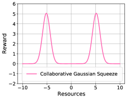
(a)

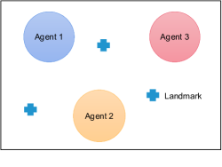
(b)

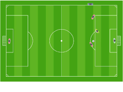
(c)

Figure 3. The schematics of our experimental environments.

Baselines

We compared our results with several baselines as follows. VDN and QMIX are state-of-the-art value factorization approaches that follow the regime of centralized training and decentralized execution, belonging to the class of fully decentralized control policies, with which it is difficult to obtain coordinated behaviours. DCG uses fully connected graphs for belief propagation, which only allows the message passing of paired agents. DGN aims at learning abstract representations to make simultaneous decisions.

• VDN sunehag2018vdn : Value Decomposition Network (VDN) imposes the structural constraint of additivity in the factorization, which represents $Q_{tot}$ as a sum of individual Q-values.

• QMIX rashid2018qmix : This was proposed to overcome the limitation that VDN uses the linear decomposition and ignores any extra state information available during training. QMIX enforces $Q_{tot}$ to be monotonic in the individual Q-values $Q^{i}$.

• DCG bohmer2020dcg : Deep Coordination Graph (DCG) factorizes the joint value function of all agents according to a coordination graph into payoffs between pairs of agents, which coordinates the actions between agents explicitly.

• DGN jiang2018dgn : DGN relies on a graph convolutional network to model the relation representations, implicitly modeling the action coordination.

5.2. Main Results

Here we report the experimental results from the setup described in Section 5.1. Performance validation indicates the superiority of introducing ACG to multi-agent systems.

Collaborative Gaussian Squeeze

In this game, there are 10 agents, and the maximum episode length is also set to 10. To emphasize the feasibility and effectiveness of our proposed framework, we first conduct the experiment on CGS. We report the average episode rewards over 10 random runs, shown in Figure 4. Our proposed algorithm GCS outperforms the baseline methods by a large margin. It can be seen that our algorithm handles the collaborative problem well; the action coordination graph facilitates behavior learning to promote cooperation. Next, we will verify the effectiveness of our algorithm on more complicated environments.

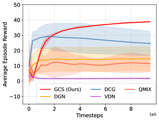
Figure 4. Average episode rewards compared with baselines on Collaborative Gaussian Squeeze.

Cooperative Navigation

As shown in Figure 3(b), Cooperative Navigation is a fully cooperative environment in which $N$ agents (circles) must cooperate to reach $N$ landmarks (crosses) with as few collisions as possible. We conduct experiments in Cooperative Navigation with $N=4$ and with $N=6$. Figures 5(a) and 5(b) show the learning curve comparisons for the two cases. We report the average episode reward at a training step, averaged over 10 independent running seeds.

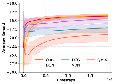
(a)

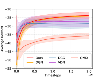
(b)

Figure 5. Average episode rewards for four agents and six agents in Cooperative Navigation.

First, our algorithm outperforms most baseline algorithms by giving higher converged rewards. We consider that our performance improvement results from the action coordination graph representing the action dependency for better coordination. Moreover, our algorithm converges fast during training, which is possibly because the hierarchical decision policies can efficiently induce coordination among agents in this cooperative setting. In addition, our algorithm can achieve a lower variance than those baselines, which indicates that the learned action coordination graph can reduce the uncertainty in decision making to facilitate cooperative behaviors among agents.

In contrast, VDN and QMIX take actions simultaneously without considering the action dependency among agents. They are faster during training, but that is of no benefit in inducing cooperation among agents. Additionally, DCG exhibits mediocre performance in this task. We believe that DCG considers only pairwise relationships between agents, which may disturb the overall balance in the system. In this case, DGN shows good performance consistent with ours, which shows that implicit action coordination modeling is also effective in pure cooperative settings.

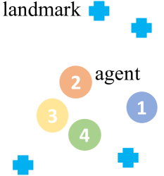
(a)

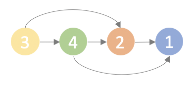
(b)

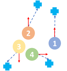
(c)

Figure 6. Illustration of the effects of the action coordination graph. (a) Current state. (b) Topological structure of the learned ACG. (c) The intention of agents according to the ACG. The dashed lines represent the targets, and the solid lines represent the actions.

In order to clearly show the meaningful effect of the action coordination graph in the decision-making process, we give a visualization at a time step in an episode of Cooperative Navigation, as shown in Figure 6. Figure 6(b) shows the topological structure of the learned ACG, and it suggests that the decision dependency of the agent is [3, 4, 2, 1]. The parent sets of the four agents are denoted as $pa(1)=\{4,2\}$, $pa(2)=\{3,4\}$, $pa(3)=\emptyset$, and $pa(4)=\{3\}$, respectively. First, agent 3 decides to move to the bottom-left landmark, then agent 4 takes the best response and decides to move to the bottom-right in order to avoid conflict with agent 3. After agent 2 knows the decisions of the previous two agents, it chooses the closer upper-left as its target instead of the bottom-right. Finally, agent 1 moves after observing the decisions of agents 2 and 4. This visualization shows how agents’ joint actions deriving from the ACG representing the underlying decision dependencies achieves efficiency.

Google Research Football (GRF)

To evaluate our method in complicated and dynamic environments, we conduct several experiments on GRF, as shown in Figure 7. In the 3-vs-2 scenario, three of our players try to score from the edge of the box, and the opponent team contains one defender and one keeper. In the 3-vs-6 scenario, there are six opponent players on the pitch to play against three of our players. In the 5-vs-5 scenario, each team has a keeper, an offensive player, and three defenders. Here, we report the average episode reward at a training step for each scenario, averaged over 10 independent running seeds.

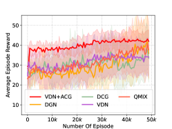
(a)

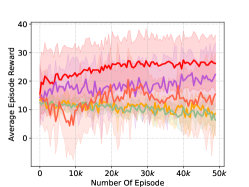
(b)

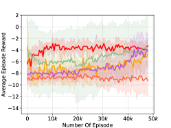
(c)

Figure 7. Average episode reward vs. training steps for comparisons with the baselines on Google Research Football.

As can be seen in Figure 7, our algorithm always obtains higher rewards than all the baselines in the different scenarios of GRF. This indicates that our method is quite general in complicated and dynamic environments. Moreover, this performance improvement in GRF demonstrates that our approach is good at effectively handling stochasticity and sparse rewards. This is because the learned ACG with the decision dependency is an efficient way to mitigate uncertainty and induce cooperation among agents. Taking the 3-vs-6 scenario for further demonstration, the training curve of QMIX fluctuates and is unstable, indicating this method’s inability to adapt to the dynamically complicated scenario with multiple opponent players. Here, DCG shows a trend of non-convergence, but our algorithm steadily rises to converge and obtains the highest reward, which exhibits the modeling supremacy of our approach for handling complicated tasks.

5.3. Results on DAG Depth

We observe that the inference efficiency and the performance gains are inversely affected by the ACG’s depth. Therefore, we aim to find the suitable depth $k$ that best balances the tradeoff. As shown in Figure 8, to validate the impact of the depth, we test our method on the Collaborative Gaussian Squeeze with different depth sizes of the learned ACG. In this figure, the horizontal axis is the depth, and the vertical axis is the testing episode reward averaged over five seeds. We test $1000$ episodes for each seed and obtain an average episode reward.

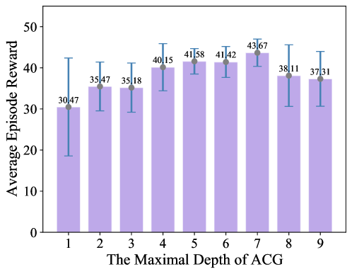
Figure 8. Effect of different DAG depth constraints on Collaborative Gaussian Squeeze.

As the depth of the ACG increases, the training time will increase correspondingly. However, the performance growth will gradually slow down, and performance degradation may even occur. In this case, $k=5$ is the optimal depth that balances the computational burden and the performance gains. As for the reason for the performance degradation with $k=8$ and $k=9$, we speculate that as the hierarchy of action dependency deepens, the complexity of the hypothesis space for the inference will increase, and it becomes harder to learn the optimal policy. In summary, a higher dependency level of the graph structure can provide more decision information to promote coordination and facilitate performance. However, this higher dependency level leads to a lower efficiency of inference, as the leaf node on the ACG needs to wait for all the parent nodes’ decisions before it makes its own decision.

5.4. Results on Dropping Edges

In this section, we verify the stability of the learned ACG in our proposed algorithm. Given a trained model with $depth=5$ on Collaborative Gaussian Squeeze, we evaluate 1000 episodes and count the average number of edges of ACG, denoted as $edges_{num}\approx 28$. A fair comparison requires the same depth and number of edges during training and evaluation. Therefore, we generate a fixed DAG structure $\mathcal{G}_{\{5,28\}}$, see Appendix C, whose depth is $5$ and whose number of edges is $28$, as the baseline to compare with our algorithm.

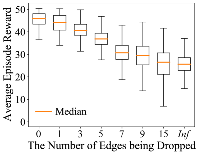
(a)

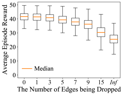
(b)

Figure 9. Box plots showing the distribution of the testing episode rewards in Collaborative Gaussian Squeeze.

In Figure 9, the horizontal axis represents the number of edges dropped from the generated or fixed graph structure, denoted as $\#drop$, and the vertical axis is the testing average episode reward over 1000 episodes. $Inf$ denotes dropping all the edges. The box plots visually show the distribution of the testing episode rewards and skewness by displaying the data quartiles. From the overall trend of Figure 9, we can observe that the data quartiles of the baseline reduce faster and change more drastically than our algorithm when the disturbance of edge dropping increases. This demonstrates that our algorithm has better stability. Moreover, in Table 1, our algorithm outperforms the baseline with higher mean rewards in most cases, which demonstrates the power of the ACG learned by our model to promote the coordination among agents reliably and stably even when confronted with disturbances of different intensities. It is worth noting that to guarantee stability, a slight performance loss may occur. It will be an interesting future research direction to study the stability–performance trade-off.

Table 1. Mean value of testing episode rewards when dropping corresponding numbers of edges.

	0	1	3	5	7	9	15	inf
The baseline	45.3	44.0	40.7	36.9	30.8	29.3	25.8	26.2
GCS (ours)	41.6	41.3	40.9	39.4	37.9	36.0	30.5	26.1

In summary, comparisons with VDN, QMIX, and DCG on three environments demonstrate that our algorithm achieves better performance, stronger stability, and more powerful modeling capability for handling dynamically complicated tasks than any of these methods. Moreover, the proposed DAG depth constraint provides an insightful view on balancing efficiency and performance.

6. Conclusions

In this paper, we introduce a novel graph generator  and graph-based coordinated policy in MARL to dynamically represent the underlying decision dependency structure and facilitate behavior learning, respectively. We propose the DAGness-constrained and DAG depth-constrained optimization to balance training efficiency and performance gains. Extensive empirical experiments on Collaborative Gaussian Squeeze, Cooperative Navigation, and Google Research Football, as well as comparisons to baseline algorithms, demonstrate the superiority of our method.

Future research may consider improving the limited performance by upgrading the graph generator model. We will also investigate an automatic mechanism for finding an appropriate depth for the action coordination graph.

Appendix A Detailed Proofs

We provide the detailed proofs of the propositions in the following.

A.1. Proof of Proposition 2

proof.

Firstly, we prove that the entry $A^{k}_{ij}$ in $k$-th power of the adjacency matrix $A$ indicates the number of walks of length $k$ from node $v_{i}$ to $v_{j}$. Let $\mathcal{L}^{l}(i,j)$ denote the number of walks of length $l$ from node $v_{i}$ to $v_{j}$. When $l=1$, $A^{1}=A,a_{ij}=\mathcal{L}^{1}(i,j)$. Let $b_{ij}=\mathcal{L}^{k}(i,j)$ denote the $ij^{th}$ entry of $A^{k}$. We have ${A_{ij}^{k+1}}=A_{ij}{A_{ij}^{k}}={a_{i1}}{b_{1j}}+{a_{i2}}{b_{2j}}+...+{a_{in}}{b_{nj}}=\sum\nolimits_{n}{{a_{in}}{b_{nj}}}$, where ${\forall_{m}}\in[1,n],{a_{im}}{b_{mj}}={\mathcal{L}^{1}}(i,m)\cdot{\mathcal{L}^{k}}(m,j)={\mathcal{L}^{k+1}}(i,j)$. So $A_{ij}^{k+1}$ denote the number of walks of length $k+1$ from $v_{i}$ to $v_{j}$. Then:

$$\begin{array}[]{l}{d}(A^{k}):=sum({A^{k}})=\sum\nolimits_{i}{\sum\nolimits_{j}{A_{ij}^{k}=0}}\\ {d}(A^{k-1}):=sum({A^{k-1}})=\sum\nolimits_{i}{\sum\nolimits_{j}{A_{ij}^{k-1}>0}}\end{array}.$$ (17)

The equations represent there is not a walk of length $k$ and there is at least one walk of length $k-1$ from $v_{i}$ to $v_{j}$ respectively, that is ${A^{k}}=O,{A^{k-1}}\neq O$. We define the hierarchy of the DAGs as the longest path length. Therefore, the hierarchy of the DAGs is $k$ if $A$ is the Nilpotent Matrix of index $k$. ∎

A.2. Proof of Proposition 3

Proof.

Let ${{{\pi}^{i}}}$ represent the fixed policy for agent $i$ trained by the graph-based coordinated policy. $\varphi$ is the parameter to be solved by the graph generator $\rho$. $g(\cdot)$ and $d(\cdot)$ are the constraint function as shown in Equation (7) and Equation (17). ${Q_{{{\pi}^{i}}}}(\cdot)$ denotes the state action function. The gradients is derived as follows.

$$\begin{array}[]{l}{\nabla_{\varphi}}L(\varphi,{\lambda_{1}},{\lambda_{2}})={\nabla_{\varphi}}\sum\limits_{s}{{p_{{{\pi}^{i}}}}(s)\sum\limits_{W}{\rho_{\varphi}(W|s)}\sum\limits_{{u^{i}}}{{{{\pi}^{i}}({u^{i}}|s,W)\cdot{{Q}_{{{\pi}^{i}}}}(s,{u^{i}})}}}\\ \left.{-{\lambda_{1}}g(W)-{\lambda_{2}}{d}(W^{k})}\right]\\ ={\nabla_{\varphi}}\sum\limits_{s}{{p_{{{\pi}^{i}}}}(s)\sum\limits_{W}{\rho_{\varphi}(W|s)}\sum\limits_{{u^{i}}}{\left[{{{\pi}^{i}}({u^{i}}|{o^{i}},{u^{pa(i)}})\cdot\left[{{Q_{{{\pi}^{i}}}}({o^{i}},{u^{i}})}\right.}\right.}}\\ \left.{-{\lambda_{1}}[tr({e^{W\circ W}})-d]-{\lambda_{2}}sum({W^{k}})}\right]\\ ={\mathbb{E}_{s\sim p,W\sim\rho_{\varphi}(\cdot|s)}}\left[{{\nabla_{\varphi}}\log\rho_{\varphi}(W|s)\sum\limits_{{u^{i}}}{{{\pi}^{i}}({u^{i}}|{o^{i}},{u^{pa(i)}})\cdot}{{Q_{{{\pi}^{i}}}}({o^{i}},{u^{i}})}}\right.\\ \left.{-{\lambda_{1}}{{({e^{W\circ W}})}^{T}}\cdot 2W-{\lambda_{2}}\sum\nolimits_{i,j}{{{\left[{k{W^{k}}{W^{-1}}}\right]}_{ij}}}}\right]\end{array}$$

∎

Appendix B Deatils of Google Research Football

Observations

The environment exposes the raw observations as Table 2. We use the Simple115StateWrapper as the simplified representation of a game state encoded with 115 floats.

Table 2. The main information and detailed descriptions about the observations in GRF.

Information	Descriptions
Ball information	position of ball
	direction of ball
	rotation angles of ball
	owned team of ball
	owned player of ball
Left team	position of players in left team
	direction of players in left team
	tiredness factor of players
	numbers of players with yellow card
	whether a player got a red card
	roles of players
Right team	position of players in right team
	direction of players in right team
	tiredness factor of players
	numbers of players with yellow card
	whether a player got a red card
	roles of players
Controlled player information	controlled player index
	designated player index
	active action
Match state	goals of left and right teams
	left steps
	current game mode
Screen	rendered screen

Actions

The number of actions available to an individual agent can be denoted as $|\mathcal{A}|=19$. The standard move actions (in $8$ directions) include $\mathcal{A}_{move}=\{Top,Bottom,Left,Right,Top-Left,Top-Right,Bottom-Left,Bottom-Right\}$. Moreover, the actions represent different ways to kick the ball is $\mathcal{A}_{kick}=\{ShortPass,HighPass,$
$LongPass,Shot,Do-Nothing,Sliding,Dribble,Stop-Dribble,Sprint,$
$Stop-Moving,Stop-Sprint\}$.

Rewards

The reward function mainly includes two parts. The first is $SCORING$, which corresponds to the natural reward where the team obtains $+1$ when scoring a goal and $-1$ when losing one to the opposing team. The second part is $CHECKPOINT$, which is proposed to address the issue of sparse rewards. It is encoded with domain knowledge by an additional auxiliary reward contribution. For example, we can increase the reward when the player owns the ball to boost passing the ball.

Appendix C The detailed structure of $\mathcal{G}_{\{5,28\}}$

The adjacency matrix of $\mathcal{G}_{\{5,28\}}$ is shown as follows.

$$\left[{\begin{array}[]{*{20}{c}}{0{\quad}1\quad 0\quad 1\quad 0\quad 1\quad 1\quad 0\quad 1\quad 0}\\ {0\quad 0\quad 0\quad 1\quad 0\quad 1\quad 1\quad 0\quad 1\quad 0}\\ {0\quad 1\quad 0\quad 1\quad 0\quad 1\quad 1\quad 0\quad 1\quad 0}\\ {0\quad 0\quad 0\quad 0\quad 0\quad 0\quad 0\quad 0\quad 0\quad 0}\\ {0\quad 1\quad 0\quad 1\quad 0\quad 0\quad 0\quad 0\quad 1\quad 0}\\ {0\quad 0\quad 0\quad 1\quad 0\quad 0\quad 0\quad 0\quad 1\quad 0}\\ {0\quad 0\quad 0\quad 0\quad 0\quad 0\quad 0\quad 0\quad 0\quad 0}\\ {0\quad 1\quad 0\quad 1\quad 0\quad 1\quad 1\quad 0\quad 1\quad 0}\\ {0\quad 0\quad 0\quad 0\quad 0\quad 0\quad 0\quad 0\quad 0\quad 0}\\ {0\quad 1\quad 0\quad 1\quad 0\quad 1\quad 0\quad 0\quad 1\quad 0}\end{array}}\right]$$

Appendix D Additional Experimental Details

We set discount factor $\gamma=0.99$. The optimization is conducted using RMSprop with a learning rate of $5\times 10^{-4}$ and $\alpha=0.99$ with no weight decay. Exploration for action selection is performed during training, and each agent executes $\epsilon-greedy$ policy over its actions. $\epsilon$ is annealed from $0.2$ to $0.05$ over the first $50k$ time steps and is kept constant afterwards.

In addition, the information regarding computational resources used is Enterprise Linux Server with 96 CPU cores and 6 Tesla K80 GPU cores(12G memory).

References

- [1] Oriol Vinyals, Timo Ewalds, Sergey Bartunov, Petko Georgiev, Alexander Sasha Vezhnevets, Michelle Yeo, Alireza Makhzani, Heinrich Küttler, John Agapiou, Julian Schrittwieser, et al. Starcraft ii: A new challenge for reinforcement learning. arXiv preprint arXiv:1708.04782, 2017.
- [2] Ryan Lowe, Yi Wu, Aviv Tamar, Jean Harb, Pieter Abbeel, and Igor Mordatch. Multi-agent actor-critic for mixed cooperative-competitive environments. pages 6382–6393, 2017.
- [3] Lior Kuyer, Shimon Whiteson, Bram Bakker, and Nikos Vlassis. Multiagent reinforcement learning for urban traffic control using coordination graphs. In Joint European Conference on Machine Learning and Knowledge Discovery in Databases, pages 656–671, 2008.
- [4] Joel Z Leibo, Vinicius Zambaldi, Marc Lanctot, Janusz Marecki, and Thore Graepel. Multi-agent reinforcement learning in sequential social dilemmas. In International Conference on Autonomous Agents and Multiagent Systems, pages 464–473, 2017.
- [5] Yali Du, Lei Han, Peng Sun, Jiechao Xiong, Qing Wang, Xinghai Sun, Han Liu, and Tong Zhang. Grid-wise control for multi-agent reinforcement learning in video game ai. In International Conference on Machine Learning (ICML), pages 1–9, 2019.
- [6] Jiechuan Jiang and Zongqing Lu. Learning attentional communication for multi-agent cooperation. Advances in Neural Information Processing Systems, 31:7254–7264, 2018.
- [7] Peter Sunehag, Guy Lever, Audrunas Gruslys, Wojciech Marian Czarnecki, Vinícius Flores Zambaldi, Max Jaderberg, Marc Lanctot, Nicolas Sonnerat, Joel Z Leibo, Karl Tuyls, et al. Value-decomposition networks for cooperative multi-agent learning based on team reward. In International Conference on Autonomous Agents and Multiagent Systems, pages 2085–2087, 2018.
- [8] Tabish Rashid, Mikayel Samvelyan, Christian Schroeder, Gregory Farquhar, Jakob Foerster, and Shimon Whiteson. Qmix: Monotonic value function factorisation for deep multi-agent reinforcement learning. In International Conference on Machine Learning, pages 4295–4304, 2018.
- [9] Yali Du, Lei Han, Meng Fang, Tianhong Dai, Ji Liu, and Dacheng Tao. Liir: learning individual intrinsic reward in multi-agent reinforcement learning. In Annual Conference on Neural Information Processing Systems, pages 4403–4414, 2019.
- [10] Shariq Iqbal and Fei Sha. Actor-attention-critic for multi-agent reinforcement learning. In International Conference on Machine Learning, pages 2961–2970, 2019.
- [11] Haifeng Zhang, Weizhe Chen, Zeren Huang, Minne Li, Yaodong Yang, Weinan Zhang, and Jun Wang. Bi-level actor-critic for multi-agent coordination. In AAAI Conference on Artificial Intelligence, pages 7325–7332, 2020.
- [12] Dimitri Bertsekas. Multiagent rollout algorithms and reinforcement learning. arXiv preprint arXiv:1910.00120, 2019.
- [13] David Silver, Julian Schrittwieser, Karen Simonyan, Ioannis Antonoglou, Aja Huang, Arthur Guez, Thomas Hubert, Lucas Baker, Matthew Lai, Adrian Bolton, et al. Mastering the game of go without human knowledge. Nature, 550:354–359, 2017.
- [14] Julian Schrittwieser, Ioannis Antonoglou, Thomas Hubert, Karen Simonyan, Laurent Sifre, Simon Schmitt, Arthur Guez, Edward Lockhart, Demis Hassabis, Thore Graepel, et al. Mastering atari, go, chess and shogi by planning with a learned model. Nature, 588:604–609, 2020.
- [15] Duzhen Zhang, Tielin Zhang, Shuncheng Jia, Xiang Cheng, and Bo Xu. Population-coding and dynamic-neurons improved spiking actor network for reinforcement learning. arXiv preprint arXiv:2106.07854, 2021.
- [16] Xiaoqiang Wang, Yali Du, Shengyu Zhu, Liangjun Ke, Zhitang Chen, Jianye Hao, and Jun Wang. Ordering-based causal discovery with reinforcement learning. In Zhi-Hua Zhou, editor, Proceedings of the Thirtieth International Joint Conference on Artificial Intelligence, IJCAI-21, pages 3566–3573. International Joint Conferences on Artificial Intelligence Organization, 8 2021.
- [17] Linghui Meng, Muning Wen, Yaodong Yang, Chenyang Le, Xiyun Li, Weinan Zhang, Ying Wen, Haifeng Zhang, Jun Wang, and Bo Xu. Offline pre-trained multi-agent decision transformer: One big sequence model conquers all starcraftii tasks. arXiv preprint arXiv:2112.02845, 2021.
- [18] Ming Tan. Multi-agent reinforcement learning: Independent vs. cooperative agents. In International Conference on Machine Learning, pages 330–337, 1993.
- [19] Kyunghwan Son, Daewoo Kim, Wan Ju Kang, David Hostallero, and Yung Yi. QTRAN: learning to factorize with transformation for cooperative multi-agent reinforcement learning. In International Conference on Machine Learning, pages 5887–5896, 2019.
- [20] Jakob N. Foerster, Gregory Farquhar, Triantafyllos Afouras, Nantas Nardelli, and Shimon Whiteson. Counterfactual multi-agent policy gradients. In AAAI Conference on Artificial Intelligence, pages 2974–2982, 2018.
- [21] Thomas Degris, Martha White, and Richard S Sutton. Off-policy actor-critic. arXiv preprint arXiv:1205.4839, 2012.
- [22] Lucian Busoniu, Robert Babuska, and Bart De Schutter. A comprehensive survey of multiagent reinforcement learning. IEEE Transactions on Systems, Man, and Cybernetics, Part C (Applications and Reviews), 38(2):156–172, 2008.
- [23] Jakob N Foerster, Yannis M Assael, Nando de Freitas, and Shimon Whiteson. Learning to communicate with deep multi-agent reinforcement learning. In Annual Conference on Neural Information Processing Systems, pages 2145–2153, 2016.
- [24] Sainbayar Sukhbaatar, Arthur Szlam, and Rob Fergus. Learning multiagent communication with backpropagation. In Annual Conference on Neural Information Processing Systems, pages 2252–2260, 2016.
- [25] Chongjie Zhang and Victor Lesser. Coordinating multi-agent reinforcement learning with limited communication. In International Conference on Autonomous Agents and Multi-Agent Systems, pages 1101–1108, 2013.
- [26] Peng Peng, Quan Yuan, Ying Wen, Yaodong Yang, Zhenkun Tang, Haitao Long, and Jun Wang. Multiagent bidirectionally-coordinated nets for learning to play starcraft combat games. CoRR, abs/1703.10069, 2017.
- [27] Yali Du, Bo Liu, Vincent Moens, Ziqi Liu, Zhicheng Ren, Jun Wang, Xu Chen, and Haifeng Zhang. Learning correlated communication topology in multi-agent reinforcement learning. In International Conference on Autonomous Agents and Multi-Agent Systems, pages 456–464, 2021.
- [28] Wendelin Böhmer, Vitaly Kurin, and Shimon Whiteson. Deep coordination graphs. In International Conference on Machine Learning, pages 980–991, 2020.
- [29] Sheng Li, Jayesh K Gupta, Peter Morales, Ross Allen, and Mykel J Kochenderfer. Deep implicit coordination graphs for multi-agent reinforcement learning. In International Conference on Autonomous Agents and MultiAgent Systems, pages 764–772, 2021.
- [30] Jiechuan Jiang, Chen Dun, Tiejun Huang, and Zongqing Lu. Graph convolutional reinforcement learning. arXiv preprint arXiv:1810.09202, 2018.
- [31] Xun Zheng, Bryon Aragam, Pradeep K Ravikumar, and Eric P Xing. Dags with no tears: Continuous optimization for structure learning. Annual Conference on Neural Information Processing Systems, pages 9472–9483, 2018.
- [32] Yue Yu, Jie Chen, Tian Gao, and Mo Yu. Dag-gnn: Dag structure learning with graph neural networks. In International Conference on Machine Learning, pages 7154–7163, 2019.
- [33] Yue Yu and Tian Gao. Dags with no curl: Efficient dag structure learning. In Annual Conference on Neural Information Processing Systems, 2020.
- [34] Sébastien Lachapelle, Philippe Brouillard, Tristan Deleu, and Simon Lacoste-Julien. Gradient-based neural dag learning. 2020.
- [35] Shengyu Zhu, Ignavier Ng, and Zhitang Chen. Causal discovery with reinforcement learning. In International Conference on Learning Representations, 2019.
- [36] Craig Boutilier. Planning, learning and coordination in multiagent decision processes. In Theoretical Aspects of Rationality and Knowledge, volume 96, pages 195–210, 1996.
- [37] I. N. Herstein. Topics In Algebra. John Wiley & Sons, 2nd edition, 1975.
- [38] Dimitri P Bertsekas. Nonlinear programming. Journal of the Operational Research Society, 48:334–334, 1997.
- [39] Petar Veličković, Guillem Cucurull, Arantxa Casanova, Adriana Romero, Pietro Liò, and Yoshua Bengio. Graph attention networks. In International Conference on Learning Representations, 2018.
- [40] Chao Yu, Akash Velu, Eugene Vinitsky, Yu Wang, Alexandre Bayen, and Yi Wu. The surprising effectiveness of mappo in cooperative, multi-agent games. arXiv preprint arXiv:2103.01955, 2021.
- [41] Karol Kurach, Anton Raichuk, Piotr Stańczyk, Michał Zaj\kac, Olivier Bachem, Lasse Espeholt, Carlos Riquelme, Damien Vincent, Marcin Michalski, Olivier Bousquet, et al. Google research football: A novel reinforcement learning environment. In AAAI Conference on Artificial Intelligence, pages 4501–4510, 2020.