Understanding the phase reversals of Galactic cosmic ray anisotropies

Abstract

The energy spectra and anisotropies are very important probes of the origin of cosmic rays. Recent measurements show that complicated but very interesting structures exist, at similar energies, in both the spectra and energy-dependent anisotropies, indicating a common origin of these structures. Particularly interesting phenomenon is that there is a reversal of the phase of the dipole anisotropies, which challenges a theoretical modeling. In this work, for the first time, we identify that there might be an additional phase reversal at $\sim 100$ GeV energies of the dipole anisotropies as indicated by a few underground muon detectors and the first direct measurement by the Fermi satellite, coincident with the hundreds of GV hardenings of the spectra. We propose that these two phase reversals, together with the energy-evolution of the amplitudes and spectra, can be naturally explained with a nearby source overlapping onto the diffuse background. As a consequence, the spectra and anisotropies can be understood as the scalar and vector components of this model, and the two reversals of the phases characterize just the competition of the cosmic ray streamings between the nearby source and the background. The alignment of the cosmic ray streamings along the local large-scale magnetic field may play an important but sub-dominant role in regulating the cosmic ray propagation. More precise measurements of the anisotropy evolution at both low energies by space detectors and high energies by air shower experiments for individual species will be essential to further test this scenario.

1 Introduction

The origin of Galactic cosmic rays (GCRs), after more than one century of their first discovery, remains one of the most interesting mysteries in astrophysics. Directly identifying the sources of GCRs is difficult, since those charged particles propagate diffusively in the turbulent magnetic field of the Milky Way, losing largely their original directions. The information of the sources and the propagation process can imprint in the energy spectra and the tiny anisotropies of GCRs (Blasi, 2013; Grenier et al., 2015; Ahlers & Mertsch, 2017). Precise measurements of the spectra and anisotropies of GCRs, particularly for various species, are thus very important in probing the origin of GCRs.

There have been quite a lot of efforts in measuring the anisotropies of arrival directions of GCRs, at large and small scales, by underground and ground-based experiments (Amenomori et al., 2005; Guillian et al., 2007; Abdo et al., 2009; Abbasi et al., 2010, 2012; Aartsen et al., 2013; Bartoli et al., 2015; Amenomori et al., 2017; Bartoli et al., 2018; Amenomori et al., 2006; Abdo et al., 2008; Amenomori et al., 2010; Abbasi et al., 2011; Bartoli et al., 2013; Abeysekara et al., 2014; Aartsen et al., 2016; Abeysekara et al., 2019). The dominant component of the anisotropies is approximately a dipole, with amplitudes being $10^{-4}\sim 10^{-3}$ for energies below PeV and experiencing a complicated rising-declining-rising energy-dependence. The phase of the dipole anisotropies shows a reversal at $\sim 100$ TeV when the amplitude reaches the minimum. For $E\lesssim 100$ TeV, the phase is aligned approximately with the local interstellar magnetic field as inferred by IBEX measurements of the neutral atoms (Schwadron et al., 2014), and at higher energies the phase turns to the Galactic center (GC) direction.

The explanation of the GCR anisotropies is a challenge for a long time. The conventional GCR production and propagation model with diffusion coefficients obtained from fitting the B/C ratio predicts in general a power-law rising of the dipole amplitude which is significantly higher than the measurements (Strong et al., 2007). The predicted dipole phase of the conventional model is from the GC to the anti-GC direction which also differs from the data (Strong et al., 2007). The observed energy-dependence of the amplitude and phase thus triggers a lot of discussion of possible effects from discrete sources and/or large scale magnetic fields (Erlykin & Wolfendale, 2006; Blasi & Amato, 2012; Pohl & Eichler, 2013; Sveshnikova et al., 2013; Kumar & Eichler, 2014; Mertsch & Funk, 2015; Savchenko et al., 2015; Ahlers, 2016). For example, Savchenko et al. (2015) illustrated that the dipole anisotropies of GCRs could be reproduced assuming a superposition of a local source with an age of 2 Myr and a distance of $\sim$200 pc, and the contribution from the background GCR sea.

Recently, new observations of the energy spectra of GCRs and $\gamma$ rays shed new light on the understanding of the anisotropies and further on the origin of GCRs. Precise measurements of the energy spectra of protons and helium nuclei show hardening features around several hundred GV rigidities and subsequent softening features around $\sim 10$ TV (Aguilar et al., 2015b, a; An et al., 2019; Alemanno et al., 2021). It is very interesting to note that the spectral structures of the fluxes may co-evolve with the anisotropies, indicating common origins of those structures (Liu et al., 2019; Qiao et al., 2019). In addition, the extended $\gamma$-ray morphologies around middle-aged pulsars, known as pulsar halos, suggest that the diffusion of high-energy particles in the surroundings of pulsars is much slower than the average diffusion velocity in the Milky Way (Abeysekara et al., 2017; Aharonian et al., 2021). The spatial variations of the GCR intensities and spectral indices inferred from the Fermi $\gamma$-ray observations also suggest the propagation of GCRs is inhomogeneous throughout the Milky Way (Yang et al., 2016; Acero et al., 2016). A spatially inhomogeneous propagation scenario plus a nearby source was proposed, which naturally explains the new phenomena of GCR spectra and $\gamma$ rays, as well as the anisotropies (Liu et al., 2019; Qiao et al., 2019).

The key point of the above scenario to account for the phase reversal of the dipole anisotropies at $\sim 100$ TeV is the competition of the GCR streamings between the background sources (from the GC to the anti-GC direction, dominating above 100 TeV) and the nearby source (from the source direction to the opposite direction, dominating below 100 TeV). The projection of the streamings along the local magnetic field may affect the exact values of the dipole phase (Ahlers, 2016), but the overall picture keeps applicable. A natural expectation of this scenario is that there should be an additional phase reversal at low energies when the background streaming dominates again since the background GCR spectrum is softer than the local source. It is very interesting to note that the first direct measurement of the all-sky anisotropies by space satellite Fermi seems to observe this predicted reversal of the dipole component at $\sim 100$ GeV energies, although the significance is not high enough to robustly claim a detection (Ajello et al., 2019). The Fermi data shows a dipole amplitude of $(3.9\pm 1.5)\times 10^{-4}$ and a phase of $-9.7\pm 1.5$ hr in the Right Ascension (R.A.) when projecting to one-dimension on R.A., for protons with $E>78$ GeV (Ajello et al., 2019). The phase of Fermi result differs by nearly 12 hr from those measured by underground muon detectors above 100 GeV, and just experiences a reversal.

2 Model Description

2.1 The propagation of GCRs

The propagation of GCRs in the Milky Way is naturally expected to be inhomogeneous due to the spatial variations of the physical parameters of the interstellar medium (ISM). The non-linear feedback of GCRs on the ISM turbulence may further enhance the spatial inhomogeneities of the GCR transportation (Blasi et al., 2012; Recchia et al., 2016). The observations of $\gamma$-rays by HAWC, and LHAASO offer direct evidence in support of such a scenario (Abeysekara et al., 2017; Aharonian et al., 2021). In this work we adopt a two-halo description of the spatially-dependent propagation (SDP) of GCRs (Tomassetti, 2012; Guo et al., 2016). Here, the two propagation halos are defined as the inner halo (disk) and outer halo. The diffusion in the inner halo is much slower than that in the outer one. The diffusion coefficient can be parameterized as

$$D_{xx}(r,z,{\cal R})=D_{0}F(r,z)\beta^{\eta}\left(\dfrac{\cal R}{{\cal R}_{0}}\right)^{\delta_{0}F(r,z)},$$ (1)

where ${\cal R}$ is the particle’s rigidity, ${\cal R}_{0}\equiv 4$ GV, $D_{0}$ and $\delta_{0}$ are constants representing the diffusion coefficient in the outer halo, $\eta$ is a phenomenological constant employed to fit the low-energy spectra. The spatial-dependent function $F(r,z)$ is defined as (Guo et al., 2016),

$$F(r,z)=\left\{\begin{array}[]{ll}{g(r,z)+[1-g(r,z)]}\left(\dfrac{{z}}{\xi{z_{h}}}\right)^{n},&{{|z|}\leq\xi{z_{h}}}\\ 1,&{{|z|}>\xi{z}_{\rm h}}\\ \end{array},\right.$$ (2)

where $g(r,z)$=$N_{m}$/[1+$f(r,z)$] with $f(r,z)$ being the GCR source distribution, $z_{h}$ is the half-thickness of the propagation cylinder, and $\xi z_{h}$ is the half-thickness of the inner halo. The factor $\left(\frac{{z}}{\xi{z}_{\rm h}}\right)^{n}$ enables a smooth transition of the diffusion parameters between the two halos. The spatial dependence of the diffusion coefficient is phenomenologically assumed, which shows a general anti-correlation with the source function. Physically it may be related with the magnetic field distribution, or the turbulence driven by GCRs (Blasi et al., 2012; Recchia et al., 2016). We adopt the diffusion re-acceleration framework in this work. The re-acceleration is described by the momentum diffusion with

$$D_{pp}D_{xx}=\dfrac{4p^{2}v_{A}^{2}}{3\delta(4-\delta^{2})(4-\delta)},$$ (3)

where $v_{A}$ is the Alfvén velocity and $\delta$ is the rigidity dependence slope of the spatial diffusion coefficient (Seo & Ptuskin, 1994). The numerical package DRAGON is used to solve the propagation equation of GCRs (Evoli et al., 2017). The propagation model parameters are listed in Table 1.

	$D_{0}$	$\delta_{0}$	${N}_{m}$	$\xi$	$n$	$\eta$	${\cal R}_{0}$	$v_{A}$	$z_{h}$
	$[10^{28}$ cm2/s]						[GV]	[km/s]	[kpc]
w/ IBEX	8.07	0.45	0.9	0.1	3.5	0.05	4	6	5
w/o IBEX	18.9	0.45	0.9	0.1	3.5	0.05	4	6	5

Tab. 1: Propagation parameters of the SDP model with/without the IBEX magnetic field.

2.2 The nearby source

It is possible to have supernova explosions in the vicinity of the solar neighborhood not very long ago, which can accelerate high-energy particles and contribute to the locally observed GCRs. The observations of supernova remnants (SNRs) and pulsars do reveal a number of such candidates within e.g., 1 kpc from the Earth Bouyahiaoui et al. (2020). Indirect evidence of nearby supernova explosions can also be obtained from the ⁶⁰Fe observations (Binns et al., 2016; Wallner et al., 2016). The imprints of nearby source(s) on the energy spectra of GCR nuclei, electrons and positrons have also been investigated (e.g., Kachelrieß et al., 2015; Zhang et al., 2021), which can consistently explain the observational data. Particularly, the prominent positron excess can be explained by such a local supernova consistent with the ⁶⁰Fe observations (Kachelrieß et al., 2015).

While the identification of any specific SNR as the cosmic ray source is still challenging, here we take the Geminga as a major contributor of the local sources for simplicity. Under the SDP scenario of GCR propagation, Luo et al. (2022) demonstrated that, among the observed local SNRs, only Geminga and Monogem could have important contributions to the GCR spectra. The contributions from other sources got suppressed due to either their young ages or large distances. This is mainly because of the much slower diffusion in the Galactic disk compared with the conventional propagation model. Note, however, a large amount of old sources should have enough time to transport throughout the Milky Way in the SDP scenario, giving a background GCR component as measured in the low-energy range. It is still possible that both Geminga and Monogem contribute to the GCR spectra and anisotropies. Since their locations are similar, we expect that their impacts degenerate with each other. Furthermore, as illustrated in Giacinti et al. (2018), the volume that particles emitted by a single source can be reduced significantly if the anisotropic diffusion is considered, and hence a single source may dominate the local GCR fluxes.

The Geminga pulsar locates at the direction of (R.A., Decl.)$=(6^{h}34^{m},17^{\circ}46^{\prime})$. Its distance is estimated to be about 250 pc, and the characteristic age is about $3.4\times 10^{5}$ yrs (Manchester et al., 2005). However, the Geminga pulsar has a remarkable proper motion with a transverse velocity of about 200 km s^-1 (Faherty et al., 2007), and its birth place is inferred to be close to the Orion association with (R.A., Decl.) $=(5^{h}30^{m},10^{\circ}0^{\prime})$ (Smith et al., 1994; Faherty et al., 2007). We therefore take its birth place as the direction of the Geminga SNR, and assume the same distance of 250 pc.

The propagation of particles from the nearby source is calculated using the Green’s function method, assuming a spherical geometry with infinite boundary conditions. Assuming instantaneous injection from a point source, the GCR density as a function of space, rigidity, and time can be calculated as

$$\phi(r,{\cal R},t)=\dfrac{q_{\rm inj}({\cal R})}{\left(\sqrt{2\pi}\sigma\right)^{3}}\exp\left(-\dfrac{r^{2}}{2\sigma^{2}}\right)~{},$$ (4)

where $q_{\rm inj}({\cal R})$ is the injection spectrum as a function of rigidity, $\sigma({\cal R},t)=\sqrt{2D({\cal R})t}$ is the effective diffusion length within time $t$. The diffusion coefficient $D({\cal R})$ takes the solar system value of Eq. (1). The function form of $q_{\rm inj}({\cal R})$ is assumed to be power-law with an exponential cutoff. Table 2 gives the injection spectral parameters of both the background and the nearby source. The total energy injected into cosmic rays from the local source is about $1.4\times 10^{50}$ erg for $E_{k}>$ GeV/n, which is consistent with the expectation from a typical supernova explosion.

	Bkg (w/ IBEX)			Loc Src (w/ IBEX)			Bkg (w/o IBEX)			Loc Src (w/o IBEX)
Element	Norm†	$\nu$	$\mathcal{R}_{c}$	$q_{0}$	$\alpha$	${\cal R}^{\prime}_{c}$	Norm†	$\nu$	$\mathcal{R}_{c}$	$q_{0}$	$\alpha$	${\cal R}^{\prime}_{c}$
	$[({\rm m}^{2}\cdot{\rm sr}\cdot{\rm s}\cdot{\rm GeV})^{-1}]$		[PV]	[GeV-1]		[TV]	$[({\rm m}^{2}\cdot{\rm sr}\cdot{\rm s}\cdot{\rm GeV})^{-1}]$		[PV]	[GeV-1]		[TV]
p	$3.99\times 10^{-2}$	2.48	7	$1.85\times 10^{52}$	2.32	30	$3.80\times 10^{-2}$	2.47	7	$3.70\times 10^{52}$	2.22	30
He	$2.45\times 10^{-3}$	2.40	7	$9.01\times 10^{51}$	2.30	30	$2.08\times 10^{-3}$	2.38	7	$1.30\times 10^{52}$	2.15	30
C	$8.93\times 10^{-5}$	2.42	7	$3.20\times 10^{50}$	2.30	30	$7.05\times 10^{-5}$	2.40	7	$3.90\times 10^{50}$	2.15	30
N	$1.31\times 10^{-5}$	2.46	7	$4.50\times 10^{49}$	2.30	30	$1.28\times 10^{-5}$	2.46	7	$6.10\times 10^{49}$	2.15	30
O	$1.05\times 10^{-4}$	2.42	7	$3.48\times 10^{50}$	2.30	30	$7.67\times 10^{-5}$	2.39	7	$4.50\times 10^{50}$	2.15	30
Ne	$1.39\times 10^{-5}$	2.42	7	$5.60\times 10^{49}$	2.30	30	$1.06\times 10^{-5}$	2.38	7	$5.02\times 10^{49}$	2.13	30
Mg	$1.97\times 10^{-5}$	2.44	7	$5.60\times 10^{49}$	2.30	30	$1.01\times 10^{-5}$	2.38	7	$5.50\times 10^{49}$	2.13	30
Si	$1.69\times 10^{-5}$	2.45	7	$5.60\times 10^{49}$	2.30	30	$1.01\times 10^{-5}$	2.38	7	$5.50\times 10^{49}$	2.13	30
Fe	$2.05\times 10^{-5}$	2.40	7	$3.50\times 10^{49}$	2.30	30	$1.12\times 10^{-5}$	2.37	7	$4.21\times 10^{49}$	2.13	30

^†The normalization is set at kinetic energy per nucleon $E_{k}=100$ GeV/n.

Tab. 2: Injection spectral parameters of the background and local source with/without the alignment along the IBEX magnetic field.

2.3 Alignment of GCR streaming along the magnetic field

Assuming there is an ordered, large-scale regular magnetic field, the propagation of GCRs may become anisotropic. In this case, the diffusion coefficient needs to be written as a tensor $D_{ij}$ (Cerri et al., 2017)

$$D_{ij}=D_{\perp}\delta_{ij}+(D_{\parallel}-D_{\perp})b_{i}b_{j}.$$ (5)

Here, $D_{\parallel}$ and $D_{\perp}$ are the diffusion coefficients in parallel and perpendicular to the ordered magnetic field, $b_{i}$ = $B_{i}/{\textbf{B}}$ is the $i_{th}$ component of the unit vector of the magnetic field. We assume that $D_{\perp}=\varepsilon D_{\parallel}$ with $\varepsilon=0.15$. The perpendicular diffusion coefficient $D_{\perp}$ is adopted to be $D_{xx}(8.5~{}{\rm kpc},0,{\cal R})$ in the solar neighborhood.

3 Results

The model considered in this work includes two source components, the background source diffusely distributed in the Milky Way which is assumed to be able to accelerate particles to energies beyond PeV, and a nearby source which mainly contributes to GCRs with energies $\lesssim 100$ TeV. The propagation of GCRs in the Milky Way is spatially dependent, as suggested by the very-high-energy $\gamma$-ray observations of pulsars (Abeysekara et al., 2017; Aharonian et al., 2021). Specifically, particles diffuse relatively slowly in the Galactic plane and much faster in the halo, which is described by a two-halo approach (see Methods). The nearby source is assumed to be located in the outer Galaxy. We take the Geminga SNR, the birth place of Geminga pulsar after correcting its proper motion (Smith et al., 1994; Faherty et al., 2007), as a benchmark illustration (Liu et al., 2019). However, it could be other source(s) with proper parameters. Since the local source is assumed to be nearby (with a distance of $0.25$ kpc), the diffusion coefficient is taken as the local value around the solar system. The other important effect in regulating the propagation of GCRs is the alignment of the GCR streaming along the large-scale magnetic field (Ahlers, 2016). We take into account this effect via an anisotropic diffusion based on the IBEX magnetic field configuration. See the Methods for more details about the propagation model settings.

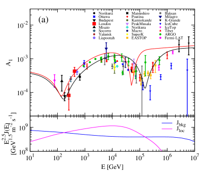
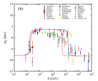
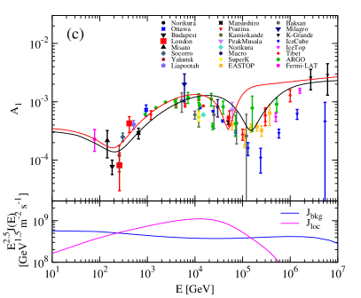
Fig. 1: The model calculations of the amplitude and phase of the dipole anisotropies, compared with the data. (a) and (b): The amplitude and phase for the case with alignment along the IBEX magnetic field. (c) and (d): The amplitude and phase for the case without alignment along the IBEX magnetic field. In each panel, the black curve is for all GCR species, and the red one is for protons. The bottom sub-panels of (a) and (c) show the streamings of all species from the background source (blue curve) and the nearby source (magenta curve).

Fig. 1 shows the calculated amplitudes and phases of the dipole anisotropies of GCRs in a wide energy range from 10 GeV to $>$PeV, compared with the measurements (Sakakibara et al., 1973; Gombosi et al., 1975; Bercovitch & Agrawal, 1981; Alexeyenko et al., 1981; Thambyahpillai, 1983; Nagashima et al., 1985; Swinson & Nagashima, 1985; Andreyev et al., 1987; Nagashima et al., 1989; Munakata et al., 1995; Mori et al., 1995; Fenton et al., 1995; Aglietta et al., 1995, 1996; Munakata et al., 1997; Ambrosio et al., 2003; Amenomori et al., 2005; Guillian et al., 2007; Aglietta et al., 2009; Alekseenko et al., 2009; Abdo et al., 2009; Abbasi et al., 2010, 2012; Aartsen et al., 2013; Bartoli et al., 2015; Amenomori et al., 2017; Bartoli et al., 2018; Ajello et al., 2019). The measurements made by the Fermi satellite are for protons (Ajello et al., 2019), while the other measurements by underground muon detectors and ground-based air shower detectors are for all particle species in GCRs. Therefore, in each plot we show the results for protons (red) and all species (black) individually. As can be expected from the model, two phase reversals should be observed in the anisotropies, at energies when the GCR streaming from the nearby source becomes dominant ($E\sim 100$ GeV) and sub-dominant ($E\sim 100$ TeV) compared with the background streaming. The competition of the two particle streamings leaves also imprints on the amplitudes, characterized by two dip-like structures at corresponding energies. These features are largely consistent with the measurements.

The local large-scale magnetic field may have a sizeable impact on the observed phases of anisotropies. Panels (c) and (d) of Fig. 1 give the results without the alignment along the IBEX magnetic field. The dips of the amplitudes become less distinct, because the two streamings from the background and the nearby source are not in the exactly opposite directions. After the projection along the magnetic field, they tend to cancel with each other at specific energies, resulting in deeper dips. Even bigger effects can be seen for the phases. Without considering the alignment effect due to the magnetic field, the anisotropy phases are determined solely by the source distributions. Therefore, for both low ($\lesssim 100$ GeV) and high ($\gtrsim 100$ TeV) energies, the excesses should point to the GC direction with R.A.$\sim-6$ hr. For intermediate energies the excesses point to the direction of the assumed nearby source with R.A.$\sim 5.5$ hr. The anisotropic diffusion results in an alignment along the IBEX magnetic field, and the phases change to $\sim-8$ hr for low and high energies and $\sim 4$ hr for intermediate energies, which are more consistent with the data.

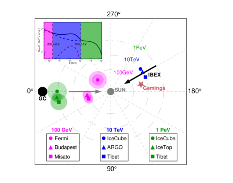
Fig. 2: The cartoon illustration of the co-evolution of spectra and anisotropies. This plot is a top-down view of the Milky Way from the Galactic north pole to the south pole, centering at the Sun. The black (grey) arrow shows the GCR streaming from the nearby (background) source. The dots, squares, and triangles show the observed excess directions of the anisotropies, with typical energies of 100 GeV (magenta), 10 TeV (blue), and 1 PeV (green), respectively. The directions of the GC, the Geminga SNR, and the IBEX magnetic field are also labelled. The inserted plot illustrates the structures of GCR spectra in this model, with three energy bands being shown by three colors.

4 CONCLUSION

In this work, we propose a simple two-component model to simultaneously explain the spectral features of GCR nuclei (including the hardening aroung $200$ GV and softening around $10$ TV), the amplitudes and two phase reversals of the dipole anisotropies. The energy spectra and anisotropies can thus be understood as the scalar and vector parts of this model, and a unified understanding of their complicated observational properties can be achieved in this two-component scenario. The algebraic sum of the fluxes of the background sources and the nearby source results in spectral hardenings around $O(200)$ GV and softenings around $O(10)$ TV rigidities, while the vector sum of the streamings gives the phase reversals and amplitude variations of the anisotropies. Fig. 2 shows a schematic illustration of the co-evolution of the energy spectra and anisotropies of GCRs. We note that, the anisotropy phases are more sensitive to reveal different components of GCRs than the spectra, due to the vector sum nature.

While this model can explain the overall observed results of the spectra and large-scale anisotropies, we note that the two-dimensional anisotropies may not be perfectly reproduced by this simple model. As expected by the model, for $E\lesssim 100$ GeV, the dipole anisotropies should be dominated by the background source component, which should be aligned to the (anti-)direction of the IBEX magnetic field (R.A.$\sim-9$ hr, Decl.$\sim 21^{\circ}$). However, the Fermi measurements showed that the two-dimensional anisotropy excess points to R.A.$=-9.7\pm 1.5$ hr, Decl.$=-51^{\circ}\pm 21^{\circ}$. The R.A. of the dipole anisotropy is well consistent with the model prediction, while the declination shows a deviation by about $3\sigma$. The significance of the Fermi observation is not high enough. Better measurements by future experiments like DAMPE (Chang et al., 2017) and HERD (Zhang et al., 2014) are necessary to further understand whether there is a discrepancy between the model and the data. The two-dimension anisotropy measurements for groundbased experiments are subject to difficulties of the absolute efficiency calibration, and are thus difficult for precise model tests.

The measurements of a few underground muon detectors were ambiguous. Measurements at different time showed variations of the anisotropy patterns for the muon detectors, such as London and Socorro (Speller et al., 1972; Swinson, 1974). In Fig. 1 we show the average sidereal component of the anisotropies measured by the muon detectors. Several models were proposed to understand the origin of such variations, such as the Jupiter’s magnetosphere (Swinson, 1974), the polarity reversal of the solar magnetic field (Cini-Castagnoli et al., 1975), or a variable asymmetric anisotropy component in the northern hemisphere which might be of solar origin (Nagashima et al., 1972, 1983). Observational evidence against those proposals also appeared (Jacklyn & Cini-Castagnoli, 1974; Nagashima & Tatsuoka, 1984; Nagashima et al., 1985; Swinson & Nagashima, 1985), and no consensus has been reached yet. We note that, in our model, the anisotropy patterns in the $O(100)$ GeV energy range are sensitive to the energy scales of the experiments, as shown in Fig. 1. The median energy of muon detectors might vary with time, due to the instrument calibration and/or the solar modulation. In addition, the energy resolution of those detectors is relatively poor. It is possible that the variations of the anistropy phases were due to the variations of median energies of different samples. Future direct detection experiments may test this hypothesis with more precise measurements in the low-energy band.

The second phase reversal around 100 TeV is also not well measured by current experiments. It is difficult to see at which energy the phase starts to reverse and how it changes from one phase to the other. Current indirect detection experiments are subject to large uncertainties of the composition discrimination, and the anisotropies are for mixed GCRs of all nuclei species. For energies above 100 TeV, it is also not clear whether the GCR anisotropy phase is closer to the GC or still aligned along the local magnetic field. We expect that improved measurements of the anisotropies of various mass groups by e.g., LHAASO (Cao et al., 2019) can be very helpful in testing our model and understanding the origin of GCR anisotropies.

The idea of this work may further apply to the energy spectra and anisotropies of cosmic rays at even higher energies, where the transition from Galactic to extragalactic origins occurs. The Pierre Auger Observatory reported the measurements of the anisotropies above 8 EeV, with direction of R.A.$\sim 6.7\pm 0.7$ hr and Decl.$=-24^{+12\circ}_{-13}$, which differs significantly from the GC but may be consistent with the infrared galaxy distribution after correcting the Galactic magnetic field effect on the anisotropies (Pierre Auger Collaboration et al., 2017). Improved measurements of how the anisotropies evolve between PeV and EeV energies may be used to diagnose the Galactic-extragalactic transition of cosmic rays.

References

- Aartsen et al. (2013) Aartsen, M. G., Abbasi, R., Abdou, Y., et al. 2013, ApJ, 765, 55
- Aartsen et al. (2016) Aartsen, M. G., Abraham, K., Ackermann, M., et al. 2016, ApJ, 826, 220
- Abbasi et al. (2010) Abbasi, R., Abdou, Y., Abu-Zayyad, T., et al. 2010, ApJ, 718, L194
- Abbasi et al. (2011) —. 2011, ApJ, 740, 16
- Abbasi et al. (2012) —. 2012, ApJ, 746, 33
- Abdo et al. (2008) Abdo, A. A., Allen, B., Aune, T., et al. 2008, Physical Review Letters, 101, 221101
- Abdo et al. (2009) Abdo, A. A., Allen, B. T., Aune, T., et al. 2009, ApJ, 698, 2121
- Abeysekara et al. (2014) Abeysekara, A. U., Alfaro, R., Alvarez, C., et al. 2014, ApJ, 796, 108
- Abeysekara et al. (2017) Abeysekara, A. U., Albert, A., Alfaro, R., et al. 2017, Science, 358, 911
- Abeysekara et al. (2019) Abeysekara, A. U., Alfaro, R., Alvarez, C., et al. 2019, ApJ, 871, 96
- Acero et al. (2016) Acero, F., Ackermann, M., Ajello, M., et al. 2016, ApJS, 223, 26
- Aglietta et al. (1995) Aglietta, M., Alessandro, B., Antonioli, P., et al. 1995, in International Cosmic Ray Conference, Vol. 2, International Cosmic Ray Conference, 800
- Aglietta et al. (1996) Aglietta, M., Alessandro, B., Antonioli, P., et al. 1996, ApJ, 470, 501
- Aglietta et al. (2009) Aglietta, M., Alekseenko, V. V., Alessandro, B., et al. 2009, ApJ, 692, L130
- Aguilar et al. (2015a) Aguilar, M., Aisa, D., Alpat, B., et al. 2015a, Phys. Rev. Lett., 115, 211101
- Aguilar et al. (2015b) —. 2015b, Phys. Rev. Lett., 114, 171103
- Aharonian et al. (2021) Aharonian, F., An, Q., Axikegu, Bai, L. X., et al. 2021, Phys. Rev. Lett., 126, 241103
- Ahlers (2016) Ahlers, M. 2016, Physical Review Letters, 117, 151103
- Ahlers & Mertsch (2017) Ahlers, M., & Mertsch, P. 2017, Progress in Particle and Nuclear Physics, 94, 184
- Ajello et al. (2019) Ajello, M., Baldini, L., Barbiellini, G., et al. 2019, ApJ, 883, 33
- Alekseenko et al. (2009) Alekseenko, V. V., Cherniaev, A. B., Djappuev, D. D., et al. 2009, Nuclear Physics B Proceedings Supplements, 196, 179
- Alemanno et al. (2021) Alemanno, F., An, Q., Azzarello, P., et al. 2021, Phys. Rev. Lett., 126, 201102
- Alexeyenko et al. (1981) Alexeyenko, V. V., Chudakov, A. E., Gulieva, E. N., & Sborschikov, V. G. 1981, in International Cosmic Ray Conference, Vol. 2, International Cosmic Ray Conference, 146
- Ambrosio et al. (2003) Ambrosio, M., Antolini, R., Baldini, A., et al. 2003, Phys. Rev. D, 67, 042002
- Amenomori et al. (2005) Amenomori, M., Ayabe, S., Cui, S. W., et al. 2005, ApJ, 626, L29
- Amenomori et al. (2006) Amenomori, M., Ayabe, S., Bi, X. J., et al. 2006, Science, 314, 439
- Amenomori et al. (2010) Amenomori, M., Bi, X. J., Chen, D., et al. 2010, ApJ, 711, 119
- Amenomori et al. (2017) —. 2017, ApJ, 836, 153
- An et al. (2019) An, Q., Asfandiyarov, R., Azzarello, P., et al. 2019, Science Advances, 5, eaax3793
- Andreyev et al. (1987) Andreyev, Y. M., Chudakov, A. E., Kozyarivsky, V. A., et al. 1987, in International Cosmic Ray Conference, Vol. 2, International Cosmic Ray Conference, 22
- Bartoli et al. (2013) Bartoli, B., Bernardini, P., Bi, X. J., et al. 2013, Phys. Rev. D, 88, 082001
- Bartoli et al. (2015) —. 2015, ApJ, 809, 90
- Bartoli et al. (2018) —. 2018, ApJ, 861, 93
- Bercovitch & Agrawal (1981) Bercovitch, M., & Agrawal, S. P. 1981, in International Cosmic Ray Conference, Vol. 10, International Cosmic Ray Conference, 246–249
- Binns et al. (2016) Binns, W. R., Israel, M. H., Christian, E. R., et al. 2016, Science, 352, 677
- Blasi (2013) Blasi, P. 2013, Astron. Astrophys. Rev., 21, 70
- Blasi & Amato (2012) Blasi, P., & Amato, E. 2012, J. Cosmology Astropart. Phys, 1, 011
- Blasi et al. (2012) Blasi, P., Amato, E., & Serpico, P. D. 2012, Phys. Rev. Lett., 109, 061101
- Bouyahiaoui et al. (2020) Bouyahiaoui, M., Kachelrieß, M., & Semikoz, D. V. 2020, Phys. Rev. D, 101, 123023
- Cao et al. (2019) Cao, Z., della Volpe, D., Liu, S., et al. 2019, arXiv e-prints, arXiv:1905.02773
- Cerri et al. (2017) Cerri, S. S., Gaggero, D., Vittino, A., Evoli, C., & Grasso, D. 2017, J. Cosmology Astropart. Phys, 10, 019
- Chang et al. (2017) Chang, J., Ambrosi, G., An, Q., et al. 2017, Astroparticle Physics, 95, 6
- Cini-Castagnoli et al. (1975) Cini-Castagnoli, G., Marocchi, D., Elliot, H., Marsden, R. G., & Thambyahpillai, T. 1975, in International Cosmic Ray Conference, Vol. 4, International Cosmic Ray Conference, 1453
- Erlykin & Wolfendale (2006) Erlykin, A. D., & Wolfendale, A. W. 2006, Astroparticle Physics, 25, 183
- Evoli et al. (2017) Evoli, C., Gaggero, D., Vittino, A., et al. 2017, J. Cosmology Astropart. Phys, 2, 015
- Faherty et al. (2007) Faherty, J., Walter, F. M., & Anderson, J. 2007, Ap&SS, 308, 225
- Fenton et al. (1995) Fenton, K. B., Fenton, A. G., & Humble, J. E. 1995, in International Cosmic Ray Conference, Vol. 4, International Cosmic Ray Conference, 635
- Giacinti et al. (2018) Giacinti, G., Kachelrieß, M., & Semikoz, D. V. 2018, J. Cosmology Astropart. Phys, 2018, 051
- Gombosi et al. (1975) Gombosi, T., Kóta, J., Somogyi, A. J., et al. 1975, in International Cosmic Ray Conference, Vol. 2, International Cosmic Ray Conference, 586–591
- Grenier et al. (2015) Grenier, I. A., Black, J. H., & Strong, A. W. 2015, ARA&A, 53, 199
- Guillian et al. (2007) Guillian, G., Hosaka, J., Ishihara, K., et al. 2007, Phys. Rev. D, 75, 062003
- Guo et al. (2016) Guo, Y.-Q., Tian, Z., & Jin, C. 2016, ApJ, 819, 54
- Jacklyn & Cini-Castagnoli (1974) Jacklyn, R. M., & Cini-Castagnoli, G. 1974, PASA, 2, 293
- Kachelrieß et al. (2015) Kachelrieß, M., Neronov, A., & Semikoz, D. V. 2015, Phys. Rev. Lett., 115, 181103
- Kumar & Eichler (2014) Kumar, R., & Eichler, D. 2014, ApJ, 785, 129
- Liu et al. (2019) Liu, W., Guo, Y.-Q., & Yuan, Q. 2019, J. Cosmology Astropart. Phys, 2019, 010
- Luo et al. (2022) Luo, Q., Qiao, B.-q., Liu, W., Cui, S.-w., & Guo, Y.-q. 2022, ApJ, 930, 82
- Manchester et al. (2005) Manchester, R. N., Hobbs, G. B., Teoh, A., & Hobbs, M. 2005, AJ, 129, 1993
- Mertsch & Funk (2015) Mertsch, P., & Funk, S. 2015, Physical Review Letters, 114, 021101
- Mori et al. (1995) Mori, S., Yasue, S., Munakata, K., et al. 1995, in International Cosmic Ray Conference, Vol. 4, International Cosmic Ray Conference, 648
- Munakata et al. (1995) Munakata, K., Yasue, S., Mori, S., et al. 1995, in International Cosmic Ray Conference, Vol. 4, International Cosmic Ray Conference, 639
- Munakata et al. (1997) Munakata, K., Kiuchi, T., Yasue, S., et al. 1997, Phys. Rev. D, 56, 23
- Nagashima et al. (1972) Nagashima, K., Fujimoto, K., Fujii, Z., Ueno, H., & Kondo, I. 1972, Rep. Ionos. Space Res. Jpn, 26, 31
- Nagashima et al. (1989) Nagashima, K., Fujimoto, K., Sakakibara, S., et al. 1989, Nuovo Cimento C Geophysics Space Physics C, 12, 695
- Nagashima et al. (1985) Nagashima, K., Sakakibara, S., Fenton, A. G., & Humble, J. E. 1985, Planet. Space Sci., 33, 395
- Nagashima & Tatsuoka (1984) Nagashima, K., & Tatsuoka, R. 1984, Nuovo Cimento C Geophysics Space Physics C, 7, 379
- Nagashima et al. (1983) Nagashima, K., Tatsuoka, R., & Matsuzaki, S. 1983, Nuovo Cimento C Geophysics Space Physics C, 6C, 550
- Pierre Auger Collaboration et al. (2017) Pierre Auger Collaboration, Aab, A., Abreu, P., et al. 2017, Science, 357, 1266
- Pohl & Eichler (2013) Pohl, M., & Eichler, D. 2013, ApJ, 766, 4
- Qiao et al. (2019) Qiao, B.-Q., Liu, W., Guo, Y.-Q., & Yuan, Q. 2019, J. Cosmology Astropart. Phys, 2019, 007
- Recchia et al. (2016) Recchia, S., Blasi, P., & Morlino, G. 2016, MNRAS, 462, L88
- Sakakibara et al. (1973) Sakakibara, S., Ueno, H., Fujimoto, K., Kondo, I., & Nagashima, K. 1973, in International Cosmic Ray Conference, Vol. 2, International Cosmic Ray Conference, 1058
- Savchenko et al. (2015) Savchenko, V., Kachelrieß, M., & Semikoz, D. V. 2015, ApJ, 809, L23
- Schwadron et al. (2014) Schwadron, N. A., Adams, F. C., Christian, E. R., et al. 2014, Science, 343, 988
- Seo & Ptuskin (1994) Seo, E. S., & Ptuskin, V. S. 1994, ApJ, 431, 705
- Smith et al. (1994) Smith, V. V., Cunha, K., & Plez, B. 1994, A&A, 281, L41
- Speller et al. (1972) Speller, R., Thambyahpillai, T., & Elliot, H. 1972, Nature, 235, 25
- Strong et al. (2007) Strong, A. W., Moskalenko, I. V., & Ptuskin, V. S. 2007, Annual Review of Nuclear and Particle Science, 57, 285
- Sveshnikova et al. (2013) Sveshnikova, L. G., Strelnikova, O. N., & Ptuskin, V. S. 2013, Astroparticle Physics, 50, 33
- Swinson (1974) Swinson, D. B. 1974, J. Geophys. Res., 79, 3695
- Swinson & Nagashima (1985) Swinson, D. B., & Nagashima, K. 1985, Planet. Space Sci., 33, 1069
- Thambyahpillai (1983) Thambyahpillai, T. 1983, in International Cosmic Ray Conference, Vol. 3, International Cosmic Ray Conference, 383
- Tomassetti (2012) Tomassetti, N. 2012, ApJ, 752, L13
- Wallner et al. (2016) Wallner, A., Feige, J., Kinoshita, N., et al. 2016, Nature, 532, 69
- Yang et al. (2016) Yang, R., Aharonian, F., & Evoli, C. 2016, Phys. Rev. D, 93, 123007
- Zhang et al. (2021) Zhang, P.-P., Qiao, B.-Q., Liu, W., et al. 2021, J. Cosmology Astropart. Phys, 2021, 012
- Zhang et al. (2014) Zhang, S. N., Adriani, O., Albergo, S., et al. 2014, in Proc. SPIE, Vol. 9144, 91440X