An Improved Reinforcement Learning Algorithm for Learning to Branch

Abstract

Most combinatorial optimization problems can be formulated as mixed integer linear programming (MILP), in which branch-and-bound (B&B) is a general and widely used method. Recently, learning to branch has become a hot research topic in the intersection of machine learning and combinatorial optimization. In this paper, we propose a novel reinforcement learning-based B&B algorithm. Similar to offline reinforcement learning, we initially train on the demonstration data to accelerate learning massively. With the improvement of the training effect, the agent starts to interact with the environment with its learned policy gradually. It is critical to improve the performance of the algorithm by determining the mixing ratio between demonstration and self-generated data. Thus, we propose a prioritized storage mechanism to control this ratio automatically. In order to improve the robustness of the training process, a superior network is additionally introduced based on Double DQN, which always serves as a Q-network with competitive performance. We evaluate the performance of the proposed algorithm over three public research benchmarks and compare it against strong baselines, including three classical heuristics and one state-of-the-art imitation learning-based branching algorithm. The results show that the proposed algorithm achieves the best performance among compared algorithms and possesses the potential to improve B&B algorithm performance continuously.

1 Introduction

The mixed integer linear programming (MILP) is one of the most widely-used mathematical formulations in practical scenarios of optimization, such as planning and scheduling, bin packing, resource allocation, etc. Generally, the vast majority of MILP problems are NP-hard, which makes it inevitable to compromise in terms of solving speed, precision, generalization, etc. when using traditional methods to solve them. The NP-hardness is mainly due to the scale, such as the number of integer variable. Therefore, some scholars pay attention to improving the solutions of MILP by adopting some machine learning algorithms such as the imitation learning, reinforcement learning, etc. Huang et al. (2021). The branch-and-bound (B&B) algorithm, together with the various skills for increasing its efficiency, constitute one of the cores of MILP. B&B algorithm enumerates the candidate solutions systematically by means of state space search, in which the set of candidates solutions is considered to form a search tree with the full set at the root. The efficiency of B&B algorithm mainly depends on branching variable selection and node selection. In this paper, we concentrate on the former. Usually, choosing good variables to branch on can lead to a dramatic reduction in terms of the number of nodes needed to solve an instance Alvarez et al. (2014a).

At present, there is still no commonly accepted method for the strategy of branching variable selection. Traditional methods are mostly simple heuristic rules, such as the Most Infeasible branching, Pseudo-Cost branching (PC), Strong Branching (SB), Hybrid Strong/Pseudocost Branching, Pseudocost branching with strong branching initialization, Reliability Branching (RB), etc. Achterberg et al. (2005), in which PC and SB approaches are the two most common heuristic rules. PC is a sophisticated rule in the sense that it keeps a history of the success of the variables on which already has been branched Benichou et al. (1971). Despite tiny computation, PC relies on human intuition and extensive engineering, requiring significant manual tuning. SB is to evaluate which of the fractional candidates gives the largest progress before actually branching on any of them Applegate et al. (1995). This approach can lead to the smallest search tree currently known. However, it increases the computation significantly.

Alvarez et al. (2014a) adopted machine learning algorithms early to learn the strategies of branching variable selection in the B&B algorithm. Such kind of learning-based strategies are also known as learning to branch. Learning to branch is different from the traditional optimization methods. It introduces the concept of learning in the optimization process to help search the optimal solution more effectively. Balcan et al. (2018) has shown empirically and theoretically that it is possible to learn high-performing branching strategies for a given application domain. Learning branching policies for MILP has become an active research area. Most relevant researches use supervised or imitation learning to imitate SB method and specialize it to distinct classes of problems. However, only the data collected by expert policies can be used to train during the imitation learning process in their studies, which leads to mismatch between training data and real-world data. This factor prevents learning a good enough policy by the means of imitation learning. Some other scholars attempt to use reinforcement learning and model the variable selection process as a Markov Decision Process (MDP), to obtain more effective and non-myopic policies. However, for each instance, the MDP contains a large number of steps and actions, which can lead to a large variance in gradient estimation. Besides, too large action set makes it hard to explore in MILP. These challenges restrict the applications of reinforcement learning in solving MILP Sun et al. (2020).

In this work, we attempt to address the above challenges by proposing a novel reinforcement learning-based branching algorithm. Although there have been some ideas to solve the branching problem by means of reinforcement learning Sun et al. (2020), we propose to address the learning problem in a novel way, of which the contributions are summarized as the following points:

• Demonstration data is leveraged to accelerate the learning massively at the early stage. With the improvement of the training effect, the agent starts to interact with the environment with its learned policy gradually.

• The RL agent updates its network with a mixture of demonstration and self-generated data. We introduce a prioritized storage mechanism to control the mixing ratio automatically.

• In order to improve the robustness of the training process, a superior Q-network is additionally introduced based on Double DQN, which always serves as a Q-network with competitive performance.

• We evaluate the performance of the proposed algorithm on three benchmarks with comparative experiments against three heuristic approaches and one state-of-the-art (SOTA) imitation learning-based branching algorithm  Gasse et al. (2019). With the dual integral as a metric, our algorithm outperforms the SOTA imitation learning-based branching algorithm by 35.88% at most. Besides, we also make an ablation study to validate the rationality of this algorithm.

2 Related work

Supervised machine learning and imitation learning are currently the mainstream approaches for learning to branch.  Alvarez et al. (2014b) proposed a new approach that uses supervised learning to improve the performances of optimization algorithms in the context of MILP.  Khalil et al. (2016) proposed a machine learning framework for variable branching in MILP. Based on the data collected by SB method, they learned an easy-to-evaluate surrogate function that mimics the SB method, by means of solving a learning-to-rank problem. And it is competitive with a state-of-the-art commercial solver.  Gasse et al. (2019) proposed a new graph convolutional neural network (GCNN) model for learning to branch, which leverages the natural variable-constraint bipartite graph representation of MILP. They trained the GCNN model via imitation learning from the SB method, and demonstrated that this model produced policies that improved upon state-of-the-art machine learning methods for branching.  Gupta et al. (2020) proposed a new hybrid architecture for efficient branching on CPU machines, which combined the expressive power of GCNNs with computationally inexpensive multi-layer perceptrons (MLPs) for branching.

In order to obtain more efficient and non-myopic policies, some scholars attempt to use reinforcement learning to solve this problem.  Etheve et al. (2020) proposed Fitting for Minimising the SubTree Size, a novel approach based on reinforcement learning, whose strength lies in the consistency between a local value function and a global metric of interest.  Sun et al. (2020) introduced a novel set representation and optimal transport distance for the branching process associated with a policy, to train the reinforcement learning agent. The results showed substantial improvements in empirical evaluation. More related researches can refer to the survey provided by  Huang et al. (2021).

3 Background

3.1 Mixed integer linear programs

A mixed integer linear program is an optimization problem of the form

$$\mathop{\arg\min}\limits_{\textbf{x}}\left\{\textbf{c}^{T}\textbf{x}\mid\textbf{Ax}\leq\textbf{b},\textbf{l}\leq\textbf{x}\leq\textbf{u},\textbf{x}\in\mathbb{Z}^{\textit{p}}\times\mathbb{R}^{\textit{n-p}}\right\}$$

where $\textbf{c}\in\mathbb{R}^{\textit{n}}$ is the objective coefficient vector, $\textbf{A}\in\mathbb{R}^{\textit{m}\times\textit{n}}$ is the constraint coefficient matrix, $\textbf{b}\in\mathbb{R}^{\textit{m}}$ is the constraint right-hand-side vector, $\textbf{l},\textbf{u}\in\mathbb{R}^{\textit{n}}$ represent the lower and upper variable bound vectors respectively, and p is the number of integer variables. The linear programming (LP) relaxation of a MILP is shown below

$$\mathop{\arg\min}\limits_{\textbf{x}}\left\{\textbf{c}^{T}\textbf{x}\mid\textbf{Ax}\leq\textbf{b},\textbf{l}\leq\textbf{x}\leq\textbf{u},\textbf{x}\in\mathbb{R}^{\textit{n}}\right\}$$

The LP solution provides a lower bound to the original MILP. Specifically, if the LP solution is subject to the integer constraint, then it is also a optimal feasible solution of the MILP. Otherwise, the LP relaxation is required to be decomposed into two sub-problems. This is done by branching on a variable that does not obey the integrality constraint in the current LP solution. The solving process terminates when the feasible regions cannot be decomposed anymore, and subsequently a certificate of optimality or infeasibility can be provided respectively.

3.2 Branch-and-bound

A key factor influencing the efficiency of B&B algorithm is how to select a fractional variable to branch on. There are commonly two basic heuristic branching rules, including Strong Branching (SB) and Pseudocost Branching (PC) strategies. Most other heuristic rules are derived from them. The details of SB and PC are described as follows.

SB is to evaluate which of the fractional candidates gives the best progress before actually branching on any of them. For each candidate variable, this evaluation process is realized by solving the LP relaxations of the two sub-problems. Thus, a huge amount of computation is required when adopting SB method.

PC is a sophisticated rule in the sense that it keeps a history of the success of the variable on which already has been branched. $\Psi_{j}^{+}$ ($\Psi_{j}^{-}$) denotes the average unit objective gain taken over upwards (downwards) branching on $x_{j}$ in previous nodes. Pseudocost branching at node N with LP relaxation solution $\check{x}$ consists in computing values:

$$PC_{j}=score((\check{x}_{j}-\left\lfloor\check{x}_{j}\right\rfloor)\Psi_{j}^{-},(\left\lceil\check{x}_{j}\right\rceil-\check{x}_{j})\Psi_{j}^{+})$$

and choosing the candidate variable with highest such value. Compared with the SB method, PC method is simpler but faster. However, PC method is overly dependent on human intuition and extensive engineering, requiring considerable manual tuning.

3.3 Reinforcement learning for branching

According to the reference Gasse et al. (2019), the B&B process can be modeled as a Markov decision process (MDP), in which the solver is considered as the environment. Prouvost et al. presented Ecole, a new library to simplify machine learning research for combinatorial optimization, which lowers the bar of entry and accelerates innovation in this field Prouvost et al. (2020).

Based on Ecole, the B&B is episodic. Each episode corresponds to a MILP instance. The state and reward of the MDP can be defined by an observation function and a reward function in Ecole respectively. Or even users can define new environments and simply reuse existing observation and reward functions to fulfill specific requirements. The probability of a trajectory $\tau=(s_{0},...,s_{T})\in T$ depends on both the branching policy $\pi$ and the remaining components of the solver,

$$p_{\pi}(\tau)=p(s_{0})\prod_{t=0}^{T-1}\sum_{a\in A(s_{t})}\pi(a\mid s_{t})p(s_{t+1}\mid s_{t},a)$$

Compared with the imitation learning, the reinforcement learning can balance the exploration and exploitation in an unknown environment. Theoretically speaking, it possesses higher performance.

4 Proposed algorithm

In this paper, a novel algorithm based on reinforcement learning is proposed for dealing with the B&B variable selection problem in MILP. In order to illustrate our algorithm, we organize this section in two parts. Firstly, we give our formulation of the variable selection process as a reinforcement learning problem. Then, we introduce the specific implementation of this algorithm in detail.

4.1 Formulation

Let the solver be the environment. The sequential decision making of variable selection can be formulated as a Markov Decision Process (MDP). Specifically, the state s, action space A, action a, transition P, and reward r are described as follows.

• State: A node bipartite graph representation of B&B states used in Gasse et al. Gasse et al. (2019), using the ecole.observation.NodeBipartite observation function Prouvost et al. (2020).

• Action space: The set of candidate variables.

• Action: The selected candidate variable to branch on.

• Transition: Given state $s_{t}$ and action $a_{t}$, the next state $s_{t+1}$ is determined by the node selection policy.

• Reward: The reward is defined as the dual integral since the previous state, where the integral is computed with respect to the solving time. Details are explained in the Metric part of the Experimental evaluation section.

• Next state: The node bipartite graph representation of the next node.

• Next action space: The set of candidate variables corresponding to the next node.

• Done: The termination flag.

4.2 Algorithm

In this section, based on Double DQN Van Hasselt et al. (2016), we propose a novel deep reinforcement learning algorithm for branching problem. It leverages demonstration data to massively accelerate the learning process by means of offline reinforcement learning. In order to balance the exploration and exploitation, this algorithm can automatically control the mixing ratio of demonstration data during the learning process due to a prioritized storage mechanism. Besides, in order to avoid the multi-fold challenges caused by the large state space and action set, we additionally introduce a superior network, which always serves as a Q-network with competitive performance. Figure 1 shows an overview of the proposed algorithm.

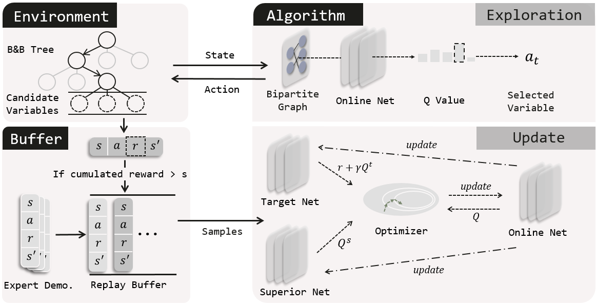
Figure 1: An overview of the proposed algorithm: Environment corresponds to a solver aiming at variable selection problem in B&B; Buffer is filled with both demonstration and self-generated data, and only high-quality self-generated data can be added in it; The main part of the algorithm is composed of three networks, where online net is used for action selection, target net is used for action evaluation to decompose the max operation, superior net always serves as a Q-network with competitive performance to help to stabilize the training process.

In order to accelerate the learning process at the early stage, the replay buffer is given a set of demonstration data, which will remain permanently. In this phase, the agent trains solely on the demonstration data by means of offline reinforcement learning, without any interaction with the environment. And it can obtain relatively good performance in a short period of time. However, the agent may make incorrect estimates for unfamiliar $(s,a)$ pairs due to the lack of interaction with the environment. Therefore, we introduce a prioritized storage mechanism, in which the agent collects self-generated data and adds it to the replay buffer conditionally. In detail, only the data collected by the policy that leads to high performance is added to the replay buffer, which can prevent some poor-quality data from misleading the training. Data is added to the buffer until it is full, and then agent starts overwriting old data in the buffer. However, the agent never overwrites the demonstration data. In this way, the mixing ratio between demonstration and self-generated data can be controlled automatically.

It is commonly believed that too large action set increases the difficulty of RL training Sun et al. (2020). The RL agent may learn a local optimal policy, or even worse, a random policy. In order to solve this issue, a superior Q-network is additionally introduced based on the framework of Double DQN. And then, there are three Q-networks in this frame, i.e. online network, target network, and superior network. The online network is used for action selection. The target network is used for action evaluation to decompose the max operation. The superior network always serves as a Q-network with competitive performance to help to stabilize the training process. Similar to the works of Gasse et al., a graph convolutional neural network (GCNN) is adopted to parametrize the Q-network Gasse et al. (2019). In detail, the input of the GCNN model is the bipartite state representation $s_{t}=(\mathcal{G},\textbf{C},\textbf{V},\textbf{E})$. The graph convolution can be broken down into two successive passes, one from variables to constraints and the other one from constraints to variables, which are shown as

$$c_{i} \leftarrow f_{c}(c_{i},\sum_{j}^{(i,j)\in\varepsilon}{g_{c}(c_{i},v_{j},e_{i,j})})$$

$$v_{i} \leftarrow f_{v}(v_{j},\sum_{j}^{(i,j)\in\varepsilon}{g_{v}(c_{i},v_{j},e_{i,j})})$$

where $f_{c}$, $f_{v}$, $g_{c}$ and $g_{v}$ are two-layer perceptrons with ReLU activation functions. In addition to TD loss used in Double DQN, we add another term in the overall loss used to update the online network, which is shown as

$$\mathcal{L}(\theta)= \mathbb{E}(r+\gamma\max_{a^{\prime}}Q^{t}(s^{\prime},a^{\prime},\theta^{t})-Q(s,a,\theta))$$

$$+ \mathbb{E}(Q^{s}(s,a,\theta^{s})-Q(s,a,\theta))$$

where the superscript t and s represent target and superior respectively.

Pseudo-code is sketched in Algorithm 1. The behavior policy $\pi^{\varepsilon Q_{\theta}}$ is $\varepsilon$-greedy with respect to $Q_{\theta}$.

Algorithm 1 Double Deep Q-learning with Superior Network

0:  $D^{replay}$: initialized with demonstration data set;  $\theta$: weights for online network (random initialization);  $\theta^{t}$: weights for target network (random initialization);  $\theta^{s}$: weights for superior network (random initialization);  $\tau^{t}$: frequency at which to update target network;  $\tau^{s}$: frequency at which to evaluate the trained policy;  $G_{0}$: a threshold to measure the performance of behavior policy;  $G_{best}$: the cumulative reward of the best trained policy in the training process (zero initialization).

1:  for steps $t\in{1,2,...}$ do

2:     Sample action from behavior policy $a\sim\pi^{\varepsilon Q_{\theta}}$

3:     Play action a and observe $(s^{\prime},r)$

4:     Store $(s,a,r,s^{\prime})$ into a temporary buffer $D^{temporary}$

5:     Sample a mini-batch of n transitions from $D^{replay}$

6:     Calculate loss $\mathcal{L}$ using target and superior network

7:     Perform a gradient descent step to update $\theta$

8:     if $t\mod\tau^{t}=0$ then

9:        $\theta^{t}\leftarrow\theta$

10:     end if

11:     if $t\mod\tau^{s}=0$ then

12:        Compute the cumulative reward G to evaluate the trained policy

13:        if $G>G_{0}$ then

14:           Store $(s,a,r,s^{\prime})$ in $D^{temporary}$ into $D^{replay}$, overwriting oldest self-generated transition if over capacity, emptying $D^{temporary}$

15:        end if

16:        if $G>G_{best}$ then

17:           $\theta^{s}\leftarrow\theta$

18:        end if

19:     end if

20:     $s\leftarrow s^{\prime}$

21:  end for

5 Experimental evaluation

In this part, we achieve a comparative experiment against three heuristic approaches and one machine learning approach to evaluate the effectiveness of our algorithm. Meanwhile, we also make an ablation study to validate the rationality of this algorithm.

5.1 Setup

The proposed method is trained on a computing server which is equipped with Intel(R) Xeon(R) Platinum 8180M CPU@2.50GHz, a V100 GPU card with 32GB graphic memory and 1TB main memory.

Benchmark: We evaluate our algorithm on three benchmarks from diverse application areas, including Balanced Item Placement (BIP), Workload Apportionment (WA), and an Anonymous Problem (AP). All the three benchmarks are from the Machine Learning for Combinatorial Optimization (ML4CO) NeurIPS 2021 competition NeurIPS 2021 Competition (2021). The first two benchmarks are inspired by real-life applications of large-scale systems at Google, and the third benchmark is an anonymous problem also inspired by a real-world, large-scale industrial application.

Metric: The dual integral is used as the evaluation metric, which measures the area over the curve of the solver’s dual bound (a.k.a. global lower bound). It usually corresponds to a solution of a valid relaxation of the MILP. Theoretically, a small dual integral will lead to both good and fast decisions. By branching, the LP relaxations corresponding to the branch-and-bound tree leaves get tightened, and the dual bound increases over time. With a time limit T, the dual integral expresses as:

$$Tc^{T}x^{*}-\int_{t=0}^{T}z_{t}^{*}dt$$

where $z_{t}^{*}$ is the best dual bound at time t, and $Tc^{T}x^{*}$ is an instance-specific constant that depends on the optimal solution value $c^{T}x^{*}$. The dual integral is to be minimized, and takes an optimal value of 0. The optimization process is shown in Figure 2. In the experiments of this paper, the time limit is set as 15 minutes.

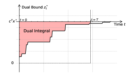
Figure 2: The dual integral during the optimization process

Baselines: We compete against three heuristic approaches, including strong branching, pseudocost branching, active constraint method (a method suitable for solving large-scale problems) Patel and Chinneck (2007), and one machine learning approach, i.e. imitation learning from the strong branching expert rule Gasse et al. (2019).

5.2 Comparative experiment

In this experiment, the demonstration data set size is 50K for BIP and AP datasets, and 10K for the WA dataset.

• Batch size: 32 for BIP and AP, 24 for WA

• Learning rate: 0.001

• $\varepsilon$-greedy with $\varepsilon=0.01$

• Dimension of input embedding in GCNN: 64

• Replay buffer size: 100K for BIP and AP, 20K for WA

• Discount factor: 0.99

• Period for target model’s hard update: $\tau^{t}$ = 500

• Period for evaluating the trained policy: $\tau^{s}$ = 1000

• Epochs: 50K

Algorithms	Scores	Wins
SB	3767.95	0/100
PC	4268.95	1/100
AC	5800.05	3/100
IL	5335.94	33/100
RL	7250.29	63/100

Table 1: Evaluation results on Balanced Item Placement

Algorithms	Scores	Wins
SB	623469.3	13/100
PC	624727.1	18/100
AC	624256.8	14/100
IL	624326.4	20/100
RL	624932.8	35/100

Table 2: Evaluation results on Workload Apportionment

Algorithms	Scores	Wins
SB	30387450	27/100
PC	31600684	1/100
AC	30995284	1/100
IL	32446178	29/100
RL	32547931	42/100

Table 3: Evaluation results on Anonymous Problem

We evaluate different branching algorithms on 100 instances for each benchmarks. Evaluation results on three benchmarks are shown in Tables 1-3 respectively.

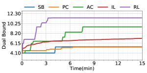
(a) Balanced Item Placement

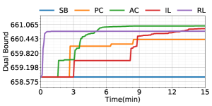
(b) Workload Apportionment

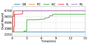
(c) Anonymous Problem

Figure 3: The dual bound curve of different algorithms during the solving process

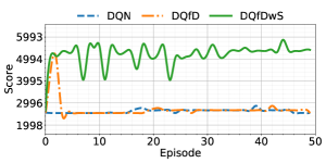
(a) Balanced Item Placement

(b) Workload Apportionment

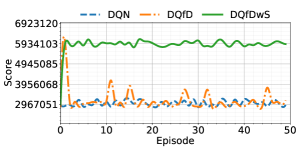
(c) Anonymous Problem

Figure 4: The performance curve of ablation study in the training process

In Tables 1-3, SB, PC, AC, IL, RL represent the strong branching, pseudocost branching, active constraint method, imitation learning from the strong branching expert rule, and our algorithm respectively.

As can be seen, AC is indeed more suitable for solving large-scale MILP problems among the three heuristic algorithms. However, its performance is still inferior to our algorithm. Furthermore, it is worth mentioning that both the imitation learning algorithm proposed by Gasse et al. and our reinforcement learning algorithm learn from the demonstration data collected by SB and PC approaches. It can be observed that both machine learning algorithms have a greater performance improvement than expert rules. Meanwhile, under the same conditions including the data set size, learning rate, etc, the performance of our algorithm is significantly better than that of the imitation learning algorithm, which is demonstrated by the facts that our algorithm obtains the highest scores and wins on the largest number of instances for all three benchmarks. Compared with IL, this proposed algorithm possesses a performance improvement of up to 35.88%, exactly on the first benchmark.

In order to further illustrate the effect of different algorithms, we perform branch and bound on one instance for each benchmark, and give the dual bound curve in this process, which are shown in Figure 3. It can be seen that our algorithm can indeed result in the smallest dual integral, which suggests that it can lead to both the best and fastest decisions.

5.3 Ablation study

We present an ablation study of our proposed algorithm by comparing with two reinforcement learning algorithms, including the deep reinforcement learning with double Q-learning and the double deep Q-learning only with demonstration data. We plot the performance curves of different algorithms on test dataset during training process for all three benchmarks. The results are shown in Figure 4. DQN, DQfD and DQfDwS represent the Double DQN, Double DQN with the guidance of expert rules and our algorithm respectively. It can be found that the performance of deep reinforcement learning with double Q-learning is extremely poor to solve the MILP problems, in which the trained policy are almost always random. After adding the guidance of expert rules, it can be seen that the training process is greatly accelerated in the early stage of training, but it will soon fall into the local optimal strategy, which is caused by the too large state space and action set. However, after adding the superior Q-network, our algorithm can not only help to accelerate the training process in the early stage but also help to stabilize the training process in the late stage. Thus our algorithm has the potential to advance the performance of B&B algorithm continuously.

6 Conclusion

In this paper, we propose a novel reinforcement learning method to improve the B&B algorithm performance in MILP. Firstly, in view of the shortcomings of reinforcement learning algorithms that are difficult to explore in the early stage of this problem, demonstration data collected by strong branch rule is leveraged to accelerate the learning process significantly. Subsequently, as the training effect improves, the agent gradually begins to interact with the solver with its learned policy. To avoid misleading training by low-quality self-generated data, a prioritized storage mechanism is introduced to guarantee the high quality of data in the replay buffer and control the mixing ratio of demonstration and self-generated data automatically. Besides, too large state space and action set lead to a large variance in gradient estimation, which makes it hard to explore in MILP. In order to address this challenge, we additionally introduced a superior Q-network based on Double DQN, which always serves as a Q-network with competitive performance. A group of comparative experiments and ablation studies demonstrate that this algorithm is significantly effective in performance improvement of B&B algorithm.

References

- Achterberg et al. [2005] Tobias Achterberg, Thorsten Koch, and Alexander Martin. Branching rules revisited. Operations Research Letters, 33(1):42–54, Jan 2005.
- Alvarez et al. [2014a] Alejandro Marcos Alvarez, Quentin Louveaux, and Louis Wehenkel. A supervised machine learning approach to variable branching in branch-and-bound. In IN ECML, 2014.
- Alvarez et al. [2014b] Marcos Alvarez, Alejandro, Quentin Louveaux, and Louis Wehenkel. A supervised machine learning approach to variable branching in branch-and-bound. 2014.
- Applegate et al. [1995] D Applegate, R Bixby, V Chvátal, and W Cook. Finding cuts in the tsp. DIMACS Technical Report 95-05, Mar 1995.
- Balcan et al. [2018] MF Balcan, T Dick, T Sandholm, and E Vitercik. Learning to branch. In Proceedings of the 35th International Conference on Machine Learning, Stockholm, Sweden, July 2018. ACM.
- Benichou et al. [1971] M. Benichou, J. M. Gauthier, P. Girodet, G. Hentges, G. Ribiere, and O. Vincent. Experiments in mixed-integer linear programming. Mathematical Programming, 1:76–94, Dec 1971.
- Etheve et al. [2020] Marc Etheve, Zacharie Alès, Côme Bissuel, Olivier Juan, and Safia Kedad-Sidhoum. Reinforcement learning for variable selection in a branch and bound algorithm. In International Conference on Integration of Constraint Programming, Artificial Intelligence, and Operations Research, pages 176–185. Springer, 2020.
- Gasse et al. [2019] Maxime Gasse, Didier Chételat, Nicola Ferroni, Laurent Charlin, and Andrea Lodi. Exact combinatorial optimization with graph convolutional neural networks. arXiv preprint arXiv:1906.01629, 2019.
- Gupta et al. [2020] Prateek Gupta, Maxime Gasse, Elias B Khalil, M Pawan Kumar, Andrea Lodi, and Yoshua Bengio. Hybrid models for learning to branch. arXiv preprint arXiv:2006.15212, 2020.
- Huang et al. [2021] Lingying Huang, Xiaomeng Chen, Wei Huo, Jiazheng Wang, Fan Zhang, Bo Bai, and Ling Shi. Branch and bound in mixed integer linear programming problems: A survey of techniques and trends. arXiv preprint arXiv:2111.06257, 2021.
- Khalil et al. [2016] Elias Khalil, Pierre Le Bodic, Le Song, George Nemhauser, and Bistra Dilkina. Learning to branch in mixed integer programming. In Proceedings of the AAAI Conference on Artificial Intelligence, volume 30, 2016.
- NeurIPS 2021 Competition [2021] NeurIPS 2021 Competition. Machine learning for combinatorial optimization, https://www.ecole.ai/2021/ml4co-competition/,, 2021.
- Patel and Chinneck [2007] Jagat Patel and John W Chinneck. Active-constraint variable ordering for faster feasibility of mixed integer linear programs. Mathematical Programming, 110(3):445–474, 2007.
- Prouvost et al. [2020] Antoine Prouvost, Justin Dumouchelle, Lara Scavuzzo, Maxime Gasse, Didier Chételat, and Andrea Lodi. Ecole: A gym-like library for machine learning in combinatorial optimization solvers. arXiv preprint arXiv:2011.06069, 2020.
- Sun et al. [2020] Haoran Sun, Wenbo Chen, Hui Li, and Le Song. Improving learning to branch via reinforcement learning. 2020.
- Van Hasselt et al. [2016] Hado Van Hasselt, Arthur Guez, and David Silver. Deep reinforcement learning with double q-learning. In Proceedings of the AAAI conference on artificial intelligence, volume 30, 2016.