Analytic estimates of quasi-normal mode frequencies for
black holes in General Relativity and beyond

Abstract

In this chapter, we review the eikonal technique to analytically derive approximate quasi-normal mode frequencies of black holes. We first review the procedure in General Relativity and extend it to theories beyond General Relativity. As an example of the latter, we focus on scalar Gauss-Bonnet gravity in which a scalar field can couple to the Gauss-Bonnet invariant in an arbitrary way in the action. In this theory, metric and scalar perturbations are coupled in the polar sector, forcing the isospectrality to break and making the eikonal calculation more complex. We show that the analytic estimates can accurately capture the numerical behavior of the quasi-normal mode frequencies, especially when the coupling constant of the theory is small.

I Introduction

A post-merger signal of gravitational waves (GWs) from a black hole (BH) coalescence is characterized by a quasi-normal mode (QNM) ringdown Kokkotas and Schmidt (1999); Berti et al. (2009) (see the left panel of Fig. 1). Normal modes are a pattern of motion in which all parts of the system oscillate with the same frequency. For example, masses on springs will undergo normal mode oscillations if there is no friction. On the other hand, QNMs are normal modes with damping in a dissipative system. Namely, the oscillation is a sinusoid with its amplitude damping exponentially. If there is friction in the masses on springs mentioned above, they will undergo QNM oscillations. If one perturbs a BH spacetime, GWs would propagate to infinity or get absorbed to the BH. The system is dissipative and hence GWs follow QNM oscillations.

In General Relativity (GR), BHs possess a no-hair property Israel (1967); Hawking (1972) and an astrophysical BH is characterized only by its mass and spin. Thus, complex QNM frequencies (or the frequency and damping time) are also characterized by the BH’s mass and spin. The dominant GW mode has the harmonic of $(\ell,m)=(2,2)$. If one can measure the frequency and damping time of this dominant GW mode, one can determine the mass and spin of the remnant BH assuming GR is correct. If one can further measure the frequency or the damping time of a sub-leading mode (higher angular modes or overtones Jiménez Forteza et al. (2020)), one can check the consistency of the mass-spin measurement (see the right panel of Fig. 1). If all curves in the mass-spin plane cross at a single point (or if there is a region in the parameter space where all curves with measurement errors overlap), the GR assumption is consistent with the observation. This way, one can probe gravity, known as the BH spectroscopy Dreyer et al. (2004). Such kinds of tests have already been performed with the existing GW events Isi et al. (2019); Abbott et al. (2021); Capano et al. (2021) (see Cotesta et al. (2022) for some caution on distiunguishing overtone signals from noise). In principle, one could coherently stack signals from multiple events to enhance the detectability of the sub-leading modes Yang et al. (2017).

Although accurate estimates of the QNM frequencies require numerical calculations, there are a few analytic techniques available to derive approximate QNM frequencies. In this chapter, we focus on the eikonal (or geometric optics) approximation Press (1971); Goebel (1972) where we assume the harmonic $\ell$ to be large ($\ell\gg 1$). In this eikonal picture, one can view the fundamental QNM as a wavepacket localized at the peak of the potential of the radial metric perturbation equation. Since the peak location of the potential coincides with the location of the photon ring within this approximation, complex QNM frequencies are associated with certain properties of null geodesics at the photon ring (orbital frequency and Lyapunov exponent) Ferrari and Mashhoon (1984); Mashhoon (1985); Cardoso et al. (2009); Dolan (2010); Yang et al. (2012). We review how the eikonal calculation can be used to find BH QNM frequencies in GR and beyond Glampedakis and Silva (2019); Silva and Glampedakis (2020); Bryant et al. (2021). As an example of the latter, we consider scalar Gauss-Bonnet (sGB) gravity Nojiri et al. (2005); Yagi (2012); Antoniou et al. (2018a, b), which is a generalization of Einstein-dilaton Gauss-Bonnet (EdGB) gravity motivated by string theory. We use the geometric unit of $c=G=1$ throughout. A prime of a function means taking the derivative with respect to its argument.

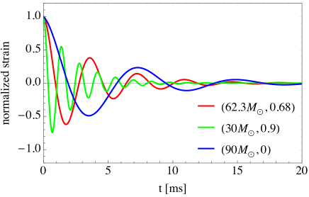
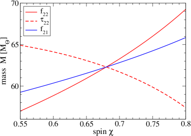
Figure 1: (Left) Normalized GW strain of the BH ringdown in GR with $(\ell,m)=(2,2)$ of the form $h_{22}(t)=e^{-t/\tau_{22}}\cos(2\pi f_{22}t)$ for various BH mass and dimensionless spin combinations. The ringdown frequency $f_{22}$ and damping time $\tau_{22}$ are taken from the fit in Berti et al. (2006). (Right) Determination of the BH mass and spin from the ringdown frequency and damping time. We used the values of $f_{\ell m}$ and $\tau_{\ell m}$ to be the GR ones with $(M,\chi)=(62.3M_{\odot},0.68)$ corresponding to GW150914 Abbott et al. (2016). GR is consistent if there is an overlap between different curves.

II General Relativity

We start by reviewing the black hole perturbation equations and eikonal QNM calculations in GR.

II.1 Perturbation Equations

We begin by considering a scalar perturbation under the Schwarzschild background following Chapter 12 of Maggiore (2018). We will then promote the perturbation equation to the tensor perturbation case.

Let us first derive the perturbation equation for the scalar field in real space. The background metric $g^{{\mbox{\tiny(B)}}}_{\mu\nu}$ is given by

$$ds^{2}=g^{{\mbox{\tiny(B)}}}_{\mu\nu}dx^{\mu}dx^{\nu}=-A_{{\mbox{\tiny GR}}}(r)dt^{2}+\frac{1}{A_{{\mbox{\tiny GR}}}(r)}dr^{2}+r^{2}(d\theta^{2}+r^{2}\sin^{2}\theta d\phi^{2})\,,$$ (1)

where $A_{{\mbox{\tiny GR}}}=1-R_{s}/r$ with $R_{s}=2M$ being the Schwarzschild radius for a BH with mass $M$. A test scalar field under this background metric follows the Klein-Gordon equation given by

$$\Box\phi=\frac{1}{\sqrt{-g^{{\mbox{\tiny(B)}}}}}\partial_{\mu}\left(\sqrt{-g^{{\mbox{\tiny(B)}}}}g_{{\mbox{\tiny(B)}}}^{\mu\nu}\partial_{\nu}\right)\phi=0\,,$$ (2)

with $g^{\mbox{\tiny(B)}}$ representing the metric determinant. Since the background metric is spherically symmetric, one can expand the scalar field $\phi$ in terms of the spherical harmonics $Y_{\ell m}$ as

$$\phi(t,r,\theta,\phi)=\frac{1}{r}\sum_{\ell=0}^{\infty}\sum_{m=-\ell}^{\ell}\phi_{\ell m}(t,r)Y_{\ell m}(\theta,\phi)\,.$$ (3)

Substituting Eq. (3) into Eq. (2), one finds

$$A_{{\mbox{\tiny GR}}}\partial_{r}(A_{{\mbox{\tiny GR}}}\partial_{r}\phi_{\ell m})-\partial_{t}^{2}\phi_{\ell m}-V_{\ell}^{\phi}(r)\phi_{\ell m}=0\,,$$ (4)

with

$$V_{\ell}^{\phi}(r)=A_{{\mbox{\tiny GR}}}(r)\left[\frac{\ell(\ell+1)}{r^{2}}+\frac{R_{2}}{r^{3}}\right]\,.$$ (5)

We present $V_{2}^{\phi}(r)$ in Fig. 2. Let us next move to a tortoise coordinate given by

$$x\equiv r+R_{s}\ln\frac{r-R_{s}}{R_{s}}\,.$$ (6)

$x\to\infty$ corresponds to infinity while $x\to-\infty$ corresponds to the horizon. Using $\partial_{x}r=A_{{\mbox{\tiny GR}}}$ and $A_{{\mbox{\tiny GR}}}\partial_{r}=\partial_{x}$, Eq. (4) becomes

$$\left[\partial_{x}^{2}-\partial_{t}^{2}-V_{\ell}^{\phi}(r)\right]\phi_{\ell m}(t,r)=0\,.$$ (7)

Let us next look at Fourier modes. Substituting

$$\phi_{\ell m}(t,r)=\int^{\infty}_{-\infty}\frac{d\omega}{\sqrt{2\pi}}\tilde{\phi}_{\ell m}(\omega,r)e^{-i\omega t}\,,$$ (8)

to Eq. (7), we find

$$\left[-\partial_{x}^{2}+V_{\ell}^{\phi}(r)\right]\tilde{\phi}_{\ell m}=\omega^{2}\tilde{\phi}_{\ell m}\,.$$ (9)

Figure 2: Various potentials in GR with $\ell=2$ as a function of $r$ in the unit $M=1$. We show $V_{2}^{\phi}$ (red), $V_{2}^{-}$ (green) and $V_{2}^{+}$ (blue).

So far, we have focused on a scalar perturbation (with spin $s=0$) under a Schwarzschild background, but the structure of the tensor perturbation equation is the same as in Eq. (9):

$$\partial_{x}^{2}\psi_{\pm}+[\omega^{2}-V_{\ell}^{\pm}]\psi_{\pm}=0\,,$$ (10)

where the indices $+$ and $-$ refer to the polar (or even-parity) and axial (odd-parity) modes respectively and we drop the indices $\ell m$ for simplicity. Notice that these two perturbation modes decouple. For axial modes, $\psi_{-}$ is the Regge-Wheeler function (a linear combination of axial metric perturbation components) and the Regge-Wheeler potential $V_{\ell}^{-}$ is given by

$$V_{\ell}^{-}(r)\equiv A_{{\mbox{\tiny GR}}}(r)\left[\frac{\ell(\ell+1)}{r^{2}}-3\frac{R_{s}}{r^{3}}\right]\,.$$ (11)

On the other hand, for polar modes, $\psi_{+}$ is the Zerilli function (a linear combination of polar metric perturbation components) and the Zerilli potential $V_{\ell}^{+}$ is given by

$$V_{\ell}^{+}(r)\equiv A_{{\mbox{\tiny GR}}}(r)\frac{2\left[\Lambda^{2}(\Lambda+1)r^{3}+3\Lambda^{2}r^{2}+9\Lambda r+9\right]}{r^{3}(\Lambda r+3)^{2}}\,,$$ (12)

with $\Lambda=(\ell-1)(\ell+2)/2$. $V_{2}^{\pm}(r)$ are shown in Fig. 2. Observe that these potentials for metric perturbations are smaller than that for the scalar perturbation. Notice also that the peak locations are all at around $r=3M$ which is the location of the photon ring.

We can understand the condition for deriving QNM frequencies by considering a scattering problem of waves under the above potential. The asymptotic behaviors of $\psi_{\pm}$ is given by

$$\psi_{\pm}\sim\begin{cases}\mathcal{A}_{i}(\omega)e^{+i\omega x}+\mathcal{A}_{r}(\omega)e^{-i\omega x}&(x\to-\infty)\,,\\ \mathcal{A}_{t}(\omega)e^{+i\omega x}&(x\to+\infty)\,,\end{cases}$$ (13)

where $\mathcal{A}_{i}$, $\mathcal{A}_{r}$ and $\mathcal{A}_{t}$ are the amplitude for the initial, reflected and transmitted waves respectively. The condition to compute QNM is

$$\mathcal{A}_{i}(\omega)=0\,.$$ (14)

Namely, we impose the wave to be purely ingoing at the horizon while purely outgoing at infinity. Although the potentials for the axial and polar modes are different, QNM frequencies for these modes are identical. This intriguing property is called isospectrality.

II.2 Eikonal QNM Calculations

We now review analytic estimates for QNM frequencies in GR within the eikonal (high frequency) approximation. We refer the readers to e.g. Glampedakis and Silva (2019) for more details. Given the isospectrality, we focus on the axial modes.

Eikonal approximation begins by making the following ansatz

$$\psi_{\pm}=\mathcal{A}_{\pm}(x)e^{iS_{\pm}(x)/\epsilon}\,,$$ (15)

for amplitude function $\mathcal{A}_{\pm}$ and phase function $S_{\pm}$ with $\epsilon\sim\ell^{-1}\ll 1$. Substituting Eq. (15) to Eq. (10), we find

$$\partial_{x}^{2}\mathcal{A}_{\pm}+\frac{i}{\epsilon}[2(\partial_{x}S_{\pm})(\partial_{x}\mathcal{A}_{\pm})+\mathcal{A}_{\pm}\partial_{x}^{2}S_{\pm}]+\left\{\omega^{2}-\frac{1}{\epsilon^{2}}(\partial_{x}^{2}S_{\pm})^{2}-A_{\mbox{\tiny GR}}\left[\frac{\ell(\ell+1)}{r^{2}}-3\frac{R_{s}}{r^{3}}\right]\right\}\mathcal{A}_{\pm}=0\,.$$ (16)

In the double expansion of $\epsilon\ll 1$ and $\ell\gg 1$, the above equation reduces to

$$-\frac{1}{\epsilon^{2}}(\partial_{x}S_{\pm})^{2}+\omega^{2}-\ell^{2}U=0\,,$$ (17)

to leading order with $U(r)\equiv A_{\mbox{\tiny GR}}(r)/r^{2}$. Notice that $\omega=\mathcal{O}(\ell)$ since $\ell\sim 1/\epsilon$.

For QNMs, we want $S_{\pm}(x)\to+\omega x$ for $x\to+\infty$ and $S_{\pm}(x)\to-\omega x$ for $x\to-\infty$, and $S_{\pm}$ to take its minimum value at the peak location $r=r_{m}=3M$ at the leading eikonal order for the potential $U$. To check this, we can take the derivative of Eq. (17) with respect to $x$ to yield

$$\frac{2}{\epsilon^{2}}(\partial_{x}S_{\pm})(\partial_{x}^{2}S_{\pm})=-\ell^{2}\frac{dr}{dx}\frac{dU}{dr}\,.$$ (18)

Thus, at the potential peak, $(dU/dr)_{m}=0$ and $(\partial_{x}S_{\pm})_{m}=0$ where the subscript $m$ indicates that the quantity is evaluated at $r=r_{m}$.

Let us now derive the real QNM frequency to leading eikonal order. We evaluate Eq. (17) at $r=r_{m}$ and impose $(\partial_{x}S_{\pm})_{m}=0$ to yield

$$\omega_{R}^{(0)}=\ell\sqrt{U_{m}}=\frac{\ell}{3\sqrt{3}M}\,,$$ (19)

where the superscript (0) indicates that this frequency is the leading eikonal contribution.

As mentioned in Sec. I, there is a correspondence between QNM frequencies and null geodesic properties in GR. For example, the real part of the QNM frequency is approximately related to the orbital angular frequency $\Omega_{\mathrm{ph}}$ at the photon ring $r_{\mathrm{ph}}$ as

$$\omega_{R}=\ell\,\Omega_{\mathrm{ph}}\,,$$ (20)

where

$$\Omega_{\mathrm{ph}}=\frac{\sqrt{A_{\mbox{\tiny GR}}(r_{\mathrm{ph}})}}{r_{\mathrm{ph}}}\,.$$ (21)

The photon ring location is obtained by solving

$$2A_{\mbox{\tiny GR}}(r_{\mathrm{ph}})=r_{\mathrm{ph}}A_{\mbox{\tiny GR}}^{\prime}(r_{\mathrm{ph}})\,,$$ (22)

to yield $r_{\mathrm{ph}}=3M$ (which coincides with the potential peak location $r_{m}$ in the eikonal limit). Plugging this into Eq. (21), we find $\Omega_{\mathrm{ph}}=1/(3\sqrt{3}M)$ and Eq. (20) agrees with Eq. (19).

To find the imaginary QNM frequency, we need to go to the next-to-leading eikonal order. For $\omega=\omega_{R}+i\omega_{I}$ with $\omega_{R},\omega_{I}\in\mathbb{R}$, we make the following ansatz:

$$\omega_{R}=\omega_{R}^{(0)}+\omega_{R}^{(1)}+\mathcal{O}(\ell^{-1})\,,\quad\omega_{I}=\omega_{I}^{(1)}+\mathcal{O}(\ell^{-1})\,,$$ (23)

where the superscript $(N)$ indicates the quantity to be at $N$th order in the eikonal expansion or $\mathcal{O}(\ell^{1-N})$. Substituting this to Eq. (16), expand in $\epsilon\ll 1$ and $\ell\gg 1$ and keeping only the contribution at $\mathcal{O}(\ell,\epsilon^{-1})$, we find

$$\frac{2i}{\epsilon}(\partial_{x}S_{\pm})(\partial_{x}\mathcal{A}_{\pm})+\left(\frac{i}{\epsilon}\partial_{x}^{2}S_{\pm}+2i\omega_{R}^{(0)}\omega_{I}^{(1)}+2\omega_{R}^{(0)}\omega_{R}^{(1)}-\ell U\right)\mathcal{A}_{\pm}=0\,.$$ (24)

To proceed further, we need $(\partial_{x}^{2}S_{\pm})_{m}$. To find this, we Taylor expand Eq. (17) about $r=r_{m}$ to yield

$$\frac{1}{\epsilon^{2}}(\partial_{x}S_{\pm})^{2}=-\frac{\ell^{2}}{2}U_{m}^{\prime\prime}(r-r_{m})^{2}\,.$$ (25)

Taking the positive root for $\partial_{x}S_{\pm}$ and differentiate with respect to $x$, we find

$$\frac{1}{\epsilon}(\partial_{x}^{2}S_{\pm})=\frac{\ell}{\sqrt{2}}\frac{dr}{dx}\sqrt{|U_{m}^{\prime\prime}|}\,.$$ (26)

We are now ready to evaluate the imaginary QNM frequency and the sub-leading QNM real frequency. Regarding the former, we take the imaginary part of Eq. (24), together with Eqs. (19) and (26), and evaluate it at $r_{0}$ to find

$$\omega_{I}^{(1)}=-\frac{1}{2\epsilon}\frac{(\partial_{x}^{2}S_{\pm})_{m}}{\omega_{R}^{(0)}}=-\frac{1}{2}\left(\frac{dr}{dx}\right)_{m}\sqrt{\frac{|U_{m}^{\prime\prime}|}{2U_{m}}}=-\frac{1}{6\sqrt{3}M}\,.$$ (27)

Regarding the latter, we take the real part of Eq. (24) to find

$$\omega_{R}^{(1)}=\frac{\ell U_{m}}{2\omega_{R}^{(0)}}=\frac{1}{2}\sqrt{U_{m}}=\frac{1}{6\sqrt{3}M}\,.$$ (28)

Together with $\omega_{R}^{(0)}$, we find

$$\omega_{R}=\left(\ell+\frac{1}{2}\right)\sqrt{U_{m}}=\frac{1}{3\sqrt{3}M}\left(\ell+\frac{1}{2}\right)\,.$$ (29)

Figure 3 compares the above eikonal results with the numerical values at various $\ell$. The leading eikonal results at $\mathcal{O}(\ell)$ agrees with the numerical ones within an error of $4.5\%$. Interestingly, the agreement becomes worse if we include the next-to-leading contribution at $\mathcal{O}(\ell^{0})$. This problem is cured by including the next-to-next-to-leading contribution at $\mathcal{O}(\ell^{-1})$ found in Iyer (1987) via a WKB approximation. Now the two results agree within an error of $3.4\%$.

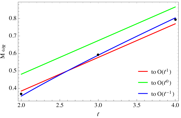
Figure 3: Comparison of the analytic estimate for the real QNM frequency at various $\ell$ in GR with the numerical values Berti et al. (2006) (black dots). For the former, we present the result with the leading eikonal contribution (red), and including the next-to-leading contribution (green) in Eq. (29). We also present the result including the next-to-next-to-leading contribution taken from Iyer (1987) through the WKB approximation.

III Scalar Gauss-Bonnet Gravity

We now review the application of the eikonal technique to theories beyond GR. We mainly review the work in Bryant et al. (2021) which applies the eikonal analysis to another higher curvature theory called sGB gravity.

III.1 Theory and Black Hole Solution

The action for this theory in vacuum is given by Nojiri et al. (2005); Yagi (2012); Antoniou et al. (2018a, b)

$$S=\frac{1}{16\pi}\int d^{4}x\sqrt{-g}\left[R-\frac{1}{2}\partial_{\mu}\phi\partial^{\mu}\phi+\alpha f(\phi)\mathcal{G}\right]\,,$$ (30)

where $\phi$ is the scalar (dilaton) field, $R$ is the Ricci scalar, $\alpha$ is the coupling constant, $f$ is an arbitrary function of $\phi$ and $\mathcal{G}$ is given by

$$\mathcal{G}=R_{\alpha\beta\mu\nu}R^{\alpha\beta\mu\nu}-4R_{\alpha\beta}R^{\alpha\beta}+R^{2}\,,$$ (31)

with $R_{\alpha\beta\mu\nu}$ and $R_{\alpha\beta}$ being the Riemann and Ricci tensors respectively. $f(\phi)\propto\exp(\gamma\phi)$ for a constant $\gamma$ corresponds to EdGB gravity while $f(\phi)\propto\phi$ corresponds to shift-symmetric sGB gravity. SGB gravity and its extension is motivated also by cosmology, such as inflation Oikonomou and Fronimos (2021); Oikonomou (2021). The coupling constant $\alpha$ has been constrained by various observations, including low-mass x-ray binaries Yagi (2012), gravitational waves from binary black holes Nair et al. (2019); Yamada et al. (2019); Tahura et al. (2019); Perkins et al. (2021); Wang et al. (2021); Lyu et al. (2022); Perkins and Yunes (2022) and neutron star observations Pani et al. (2011a); Saffer and Yagi (2021) (see also a recent work in Herrero-Valea (2021)).

The field equations are given by

$$\Box\phi =\alpha f^{\prime}(\phi)\mathcal{G}\,,$$ (32)

$$G_{\alpha\beta} =\frac{1}{2}\partial_{\alpha}\phi\,\partial_{\beta}\phi-\frac{1}{4}g_{\alpha\beta}\partial_{\mu}\phi\,\partial^{\mu}\phi-\alpha\mathcal{K}_{\alpha\beta}\,,$$ (33)

where $G_{\alpha\beta}$ is the Einstein tensor while $\mathcal{K}_{\alpha\beta}$ is given by

$$\mathcal{K}_{\alpha\beta}=(g_{\alpha\mu}g_{\beta\nu}+g_{\alpha\nu}g_{\beta\mu})\,\epsilon^{\rho\nu\sigma\kappa}\nabla_{\lambda}\,[{}^{\ast}{R}^{\mu\lambda}{}_{\sigma\kappa}\partial_{\rho}f(\phi)]\,,$$ (34)

with the dual Riemann tensor ${}^{*}R^{\alpha\beta}{}_{\gamma\delta}=\epsilon^{\alpha\beta\mu\nu}R_{\mu\nu\gamma\delta}$ and $\epsilon^{\alpha\beta\mu\nu}$ representing the Levi-Civita tensor.

In this theory, a non-rotating black hole solution is known analytically within the small coupling approximation ($\alpha\ll M^{2}$). To $\mathcal{O}(\alpha^{2})$, the metric is given by Kanti et al. (1996); Yunes and Stein (2011); Pani et al. (2011b); Ayzenberg and Yunes (2014); Maselli et al. (2015)

$$ds^{2}=\bar{g}^{\mbox{\tiny(B)}}_{\mu\nu}dx^{\mu}dx^{\nu}=-A(r)dt^{2}+\frac{1}{B(r)}dr^{2}+r^{2}(d\theta^{2}+r^{2}\sin^{2}\theta d\phi^{2})\,,$$ (35)

with

$$A =1-\frac{2M}{r}-\frac{\alpha^{2}f_{0}^{\prime 2}}{rM^{3}}\left(\frac{49}{40}-\frac{M^{2}}{3r^{2}}-\frac{26M^{3}}{3r^{3}}-\frac{22M^{4}}{5r^{4}}-\frac{32M^{5}}{5r^{5}}+\frac{80M^{6}}{3r^{6}}\right)\,,$$ (36)

$$B =1-\frac{2M}{r}-\frac{\alpha^{2}f_{0}^{\prime 2}}{rM^{3}}\left(\frac{49}{40}-\frac{M}{r}-\frac{M^{2}}{r^{2}}-\frac{52M^{3}}{3r^{3}}-\frac{2M^{4}}{r^{4}}-\frac{16M^{5}}{5r^{5}}+\frac{368M^{6}}{3r^{6}}\right)\,,$$ (37)

and $f^{\prime}_{0}\equiv f^{\prime}(0)$. The background scalar field is given by

$$\phi_{0}=\frac{2\alpha f^{\prime}_{0}}{rM}\left(1+\frac{M}{r}+\frac{4M^{2}}{3r^{2}}\right)+\frac{\alpha^{2}f^{\prime}_{0}f^{\prime\prime}_{0}}{rM^{3}}\left(\frac{73}{30}+\frac{73M}{30r}+\frac{146M^{2}}{45r^{2}}+\frac{73M^{3}}{15r^{3}}+\frac{224M^{4}}{75r^{4}}+\frac{16M^{5}}{9r^{5}}\right)\,,$$ (38)

with $f^{\prime\prime}_{0}\equiv f^{\prime\prime}(0)$. The ADM mass $M_{*}$ is given in terms of the GR one $M$ as follows:

$$M_{*}=M\left(1+\frac{49}{80}\frac{\alpha^{2}f_{0}^{\prime 2}}{M^{4}}\right)\,.$$ (39)

III.2 Perturbation Equations

Next, we look at black hole perturbation equations in sGB gravity. We perturb both the metric and scalar field as

$$g_{\mu\nu}=\bar{g}^{\mbox{\tiny(B)}}_{\mu\nu}+h_{\mu\nu}\,,\quad\phi=\phi_{0}+\delta\phi\,,$$ (40)

where $h_{\mu\nu}$ and $\delta\phi$ are the metric and scalar perturbations respectively. As we will see below, $\delta\phi$ is coupled only to the polar sector of the metric perturbation, while the axial part is decoupled.

Let us begin with the axial perturbations. The master perturbation equation is given by Blázquez-Salcedo et al. (2016); Bryant et al. (2021)

$$\partial_{\bar{x}}^{2}\bar{\psi}_{-}+(C_{-}\omega^{2}-\bar{V}_{\ell}^{-})\bar{\psi}_{-}=0\,.$$ (41)

Here $\bar{x}$ is the tortoise coordinate in sGB gravity that satisfies $\partial_{r}\bar{x}=1/\sqrt{AB}$. $\bar{\psi}_{-}$ is the master variable for axial perturbation in sGB gravity, while $\bar{V}_{\ell}^{-}$ is the corresponding potential whose lengthy expression can be found in Bryant et al. (2021). The coefficient $C_{-}$ is given by

$$C_{-}=\frac{A}{A-2\alpha BA^{\prime}\phi_{0}^{\prime}f_{0}^{\prime}}\{1-2\alpha B^{\prime}\phi_{0}^{\prime}f_{0}^{\prime}+4\alpha B[{\phi_{0}^{\prime}}^{2}f_{0}^{\prime\prime}+\phi_{0}^{\prime\prime}f_{0}^{\prime}]\}\,.$$ (42)

In the limit $\alpha\to 0$, $C_{-}\to 1$ while $\bar{V}_{\ell}^{-}\to V_{\ell}^{-}$ and Eq. (41) reduces to the GR one in Eq. (10). We can further perform a coordinate transformation from $\bar{x}$ to $\tilde{x}$ to remove $C_{-}$:

$$\frac{d\tilde{x}}{d\bar{x}}=\sqrt{C_{-}}\,.$$ (43)

Equation (41) then becomes

$$\partial_{\tilde{x}}^{2}\bar{\psi}_{-}+p_{-}\partial_{\tilde{x}}\bar{\psi}_{-}+(\omega^{2}-\tilde{V}_{\ell}^{-})\bar{\psi}_{-}=0\,,$$ (44)

where $p_{-}\equiv\partial_{\bar{x}}C_{-}/(2C_{-})^{3/2}$ and $\tilde{V}_{\ell}^{-}\equiv\bar{V}_{\ell}^{-}/C_{-}$.

Next, we look at polar perturbations. The master equations for the metric and scalar perturbations under the small coupling approximation are given by Bryant et al. (2021)

$$\partial_{\bar{x}}^{2}\bar{\psi}_{+}+p_{+}\partial_{\bar{x}}\bar{\psi}_{+}+(C_{+}\omega^{2}-\bar{V}_{\ell}^{+})\bar{\psi}_{+}=a_{0}\bar{\phi}+a_{1}\partial_{\bar{x}}\bar{\phi}\,,$$ (45)

$$\partial_{\bar{x}}^{2}\bar{\phi}+(\omega^{2}-\bar{V}_{\ell}^{\phi})\bar{\phi}=b_{0}\bar{\psi}_{+}+b_{1}\partial_{\bar{x}}\bar{\psi}_{+}\,.$$ (46)

Here $\bar{\psi}_{+}$ and $\bar{\phi}$ are the master metric and scalar perturbation variables respectively. For example, $\bar{\phi}$ is given by

$$\delta\phi(t,r)=\frac{1}{\sqrt{2\pi}}\int dt\,\frac{\bar{\phi}(\omega,r)}{r}Y_{\ell m}\,e^{-i\omega t}\,.$$ (47)

The scalar potential is given by Bryant et al. (2021)

$$\bar{V}_{\ell}^{\phi}=V_{\ell}^{\phi}-\alpha f_{0}^{\prime\prime}\frac{48M^{2}(r-2M)}{r^{7}}\,,$$ (48)

while the polar metric potential $\bar{V}_{\ell}^{+}$ and other coefficients in Eqs. (45) and (46) are given in Bryant et al. (2021). Notice that the two perturbation equations are coupled. Figure 4 presents $\bar{V}_{2}^{\phi}$ and $\bar{V}_{2}^{+}$ for various $\alpha$. Notice that the potential decreases while the peak location increases as one increases $\alpha$.

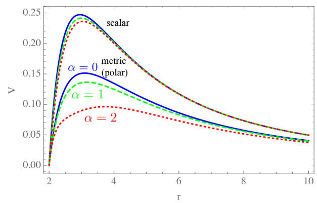
Figure 4: Scalar potential $\bar{V}_{2}^{\phi}$ (top) and metric polar potential $\bar{V}_{2}^{+}$ (bottom) as a function of $r$ for three different choices of $\alpha$ (in the unit $M=1$).

III.3 Eikonal QNM Calculations

Let us now apply the eikonal technique to find QNM frequencies in sGB gravity  Bryant et al. (2021). We will look at axial and polar sectors separately.

III.3.1 Axial Perturbations

We begin by studying the axial perturbations. The procedure is the same as that in GR described in Sec. II.2. We start by making an ansatz

$$\bar{\psi}_{-}=\bar{\mathcal{A}}_{-}(\tilde{x})e^{i\bar{S}_{-}(\tilde{x})/\epsilon}\,,$$ (49)

with the amplitude function $\bar{\mathcal{A}}_{-}$ and the phase function $\bar{S}_{-}$. Substituting this to Eq. (44), expand in $\epsilon\ll 1$ and $\ell\gg 1$ and dropping $\partial_{\tilde{x}}\bar{S}_{-}$, we find

$$\omega^{(0)}_{R}=\ell\sqrt{\bar{U}_{m}}=\ell\,\left[\frac{A-2\alpha BA^{\prime}\phi_{0}^{\prime}f^{\prime}_{0}}{r\left(r-4\alpha B\phi_{0}^{\prime}f^{\prime}_{0}\right)}\right]^{1/2}_{m}\,,$$ (50)

where $\bar{U}$ is given by

$$\bar{V}_{\ell}^{-}=\ell^{2}\bar{U}+\mathcal{O}(\ell)\,.$$ (51)

We also need to account for the sGB correction to the peak location of the potential. Solving $\bar{U}^{\prime}=0$, we find

$$r_{m}=3M+\frac{6577}{19440}\frac{\alpha^{2}f_{0}^{\prime 2}}{M^{3}}\,,$$ (52)

to $\mathcal{O}(\alpha^{2})$. Thus, under the small coupling approximation, we find

$$\omega_{R}^{(0)}=\frac{\ell}{3\sqrt{3}M}\left(1-\frac{71987}{174960}\frac{\alpha^{2}f_{0}^{\prime 2}}{M^{4}}\right)\,.$$ (53)

We comment on the correspondence between QNM and null geodesics. Notice that Eq. (50) is different from

$$\omega_{R}=\ell\frac{\sqrt{A(r_{\mathrm{ph}})}}{r_{\mathrm{ph}}}$$ (54)

obtained by combining Eqs. (20) and (21). In particular, Eq. (50) depends on the background scalar field. Thus, the correspondence does not work in non-GR theories in general. However, for sGB gravity up to $\mathcal{O}(\alpha^{2})$, the contribution from the background scalar field cancels with the correction to $r_{\mathrm{ph}}$ and one does recover Eq. (53) by using Eq. (54) with $r_{\mathrm{ph}}=3M$. Thus, the null geodesic correspondence still holds, at least up to $\mathcal{O}(\alpha^{2})$ in the axial sector.

We now move to finding the sub-leading contribution to the axial QNM frequencies. We make the same ansatz to $\omega$ as in Eq. (23). The only difference from the GR case is to replace $U$ by $\bar{U}$ and $x$ to $\tilde{x}$. For the real frequency, we find $\omega_{R}^{(1)}=\sqrt{\bar{U}_{m}}/2$ and

$$\omega_{R}=\left(\ell+\frac{1}{2}\right)\sqrt{\bar{U}_{m}}= \left(\ell+\frac{1}{2}\right)\left[\,\frac{A-2\alpha BA^{\prime}\phi_{0}^{\prime}f^{\prime}_{0}}{r\left(r-4\alpha B\phi_{0}^{\prime}f^{\prime}_{0}\,\right)}\,\right]^{1/2}_{m}$$

$$= \frac{1}{3\sqrt{3}M}\left(\ell+\frac{1}{2}\right)\left(1-\frac{71987}{174960}\frac{\alpha^{2}f_{0}^{\prime 2}}{M^{4}}\right)\,.$$ (55)

For the imaginary frequency, we find

$$\omega_{I}^{(1)}=-\frac{1}{2}\left(\frac{dr}{d\tilde{x}}\right)_{m}\sqrt{\frac{|\bar{U}_{m}^{\prime\prime}|}{2\bar{U}_{m}}}=-\frac{1}{6\sqrt{3}M}\left(1-\frac{121907}{174960}\frac{\alpha^{2}f_{0}^{\prime 2}}{M^{4}}\right)\,,$$ (56)

under the small coupling approximation.

III.3.2 Polar Perturbations

We next turn our attention to the polar sector. This time, the situation is quite different from the GR case as the perturbation equations for the metric and scalar fields are coupled. Our starting point is the same by making the following ansatz:

$$\bar{\psi}_{+}=\bar{\mathcal{A}}_{+}(\tilde{x})e^{i\bar{S}_{+}(\tilde{x})/\epsilon}\,,\quad\bar{\phi}=\bar{\mathcal{A}}_{\phi}(\tilde{x})e^{i\bar{S}_{+}(\tilde{x})/\epsilon}\,.$$ (57)

Notice that the phase functions are common in the two perturbations. Using this, we find that the equation for $\omega$ is biquadratic instead of quadratic:

$$\omega^{4}+F(\epsilon,\alpha,\ell,r_{m},\bar{S}_{+,m},\bar{\mathcal{A}}_{+,m},\bar{\mathcal{A}}_{\phi,m})\,\omega^{2}+G(\epsilon,\alpha,\ell,r_{m},\bar{S}_{+,m},\bar{\mathcal{A}}_{+,m},\bar{\mathcal{A}}_{\phi,m})=0\,.$$ (58)

Working in the small coupling assumption of $\alpha\ll\epsilon$ (and setting the book-keeping parameter $\epsilon$ to 1), we find the solution to $\omega^{2}$ as

$$\omega_{\pm}^{2}=\frac{\ell^{2}}{27M^{2}}\left\{\,1+\frac{1}{\ell}\left(1-27i\frac{S^{\prime\prime}_{+,m}}{\ell}\right)\pm\frac{8\,\alpha^{2}f_{0}^{\prime 2}{}}{27M^{4}}\left[\,\ell^{2}+2\left(\ell-4iS_{+,m}^{\prime\prime}\right)\,\right]\,\right\}\,,$$ (59)

with

$$S_{+,m}^{\prime\prime}=\frac{\ell}{27M^{2}}\left(1-\frac{560}{2187}\frac{\alpha^{2}\ell f_{0}^{\prime 2}}{M^{4}}\right)\,.$$ (60)

Notice that there are two solutions for $\omega^{2}$. The mode with the $+(-)$ sign corresponds to the scalar-led (gravity-led) mode Blázquez-Salcedo et al. (2016). From the above equations, the leading eikonal contribution to the real and imaginary frequencies are given by

$$\omega_{R\pm}= \frac{\ell}{3\sqrt{3}M}\left(\,1\pm\frac{4}{27}\frac{\alpha^{2}\ell^{4}f_{0}^{\prime 2}{}}{M^{4}}\,\right)\,,$$ (61)

$$\omega_{I\pm}= -\frac{1}{6\sqrt{3}M}\left(1\pm\frac{44}{729}\frac{\alpha^{2}\ell^{2}f_{0}^{\prime 2}}{M^{4}}\right)\,.$$ (62)

Comparing these with the axial results (Eqs. (III.3.1) and (56)), it is clear that the isospectrality is broken in sGB gravity. Moreover, there are three independent QNM frequencies: axial (gravity-led) mode, polar gravity-led mode, and polar scalar-led mode.

III.4 Summary of Eikonal Expressions

We end this section by summarizing the eikonal expressions and comparing them with the numerical results in Blázquez-Salcedo et al. (2016). We convert the expressions in terms of the ADM mass $M_{*}$ using Eq. (39).

III.4.1 Axial Perturbations

The axial QNM frequencies are given as follows:

$$\omega_{R} =\left(\ell+\frac{1}{2}\right)\frac{1}{3\sqrt{3}M_{*}}\left(1+\frac{4397}{21870}\frac{\alpha^{2}f_{0}^{\prime 2}}{M_{*}^{4}}\right),$$ (63)

$$\omega_{I} =-\frac{1}{6\sqrt{3}M_{*}}\left(1-\frac{1843}{21870}\frac{\alpha^{2}f_{0}^{\prime 2}}{M_{*}^{4}}\right).$$ (64)

III.4.2 Polar Perturbations

For polar perturbations, the real frequency of the gravity-led mode is given by

$$\omega_{R-}=\frac{\ell}{3\sqrt{3}M_{*}}\left(\,1-\frac{4}{27}\frac{\alpha^{2}\ell^{4}f_{0}^{\prime 2}{}}{M_{*}^{4}}\,\right)\,.$$ (65)

For the scalar-led mode, it turns out that the leading eikonal results are not sufficient to accurately describe the numerical results. For this reason, we include the higher order contributions:

$$\omega_{R+}=\frac{\sqrt{\ell(\ell+1)}}{3\sqrt{3}M_{*}}\left[1-\frac{8\alpha}{27\ell(\ell+1)M_{*}^{2}}f^{\prime\prime}_{0}+\frac{4}{27}\frac{\alpha^{2}f_{0}^{\prime 2}}{(\ell+1)M_{*}^{4}}\left(\ell^{3}+2\ell^{2}+\frac{5249\ell}{960}+\frac{1323}{320}\right)\right]\,.$$ (66)

The imaginary frequencies for the gravity-led and scalar-led modes are given by

$$\omega_{I\pm}=-\frac{1}{6\sqrt{3}M_{*}}\left(1\pm\frac{44}{729}\frac{\alpha^{2}\ell^{2}f^{\prime\prime}_{0}}{M_{*}^{4}}\right)\,.$$ (67)

III.4.3 Comparison with Numerical Results

Let us now compare the above eikonal results with the numerical ones. We focus on EdGB gravity with $f=\exp(\phi)/4$ and thus $f^{\prime}_{0}=1/4$. Figure 5 compares the real QNM frequencies of the eikonal results found here with the numerical ones in Blázquez-Salcedo et al. (2016) for the three modes as a function of $\alpha$. Notice that the eikonal expressions can accurately describe the numerical results when $\alpha$ is small, where the small coupling approximation is valid. On the other hand, the agreement between eikonal and numerical results for the imaginary QNM frequency is not as good as the real frequency case and requires further study Bryant et al. (2021).

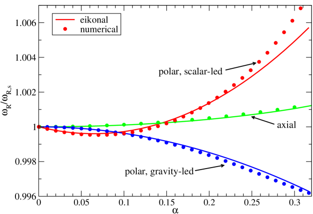
Figure 5: Various $\ell=2$ real QNM frequencies in EdGB gravity with $f_{0}^{\prime}=1/4$ Bryant et al. (2021). We present the frequency normalized by the GR Schwarzschild value $(\omega_{R,S})$ as a function of the coupling constant $\alpha$ (in the unit $M=1$) for the analytic eikonal (solid curves) and numerical Blázquez-Salcedo et al. (2016) (dots) results. We show the frequencies for axial perturbation (green), polar gravity-led perturbation (blue) and polar scalar-led perturbation (red). The eikonal results are obtained within the small coupling approximation and thus is valid only when $\alpha$ is small.

IV Discussions

The eikonal method reviewed here can be applied to theories other than GR and sGB gravity. For example, Glampedakis and Silva Glampedakis and Silva (2019) have applied it to dynamical Chern-Simons gravity Alexander and Yunes (2009) which is a parity-violating gravity. In the action, a parity-violating term that is quadratic in curvature (Pontryagin density) is coupled to a pseudoscalar field. QNM frequencies of BHs in this theory have been computed in Yunes and Sopuerta (2008); Molina et al. (2010); Wagle et al. (2021); Srivastava et al. (2021). For non-rotating BHs, the background solution is the same as GR (Schwarzschild) and polar perturbation equations are identical to GR. On the other hand, the axial perturbation is coupled to the scalar perturbation, though the axial perturbation potential is identical to the GR Regge-Wheeler potential. Hence, the analysis is much simpler than the sGB case.

In this chapter, we have focused on non-rotating BHs. A natural extension is to consider rotating BHs. In many theories, analytic BH solutions with arbitrary rotation have not been found yet while slowly-rotating solutions are available. This is indeed the case with sGB gravity Pani et al. (2011b); Ayzenberg and Yunes (2014); Maselli et al. (2015) and dynamical Chern-Simons gravity Yunes and Pretorius (2009); Pani et al. (2011b); Ali-Haimoud and Chen (2011); Yagi et al. (2012); Maselli et al. (2017). A first attempt on applying the eikonal analysis to slowly-rotating BHs to first order in spin in non-GR theories has been carried out in Silva and Glampedakis (2020).