Nonlinear Control Allocation: A Learning Based Approach

Abstract

Modern aircraft are designed with redundant control effectors to cater for fault tolerance and maneuverability requirements. This leads to an over-actuated aircraft which requires a control allocation scheme to distribute the control commands among effectors. Traditionally, optimization based control allocation schemes are used; however, for nonlinear allocation problems these methods require large computational resources. In this work, a novel ANN based nonlinear control allocation scheme is proposed. To start, a general nonlinear control allocation problem is posed in a different perspective to seek a function which maps desired moments to control effectors. Few important results on stability and performance of nonlinear allocation schemes in general and this ANN based allocation scheme, in particular, are presented. To demonstrate the efficacy of the proposed scheme, it is compared with standard quadratic programming based method for control allocation.

I Introduction

Traditionally, there are three primary control effectors in aircraft flight control: aileron, elevator, and rudder. They are usually designed utilizing one control effector for each degree of freedom. However, due to the increased requirements on the reliability, maneuverability and survivability of modern and futuristic aircraft, control effectors are no longer limited to these three conventional effectors. In newer designs, often a large number of control effectors are used to provide reconfiguration flexibility and required redundancy for the fault-tolerance [1, 2]. Redundancy in control effectors can also be utilized to enhance an airplane’s performance envelope. For example, thrust vectoring augments the dog-fighting capability of the F-22 Raptor, and permits maneuvers such as Pugachev’s Cobra in other aircraft [3].

The problem of distributing control commands to several control actuators is known as Control Allocation. Several tools and approaches have been proposed and used to manage redundancy and to distribute the desired control effort among a set of actuators [3, 4]. A conventional and most straightforward approach is to manually distribute the control actuators into three sets, and use each set of control actuators as ‘elevator’ (to produce pitching moment), ‘aileron’ (to produce rolling moment), and ‘rudder’ (to produce yawing moment). This method, formally known as Explicit Ganging, usually works well for aircraft having a relatively lesser degree of over-actuation but not so for a multi-rotor or fixed-wing aircraft with a large number of control effectors.

Another much more sophisticated strategy is to distinguish the regulation or tracking aspect of the problem from a control distribution perspective. Fig. 1 portrays how control law specifies desired control effort (desired forces/moments) and how a separate control allocator is introduced in the control loop to allocate the desired control effort among various actuators. In an over-actuated system the desired commands can be achieved with multiple combinations of control effector deflections. Using a control allocation method, the desired commands are distributed over the available control effector suite in such a way that the desired control effect is produced, along with fulfilling some additional objectives like minimization of deflections, drag or radar cross-section (RCS) etc.

[CAblkDiag]TikzDatabase.tikz

Figure 1: Feedback-loop structure with control allocation

At present, most common practice is to use control allocation methods that assume a linear relationship between effector deflections and resulting control moments. Such methods include direct allocation [5, 6, 7], daisy chaining [8], redistributed pseudo-inverse or cascaded generalized inverse [4], and methods based on linear programming [7, 9] and quadratic programming [7][10]. Generally, for most practical applications, optimization based methods are preferred due to their accuracy and flexibility [11]. This assumption of linearity allows us to use control allocation through computationally efficient algorithms. However, control allocation problem of an aircraft is inherently nonlinear and coupled, especially the cross-channel effectiveness of surfaces is highly nonlinear in nature [12, 13].

The problem of nonlinear control allocation is challenging due to the possibility of local minima and computational issues [11], and so far literature on this subject is limited. A more intuitive way is to treat the nonlinear mapping directly through the sequential quadratic programming [14], but the computational complexity could be overwhelming. Piecewise-linear [15, 16] and time-varying affine [17] approximations of nonlinear problems have also been studied. For practical purposes most modern aircraft employ affine control allocation schemes [4, 11], either in absolute or incremental form, due to their accuracy and computational efficiency as compared to other methods. However, these affine methods still require computation of the local Jacobian matrix and offset vector, and solving a linear or quadratic program at each sampling instant. This not only requires large onboard computational power, but also an accurate model of effectiveness function in onboard computer, which can take significant storage depending upon the number of effectors, flight envelope and accuracy of model.

Artificial Neural Networks (ANNs) are widely used computing systems that mimic biological neural networks that are present in an animal brain. These systems learn to do some task by considering given examples, generally without task-specific programming. There are many types of ANNs used for different type of machine learning tasks, e.g. Fully Connected ANN, Convolutional Neural Network (CNN), Recurrent Neural Networks (RNN) etc. In this paper, we will only consider Fully Connected ANNs. These ANNs have proved to be excellent function approximators and can approximate almost all nonlinear functions with arbitrary accuracy (Universal Approximation Theorems) [18]. In spite of widespread use of ANNs in almost all fields of engineering and science, their employment in control allocation has been limited.

Initially, Grogan et al. [19] explored the use of an ANN based scheme for linear control allocation problems, with a single hidden layer, and compared it with direct allocation for F/A-18 HARV aircraft. However, based on training limitations and accuracy issues they concluded that ANN based scheme is not suitable for practical applications. It must be noted that their work was done in 1994, and since then, there has been a manifold improvement in the machine learning tools. They concluded that direct allocation is computationally efficient than ANN for a linear allocation problem, but for nonlinear allocation problems these optimization-based methods are though accurate but highly computationally expensive. An important difference in our work is the use of Rectified Linear Unit (ReLU) activation function which results in better training performance as compared to the hyperbolic-tangent activation function which they used. Quite recently, there has been some research done on machine learning based control allocation schemes. Chen [20] has used RNNs for linear control allocation problems. Huan et al. [21] have used deep auto-encoders for nonlinear control allocation problem, where they considered two separate networks one (encoder) acting as an allocator while the other (decoder) mimics the system. Vries et al. [22] has used reinforcement learning approach for nonlinear control allocation.

In this research, we pose a general nonlinear control allocation problem in a different perspective, that is to seek a function which maps desired moments to control effectors. This view of control allocation, is similar to pseudo-inverse methods for linear allocation problems, but differs with optimization-based methods for either linear or nonlinear allocation problems, which try to find control effector commands for a given desired moment vector. Due to the excellent function approximation properties of ANN, we use them to approximate this map between desired moments and control effectors, and convert the allocation problem to a machine learning problem. We present training methodologies for different types of allocation problems, e.g. effector prioritization, fault tolerance, reconfiguration etc. Later on we present few important results on stability and performance of nonlinear allocation schemes in general and this ANN based allocation scheme in particular. Then to demonstrate the efficacy of the proposed scheme, we compare the results with standard methods of control allocation for a miniature tailless flying-wing research aircraft [23, 24].

II Preliminaries

II-A Nonlinear Control Allocation

The general nonlinear control allocation problem is defined as follows: find the control vector $u$ such that,

$$\mathcal{G}(u,\sigma)=\tau_{d}$$ (1)

where $u\in\mathcal{U}\subseteq\mathbb{R}^{n}$ is actual input vector of the system being controlled, $\tau_{d}\in\mathbb{R}^{m}$ is vector of desired moments (virtual control), $\sigma\in\mathcal{S}$ is some state vector, and $\mathcal{G}:\mathcal{U}\,\times\,\mathcal{S}\mapsto\mathcal{T}\subseteq\mathbb{R}^{m}$ is control effectiveness mapping, and is assumed to be at least continuous in both $u$ and $\sigma$, where $\mathcal{T}$ (mentioned below) is known as Attainable Moment Set (AMS). Following are the precise definitions we will be using in later sections:

Definition 1.

The pointwise AMS is defined as,

$$\mathcal{T}_{\sigma}\triangleq\mathcal{G}\left(\mathcal{U},\sigma\right),\quad\forall\,\sigma\in\mathcal{S}$$ (2)

and total or complete AMS, or just AMS, is defined as

$$\mathcal{T}\triangleq\bigcup_{\sigma\in\mathcal{S}}\mathcal{T}_{\sigma}$$ (3)

The system of equations Eq. (1) being underdetermined, usually possess multiple solutions, only if the constraints on input $u$ are strongly satisfied, otherwise no exact solution exists. Numerous methods have been proposed [4, 11] to solve this constrained allocation problem, especially for cases when $\mathcal{G}$ is a constant linear map from $\mathcal{U}$ to $\mathcal{T}$, for example Redistributed Pseudo-Inverse (RPI) or Cascaded Generalized Inverse (CGI), Direct-Allocation, Daisy-Chaining, and Optimization based methods.

For nonlinear $\mathcal{G}$, which is usually the case for modern over-actuated aircraft, it is a common practice to convert a nonlinear problem into a locally affine allocation problem at each sampling instant. At any sampling instant (1) can be approximately written as;

$$Gu\approx\bar{\tau}_{d}=\tau_{d}-\varepsilon$$ (4)

where

$$G=\left.\frac{\partial\mathcal{G}}{\partial u}\right|_{(u_{0},\sigma_{0})},\text{and}\;\varepsilon=\mathcal{G}(u_{0},\sigma_{0})-Gu_{0}$$

Eq. 4 can be solved using any linear allocation method, depending upon the requirements, for which highly efficient tools are available. However, due to their superior performance constrained optimization based methods are generally preferred for practical applications over pseudo-inverse based methods [11].

General nonlinear allocation problem (1) can be posed as following weighted constrained optimization problem: given $\tau_{d}\in\mathcal{T}_{\sigma}$ and $\sigma\in\mathcal{S}$ solve

$$\min_{u}\quad\big{\|}\mathcal{G}(u,\sigma)-\tau_{d}\big{\|}^{2}_{W},\qquad$$ (5)

subject to:

$$u\in\mathcal{U}$$

where, $\|\cdot\|_{W}$ represents the weighted 2-norm and is defined as, $\|x\|_{W}^{2}\triangleq x^{\top}Wx$, where $W$ is a symmetric positive definite matrix. It must be noted that in this case, for a given $\tau_{d}$, optimization gives a vector $u\in\mathcal{U}$.

II-B Artificial Neural Networks (ANNs)

Artificial Neural Networks (ANNs) are self-learning algorithms that are created in such a way as to mimic the way a human brain investigates and processes information using an interlocked mesh of neurons. ANNs are substantial layered computation paradigms consisting of simple processing elements that can solve problems which are deemed complex in nature by human or statistical standards, given that enough learning data sets are available for training. In the past few years, the adaptive nature and excellent function approximation capability of ANNs have led to their prevalent use in a variety of applications [25, 26].

Structure of an ANN consists of multiple layers of artificial neurons. Each neuron receives a vector from the previous layer as its input; and applies an affine transformation followed by a static nonlinear activation function. Therefore, the output of $i$th layer is defined as,

$$\begin{split}z_{i}&=\Theta_{i}a_{i-1}+b_{i}\\ a_{i}&=\phi(z_{i})\end{split}$$ (6)

If the network has $s_{i-1}$ neurons in $(i-1)$-th layer, and $s_{i}$ neurons in $i$th layer, then $\Theta_{i}\in\mathbb{R}^{s_{i}\times s_{i-1}}$ is the weight matrix, and $b_{i}\in\mathbb{R}^{s_{i}}$ is the bias term. $\phi:\mathbb{R}^{s_{i}}\mapsto\mathbb{R}^{s_{i}}$ is nonlinear activation function. The final output ($a_{N}$) of the nested functions showcase the successive connections of an $N$-layered ANN, where $a_{0}$ is the input vector.

The learning part of any ANN is carried out through the use of a back-propagation algorithm. A loss function is used to calculate the error between the actual and the predicted value once the forward pass has computed the values from inputs to outputs. The sensitivity of the cost with respect to each weight is then calculated using the backward pass, which is considered as a recursive application of the chain rule along a computational graph. The back-propagation algorithm minimizes the loss function using common optimization algorithms such as stochastic gradient descent or the ADAM optimizer.

III Problem Formulation & Training Methodology

The key idea of this research is, to try to find the mapping $u:\mathcal{T}\times\mathcal{S}\mapsto\mathcal{U}$, instead of single vector as in standard allocation problems. Though a similar work for linear case has already been done [19, 20], but in this work we have developed a generalized theory and posed it as a machine learning problem. Let’s define a projection operator and present a lemma, which will be used in subsequent development.

Definition 2 (Projection Operator).

Consider a $k$-dimensional set $\mathcal{A}\subseteq\mathbb{R}^{k}$, then the projection operator $\mathcal{P}:\mathbb{R}^{k}\mapsto\mathcal{A}$ is defined as follows: (see Fig. 2)

$$\mathcal{P}_{\mathcal{A}}(x)\triangleq\operatorname*{arg\,min}_{y\in\mathcal{A}}\|x-y\|^{2}$$ (7)

[ProjOpt]TikzDatabase.tikz

Figure 2: Projection Operator: An Illustration

Remark.

It must be noted that for a rectangular hyper-cubical set e.g. $\mathcal{A}=\{x\in\mathbb{R}^{k}\mid x_{min}\leq x\leq x_{max}\}$, $\mathcal{P}_{\mathcal{A}}$ reduces to vector saturation, i.e.

$$\mathcal{P}_{\mathcal{A}}(x)=\operatorname{sat}(x)\triangleq[\operatorname{sat}(x_{1}),\cdots,\operatorname{sat}(x_{k})]^{\top}$$

Also if $\mathcal{A}=\mathbb{R}^{k}$ then $\mathcal{P}_{\mathcal{A}}$ reduces to Identity map.

Lemma 1.

Given an unconstrained optimization problem of the following form

$$x^{*}(y)=\operatorname*{arg\,min}_{x\in\mathcal{X}}\quad f(x,y),\qquad\forall\,y\in\mathcal{Y}$$ (8)

The optimal solution $x^{*}:\mathcal{Y}\mapsto\mathcal{X}$ can be equivalently considered as solution of the following problem:

$$\min_{x}\int\displaylimits_{\mathcal{Y}}f(x,y)\,\mathrm{d}y$$ (9)

Proof.

The necessary and sufficient conditions for (8) for any $y\in\mathcal{Y}$ can be written as

$$\left.\frac{\partial f}{\partial x}\right|_{x=x^{*}}=0,\quad\left.\frac{\partial^{2}f}{\partial x^{2}}\right|_{x=x^{*}}>0$$

Similarly taking first and second variation of (9) and applying fundamental theorem of calculus of variations, yields same necessary and sufficient conditions, therefore, both (8) and (9) are equivalent. ∎

III-A Problem Formulation

Using projection operator, we can re-write constrained optimization problem (5) as following unconstrained one: given $\tau_{d}\in\mathcal{T}_{\sigma}$ and $\sigma\in\mathcal{S}$ solve

$$\min_{u}\quad\big{\|}\mathcal{G}(\mathcal{P}_{\mathcal{U}}(u),\sigma)-\tau_{d}\big{\|}^{2}_{W}$$ (10)

Now applying Lemma 1, Eq. (10) can be re-written as minimization of following functional

$$\mathcal{J}[u]=\int\displaylimits_{\mathcal{T}\times\mathcal{S}}\mathcal{L}(\tau,\sigma,u)\,\mathrm{d}\tau\mathrm{d}\sigma$$ (11)

where

$$\mathcal{L}(\tau,\sigma,u)=\Big{\|}\mathcal{G}\left(\mathcal{P}_{\mathcal{U}}\left(u(\tau,\sigma)\right),\sigma\right)-\tau\Big{\|}^{2}_{W}$$

Since generally $m>n$, so for most of the cases there doesn’t exist any perfect $u(\tau,\sigma)$ for which $\mathcal{J}[u]=0$ . Our main goal is to find a map $u$, which minimizes $\mathcal{J}$.

Remark.

It is worth noting that for the case when $\mathcal{G}$ is affine in $u$, say $\mathcal{G}(u,\sigma)=g_{0}(\sigma)+G(\sigma)u$, and $u$ is unconstrained i.e. $\mathcal{U}=\mathbb{R}^{m}$, then the problem (11) can be analytically solved, and it results in the following well known pseudo-inverse solution i.e.

$$u^{*}(\tau,\sigma)=W^{-1}G(\sigma)^{\top}\left[G(\sigma)W^{-1}G(\sigma)^{\top}\right]^{-1}\left(\tau-g_{0}\right)$$ (12)

Till now the development has been pretty general, and any numerical method for functional optimization problems can be used to solve (11). However, if we discretize it over the domain, and considering an ANN as a candidate for the map $u$, then we can equivalently pose (11) as following learning problem, i.e. learn the network $\hat{u}$, while minimizing following cost over the network parameters.

$$\hat{\mathcal{J}}=\sum_{\mathcal{T}\times\mathcal{S}}\Big{\|}\mathcal{G}\left(\mathcal{P}_{\mathcal{U}}\left(\hat{u}(\tau,\sigma)\right),\sigma\right)-\tau\Big{\|}^{2}_{W}$$ (13)

It must be noted that the training of this network is not a standard supervised machine learning problem. Therefore, it requires further consideration discussed subsequently.

III-B Training Methodology

To train a network, first step is to obtain training data. For our case given the sets $\mathcal{U}$ and $\mathcal{S}$ and map $\mathcal{G}:\mathcal{U}\times\mathcal{S}\mapsto\mathcal{T}$, we can generate random data-points in $\mathcal{U}\times\mathcal{S}$, and applying $\mathcal{G}$ gives corresponding points in $\mathcal{T}$. These random data-points can be generated using methods such as Latin Hypercube Sampling. From this data neglect $\mathcal{U}$, and select data-points only in $\mathcal{T}\times\mathcal{S}$. This dataset will be used as input of network. Also no other output dataset is required as network is being trained according to the schematic shown in Fig. 3.

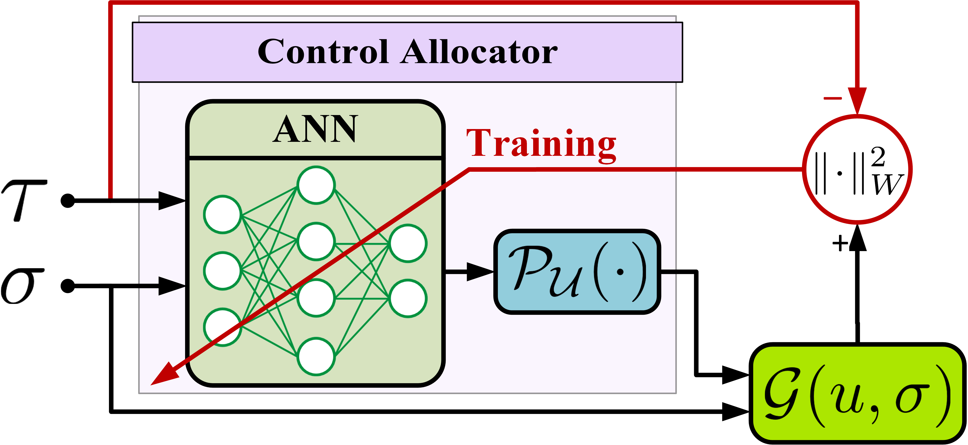
Figure 3: ANN Training Architecture

In many practical scenarios, control allocation is used as much more than just distribution of control commands. It is also employed for reconfiguration in the occurrence of faults [2], and for prioritization of control effectors [8]. In case of control effectors’ prioritization, daisy chaining approach is usually employed, which divides all effectors into multiple sets depending upon their priority. Then it is solved as sequential solution of small allocation problems for each set. In our ANN based approach this can be easily accomplished using multiple small ANNs for each set of effectors, and overall allocator can be obtained by appropriate stacking of these small networks.

For the case of reconfiguration based fault tolerance, there could be two possible approaches in our ANN based framework. (i) Separate ANN could be trained using standard approach for each failure case and switched during flight according to the occurrence of faults. (ii) A single network could be trained with an extra input which specifies all the fault scenarios. In this case training data would be the set of all possible faulty and healthy conditions.

IV Main Results

IV-A Performance of Control Allocator

There are multiple criterion to compare the performance of control allocation methods, most common are the Allocation Error and Volume Ratio of AMS of the method to actual AMS ($\mathcal{T}$) [3]. In literature allocation error is usually compared along a desired trajectory in $\mathcal{T}\times\mathcal{S}$ [5]. In this section, we present a slightly different yet more general definition of Maximum Allocation Error (MAE). It can not only be used to compare different allocation methods but also for stability & robustness analysis. Moreover, we define Volume Ratio for general nonlinear control allocation problem. Even tough for linear methods, tools are available to compute Volume Ratio [3] but for a general case such tools do not exit.

Given the effectiveness map $\mathcal{G}:\mathcal{U}\times\mathcal{S}\mapsto\mathcal{T}$, sets $\mathcal{U}$, $\mathcal{S}$, and $\mathcal{T}$, and a control allocator $\hat{u}:\mathcal{T}\times\mathcal{S}\mapsto\mathcal{U}$, we define following performance measures for this allocator. Here, it must be noted that for following definitions it is not necessary for the control allocator $\hat{u}$ to be a function; it could just be an algorithm. However, it needs to be a deterministic one.

Definition 3.

The Maximum Allocation Error (MAE) of an allocator $\hat{u}$ is defined as

$$\Delta_{\hat{u}}\triangleq\max_{\sigma\in\mathcal{S}}\max_{\tau\in\mathcal{T}_{\sigma}}\Big{\|}\mathcal{G}\left(\mathcal{P}_{\mathcal{U}}\left(\hat{u}(\tau,\sigma)\right),\sigma\right)-\tau\Big{\|}_{1}$$ (14)

where $\|\cdot\|_{1}$ represents 1-norm.

Definition 4.

The $pointwise$ AMS of an allocator $\hat{u}$ can be defined as

$$\mathcal{T}^{\hat{u}}_{\sigma}\triangleq\mathcal{G}\left(\mathcal{P}_{\mathcal{U}}\left(\hat{u}(\mathcal{T}_{\sigma},\sigma)\right),\sigma\right),\quad\forall\sigma\in\mathcal{S}$$ (15)

and similar to Definition 1, the total or complete AMS of an allocator $\hat{u}$ is defined as, $\mathcal{T}^{\hat{u}}\triangleq\bigcup_{\sigma\in\mathcal{S}}\mathcal{T}^{\hat{u}}_{\sigma}$.

Definition 5.

The Volume Ratio of allocator $\hat{u}$ is defined as the ratio of volume of AMS of allocator and volume of actual AMS. This can be written as

$$\mathcal{V}^{\hat{u}}\triangleq\min_{\sigma\in\mathcal{S}}\left(\left.\displaystyle\int_{\mathcal{T}^{\hat{u}}_{\sigma}}\mathrm{d}\tau\middle/\displaystyle\int_{\mathcal{T}_{\sigma}}\mathrm{d}\tau\right.\right)$$ (16)

Now, let’s consider practical aircraft control allocation problem, where $\mathcal{G}$ is in general piecewise linear function. Using this property in our ANN based allocation scheme yields following results:

Theorem 1.

For piecewise linear $\mathcal{G}$, and ANN based allocator with only piecewise-linear activations (e.g. ReLU), and hyper-cubical input set $\mathcal{U}=\{u\in\mathbb{R}^{m}|u_{min}\leq u\leq u_{max}\}$, the following holds:

1. The cost of (14) is also a piecewise linear function.

2. The solution of (14) can only be at the boundary of polytopes which divides the whole domain into finite regions and cannot be in interior of any of these polytopes.

3. If there are $\mathcal{N}$ polytopic regions for $\mathcal{G}\left(\mathcal{U},\sigma\right)$ or $\mathcal{G}\left(\mathcal{P}_{\mathcal{U}}\left(\hat{u}(\mathcal{T}_{\sigma},\sigma)\right),\sigma\right)$, $\forall\sigma\in\mathcal{S}$ (a fixed $\sigma\in\mathcal{S}$), and $\mathcal{T}_{i}$ being the AMS (point-wise AMS) of $i$th region, then $\mathcal{T}_{i}$ is a convex polytope for all $i\in[1,\mathcal{N}]$, complete AMS (complete point-wise AMS) can be written as

   $$\mathcal{T}=\bigcup_{i\in[1,\mathcal{N}]}\mathcal{T}_{i}$$ (17)

Proof.

To prove the first statement, with hyper-cubical input set $\mathcal{U}$, since $\mathcal{P}_{\mathcal{U}}(u)=\operatorname{sat}(u)\triangleq\min(\max(u,u_{min}),u_{max})$, therefore, $\mathcal{P}_{\mathcal{U}}$ is piecewise linear. Each layer of an ANN can be written as $a_{i}=\phi(\Theta_{i}a_{i-1}+b_{i})$ and since activation $\phi$ is assumed to be piecewise linear, so the complete ANN is piecewise linear. Moreover, the cost is 1-norm, which is defined as $\|x\|_{1}=|x_{1}|+|x_{2}|+\cdots+|x_{k}|$, it is also, piecewise linear. Now, recalling that any combination of piecewise linear functions is also a piecewise linear function completes the proof of the first statement.
For second and third statement, consider a single region (polytope) of the domain over which the cost is an affine function of inputs. The optimum (either maximum or minimum) of the function over the region cannot be in its interior, thus it must be on the boundary. Each region being a convex set when operated by an affine function results in a convex polytope (point-wise AMS). Therefore, complete AMS would be union of all these point-wise AMS of each region. ∎

Even though the above discussed theorem provides results of fundamental importance, its practical implementation is still being researched.

1. Given any two piecewise-linear functions, currently the authors have not been able to find an algorithm to determine the regions over which their composition is piecewise linear.

2. Given $n$ convex polytopes $T_{i},i\in[1,n]$, the volume of their union can be computed by inculsion-exculsion formula, but its computational cost is of order of $\mathcal{O}(n!)$. Another approach is to use the following identity:

   $$\mathcal{V}\left(\mathcal{T}\right)=\mathcal{V}\left(\mathcal{C}\right)-\mathcal{V}\left(\bigcap_{i\in[1,n]}\mathcal{C}\setminus\mathcal{T}_{i}\right)$$ (18)

   where $\mathcal{V}(\cdot)$ represent volume, $\mathcal{T}=\bigcup_{i\in[1,\mathcal{N}]}\mathcal{T}_{i}$, and $\mathcal{C}=\mathrm{Conv}\left(\mathcal{T}\right)$ represents convex hull. The second term in Eq. (18), though is usually very small in magnitude as compared to first one, but requires a lot of computational power.

In the upcoming section of this paper, we have used global optimization techniques for computation of MAE and Monte-Carlo based method for Volume Ratio estimation.

IV-B Closed Loop Stability Analysis

Consider a system of the following form:

$$\dot{x}=f(x)+B(x)\overbrace{\mathcal{G}(u,\sigma(x))}^{\tau}$$ (19)

where $x\in\mathcal{X}\in\mathbb{R}^{k}$ is the state vector, $u\in\mathcal{U}\subseteq\mathbb{R}^{n}$ is the true control input, $\tau\in\mathcal{T}\subseteq\mathbb{R}^{m}$ is the virtual control input, $\mathcal{G}:\mathcal{U}\times\mathcal{S}\mapsto\mathcal{T}$ is control effectiveness, $B:\mathcal{X}\mapsto\mathbb{R}^{k\times m}$ is a matrix with rank $m$, and $\sigma:\mathcal{X}\mapsto\mathcal{S}$ is a function of state; usually, it would be a subset of all states. Let’s assume from a control design technique that we have a virtual control law $\tau=\mathcal{P}_{\mathcal{T}_{\sigma(x)}}(k(x))$, which gives the ideal closed-loop system

$$\dot{x}=f(x)+B(x)\mathcal{P}_{\mathcal{T}_{\sigma(x)}}(k(x))$$ (20)

After incorporating control allocator $\hat{u}$, we get the following actual closed-loop system:

$$\dot{x}=f(x)+B(x)\mathcal{G}\left(\mathcal{P}_{\mathcal{U}}\left(\hat{u}(k(x),\sigma)\right),\sigma\right)$$ (21)

The basic idea of the following result is to treat the allocation error as non-vanishing but bounded perturbation at the input.

Theorem 2.

Let the origin ($x=0$), be an asymptotically stable (AS) equilibrium of the ideal closed-loop system (20), and let $V(x)$ be its Lyapunov function which satisfies

$$\begin{split}\alpha_{1}\left(\left\|x\right\|\right)\leq V(x)&\leq\alpha_{2}\left(\left\|x\right\|\right)\\ \left[\dfrac{\partial V}{\partial x}\right]^{\top}\left[f(x)+B(x)\mathcal{P}_{\mathcal{T}_{\sigma(x)}}(k(x))\right]&\leq-\alpha_{3}\left(\left\|x\right\|\right)\\ \left\|\left[\dfrac{\partial V}{\partial x}\right]^{\top}B(x)\right\|&\leq\alpha_{4}\left(\left\|x\right\|\right)\end{split}$$ (22)

$\forall\,x\in\mathcal{D}$, where $\mathcal{D}=\{x\in\mathcal{X}\mid\|x\|\leq r\}$, and $\alpha_{1},\alpha_{2},\alpha_{3},\alpha_{4}$ are class $\mathcal{K}$ functions. Suppose that the MAE satisfies

$$\Delta_{\hat{u}}\leq\theta\dfrac{\alpha_{3}\circ\alpha_{2}^{-1}\circ\alpha_{1}(r)}{\alpha_{4}(r)},\quad\forall\,x\in\mathcal{D},\,0<\theta<1$$ (23)

Then, $\forall\,\|x(t_{0})\|\leq\alpha_{2}^{-1}\circ\alpha_{1}(r)$ the solution $x(t)$ of actual closed-loop (21) satisfies

$$\|x(t)\|\leq\beta(\|x(t_{0})\|,t-t_{0}),\quad\forall\,t_{0}\leq t\leq t_{0}+T$$ (24)

and

$$\|x(t)\|\leq\rho(r),\quad\forall\,t\geq t_{0}+T$$ (25)

for some class $\mathcal{KL}$ function $\beta$, and some finite $T$, where $\rho$ is class $\mathcal{K}$ function and is defined as

$$\rho(r)=\alpha_{1}^{-1}\circ\alpha_{2}\circ\alpha_{3}^{-1}\left(\frac{\Delta_{\hat{u}}}{\theta}\alpha_{4}(r)\right)$$ (26)

Proof.

For simplifying notations, in this proof we have used $\mathcal{G}=\mathcal{G}\left(\mathcal{P}_{\mathcal{U}}\left(\hat{u}(k(x),\sigma)\right),\sigma\right)$, $\tau=\mathcal{P}_{\mathcal{T}_{\sigma(x)}}(k(x))$, and $\|\cdot\|_{k}$ as $k$-norm. Using $V(x)$ as Lyapunov function for actual closed-loop (21) we get,

$$\begin{split}\dot{V}(x)&=\left[\dfrac{\partial V}{\partial x}\right]^{\top}\left[f(x)+B(x)\mathcal{G}\right]\\ &=\left[\dfrac{\partial V}{\partial x}\right]^{\top}\left[f(x)+B(x)\tau+B(x)(\mathcal{G}-\tau)\right]\\ &\leq-\alpha_{3}(\|x\|)+\alpha_{4}(\|x\|)\|\mathcal{G}-\tau\|\\ &\leq-\alpha_{3}(\|x\|)+\alpha_{4}(\|x\|)\|\mathcal{G}-\tau\|_{1},\quad\because\|\cdot\|_{2}\leq\|\cdot\|_{1}\\ &\leq-\alpha_{3}(\|x\|)+\alpha_{4}(\|x\|)\Delta_{\hat{u}}\\ &\leq-(1-\theta)\alpha_{3}(\|x\|)-\theta\alpha_{3}(\|x\|)\\ &\qquad{}+\alpha_{4}(\|x\|)\Delta_{\hat{u}},\qquad\qquad 0<\theta<1\\ &\leq-(1-\theta)\alpha_{3}(\|x\|),\quad\forall\,\|x\|\geq\alpha_{3}\left(\frac{\Delta_{\hat{u}}}{\theta}\alpha_{4}(\|x\|)\right)\\ \end{split}$$

Applying Theorem 4.18 of [27] completes the proof. ∎

Remark.

It should be noted that though the above results have been presented for a case of static controller $k(x)$, the same results can be applied to any continuous dynamic or observer based controller, even with multi-loop control architecture. First step in such a case would be to write the complete closed-loop system in the form of Eq. (21), where $x$ represents all states (system, controller, observer - combined). Then this result can be applied directly.

V Aircraft Control Allocation: An Example

V-A Aircraft Specifications

In this work we have used aerodynamic model of a small-scale tailless flying wing aircraft. The comprehensive specifications of the aircraft can be found in [24, 23].

The aircraft under discussion has six trailing edge surfaces ($\delta_{1},\cdots,\delta_{6}$) and two (left/right) pairs of clamshell surfaces ($\delta_{7U},\delta_{7L}$ and $\delta_{8U},\delta_{8L}$). Deflection of trailing edge surfaces in downward direction is considered to be positive whereas in upward direction it is considered to be negative.

TABLE I: Saturation limits of control surfaces

Surface	Min.	Max.
$\delta_{e}$	-20	20
$\delta_{7U}$ & $\delta_{8U}$	0	40
$\delta_{7L}$ & $\delta_{8L}$	-40	0

In total this aircraft has ten control surfaces. Any combination of these surfaces can be used to maneuver the aircraft. For this case, the authors have studied all trailing edge surfaces ($\delta_{1},\cdots,\delta_{6}$) as a single elevator ($\delta_{e}$). This results in five independent control surfaces to be considered for control allocation problem. The saturation limits of the control surfaces are given in Table I.

V-B Results & Discussion

Training data was randomly generated using Latin Hypercube sampling. A data set comprising of 0.1 million data point was generated. This dataset was split with a ratio of 0.7, 0.15, 0.15 into training, validation, and test data sets, respectively. Keras API in Pthyon was used to design and train the ANNs. Adam optimizer was utilized as the optimization scheme, where the learning rate was initially kept as 0.005. The first and second moments were maintained at 0.9 and 0.999, respectively. Mean Squared Error (MSE) was kept as the loss function, while Root Mean Squared Error (RMSE) and R-squared ($R^{2}$) values were kept as metrics to measure the performance of the networks. Rectified Linear Unit (ReLU) was used as the activation function in all hidden layers due to its computational simplicity and effectiveness in handling of vanishing gradients. It should be noted that the theoretical results discussed in section IV-A focused on piece-wise linear activation e.g., ReLU. Every network was trained for 50 epochs with the data being fed to the network in multiple batches of 128 samples. Validation losses were also monitored simultaneously, and the learning rate was automatically reduced by a factor of 10% if the validation loss did not improve after a patience period of 5 epochs.

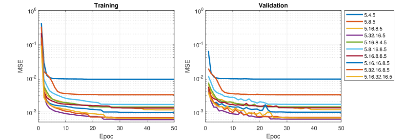
Figure 4: History of MSE for Training & Validation Sets

Figure 5: History of Learning Rate During Training

Fig. 4 shows MSE history of training and validation sets. It can be seen that for all network configurations the MSE settles down in a straight line. This depicts that the network has fully learnt the data set and training it for more epochs would not improve its performance. Fig. 5 shows the learning rate history. It can be seen that for later epochs the learning rate has dropped down to almost zero which validates the previous claim that the network has fully trained.

TABLE II: Comparison of Different ANN Architectures

Control Allocator		No. of Parameters	MSE	$R^{2}$	MAE ($\Delta_{\hat{u}}$)
ANN Based	5.4.5	59	$9.166\times 10^{-3}$	0.9907	0.0300
	5.8.5	103	$3.096\times 10^{-3}$	0.9969	0.0286
	5.16.8.5	287	$\pagecolor{blue!10}{\color[rgb]{0,0.5,0}\mathbf{1.106\times 10^{-3}}}$	0.9989	0.0226
	5.16.8.4.5	303	$1.327\times 10^{-3}$	0.9987	0.0234
	5.16.8.8.5	359	$1.265\times 10^{-3}$	0.9987	0.0232
	5.8.16.8.5	383	$1.587\times 10^{-3}$	0.9984	0.0266
	5.16.16.8.5	559	$9.439\times 10^{-4}$	0.9990	0.0215
	5.32.16.5	815	$5.926\times 10^{-4}$	0.9994	0.0185
	5.32.16.8.5	911	$6.589\times 10^{-4}$	0.9993	0.0207
	5.16.32.16.5	1263	$6.270\times 10^{-4}$	0.9994	0.0185
QP Based (Polynomial Model)		552	${}-{}$	${}-{}$	0.0326

The first column in Table II depicts different architectures of the ANNs studied. For example, the first entry ‘5.4.5’ means that the network has five inputs and five outputs and a single hidden layer comprising of four neurons. Similarly, ‘5.32.16.5’ means that inputs and outputs remain five. However, this architecture has two hidden layers with 32 and 16 neurons, respectively. Out of five inputs for each network; first three are desired moments and last two are angle of attack ($\alpha$) and sideslip angle ($\beta$). Output are deflection of five control surfaces ($\delta_{e},\delta_{7U},\delta_{7L},\delta_{8U}$, and $\delta_{8L}$). The second column depicts the number of parameters required to implement ANN based control allocator on flight computer. The succeeding two columns depict MSE and $R^{2}$ of test data set. The last column represents the Maximum Allocation Error (MAE) as defined in section IV-A. It was computed through MATLAB’s GlobalSearch function while using fmincon as its local solver.

These different network architectures were compared to traditional quadratic programming (QP) based affine control allocation scheme. This method requires local slopes and offsets at each sampling instant, which in turn needs an onboard model of control effectiveness ($\mathcal{G}(u,\sigma)$). These slopes and offsets were obtained through a polynomial based model which is a standard practice.

Observing the values obtained of MSE and $R^{2}$ it can be noted that with increase in hidden layers and number of neurons the network performance is improved. It is also observed that the network performance of ‘5.16.8.5’ is best suited in our opinion, as there is no substantial betterment in performance with increasing the number of hidden layers and the number of neurons after that. With small number of parameters and decent performance (MSE, $R^{2}$ and MAE), it is a logical choice for network architecture. This selected architecture has smaller allocation error, while lesser number of parameters are required than the traditional scheme.

The desired moment vector is applied in terms of the pre-defined trajectories of moment coefficients $C_{l}$, $C_{m}$ and $C_{n}$, which correspond to the helical path with radius 0.003. The angle of attack ($\alpha$) is varied from 0 deg (at 0 sec) to 8 deg (at 1 sec), and sideslip angle ($\beta$) is varied from -12 deg (at 0 sec) to 12 deg (at 1 sec). Thus, the control allocation algorithm is evaluated for almost complete variation of control interaction with respect to deflections, angle of attack and sideslip angle. Fig. 6 depicts the moments generated by different allocation schemes. It is noticed that the network selected follows the desired moments quite closely. Fig. 7 shows that both ANN based allocator and traditional method have similar (very small) allocation errors. Even though both methods have similar performance however proposed ANN based scheme is preferable because it requires less data storage. It is also computationally much efficient than the traditional method as it only requires few matrix operations, whereas the standard method requires solving of a quadratic program at each sampling instant. Table III shows average time taken by both methods to allocate a single vector of desired moments. It can be seen that the ANN based scheme is much more efficient. However, it must be noted that these values are from MATLAB’s tic-toc routine on a normal laptop. So, in actual onboard implementation, values might differ, but the relative difference would remain of similar order.

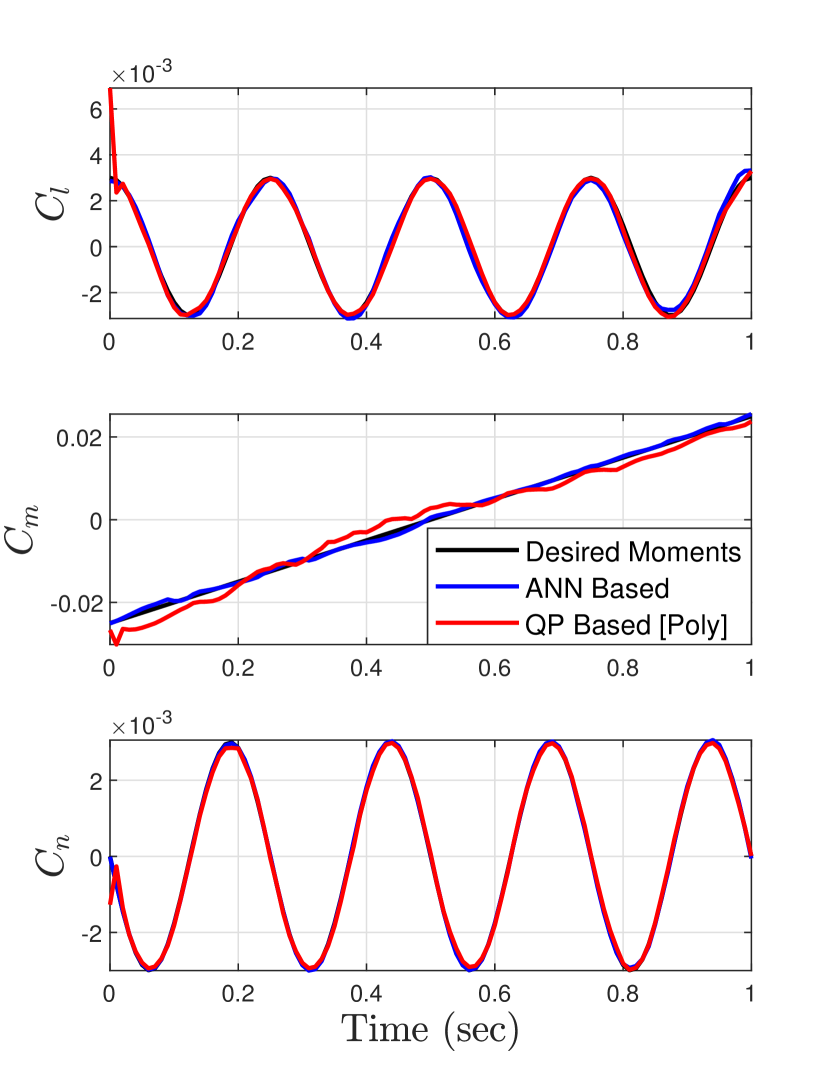
Figure 6: Comparison of Performance

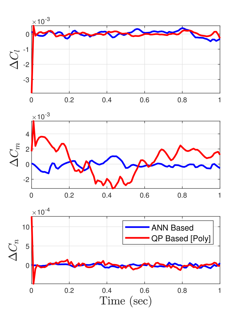
Figure 7: Comparison of Allocation Error

TABLE III: Average Execution Time Comparison

Method	Time [msec]
ANN Based	0.143
QP Based [Poly]	15.68

VI Conclusion

In this research work, a general nonlinear control allocation problem was posed in a different perspective, that is to seek a function which maps desired moments to control effectors. This view of control allocation is similar to pseudo-inverse methods for linear allocation problems, but differs with optimization based methods for either linear or nonlinear allocation problems, which try to find control effector commands for a given desired moments vector. Allocation problem was converted to a machine learning problem and training methodologies for different types of allocation problems were presented, e.g. effectors prioritization, fault tolerance, reconfiguration etc.

Two important results for nonlinear control allocation problem were presented in this work. Firstly, computational issues of performance parameters for piecewise linear effectiveness functions with ANN based allocators were discussed. Secondly, the conditions of closed loop stability, with allocator in the loop, in terms of maximum allocation error, were presented. However, there are a few future research avenues which need to be further explored in regard to the development of efficient algorithms for detailed performance analysis of different allocators, e.g., volume computation of union of convex polytopes and the calculation of domain partitions for composition of piecewise linear functions.

Later, to demonstrate the efficacy of the proposed allocator, the results were compared with those obtained from standard QP based method with polynomial model. It was shown to have similar performance with reduced number of parameters required and with much less computational cost. The results also portrayed that the run time for the proposed scheme of ANN based control allocator was less than standard QP based method by an order of magnitude.

Hafiz Zeeshan Iqbal Khan received his BS degree magna cum laude in Aerospace Engineering, from Institute of Space Technology, Islamabad, Pakistan, in 2015, with honors and President of Pakistan gold medal. He received his MS degree summa cum laude in Aerospace Engineering specializing in Guidance, Navigation & Control, from Institute of Space Technology, Islamabad, Pakistan, in 2019, with honors. His main research interests include dynamics & control of aerospace vehicles, robust control, nonlinear control, geometric control, and machine learning.

Surrayya Mobeen received her BS degree in Aerospace Engineering, from Institute of Space Technology, Islamabad, Pakistan, in 2015. She received her MS degree in Aerospace Engineering specializing in Guidance, Navigation & Control, from Institute of Space Technology, Islamabad, Pakistan, in 2019. Currently, she is working as a researcher at Institute of Space Technology, Islamabad, Pakistan. Her main research interests include rotorcraft dynamics, nonlinear control, artificial intelligence, fault tolerant control, and estimation.

Jahanzeb Rajput received the B.E. degree in Electronics Engineering from Mehran University of Engineering and Technology, Jamshoro, Pakistan, in 2005. He received the M.S. degree in Control Engineering from University of Engineering and Technology, Lahore, Pakistan, in 2007. He received the Ph.D. degree in Navigation, Guidance and Control from Northwestern Polytechnical University, Xi’an, China, in 2016. His main research interests include nonlinear control, control allocation, fault-tolerant control, reconfigurable control, modeling, identification and simulation.

Jamshed Riaz [HI(M), SI(M), PoP] received his BS degree in Aerospace Engineering from PAF College of Aeronautical Engineering, Karachi (now at Risalpur), Pakistan, in 1976. He received his MS and PhD degrees in Aerospace Engineering from Georgia Institute of Technology, USA, in 1992. He was on the winning team of McDonnell Douglas sponsored Light Utility Helicopter Competition in 1990. Since 2013, he has been a Professor at Institute of Space Technology, Islamabad, Pakistan. His current research interests include flight dynamics, rotorcraft dynamics and automatic control.

References

- [1] K. M. Dorsett and D. R. Mehl, “Innovative control effectors (ice),” Lockheed Martin Tactical Aircraft Systems Fort Worth TX, Tech. Rep., 1996.
- [2] H. Z. I. Khan, J. Rajput, and J. Riaz, “Reconfigurable control of a class of multicopters,” in European Control Conference (ECC), 2020, pp. 1632–1637.
- [3] W. Durham, K. A. Bordignon, and R. Beck, Aircraft control allocation. John Wiley & Sons, 2017.
- [4] M. W. Oppenheimer, D. B. Doman, and M. A. Bolender, Control Allocation, 2nd ed., ser. The Control Handbook. CRC Press, 2011, book section 8.
- [5] W. C. Durham, “Constrained control allocation - three-moment problem,” Journal of Guidance, Control, and Dynamics, vol. 17, no. 2, pp. 330–336, 1994.
- [6] K. A. Bordignon, “Constrained control allocation for systems with redundant control effectors,” Ph.D. dissertation, Virginia Polytechnical Instittute and State University, 1996.
- [7] M. Bodson, “Evaluation of optimization methods for control allocation,” Journal of Guidance, Control, and Dynamics, vol. 25, no. 4, pp. 703–711, 2002. [Online]. Available: https://doi.org/10.2514/2.4937
- [8] J. M. Buffington and D. F. Enns, “Lyapunov stability analysis of daisy chain control allocation,” Journal of Guidance, Control, and Dynamics, vol. 19, no. 6, pp. 1226–1230, Nov. 1996. [Online]. Available: https://doi.org/10.2514/3.21776
- [9] J. F. Buffington, “Modular control law design for the innovative control effectors (ice) tailless fighter aircraft configuration 101-3,” US Air Force Research Lab Wright-Patterson AFB OH, Tech. Rep., 1999.
- [10] D. Enns, “Control allocation approaches,” in Guidance, Navigation, and Control Conference and Exhibit, ser. Guidance, Navigation, and Control and Co-located Conferences. American Institute of Aeronautics and Astronautics, 1998. [Online]. Available: https://doi.org/10.2514/6.1998-4109
- [11] T. A. Johansen and T. I. Fossen, “Control allocation — a survey,” Automatica, vol. 49, no. 5, pp. 1087–1103, 2013.
- [12] M. A. Niestroy, K. M. Dorsett, and K. Markstein, “A tailless fighter aircraft model for control-related research and development,” in AIAA Modeling and Simulation Technologies Conference, ser. AIAA SciTech Forum. American Institute of Aeronautics and Astronautics, Jan. 2017. [Online]. Available: https://doi.org/10.2514/6.2017-1757
- [13] J. Rajput, Q. Xiaobo, and H. Z. I. Khan, “Nonlinear control allocation for interacting control effectors using bivariate taylor expansion,” in 5th International Conference on Control, Decision and Information Technologies (CoDIT), 2018, pp. 352–357.
- [14] V. L. Poonamallee, S. Yurkovich, A. Serrani, and D. B. Doman, “A nonlinear programming approach for control allocation,” in Proceedings of the 2004 American Control Conference, vol. 2, 2004, pp. 1689–1694 vol.2.
- [15] M. A. Bolender and D. B. Doman, “Nonlinear control allocation using piecewise linear functions,” Journal of Guidance, Control, and Dynamics, vol. 27, no. 6, pp. 1017–1027, Nov. 2004. [Online]. Available: https://doi.org/10.2514/1.9546
- [16] ——, “Nonlinear control allocation using piecewise linear functions: A linear programming approach,” Journal of Guidance, Control, and Dynamics, vol. 28, no. 3, pp. 558–562, May 2005. [Online]. Available: https://doi.org/10.2514/1.12997
- [17] Y. Luo, A. Serrani, S. Yurkovich, M. W. Oppenheimer, and D. B. Doman, “Model-predictive dynamic control allocation scheme for reentry vehicles,” Journal of Guidance, Control, and Dynamics, vol. 30, no. 1, pp. 100–113, Jan. 2007. [Online]. Available: https://doi.org/10.2514/1.25473
- [18] B. C. Csáji, “Approximation with artificial neural networks,” Master’s thesis, Faculty of Sciences, Etvs Lornd University, Hungary, 2001.
- [19] R. Grogan, W. Durham, and R. Krishnan, “On the application of neural network computing to the constrained flight control allocation problem,” in Guidance, Navigation, and Control Conference, ser. Guidance, Navigation, and Control and Co-located Conferences, no. 0. American Institute of Aeronautics and Astronautics, Aug. 1994. [Online]. Available: https://doi.org/10.2514/6.1994-3644
- [20] M. Chen, “Constrained control allocation for overactuated aircraft using a neurodynamic model,” IEEE Transactions on Systems, Man, and Cybernetics: Systems, vol. 46, no. 12, pp. 1630–1641, 2016.
- [21] H. Huan, W. Wan, C. We, and Y. He, “Constrained nonlinear control allocation based on deep auto-encoder neural networks,” in European Control Conference (ECC), 2018, pp. 1–8.
- [22] P. S. de Vries and E.-J. Van Kampen, “Reinforcement learning-based control allocation for the innovative control effectors aircraft,” ser. AIAA SciTech Forum, no. 0. American Institute of Aeronautics and Astronautics, Jan. 2019. [Online]. Available: https://doi.org/10.2514/6.2019-0144
- [23] X. Qu, W. Zhang, J. Shi, and Y. Lyu, “A novel yaw control method for flying-wing aircraft in low speed regime,” Aerospace Science and Technology, vol. 69, pp. 636–649, 2017. [Online]. Available: http://www.sciencedirect.com/science/article/pii/S1270963817305539
- [24] J. Rajput, Z. Weiguo, and S. Jingping, “A backstepping based flight control design for an overactuated flying wing aircraft,” in 10th Asian Control Conference (ASCC), 2015, pp. 1–6.
- [25] I. Goodfellow, Y. Bengio, A. Courville, and Y. Bengio, Deep learning. MIT press Cambridge, 2016, vol. 1, no. 2.
- [26] S. Haykin, Neural networks and learning machines, 3rd ed. Pearson Education, 2010.
- [27] H. K. Khalil, Nonlinear Systems, ser. Pearson Education. Prentice Hall, 2002.