Comparison of spin-correlation and polarization variables of spin density matrix for top quark pairs at the LHC and New Physics implications
Abstract
Precise determination of top-quark pairs is an essential tool for understanding the overall consistency of the standard model (SM) expectations, understanding limited New Physics (NP) models, through spin-spin correlation and polarization parameters, and has a critical impact on the analyses strategies at upcoming LHC programs. In this work, we review and discuss various state-of-the-art Monte Carlo (MC) methodologies as MadGraph5_aMC@NLO, Sherpa, Powheg-Box and Pythia8, which are Matrix Element (ME)Parton Shower (PS) matching generators including a complete set of spin correlation and polarization in top quark pair production with dileptonic final states. This is the first such study that not only compares the effects of different MC event generator approaches on spin density matrix elements and polarization parameters, but also investigates the effects of leading order (LO) and next-to-leading order (NLO) accuracy in QCD, and electroweak (EW) corrections via Sherpa. Moreover, as a continuation of the work, the prospects for possible NP scenarios through top-quark spin-spin correlation and polarization measurements for Supersymmetry (R parity conserved and violated models) and Dark Matter (top quarks associated mediator) models during upcoming LHC runs are briefly outlined. We find that all SM MC predictions for the defined set of variables are generally consistent with the experimental data and theoretical predictions within the uncertainty variations. Besides, for the distributions of the , laboratory-frame observables ( and ) and the observables generated by parity (P) and charge-parity (CP) conserving interactions, we conclude some clues that the considered signals and beyond may well be separated from experimental data and located above the SM predictions.
Keywords:
Top Quark, Hadronic Colliders, MC Simulations1 Introduction
Top quark pair production is still one of the most critical process in collider physics today. As the heaviest known fundamental particle in the standard model (SM), the top-quark provides a unique opportunity to understand the critical behaviour of Yukawa coupling close to unity, making it a more important subject for beyond standard model (BSM) scenarios and in discussions of the stability of the SM universe. Top-quark properties is therefore an increasingly important input to many analyses in the following LHC runs. Understanding higher order effects together with electroweak corrections to top-quark processes play a crucial role in precision measurements, such as spin-correlation and polarization of top-quark pairs 0a ; 0b ; 0c ; 0d ; 0e ; 0f ; 0g , and many other unknown BSM signals, such as supersymmetry and effective field theory (EFT) models 0h ; 0i . More generally top quarks are unavoidable facts in BSM searches, both as signal objects and for backgrounds (e.g. as a source of leptons and b quarks).
Monte Carlo (MC) event generators are critical tools for the analysis and interpretation of LHC analyses in today research 0j ; 0j1 ; 0j2 . In particular, detailed aspects of the final states produced in individual processes, such as top-quark pair production, are to be required advanced calculations 0k ; 0k1 ; 0k2 . Top-quark pair production comprise for example the contribution of higher order matrix element calculations with multiple partons, the evaluation of parton shower and fragmentation, parton shower matching selection efficiencies, and the extrapolation of cross sections to the full phase space. In this manner, considering recent developments in higher-order perturbative corrections, in particular in QCD, but also in QED and in the electroweak sector, comparison studies of MC approaches are a critical subject that makes some precision measurements and data interpretation more visible. Based on a high level of calculation - studied with LHC data - these contributions allow for both the realistic simulation of top-quark pairs precision measurements and the possible understanding of BSM signals. Thus, complex contributions of various MC approaches to experimental objects and variables are a vital subject of collider-based particle physics studies.
In the following sections, we provide an overview of the up-to-date top-quark pairs hadron level production with various MC methodologies, above all, we will try to stress the main motivation of the extended discussion of a spin density matrix for the top pair system existing consistency and controversies concerning interpretation of the LHC measurements, as well as the sources of theory uncertainty. All in all, we review the precision measurement of spin density matrix of top quark-pairs; discuss the NP ambiguity; and the main strategies to measure spin-correleation and polarization top-quark pairs will be presented. The interpretation of 22 different measurements and the theoretical uncertainties will be discussed while conclusion will contain some final remarks for future LHC runs.
As it is known, even though the SM is a theory that has been proven many times by various tests, it has problems that it cannot solve, such as hierarchy problem and dark matter (DM). Supersymmetry (SUSY) as an extension of the SM could help to elucidate these both problems by introducing additional particles (e.g. bosonic superpartner of the top quark (stop, )) that cancel large quantum corrections to the Higgs boson squared mass in the SM and feasible DM candidates. Due to the central role of the top quark in interaction with these hypothetical particles, collaborations like ATLAS and CMS try to measure top quark properties accurately to find these signals in the experiment. Searches for stop and DM candidate particles concentrate generally on high missing transverse energy region stem from undetected lightest SUSY particles (LSP), as a decay product of , and DM candidate particles. With these studies, most of the high region, even low , was excluded by ATLAS and CMS Collaborations 1a ; 1b ; 0e ; 1d . In the last step of the study, we will focus on the interpretation of SUSY and DM signals in low region, which are studied with generic searching methods, by measuring precisely. The signals are based on simplified models, which are the similar topology with the models in the ref. 1a , of stop pair production and of top quark pair production in associated with fermionic DM candidate particles. In the SUSY signal, in figure 1(a), a pair of stop decays an on-shell top quark and an LSP, in this case neutralino , which is stable for this simplified model. In order to investigate the deviations of the signal from SM , one mass point which is GeV for and GeV for will be used. An alternative dark matter signal in figure 1(b) include a scalar or pseudoscalar spin-0 mediator decayed into fermionic DM particles and an associated top quark pair. The coupling strengths of the DM-mediator and the mediator-SM fermions are assumed to be equal to one in the simplified model. Additionally, in this analysis, the scenario with GeV and GeV will be focused.
In the above models, we focused on a small mass point to ensure low . However, the additional model of R-Parity 1e violating (RPV) SUSY provides more mass points to study for low due to the decaying . The decays into three quarks with the help of a trilinear Yukawa coupling between quarks and superpartner of quarks (squark) 1f . In this study, the production chain includes a pair decaying into a and a as shown in figure 1(c), and the goes into three light flavor quarks , , as considered in ref. 1g . For the RPV SUSY scenario, masses up to GeV have been excluded, by CMS Collaboration 1g , at confidence level with a maximum observed local significance of for GeV.
This paper structured as follows: in the next section, we describe the MC data samples and the CMS data used in the analysis, with generator settings for all and signal samples. In section 3, we introduce the set of observables of spin correlation and polarization in top quark pair production by using decomposition of spin density matrix. In section 4, we present our results for the differential distributions of the observables. The results are divided into two parts as the comparison of different MC event generator configurations on the distributions of the observables of events and the investigation of behaviours of signals having different topology on the observables. Finally, our conclusions are given in section 5.
2 Event Samples and Data
A range of MC generators to provide predictions for top quark pair production and related BSM signal processes are used to investigate the effects of various approaches of MC generators on top pair spin correlation matrix and polarization variables and to assess the differences between BSM signals and top quark pairs.
A summary of the produced MC samples, describing various the SM top quark pair production processes and the possible signal scenarios, is shown in table 1. The table also lists details of the simulation samples used, including the matrix element (ME) event generator with the order of the calculation and the central parton distribution function (PDF) set, the parton shower (PS) and hadronization model, and the merging scheme used to remove the overlap between ME and PS.
| Process | ME PDF | ME generator | Order | PS and | Merging |
| (MEPS) | hadronization | scheme | |||
| NNPDF3.0 NLO | MG5_aMC@NLO | NLOLL | Pythia 8 | FxFx | |
| NNPDF3.0 LO | MG5_aMC@NLO | LOLL | Pythia 8 | MLM | |
| NNPDF3.0 NLO | Powheg-Box | NLOLL | Pythia 8 | Powheg | |
| NNPDF3.0 NLO | Sherpa 2 | NLO(EW)LL | CSShower | MEPS@NLO | |
| NNPDF3.0 LO | Sherpa 2 | LOLL | CSShower | MEPS@LO | |
| NNPDF3.1 LO | MG5_aMC@NLO | LOLL | Pythia 8 | MLM | |
| NNPDF3.1 LO | MG5_aMC@NLO | LOLL | Pythia 8 | MLM |
In all background and signal samples events are produced with a top quark mass of GeV. The nominal sample (with up to two additional matched partons included in the ME calculations) is simulated using MadGraph5_aMC@NLO (v2.6.7) b at NLO QCD accuracy. To evaluate the effects of different perturbative orders of the calculation, we have been used the samples generated with MadGraph5_aMC@NLO at LO accuracy as well. The parton showers are modelled using Pythia (v8.2.44) c with the default showering tunes at leading logarithmic (LL) accuracy. The matrix elements at LO and NLO are merged with the parton shower using the MLM d and the FxFx e merging scheme, respectively. In order to determine state-of-the-art theoretical approaches between the different methods in MC generators, two additional generator setups are incorporated in the analysis chain. Firstly, sample is generated using the Sherpa (v2.2.8) f generator with up to three extra partons at LO and NLO. The Sherpa, in production of events, employs Amegic++ g1 , Comix g and OpenLoops h ; i ; j (for one-loop amplitudes) in matrix elements calculation which are merged with CSShower k for parton showering (with LL accuracy) and hadronization by using the MEPS@NLO l ; m prescription. To match the ME and PS results, Sherpa and MadGraph5_aMC@NLO make use of the same normalization method, which is MC@NLO n . The other alternative sample is generated with Powheg (v2) o ; p ; q ; r including up to two extra matched partons at the ME level with NLO accuracy. The parton shower is employed by Pythia (v8.2.40) with GeV parameter of Powheg.
For all SM samples listed, the initial state partons are modeled with the NNPDF3.0 PDF set s ; t implemented by LHAPDF u . To determine the systematic uncertainties in predictions, uncertainties coming from PDF and scale variations are used as summed in quadrature. Parton distribution function uncertainties are evaluated by reweighting the samples generated by MadGraph5_aMC@NLO at LO and Sherpa for all setups using generator weights related with each of the variations given by NNPDF3.0, CT10 v and MMHT14 w PDF sets. Renormalization and factorization scale uncertainties are calculated using variations by a factor of two around the central scales which are equal to for MadGraph5_aMC@NLO and for Sherpa setup x , where is the transverse momentum of top quarks.
Signal samples of SUSY and RPV SUSY are simulated at LO with up to three and two additional partons, respectively, with MadGraph5_aMC@NLO (v2.4.2) interfaced to Pythia (v8.2.40) for parton showering and hadronization using the MLM merging scheme. For the SUSY sample in figure 1(a), the masses of the and the will be considered as GeV and GeV. On the RPV SUSY side, the masses of the and the are taken as GeV and GeV, respectively.
The other signal samples are top quark pairs associated with DM particles as shown in figure 1(b) which is included scalar or pseudoscalar mediators. The DM signal samples are simulated at LO including up to one additional parton with MadGraph5_aMC@NLO (v2.6.1) interfaced with the Pythia (v8.2.40) PS model using the MLM merging scheme. The masses of the and the will be considered as GeV and GeV. In all signal samples, NNPDF3.1 PDF set is used in ME calculation.
To assess the truth of the theoretical predictions, experimental measurements published by CMS Collaboration are directly used 0i . The CMS analysis unfolded the data to compare with parton level predictions at full phase space. In our analysis, the MC predictions have baseline selections compatible with the CMS analysis.
3 Spin Correlations on Top Quark Pairs
The total cross section for the top pair production at accelerator energy can be written as
| (1) |
by using factorization theorem. This theorem divides the total cross section into a short distance (hard) part and a long distance (soft) part, which is known as parton distribution function (PDF). The PDF determine the probability of the existence of a parton () in the hadron A (B) with a rate () of the longitudinal momentum of the hadron at the factorization scale . The partonic cross section involves the spin information of top quark and anti-quark. However the spin information of a top quark is not detectable because of short life time of it. In spite of the fact that the spin of an unstable particle produced in high energy reactions is no straightforwardly noticeable quantity, it is extremely helpful to present the idea of a spin density matrix z for the top pair system (2). The decay width of the top quark much smaller than its mass allows to use narrow width approximation (NWA) aa ; ab . Using NWA, the matrix element of the top pair production can be written as the trace of the production and the decay factors:
| (2) |
where is the spin density matrix of the on-shell top pair production and and are the decay spin density matrices of the polarized top quark and antiquark, respectively. To look at the spin properties of the top quark and antiquark, spin density matrix can be decomposed in the spin space of and .
| (3) |
Here, the first terms which are a 2x2 unit matrix and the Pauli matrices in the tensor products refer to top spin spaces, and second terms refer to anti-top.
While the function is related to the total cross section and the top quarks kinematic properties, and are 3-vectors that describe the polarizations of and in each direction, and 3x3 matrix that determine the spin correlation between top quark and antiquark.
As mentioned earlier, decay of the top quarks before hadronization allows to study the spins of them by looking at the angular distribution of the decay products. Top quarks decay almost to a boson and a bottom quark. The final states of the decay coming from boson can be a quark-antiquark pair or a lepton and a neutrino. The angular distribution of the top decay products with respect to the spin alignment of the top is given by
| (4) |
with the angle between the 3-momentum of decay product in the top rest frame and the direction of the top spin. is the spin analyzing power of . The spin analyzing power of the charged lepton is almost equal to which is maximum value. For a top antiquark, is minus sign of the top quark one. It does not change much at NLO QCD ac . To make use of high valued spin analyzing power, leptons have been used as a proxy for spins of top quarks and anti-quarks.
The functions and in equation (3) can be written as a linear combination of coefficient functions associated with an orthonormal basis. The basis in this analysis was chosen as the helicity basis as it gives more spin correlation compared to other alternatives as discussed in ref. 0c . This basis can be shown in figure 2. is described as helicity axis determined by the top quark direction in the center-of-mass (CM) frame. The direction indicates the direction of one of the incoming partons in the same frame. Using the directions and , the normal to the scattering plane and the direction perpendicular to in the scattering plane are given by and .
A redefinition of the and axes is necessitated owing to the Bose-Einstein symmetry of the initial state 0h . The reference axes and are described with above regularization as
| (5) |
Using the orthonormal basis, and are decomposed as
| (6) |
| (7) |
The coefficient functions , and which are functions of the partonic center of mass-energy and are related to some discrete symmetries such as parity (P) and charge-parity (CP), and they are summarized in table 2.
| Observable | Measured | Coefficient | Symmetries | |
| coefficient | function | |||
| polarization | P-odd, CP-even | |||
| P-odd, CP-even | ||||
| P-odd, CP-even | ||||
| P-odd, CP-even | ||||
| P-even, CP-even | ||||
| P-even, CP-even | ||||
| P-odd, CP-even | ||||
| P-odd, CP-even | ||||
| P-odd, CP-even | ||||
| P-odd, CP-even | ||||
| diagonal spin corr. | P-even, CP-even | |||
|---|---|---|---|---|
| P-even, CP-even | ||||
| P-even, CP-even | ||||
| cross spin corr. | P-even, CP-even | |||
| P-even, CP-odd | ||||
| P-odd, CP-even | ||||
| P-odd, CP-odd | ||||
| P-odd, CP-even | ||||
| P-odd, CP-odd | ||||
| P-even, CP-even | ||||
| lab. frame | ||||
According to table 2, the P- and CP-even coefficient functions (, , and ) can have large values due to the parity invariance of strong interaction. However, the presence of electroweak (EW) corrections can result in non-zero P-odd and CP-even coefficients ( and ). On the other hand, the coefficients produced by CP-violating interactions are close to zero in the SM. The approximate CP invariance of the SM limits the top and anti-top quarks to have the same polarization, so has a value of zero222See ref. 0h for further details..
After the equations (2) and (3), the normalized distribution for the two leptons final state can be written in the form of spin coefficients and direction of flight of the leptons. This can be simplified as the differential distribution of the cross-section. The cross section distribution for the double leptonic channel can be written as 0i
| (8) |
where is the angle between the direction of flight of the positively (negatively) charged lepton in the top quark (anti-quark) rest frame and a reference direction (). The coefficients and in (8) reflect the properties of the spin density components in (3). The elements of and matrices have the same discrete symmetry properties with related coefficient functions, see in table 2. To extract each coefficient separately one can reduce the double differential cross section in equation (8) to single differential distributions
| (9) |
| (10) |
| (11) |
| (12) |
where . In addition to eqs. (9), (10), four further observables with respect to modified axes and are calculated. Axes and for top quark are equal to and , respectively, while they are inverse for anti-top. Here is the difference in absolute values of the rapidities of top and anti-top quarks in the laboratory frame. The observables in modified axes may sensitive to the NP contributions 0h .
The opening angle , which is obtained by the inner product of the direction of flight of positively and negatively charged leptons in their own top quark rest frames, is taken into account as a useful spin correlation observable below. The analysis also involves two observables measured directly in the laboratory-frame. First one is , which is defined as but in the laboratory-frame. is the other observable measured in the laboratory-frame. It is the absolute azimuthal difference between the two charged leptons measured in the laboratory-frame. The observables measured in the laboratory-frame cannot be obtained from spin correlation or polarization observables, but they could have high precision in measurement and computation.
4 Results
In this section, the normalized differential distributions for the 22 observables mentioned in previous section are presented as a comparison of various MC approaches and experimental measurements published by the CMS Collaboration 0i . The physics objects in events predicted by MC generators are considered at generator-level. In that sense, objects come from MC history after decay but before hadronization. Last top quark in top quark decay chain as a top quark and first lepton after decay of W boson as a lepton are used in the calculations of observables. As leptons in dilepton events, prompt electrons and muons (not taus or decay products of taus) are taken into account.
Three different MC generators as MadGraph5_aMC@NLO, Sherpa and Powheg box at LO and NLO QCD accuracy used in the analysis. As in the CMS analysis 0i , the analysis with MC generators is in full phase space. As the nominal sample, we have been chosen the sample simulated by MadGraph5_aMC@NLO ME event generator at NLO interfaced with Pythia8 for the parton shower and fragmentation.
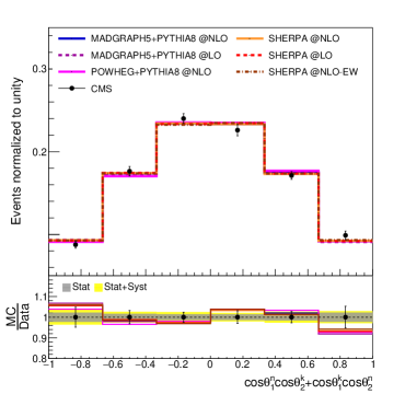
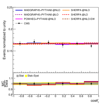
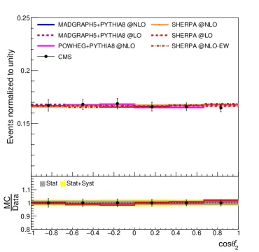
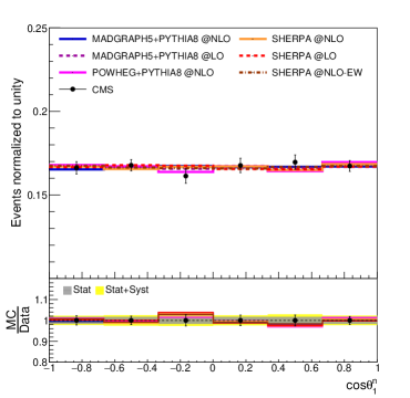
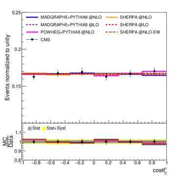
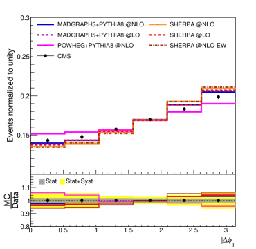
In figures 3-8, the differential distributions predicted by MadGraph5+Pythia8 at NLO is compared with MadGraph5+Pythia8 at LO accuracy, with Powheg+Pythia8 at NLO, with Sherpa at LO, and with Sherpa at NLO QCD accuracy and at NLO in QCD with EW correction. To check the compatibility with experiment, whole that theoretical predictions are compared with CMS measurements.
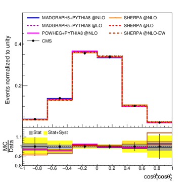
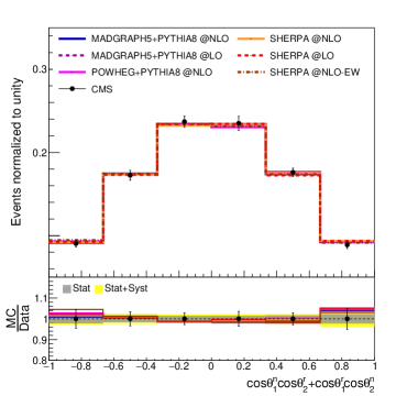
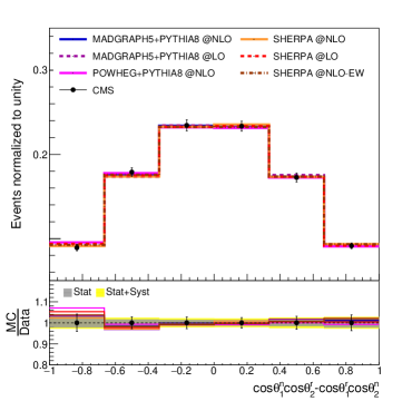
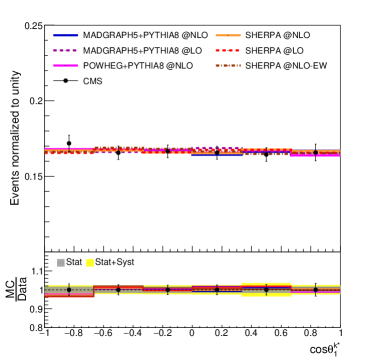
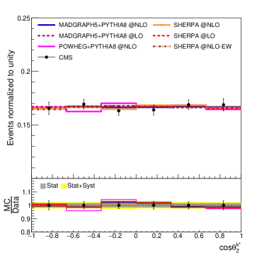
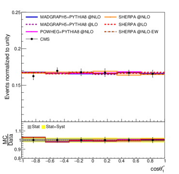
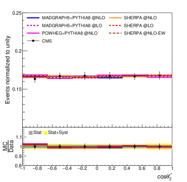
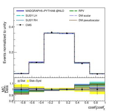
In figure 3, the diagonal spin correlation observables defined in eq. 11 are presented. There are no significant deviations in different MC approaches and different QCD corrections as well as EW correction. The experimental uncertainty comprise almost all variations of predictions.
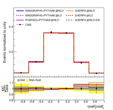
The predictions for the differential distributions of the observables , eq. 12, are considered in figure 4. Non-zero coefficients and are expected from mixed QCD-weak corrections correspond to ref. 0h . Due to smallness of this effect, scale, PDF and experimental uncertainties dominate it. Within the uncertainties, the experimental data and predictions for cross spin correlation observables are matched.
The normalized differential distributions in , eq. (9, 10), which is the indicator of the polarization of top quark and anti-quark are shown in figure 5. The polarization coefficients for all predictions behave similar in all distributions. CMS data and MC predictions are compatible within uncertainties. In the same way, the normalized differential distributions of predicted by MC, figure 6, are in agreement with data.
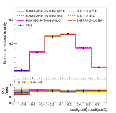


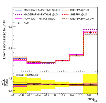
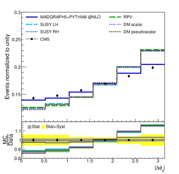
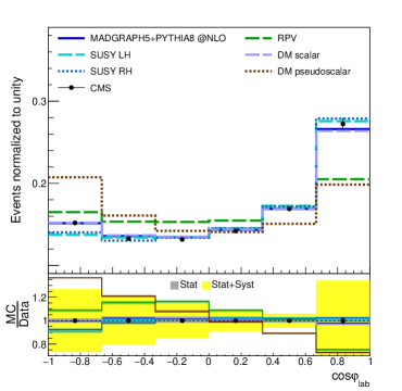
The differential distributions in the observables, which are calculated with kinematic variables of leptons in laboratory-frame, are in figure 7. When is considered with total uncertainty which is around , the shapes predicted by MadGraph5 and Sherpa ME generators are roughly consistent. Sherpa and MadGraph5 at LO accuracy show better performance than the samples simulated at NLO, this may be the result of real contributions at NLO accuracy spoiling the back-to-back alignment of the top quarks. Powheg is separated from the other MC predictions and the data about at low and high regions. For the distributions of , all MC predictions and the data are in good agreement in whole range, although the systematic uncertainties coming from PDF sets and scales are more than in almost whole regions. The huge systematic uncertainty as seen in the lower panel of the right plot in figure 7 is coming from PDF variations in Sherpa samples.
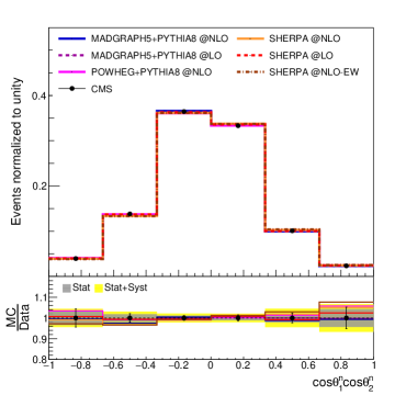
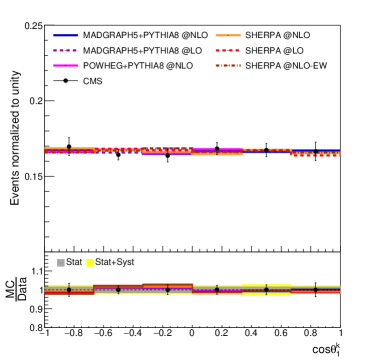
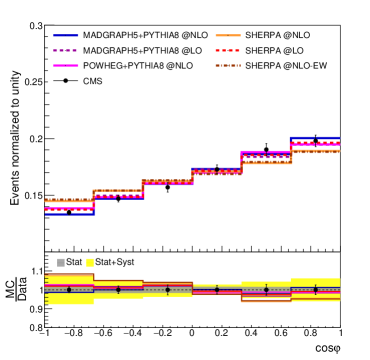
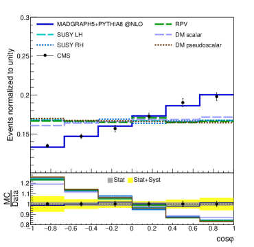
In distribution, figure 8, the predictions of MC generators are more similar compared to laboratory-frame distributions. While the distributions of different MC variations have considerably the same shape, Sherpa with NLO QCD accuracy and EW correction deviate from the others, especially at low , but are still in total uncertainty.
In second part of the analysis, we have investigated various new physics models with the help of the elements of spin density matrix. For top quark pair channel, most searches for SUSY and DM particles comprise generally high missing transverse energy region stem from undetected LSP and DM 1a ; 1b ; 0e ; 1d . The main point for the BSM analysis in this study is the models with low but also the same models with high , which are not excluded by CMS and ATLAS Collaborations yet, will be mentioned for the sake of broad phase space.

As mentioned earlier, we take into account three different BSM signal topologies to compare with SM predicted results and the data. The details of the event samples of the signals can be seen in section 1. The SUSY samples were simulated as unpolarized. To check importance of it, the R-Parity conserved SUSY sample is determined as two separate configurations having polarized stop quarks. To polarize the as fully left- (SUSY LH) and right-handed (SUSY RH), the distributions in the SUSY sample is multiplied by a weight obtained from the reweighting algorithm detailed in af . The second signal is that DM model having scalar or pseudoscalar mediator associated with top quark pair. Within this model, the collision process has missing transverse energy as in the model above. For both sample, the study is focused on a narrow phase space in which mass difference between and is slightly bigger than top or the mediator mass is relatively small, in this case 10 GeV. To ensure the larger phase space in the mass, the R-Parity violating (RPV) SUSY is included in the analysis framework. The mechanism of the R-Parity violation gives us three quarks decayed from . Thus in the pair production consists of only neutrinos from top quark decay chain. The following results for RPV SUSY are performed with a signal point of GeV. Furthermore, masses from GeV to GeV for RPV SUSY were analyzed and all mass points appear similarly.

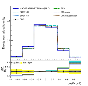
The distributions of spin correlation and polarization observables are presented in figures 9-14. The figures involve related BSM signals, CMS data and the nominal sample with systematic and statistical uncertainties calculated in the previous section. In the lower panels, the statistical uncertainties of the signals are specified on each signal sample.
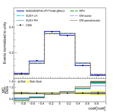
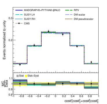
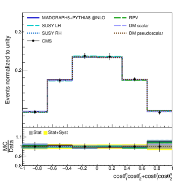
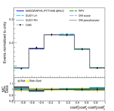
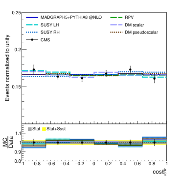
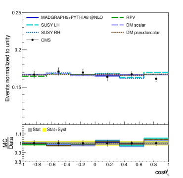
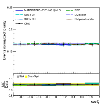
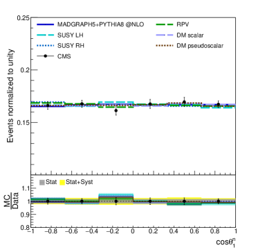
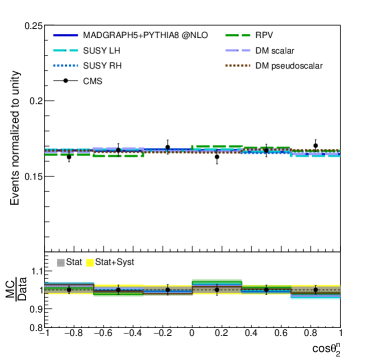
The differential distributions of the diagonal spin correlation observables in BSM signals are shown in figure 9. Almost all signals for and observables deviate up to from SM nominal predictions and the CMS data. For , the difference between signals and the nominal sample can be seen despite the domination of the uncertainties. It is seen that the scalar-mediated DM signal apart from the others has a non-zero diagonal spin correlation coefficient.
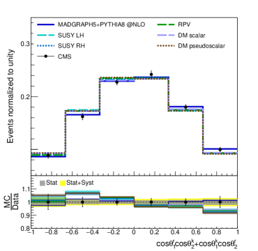
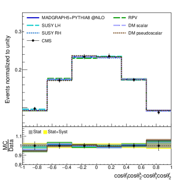
In figure 10, the distributions of the observables defined in equation 12 are discussed for signals with the nominal sample and the CMS data. The distribution in the upper left corner has a difference between signals and nominal sample because the coefficient of this observable is generated by P and CP conserving interactions as in the diagonal spin coefficients. For the other cross spin correlation observables, the distributions of signals and the nominal sample are compatible with the experimental data when considered total uncertainty.
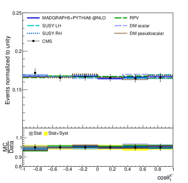
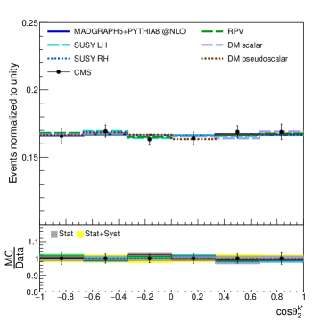
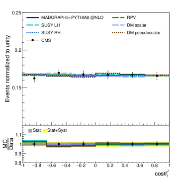
The observables in equations (9, 10) are not sensitive to small amount of top quark polarization predicted in both BSM and SM as seen in figures 11-12. The distributions are very flat for all predictions and the data. Furthermore, polarized stops do not have any effect on the distributions as shown in fully left and right-handed separated SUSY samples.
The laboratory frame observables are indicator of presence of spin correlations as in P- and CP-even observables. Especially the distribution in figure 13 reveals this with the difference between BSM and SM. Moreover, it can be seen that the dark matter model with scalar mediator has spin correlation though not as much as SM. In the with high systematic uncertainties, some BSM models act as in the SM while others deviate much more.
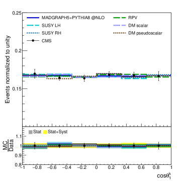
The last spin correlation sensitive observable is that the inner product of flight direction of two leptons in its own top quark center of mass frame (). In the figure 14, the sensitivity to spin correlation is seen in the DM with scalar mediator while not in the other BSM samples.
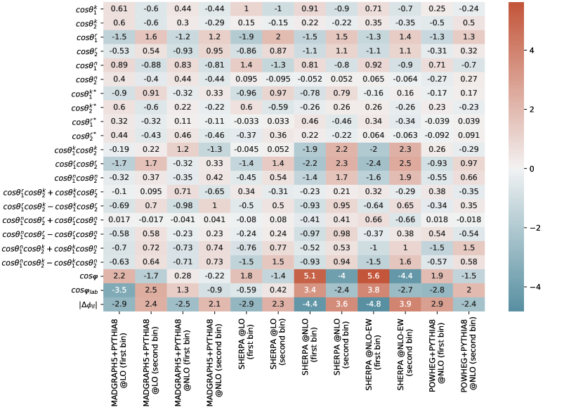
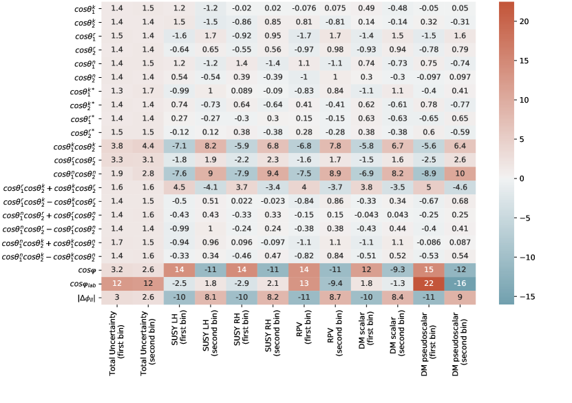
To get a general picture, all distributions of various MC event generator configurations, BSM signals and the CMS data for all observables presented in figures 3-14 are summarized as heat maps in figures 15-16. In these figures, each normalized distribution of each configuration is used as reduced bins from to to observe the degree of deviation of the distributions. Values on each cell in figures 15-16 indicate the percentage difference between rebinned normalized distributions of predictions or BSM signals and of the data. In figure 15, it can be explicitly seen that all MC event generator configurations explain the data, within total uncertainty, for distributions of the observables extracted from the spin density matrix. However, and laboratory-frame observables ( and ) show deviations of up to in NLO QCD accuracy in Sherpa, as well as the inclusion of EW correction. The positive or negative deviation (in percentage) of rebinned normalized distributions of the BSM signals from the data is shown in figure 16. The first two columns indicate, for each bin, absolute total uncertainty (statistical and systematic sum) calculated in each of the above distributions. This table is a beneficial tool to see the degree of deviation of the BSM signals from the experimental data in a particular region of each observable. With this sense, it is clearly seen that the , and observables as elements of the spin density matrix are sensitive to the considered BSM signals. In addition, all BSM signals for and seem to differ significantly from the experiment. Finally, it appears that the left or right-handed polarization of the stop quarks does not cause any notable change for these observables, whereas the DM signal with the scalar mediator has more spin correlation between the top quarks compared to the pseudoscalar mediator.
5 Conclusions and Outlook
In this work, we have made for the first time a comprehensive analysis of the spin correlation and polarization observable set and the direct angle-related observables between leptons in the production with dileptonic final states at TeV. This has provided us to investigate top quark pairs advanced properties for proton-proton collisions by using various MC event generator methods at LO, NLO QCD accuracy and NLO QCD with EW corrections in detail. For the distributions of the set of observables at the full phase space, we have compared our results with the unfolded data performed by CMS collaboration. Our study is mainly composed of two parts: the first is to compare different MC configurations with the experimental data and determine their effects on each variable, and the second is to find the degree of deviation of and DM signals from the data for each spin correlation observable. For a clear view of deviations from the data, we have created two heat map tables of SM and BSM samples with the set of observables, in figures 15-16.
Considering the different theoretical approaches, the polarization observables (including terms with modified axes) and the cross terms of the spin correlation observables are in agreement within the systematic and statistical uncertainty (around the ). Especially samples of Sherpa at NLO accuracy (and with electroweak corrections) for diagonal terms in the spin correlation observables tend to have more deviation (from to ) compared to the others (almost all under ) but they are still in total uncertainty. The biggest contribution to the uncertainty comes from the PDF variations of predictions at LO accuracy. Separation might be seen better in NLO calculations due to the less dependency of higher order calculations to the PDF variations. Furthermore, to be more accurate in predictions, it is needed to increase the statistics in experimental data, and upcoming LHC runs could provide this. The behavior of the different configurations can be clearly seen in the and distributions, the observables most sensitive to spin correlation in the top quark pair. The deviations up to in Sherpa samples (NLO and NLO-EW) for these observables, in figure 15, could be arisen from its approximation in hard and large angle emissions.
Figure 16 provides a complete map of the BSM signals according to the experiment, in the phase space of the related observables. Polarization and cross spin correlation observables (except ) are compatible for the BSM signals and the data, while the signals have good separation for P- and CP-even observables (up to ). Only the DM sample with a scalar mediator has spin correlation, unlike other BSM signals, but the spin correlation power in its top-quark pair is not as much as in the SM. Furthermore, polarized stop quarks of different composition have no impact observed on top quark spin correlation.
The different MC event generator configurations are compatible with each other, within total uncertainty, for the observables of spin correlation and polarization in the top quark pair. However, for some observables as mentioned above, there are small separations dominated by systematic uncertainties. Next-to-next-to leading order (NNLO) calculations can make these differences more visible by reducing systematic uncertainties, or they can reduce the difference between configurations by making more accurate calculations with higher-order ME calculations. Thereby, this gets NNLO calculations for theoretical predictions more important. Additionally, the observables may be used, especially in low missing transverse energy region, for searching BSM signals due to their sensitivity of contributions from parity and/or CP conserving or violating interactions.
Acknowledgements.
We thank Alexander Josef Grohsjean for discussions on spin correlation analysis, and Gurpreet Singh Chahal for contributions about Sherpa productions. This work is supported by Istanbul Technical University Research Fund under grant number TGA-2020-42345 and TUBITAK grant 121F065.References
- (1) W. Bernreuther, A. Brandenburg, Z. G. Si and P. Uwer, Spin properties of top quark pairs produced at hadron colliders, arXiv:hep-ph/0304244 [hep-ph].
- (2) W. Bernreuther and Z. G. Si, Distributions and correlations for top quark pair production and decay at the Tevatron and LHC, arXiv:1003.3926 [hep-ph].
- (3) W. Bernreuther, A. Brandenburg, Z.G. Si and P. Uwer, Top quark spin correlations at hadron colliders: Predictions at next-to-leading order QCD, Phys. Rev. Lett. 87, 242002 (2001), arXiv:hep-ph/0107086 [hep-ph].
- (4) A. Behring, M. Czakon, A. Mitov, A. S. Papanastasiou and R. Poncelet, Higher order corrections to spin correlations in top quark pair production at the LHC, arXiv:1901.05407 [hep-ph].
- (5) ATLAS Collaboration, Measurements of top-quark pair spin correlations in the channel at TeV using collisions in the ATLAS detector, Eur. Phys. J. C 80 (2020) 754, arXiv:1903.07570 [hep-ex].
- (6) M. Czakon, A. Mitov and R. Poncelet, NNLO QCD corrections to leptonic observables in top-quark pair production and decay, arXiv:2008.11133 [hep-ph].
- (7) CMS Collaboration, Probing the spin correlations of production at NLO QCD+EW, arXiv:2105.11478 [hep-ph].
- (8) W. Bernreuther, D. Heisler, and Z. G. Si, A set of top quark spin correlation and polarization observables for the LHC: Standard model predictions and new physics contributions, JHEP 12, 026 (2015), arXiv:1508.05271 [hep-ph].
- (9) CMS Collaboration, Measurement of the top quark polarization and spin correlations using dilepton final states in proton-proton collisions at TeV, Phys. Rev. D 100, 072002 (2019), arXiv:1907.03729 [hep-ex].
- (10) HSF Physics Event Generator WG, Challenges in Monte Carlo event generator software for High-Luminosity LHC, arXiv:2004.13687 [hep-ph].
- (11) T. Sjöstrand, Status and developments of event generators, PoS LHCP2016, 007 (2016), arXiv:1608.06425 [hep-ph].
- (12) LHC Higgs Cross Section Working Group, Handbook of LHC Higgs Cross Sections: 4. Deciphering the Nature of the Higgs Sector, CERN (2016), arXiv:1610.07922 [hep-ph].
- (13) CMS Collaboration, Measurement of jet substructure observables in events from proton-proton collisions at TeV, Phys. Rev. D 98, 092014 (2018), arXiv:1808.07340 [hep-ex].
- (14) S. Frixione, E. Laenen, P. Motylinski and B. R. Webber, Angular correlations of lepton pairs from vector boson and top quark decays in Monte Carlo simulations, JHEP 04, 081 (2007), arXiv:hep-ph/0702198 [hep-ph].
- (15) P. Z. Skands, B. R. Webber and J. Winter, QCD Coherence and the Top Quark Asymmetry, JHEP 07, 151 (2012), arXiv:1205.1466 [hep-ph].
- (16) CMS Collaboration, Combined searches for the production of supersymmetric top quark partners in proton-proton collisions at TeV, arXiv:2107.10892 [hep-ex].
- (17) ATLAS Collaboration, Search for direct top squark pair production in final states with two leptons in TeV collisions with the ATLAS detector, Eur. Phys. J. C77 (2017) 898, arXiv:1708.03247 [hep-ex].
- (18) ATLAS Collaboration, Search for new phenomena in events with two opposite-charge leptons, jets and missing transverse momentum in collisions at TeV with the ATLAS detector, JHEP 04 (2021) 165, arXiv:2102.01444 [hep-ex].
- (19) G. R. Farrar and P. Fayet, Phenomenology of the Production, Decay, and Detection of New Hadronic States Associated with Supersymmetry, Phys. Lett. B 76, 575-579 (1978).
- (20) R. Barbier et al., R-parity violating supersymmetry, Phys.Rept.420:1-202,(2005), arXiv:hep-ph/0406039 [hep-ph].
- (21) CMS Collaboration, Search for top squarks in final states with two top quarks and several light-flavor jets in proton-proton collisions at TeV, arXiv:2102.06976 [hep-ex].
- (22) J. Alwall, R. Frederix, S. Frixione, V. Hirschi, F. Maltoni, O. Mattelaer, H. S. Shao, T. Stelzer, P. Torrielli and M. Zaro, The automated computation of tree-level and next-to-leading order differential cross sections, and their matching to parton shower simulations, JHEP 07, 079 (2014), arXiv:1405.0301 [hep-ph].
- (23) T. Sjöstrand, S. Ask, J. R. Christiansen, R. Corke, N. Desai, P. Ilten, S. Mrenna, S. Prestel, C. O. Rasmussen and P. Z. Skands, An Introduction to PYTHIA 8.2, Comput. Phys. Commun. 191 (2015) 159, arXiv:1410.3012 [hep-ph].
- (24) S. Hoche, F. Krauss, N. Lavesson, L. Lonnblad, M. Mangano, A. Schalicke and S. Schumann, Matching Parton Showers and Matrix Elements, arXiv:hep-ph/0602031 [hep-ph].
- (25) R. Frederix and S. Frixione, Merging meets matching in MC@NLO, JHEP 12 (2012) 061, arXiv:1209.6215 [hep-ph].
- (26) T. Gleisberg et al, Event generation with SHERPA 1.1, JHEP 0902 (2009) 007, arXiv:0811.4622 [hep-ph].
- (27) F. Krauss, R. Kuhn and G. Soff, AMEGIC++ 1.0, A Matrix Element Generator In C++, JHEP 02 (2002) 044, arXiv:hep-ph/0109036 [hep-ph].
- (28) T. Gleisberg and S. Höche, Comix, a new matrix element generator, JHEP 12 (2008) 039, arXiv:0808.3674 [hep-ph].
- (29) F. Buccioni et al., OpenLoops 2, Eur. Phys. J. C 79 (2019) 866, arXiv:1907.13071 [hep-ph].
- (30) F. Cascioli, P. Maierhöfer and S. Pozzorini, Scattering Amplitudes with Open Loops, Phys. Rev. Lett. 108 (2012) 111601, arXiv:1111.5206 [hep-ph].
- (31) A. Denner, S. Dittmaier and L. Hofer, Collier: A fortran-based complex one-loop library in extended regularizations, Comput. Phys. Commun. 212 (2017) 220, arXiv:1604.06792 [hep-ph].
- (32) S. Schumann and F. Krauss, A Parton shower algorithm based on Catani–Seymour dipole factorisation, JHEP 0803 (2008) 038, arXiv:0709.1027 [hep-ph].
- (33) S. Höche, S. Schumann, and F. Siegert, Hard photon production and matrix-element parton-shower merging, PHYS.REV. D81 (2010) 034026, arXiv:0912.3501 [hep-ph].
- (34) S. Höche, F. Krauss, M. Schönherr and F. Siegert, QCD matrix elements + parton showers: The NLO case, JHEP 1304 (2013) 027, arXiv:1207.5030 [hep-ph].
- (35) S. Frixione and B. R. Webber, Matching NLO QCD Computations and Parton Shower Simulations, JHEP 0206 (2002) 029, arXiv:hep-ph/0204244 [hep-ph].
- (36) S. Frixione, P. Nason, and G. Ridolfi, A positive-weight next-to-leading-order Monte Carlo for heavy flavour hadroproduction, JHEP 09 (2007) 126, arXiv:0707.3088 [hep-ph].
- (37) P. Nason, A new method for combining NLO QCD with shower Monte Carlo algorithms, JHEP 11 (2004) 040, arXiv:hep-ph/0409146 [hep-ph].
- (38) S. Frixione, P. Nason, and C. Oleari, Matching NLO QCD computations with parton shower simulations: The POWHEG method, JHEP 11 (2007) 070, arXiv:0709.2092 [hep-ph].
- (39) S. Alioli, P. Nason, C. Oleari, and E. Re, A general framework for implementing NLO calculations in shower Monte Carlo programs: The POWHEG BOX, JHEP 06 (2010) 043, arXiv:1002.2581 [hep-ph].
- (40) NNPDF Collaboration, R.D. Ball et al., Parton distributions for the LHC Run II, JHEP 1504 (2015) 040, arXiv:1410.8849 [hep-ph].
- (41) NNPDF Collaboration, R.D. Ball et al., Parton distributions from high-precision collider data , Eur. Phys. J. C 77, no.10, 663 (2017), arXiv:1706.00428 [hep-ph].
- (42) A. Buckley, J. Ferrando, S. Lloyd, K. Nordström, B. Page, M. Rüfenacht, M. Schönherr and G. Watt, LHAPDF6: parton density access in the LHC precision era, Eur. Phys. J. C 75, 132 (2015), arXiv:1412.7420 [hep-ph].
- (43) H. L. Lai, M. Guzzi, J. Huston, Z. Li, P. M. Nadolsky, J. Pumplin, and C. P. Yuan, New parton distributions for collider physics, Phys. Rev. D 82, 074024 (2010), arXiv:1007.2241 [hep-ph].
- (44) L. A. Harland-Lang, A. D. Martin, P. Motylinski and R. S. Thorne, Parton distributions in the LHC era: MMHT 2014 PDFs, Eur. Phys. J. C 75, no. 5, 204 (2015), arXiv:1412.3989 [hep-ph].
- (45) ATLAS Collaboration, Studies on top-quark Monte Carlo modelling with Sherpa and MG5_aMC@NLO, ATL-PHYS-PUB-2017-007.
- (46) W. Bernreuther and A. Brandenburg, Tracing CP violation in the production of top quark pairs by multiple TeV proton-proton collisions, Phys. Rev. D 49, 4481 (1994), arXiv:hep-ph/9312210 [hep-ph].
- (47) W. Bernreuther and A. Brandenburg, Z. G. Si, and P. Uwer, Top quark pair production and decay at hadron colliders, Nucl. Phys. B690, 81 (2004), arXiv:hep-ph/0403035 [hep-ph].
- (48) K. Melnikov and M. Schulze, NLO QCD corrections to top quark pair production and decay at hadron colliders, JHEP 08, 049 (2009), arXiv:0907.3090 [hep-ph].
- (49) J. A. Aguilar-Saavedra, J. Carvalho, N. Castro, A. Onofre and F. Veloso, Probing anomalous Wtb couplings in top pair decays, Eur. Phys. J. C 50, 519 (2007), arXiv:hep-ph/0605190 [hep-ph].
- (50) J. Alcaraz and B. de la Cruz, Stopreweight, https://github.com/CMS-SUS-XPAG/Stopreweight, 2013.