Doing More with Less: Overcoming Data Scarcity for POI Recommendation via Cross-Region Transfer

Abstract.

Variability in social app usage across regions results in a high skew of the quantity and the quality of check-in data collected, which in turn is a challenge for effective location recommender systems. In this paper, we present Axolotl (Automated cross Location-network Transfer Learning), a novel method aimed at transferring location preference models learned in a data-rich region to significantly boost the quality of recommendations in a data-scarce region. Axolotl predominantly deploys two channels for information transfer, (1) a meta-learning based procedure learned using location recommendation as well as social predictions, and (2) a lightweight unsupervised cluster-based transfer across users and locations with similar preferences. Both of these work together synergistically to achieve improved accuracy of recommendations in data-scarce regions without any prerequisite of overlapping users and with minimal fine-tuning. We build Axolotl on top of a twin graph-attention neural network model used for capturing the user- and location-conditioned influences in a user-mobility graph for each region. We conduct extensive experiments on 12 user mobility datasets across the U.S., Japan, and Germany, using 3 as source regions and 9 of them (that have much sparsely recorded mobility data) as target regions. Empirically, we show that Axolotl achieves up to 18% better recommendation performance than the existing state-of-the-art methods across all metrics.

1. Introduction

As POI (Points-of-Interest) gathering services such as Foursquare, Yelp, and Google Places are becoming widespread, there is significant research in extracting location preferences of users to predict their mobility behavior and recommend next POIs that users are likely to visit (Manotumruksa et al., 2018; Likhyani et al., 2017; Cheng et al., 2013; Feng et al., 2018; Pan et al., 2019; Li et al., 2019). However, the quality of POI recommendations for users in regions where there is a severe scarcity of mobility data is much poorer in comparison with those from data-rich regions. This is a critical problem affecting the state-of-the-art approaches (Wang et al., 2019a; Yao et al., 2019a; He et al., 2020). The situation is further exacerbated in the recent times due to the advent of various restrictions for collecting personal data and growing awareness (in some geopolitical regions) about the need for personal privacy (Barkhuus and Dey, 2003; Wei et al., 2016). It not only means that there is overall reduction in the high quality (useful) data, but, even more importantly, it introduces a high-skew in the mobility data across different regions (see Figure 1) – primarily due to varying views towards personal privacy across these regions.
Therefore, current state-of-the-art methods struggle in low-data regions and the approaches that attempt to incorporate data from external sources suffer from the following limitations:

• limited to cold-start users from within a city (Ouyang et al., 2018; Wu et al., 2017; Li et al., 2020),

• focused only on using traffic network ignoring the use of social network of users and location dynamics (Wang et al., 2019a; Yao et al., 2019a; Pan et al., 2019),

• generate trajectories using a model learned on traffic-network images of source region (He et al., 2020; Fan et al., 2016), thus vulnerable to recaliberation,

• operating only for users who are common across locations (Dong et al., 2020; Li and Tuzhilin, 2020), or

• adopting a limited level of transfer through domain-invariant features (Krishnan et al., 2020) –like the spending capacity or the users’ age, thus constrained by the feature unavailability in public datasets.

Unfortunately, none of these approaches, especially those based on visual-data (i.e., traffic and location images), can be easily re-calibrated for a target POI network due to the varied spatial density, location category and lack of user-specific features in public POI datasets.

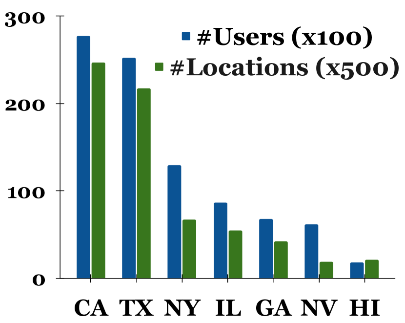
(a) State-wise Data

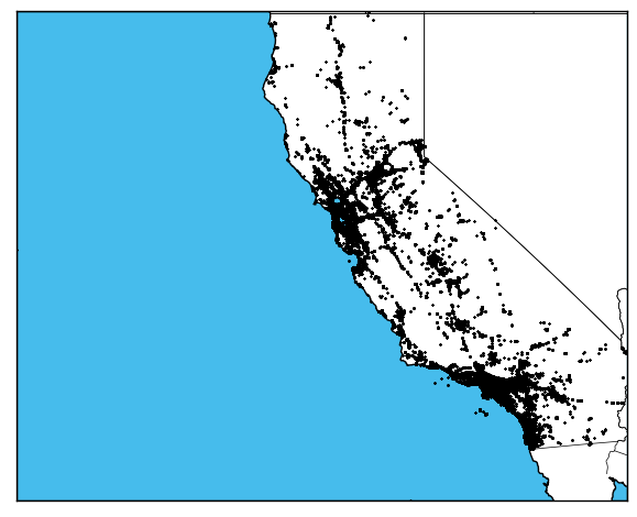
(b) California

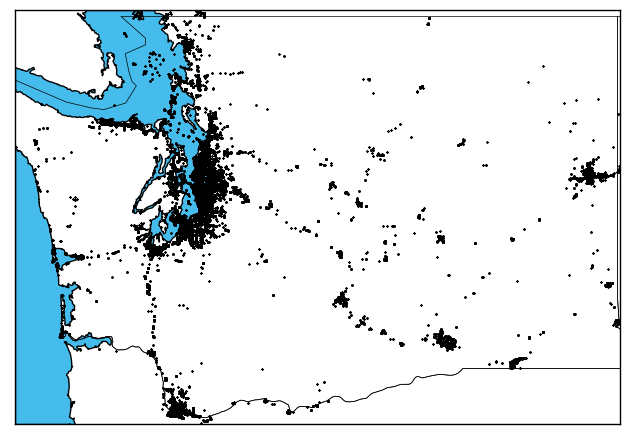
(c) Washington

Figure 1. Skew in the volume of mobility data across different states in the US (Figure 1(a)) and the large variation in region-specific density of mobility data between California and Washington in Figures  1(b) and  1(c) respectively (based on Gowalla dataset (Scellato et al., 2011)).

1.1. Contributions

In this paper, we present Axolotl(Automated cross Location-network Transfer Learning), a novel meta learning-based approach for POI recommendation in limited-data regions while transferring model parameters learned at a data-rich region without any prerequisite of inter-region user overlap. Specifically, we use a hierarchical multi-channel learning procedure with a novel meta-learning (Finn et al., 2017; Lee et al., 2019a) extension for geographical scenarios called spatio-social meta-learning (SSML), that learns the model parameters by jointly minimizing the region-specific social as well as location recommendation losses, and a cross-region transfer via clusters (Yao et al., 2019a; Wang et al., 2019a) of user and locations with similar preferences by minimizing an alignment loss (Jang et al., 2019; Zagoruyko and Komodakis, 2017), to achieve high performance even in extremely limited-data regions. We represent the POI network of each region via a heterogeneous graph with users and locations as nodes and capture the user-location inter-dependence and their neighborhood structure via a twin graph attention model (Wu et al., 2019b; Zhuang and Ma, 2018). The graph-attention model aggregates all four aspects of user and location influences (Fan et al., 2019; Wu et al., 2016) namely, (i) users’ social neighborhood and their location affinity to construct user-specific and location-conditioned representations, and (ii) similarly for each location, its neighboring locations and associated user affinity to obtain a locality-specific and user-conditioned representations. We combine this multi-faceted information to determine the final user and location representations which are used for POI recommendation. We highlight the region-size invariant performance of Axolotl by using regions with different spatial granularities, i.e. large and small states for Germany and U.S respectively, and prefectures for Japan.

In summary, the key contributions we make in this paper via Axolotl are three-fold:

1. Region-wise Transfer: We address the problems associated with POI recommendation in limited data regions and propose Axolotl, a cross-region model transfer approach for POI recommendation that does not require common users and their traces across regions. It utilizes a novel spatio-social meta-learning based transfer and minimizes the divergence between user-location clusters with similar characteristics.

2. User-Location Influences: Our twin graph attention-based model combines user and location influences in heterogeneous mobility graphs. This is the first approach to combine these aspects for addressing the data scarcity problem with POI recommendation. Axolotl is robust to network size, trajectory spread, and check-in category variance making it more suitable for transfer across geographically distant regions (and even across different networks).

3. Detailed Empirical Evaluation: We conduct thorough experiments over 12 real-world points-of-interest datasets from the U.S, Japan, and Germany, at different region-wise granularity. They highlight the superior recommendation performance of Axolotl over state-of-the-art methods across all metrics.

2. Related Work

In this section, we introduce key related work for this paper. It mainly falls into following categories: 1) Mobility Prediction; 2) Graph based recommendations; 3) Transfer Learning and Mobility.

Mobility Prediction: Understanding the mobility dynamics of a user is widely studied using different data sources (Zheng, 2011; Cho et al., 2011). Early efforts relied on taxi datasets to study individual trajectories (Li et al., 2018b; Guo et al., 2019). However, these approaches are limited by the underlying datasets as it excludes two critical aspects of a mobility network; the social friendships and location categories. The social network is used to model the influence dynamics across different users (Likhyani et al., 2017; Manotumruksa et al., 2018) and the POI categories capture the different preferences of an individual (Likhyani et al., 2020; Cheng et al., 2013). We utilize user POI social networks for our model as these datasets provide both: a series of social dynamics for different users and location-specific interest patterns for a user. These are essential for tasks such as location-specific advertisements and personalized recommendations. Standard POI models that utilize an RNN (Chakraborty et al., 2020; Manotumruksa et al., 2018; Zheng, 2011; Liu et al., 2016; Feng et al., 2018) or a temporal point process (Gupta et al., 2021; Likhyani et al., 2020; Gupta and Bedathur, 2021) are prone to irregularities in the trajectories. These irregularities arise due to uneven data distributions, missing check-ins, and social links. Moreover, these approaches consider the check-in trajectory for each user as a sequence of events and thus have limited power to capture the user-location inter-dependence through their spatial neighborhood, i.e. the location-sensitive information that influences all neighborhood events. Recent approaches (Wang et al., 2019a; Yao et al., 2019a), harness the spatial characteristics by generating an image corresponding to each user trajectory and then utilize a CNN as an underlying model. Such approaches based on visual data, and all CNN-based approaches, are limited by the image characteristics such as resolution and interpolation. Modern POI recommendation approaches such as (Yang et al., 2019) model the spatial network as a graph and utilize a random-walk-based model, with (Wu et al., 2019a) proposing a graph-based neural network based model to incorporate structural information of the network. Unfortunately, none of these approaches are designed for mobility prediction in limited data regions.

Graph based Recommendation: Existing graph embedding approaches focus on incorporating the node neighborhood proximity in a classical graph in their embedding learning process (Grover and Leskovec, 2016; Yang et al., 2019). For example  (He et al., 2017a) adopts a label propagation mechanism to capture the inter-node influence and hence the collaborative filtering effect. Later, it determines the most probable purchases for a user via her interacted items based on the structural similarity between the historical purchases and the new target item. However, these approaches perform inferior to model-based CF methods, since they do not optimize a recommendation-specific loss function. The recently proposed graph convolutional networks (GCNs) (Kipf and Welling, 2017) have shown significant prowess for recommendation tasks in user-item graphs. The attention-based variant of GCNs, graph attention networks (GATs) (Veličković et al., 2018) are used for recommender systems in information networks (Fan et al., 2019; Wang et al., 2019b), traffic networks (Guo et al., 2019; Li et al., 2018b) and social networks (Ying et al., 2018a; Zhang et al., 2019). Furthermore, the heterogeneous nature of these information networks comprises of multi-faceted influences that led to approaches with dual-GCNs across both user and item domains (Zhuang and Ma, 2018; Fan et al., 2019). However with POI networks, the disparate weights, location-category as node feature, and varied sizes, these models cannot be generalized for spatial graphs.

Clustering in Spatial Datasets: In addition to the twin-GAT model, Axolotl includes an alignment loss for cross-region transfer via clusters of users and locations with similar preferences. Due to the disparate features in our spatial graph, identifying the optimal number of clusters for the source and target region is a non-trivial task. Thus, we highlight a few key related works for clustering POIs and users in a spatial graph. Standard community-detection algorithms for spatial datasets (Likhyani et al., 2020; Noulas et al., 2011; Wang et al., 2012; Li et al., 2018a) are not suitable for grouping POIs as they ignore the graph structure, POI-specific features such as categories, geographical distances, and the order of check-ins in a user trajectory. Moreover, the clustering performance of these methods is highly susceptible to the hyper-parameter values used in a setting. Recent approaches (Morris et al., 2019; Lee et al., 2019b; Ying et al., 2018b; Abu-El-Haija et al., 2019; Gao and Ji, 2019) can automatically identify the number of clusters in a graph by capturing higher-order semantics between graph nodes, however, their application to graphs in spatial and mobility domains have certain challenges. In detail, (i) DiffPool (Ying et al., 2018b) can learn differentiable clusters for POIs and users for each region, however, these assignments are soft i.e., without definite boundaries between distant POI clusters and, moreover, have a quadratic storage complexity; (ii) Gao and Ji (2019) ignores the topology of the underlying spatial graph; (iii) Lee et al. (2019b) can be extended to spatial graphs, however, has limited scalability due to its self-attention (Vaswani et al., 2017) based procedure; (iv) Morris et al. (2019) can incorporate higher-order structure in a POI graph using multi-dimensional Weisfeiler-Leman graph isomorphism; and (v) Abu-El-Haija et al. (2019) can learn inter-user and inter-POI relationships by mixing feature representations of neighbors at various distances. However, due to the presence of two types of graph nodes – user and POI – identifying higher-order relationships by solely considering POI or user nodes is challenging. In addition,  Chen et al. (2021) uses a differentiable grouping network to discover the latent dependencies in a spatial network but is limited to air-quality forecasting. We highlight that though these approaches can be plugged-in with Axolotl, they have an additional computation cost that gets further amplified due to the repetitive clustering procedure required in Axolotl (please refer to Section 4.3.2). However, we note that using these approaches over Axolotl while simultaneously maintaining the scalability is a probable future work of this paper.

Transfer Learning and Mobility: Transfer learning has long been addressed for tasks involving sparse data (Jang et al., 2019; Finn et al., 2017) with applications to recommender systems as well (Vartak et al., 2017; Lee et al., 2019a; Li and Tuzhilin, 2020). Transfer-based spatial applications deploy CNNs across regions and achieve significant improvements in limited data-settings (Wang et al., 2019a; Yao et al., 2019a). However, these approaches are restricted to non-structural data and a graph-based approach has not been explored by the previous literature. (Li et al., 2020) extends meta-learning to enhance recommendations in a POI setting, but is limited to a specific region. Information transfer across graphs is not a trivial task (Lee et al., 2017; Yao et al., 2020; Krishnan et al., 2020) and recent mobility models that incorporate graphs with meta-learning in (Pan et al., 2019; Manotumruksa et al., 2019) are either limited to traffic datasets and do not incorporate the social network or are limited to new trajectories (He et al., 2020; Fan et al., 2016). From our experiments, we prove that a mere fine-tuning on the target data is susceptible to large cross-data variances and thus re-calibrating a generative model is not a trivial task in mobility-based networks.

3. Problem Formulation

We consider POI data for two regions, a source and a target denoted by $\boldsymbol{\mathcal{D}}^{src}$ and $\boldsymbol{\mathcal{D}}^{tgt}$. We denote the users and locations in source and target networks as $\mathcal{U}^{src},\mathcal{P}^{src}\in\boldsymbol{\mathcal{D}}^{src}$ and $\mathcal{U}^{tgt},\mathcal{P}^{tgt}\in\boldsymbol{\mathcal{D}}^{tgt}$ correspondingly with no common entries $\mathcal{U}^{src}\cap\mathcal{U}^{tgt}=\mathcal{L}^{src}\cap\mathcal{L}^{tgt}=\varnothing$. In other words, we do not need a common user between two regions to perform a cross-region mobility knowledge transfer. With a slight abuse of notation, the network for any region –either target or source– is assumed to consist of users $|\mathcal{U}|=M$, locations $|\mathcal{P}|=N$ and an affinity matrix $\boldsymbol{R}=\{r_{ul}\}_{M\times N}$. We populate entries in $\boldsymbol{R}$ as row-normalized number of check-ins made by a user to a location (i.e., multiple check-ins mean higher value). This can be further weighed by the user-location ratings, if available. We denote a pair of users as $u_{i},u_{j}$ and locations as $l_{a},l_{b}$. We also assume that for each location $l_{a}$ we have one (or more) category label (such as Jazz Club, Cafe, etc.).

Problem Statement 0 (Target Region POI Recommendation).

Given the mobility data of source and target regions, $\boldsymbol{\mathcal{D}}^{src}$ and $\boldsymbol{\mathcal{D}}^{tgt}$, our aim is to transfer the rich dynamics in source region to improve POI recommendation for users in the target region. Specifically, maximize the following probability:

(1) $$P^{*}=\arg\max\{\mathbb{E}[r_{u_{i},l_{a}}^{tgt}|\boldsymbol{\mathcal{D}}^{src},\boldsymbol{\mathcal{D}}^{tgt}]\},$$

where $\mathbb{E}[r^{tgt}_{u,l}]$ calculates the expectation of location $l_{a}$ in the target region being visited by the user $u_{i}$, thus $r_{u_{i},l_{a}}^{tgt}\in\boldsymbol{R}^{tgt}$, given the mobility data of users from both source and target regions. Simultaneously for a region, our objective as personalized location recommendation is to retrieve, for each user, a ranked list of candidate locations that are most likely to be visited by her based upon the past check-ins available in the training set.

3.1. User-Location Graph Construction

For each region, we construct a heterogeneous user-location graph $\mathcal{G}^{src}$ and $\mathcal{G}^{tgt}$ but we describe generically as $\mathcal{G}=\{\mathcal{U}\cup\mathcal{P},\mathcal{E}\}$ with each user and location as a node. The disparate edges $\mathcal{E}_{u},\mathcal{E}_{l},\mathcal{E}_{r}\in\mathcal{E}$ determine the user-user, location-location and user-location relationships respectively. The structure of the graph is as follows:

• An edge, $e_{u_{i},u_{j}}\in\mathcal{E}_{u}$, between two users, $u_{i}$ and $u_{j}$ is denotes a social network friendship.

• We form an edge, $e_{l_{a},l_{b}}\in\mathcal{E}_{l}$, between two locations when any user has consecutive check-ins between them – i.e., a check in at $l_{a}$ (or $l_{b}$) followed immediately by $l_{b}$ (or $l_{a}$) with edge weight based on the geographical distance (Li et al., 2018b; Zhang et al., 2019) between the two locations. Specifically, we use non-linear decay with distance as:

  $$w(e_{l_{a},l_{b}})=\begin{cases}\exp\left(-\frac{d(l_{a},l_{b})}{\sigma^{2}}\right),&\mathrm{if~{}}d(l_{a},l_{b})\leq\kappa,\\ 0&\mathrm{otherwise},\end{cases}$$

  where $d(l_{a},l_{b})$ is the haversine (Contributors, 2021b) distance between the two locations.

• A check-in by user $u_{i}$ at location $l_{a}$ results in a user-location edge, $e_{u_{i},l_{a}}\in\mathcal{E}_{r}$.

We also use the following notations to define different neighborhoods that will be used in our model description later: (1) $\mathcal{N}_{u_{i}}=\left\{u_{k}:e_{u_{i},u_{k}}\in\mathcal{E}_{u}\right\}$: the social neighborhood of user $u_{i}$, (2) $\mathcal{N}_{l_{a}}=\left\{u_{k}:e_{u_{k},l_{a}}\in\mathcal{E}_{r}\right\}$: the user neighborhood of location $l_{a}$, (3) $\mathcal{S}_{u_{i}}=\left\{l_{k}:e_{u_{i},l_{k}}\in\mathcal{E}_{r}\right\}$: the location neighborhood of user $u_{i}$, and, finally, (4) $\mathcal{S}_{l_{a}}=\left\{l_{k}:e_{l_{a},l_{k}}\in\mathcal{E}_{l}\right\}$: locations in the spatial vicinity of $l_{a}$. Note that the graph $\mathcal{G}$ can also be enriched with all edges as weighted (Wu et al., 2019a) conditioned on the availability of different features. However, we present a general framework which can be easily extended to such settings.

Table 1. Summary of Notations Used.

Notation	Description
$\boldsymbol{\mathcal{D}}^{src},\boldsymbol{\mathcal{D}}^{tgt}$	Datasets for source and target regions
$\boldsymbol{R}$	Normalized user to location preference matrix
$\boldsymbol{U}_{l},\boldsymbol{U}_{s},\boldsymbol{U}_{f}$	User’s latent, location-based and final representations
$\boldsymbol{L}_{l},\boldsymbol{L}_{s},\boldsymbol{L}_{f}$	Location’s latent, user-based and final representations
$\Phi_{1\cdots 4}$	Graph Attention Networks in Axolotl
$\psi_{1\cdots 4}$	MLP layers to calculate attention weights for $\Phi_{1\cdots 4}$
$\varphi_{1\cdots 3}$	MLPs for final user and location embeddings, and affinity prediction
$\mathcal{L}_{p},\mathcal{L}_{s},\mathcal{L}_{c}$	Affinity, social prediction and Cluster-based loss
$K$	No. of clusters in source and target region
$N_{u}$	No. of target region based updates for SSML
$M_{t}$	Iterations before cluster-transfer
$\boldsymbol{U}^{tgt}_{c},\boldsymbol{L}^{tgt}_{c}$	User and location clusters for target region
$\boldsymbol{U}^{src}_{c},\boldsymbol{L}^{src}_{c}$	User and location clusters for source region

4. Axolotl Framework

In this section we first describe in detail the basic model of Axolotl along with its training procedure. Then we present the key feature of Axolotl, viz., its ability to transfer model parameters learned from data-rich region to data-scarce region. For a specific region, we embed all users in $\mathcal{U}$ and all locations in $\mathcal{P}$ through embedding matrices $\boldsymbol{U}=\{\boldsymbol{u}_{i}\}_{M\times D}$ and $\boldsymbol{L}=\{\boldsymbol{l}_{a}\}_{N\times D}$ respectively with $D$ as the embedding dimension. A summary of all notations is given in Table 1.

4.1. Basic Model

In the graph model of Axolotl, called Axo-basic, we capture the four aspects of influence propagation –namely, user-latent embeddings ($\boldsymbol{U}_{l}\in\mathbb{R}^{M\times D}$), location-conditioned user embeddings ($\boldsymbol{U}_{s}\in\mathbb{R}^{M\times D}$), location-latent embeddings ($\boldsymbol{L}_{l}\in\mathbb{R}^{N\times D}$), and user-conditioned location embeddings ($\boldsymbol{L}_{s}\in\mathbb{R}^{N\times D}$)– illustrated in Figure  2.

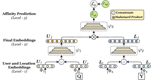
Figure 3. System architecture of Axo-basic that shows level-wise embedding computation and affinity prediction. User-Latent ($\boldsymbol{U}_{l}$) and Location conditioned ($\boldsymbol{U}_{s}$) embeddings are combined to form a final user embedding ($\boldsymbol{U}_{f}$) and similarly for location, $\boldsymbol{L}_{l}$ and $\boldsymbol{L}_{s}$ are combined to $\boldsymbol{L}_{f}$.

The basic model of Axolotl captures these four aspects using different graph attention networks, resulting in a twin-graph architecture as shown in Figure 3. In the rest of this section, we first describe each of the graph attention components and the prediction model in the basic model of Axolotl. Subsequently, we delineate the information transfer component that operates over this basic model.

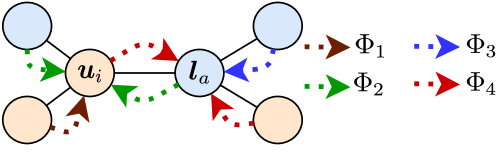
Figure 2. Different node and edge types in our graph model (users are in yellow and locations are in blue). The dashed arrows represent various influences and corresponding GATs ($\Phi_{i},i=1,2,3,4$) in Axolotl.

GAT for User Latent Embedding($\Phi_{1}$): In each iteration, using the available user embeddings, $\boldsymbol{U}$, we aggregate each user’s social neighborhood to obtain a new latent representation of the user. We denote this embedding as $\boldsymbol{U}_{l}$ and calculate as follows:

(2) $$\boldsymbol{u}_{l,i}=\sigma\bigg{(}\sum_{u_{k}\in\mathcal{N}_{u_{i}}}\boldsymbol{\alpha}^{\Phi_{1}}_{u_{i},u_{k}}\left(\mathbf{W}_{\Phi_{1}}\boldsymbol{u}_{k}+\mathbf{b}_{\Phi_{1}}\right)\bigg{)},\,\boldsymbol{u}_{l,i}\in\boldsymbol{U}_{l},$$

where $u_{i}\in\mathcal{U},\mathcal{N}_{u_{i}},\sigma,\mathbf{W}_{\Phi_{1}}$ and $\mathbf{b}_{\Phi_{1}}$ are the user node ${u}_{i}$, nodes in the social neighborhood of ${u}_{i}$, the activation function, the weight matrix and the bias vector respectively. $\boldsymbol{\alpha}^{\Phi_{1}}_{u_{i},u_{k}}$ determines the attention weights between user embeddings $\boldsymbol{u}_{k}$ and $\boldsymbol{u}_{i}$ given by:

(3) $$\boldsymbol{\alpha}^{\Phi_{1}}_{u_{i},u_{k}}=\frac{\exp\big{(}\psi_{1}(\boldsymbol{u}_{i},\boldsymbol{u}_{k})\big{)}}{\sum_{u_{j}\in\mathcal{N}_{u_{i}}}\exp\big{(}\psi_{1}(\boldsymbol{u}_{i},\boldsymbol{u}_{j})\big{)}},$$

where, $\psi_{1}(\boldsymbol{u}_{i},\boldsymbol{u}_{j})=\mathtt{LeakyReLU}(\mathbf{G}_{\Phi_{1}}\otimes(\boldsymbol{u}_{i}\mathbin{\|}\boldsymbol{u}_{j}))$ calculates the inter-user attention weights with learnable parameter $\mathbf{G}_{\Phi_{1}}$.

GAT for Location-conditioned User Embeddings ($\Phi_{2}$): To encapsulate the influence on a user based on the her check-ins as well as those by her social neighborhood, our embeddings must include location information for all check-ins made by different users in her social proximity. For this purpose, we first need to aggregate the location embeddings for every check-in made by a user ($u_{i}$) as her location-based embedding, $\boldsymbol{Q}=\{\boldsymbol{q}_{i}\}_{M\times D}$. We note that the category of a check-in location is arguably the root-cause for a user to visit the location and thus to capture the location-specific category and the user-category affinity in these embeddings, we populate $\boldsymbol{Q}$ using a max-pooling aggregator across each location embedding weighted by the probability of a category to be in a user’s check-in locations. That is,

(4) $$\boldsymbol{q}_{i}=\mathtt{MaxPool}\bigg{[}\sum_{l_{k}\in\mathcal{S}_{u_{i}}}\mathrm{p}^{u_{i}}_{(l_{k})}\cdot\boldsymbol{l}_{k}\bigg{]},\quad\forall\boldsymbol{q}_{i}\in\boldsymbol{Q},$$

where $\mathcal{S}_{u_{i}}$, $\mathrm{p}^{u_{i}}_{(l_{k})}$ respectively denote the location neighborhood of $u_{i}$ and the probability of a POI-category to be present in the past check-ins of $u_{i}$. We calculate $\mathrm{p}^{u_{i}}_{(l_{k})}$ as the fraction of check-ins made by the user to POIs of the specific category with the total number of her check-ins. Mathematically,

(5) $$\mathrm{p}^{u_{i}}_{(l_{k})}=\frac{\text{No. of check-ins by $u_{i}$ at POIs with category same as $l_{k}$}}{\text{Total no. of check-ins by $u_{i}$}},$$

We calculate these probabilities for every POI category and these values are user-specific. Moreover, the values of $\mathrm{p}^{u_{i}}_{(l_{k})}$ can be considered as the explicit category preferences of a user $u_{i}$.
Later, to get the influence of neighborhood locations on a user, we aggregate the location-based neighbor embeddings $\boldsymbol{Q}$ for each user (${u}_{i}$) based on her social network as:

(6) $$\boldsymbol{u}_{s,i}=\sigma\bigg{(}\sum_{u_{k}\in\mathcal{N}_{u_{i}}}\boldsymbol{\alpha}^{\Phi_{2}}_{u_{i},u_{k}}\left(\mathbf{W}_{\Phi_{2}}\boldsymbol{q}_{k}+\mathbf{b}_{\Phi_{2}}\right)\bigg{)},\,\boldsymbol{u}_{s,i}\in\boldsymbol{U}_{s},$$

where $\boldsymbol{\alpha}^{\Phi_{2}}_{u_{i},u_{k}}$ is the attention weight for quantifying the influence a user has on another through its check-ins and is formulated using $\psi_{2}$ similar to $\psi_{1}$ (Eqn  3). The resulting embedding $\boldsymbol{U}_{s}$ is the location-conditioned user embedding.

GAT for Location Latent Embedding ($\Phi_{3}$): Similar to $\Phi_{1}$, we aggregate the neighborhood of each location, $\boldsymbol{l}_{a}\in\boldsymbol{L}$, to get a latent representation of each location. To factor the inter-location edge-weight in our embeddings, we sample locations from the neighborhood with probability proportional to $w(e_{l_{a},l_{b}})$, i.e., closer the locations higher their repetitive sampling. These sampled locations represent the vicinity of the check-in and we encapsulate them to get the latent location representation.

(7) $$\boldsymbol{l}_{l,a}=\sigma\bigg{(}\sum_{l_{k}\in\mathcal{S}_{l_{a}}}\boldsymbol{\alpha}^{\Phi_{3}}_{l_{a},l_{k}}\left(\mathbf{W}_{\Phi_{3}}\boldsymbol{l}_{k}+\mathbf{b}_{\Phi_{3}}\right)\bigg{)},\,\forall l_{a}\in\mathcal{P},\boldsymbol{l}_{l,a}\in\boldsymbol{L}_{l},$$

where $\boldsymbol{\alpha}^{\Phi_{3}}_{l_{a},l_{k}}$ is again formulated as in Equation 3, using $\psi_{3}(\boldsymbol{l}_{a},\boldsymbol{l}_{k})$.

GAT for User-conditioned Location Embedding($\Phi_{4}$): Similar to $\Phi_{2}$, we need to capture the influence of different users with check-ins nearby to the current location $l_{a}$. Thus we use a max-pool aggregator to capture the user neighborhood of each location weighted by its affinity towards the location category. Through this, we aim to encapsulate the locality-specific user preferences, i.e. the counter-influence of $\boldsymbol{Q}$ in $\Phi_{2}$, denoted as $\boldsymbol{Y}=\{\boldsymbol{y}_{a}\}_{N\times D}$.

(8) $$\boldsymbol{y}_{a}=\mathtt{MaxPool}\bigg{[}\sum_{{u}_{k}\in\mathcal{N}_{l_{a}}}\mathrm{p}^{l_{a}}_{(u_{k})}\cdot\boldsymbol{u}_{k}\bigg{]},\quad\forall\boldsymbol{y}_{a}\in\boldsymbol{Y},$$

where, $\mathrm{p}^{l_{a}}_{(u_{k})}$ denotes the category affinity of all users in the neighborhood $\mathcal{N}_{l_{a}}$ of a location $l_{a}$. We calculate $\mathrm{p}^{l_{a}}_{(u_{k})}$ for each user as the fraction of check-ins of a user $u_{k}$ with the total check-ins for all users in $\mathcal{N}_{l_{a}}$ at the POIs with category same as $l_{a}$. Mathematically,

(9) $$\mathrm{p}^{l_{a}}_{(u_{k})}=\frac{\text{No. of check-ins by $u_{k}$ with category {`cat'}}}{\text{No. of check-ins by users in $\mathcal{N}_{l_{a}}$ with category {`cat'}}},$$

where ‘cat’ denotes the category of POI $l_{a}$. Moreover, these probabilities are specific to each POI and can be interpreted as the affinity of nearby users towards the POI category. Similar to $\Phi_{3}$, we aggregate the location neighborhood using an edge-weight based sampling on $\boldsymbol{Y}$ to get user-conditioned location embedding $\boldsymbol{L}_{s}$ with parameters $\mathbf{W}_{\Phi_{4}},\mathbf{b}_{\Phi_{4}}$ and $\boldsymbol{\alpha}^{\Phi_{4}}$ and $\psi_{4}(\boldsymbol{y}_{a},\boldsymbol{y}_{b})$.

4.2. Model Prediction

We combine the four representations of users and locations developed above using fully-connected layers, with a concatenated input of $\boldsymbol{U}_{l}$ and $\boldsymbol{U}_{s}$ for final user embedding $\boldsymbol{U}_{f}=\varphi_{1}\left(\boldsymbol{U}_{l}\mathbin{\|}\boldsymbol{U}_{s}\right)$; and similarly for locations $\boldsymbol{L}_{l}$ and $\boldsymbol{L}_{s}$ to obtain final location embedding $\boldsymbol{L}_{f}=\varphi_{2}\left(\boldsymbol{L}_{l}\mathbin{\|}\boldsymbol{L}_{s}\right)$. Finally, we estimate a user’s affinity to check-in at a location by a Hadamard (element-wise) product between the corresponding representations. Formally,

(10) $$\widehat{r_{ul}}=\varphi_{3}\left(\boldsymbol{U}_{f}\,\otimes\,\boldsymbol{L}_{f}\right),$$

where $\varphi_{1}(\cdot)$, $\varphi_{2}(\cdot)$ and $\varphi_{3}(\cdot)$ represent fully-connected neural layers.

The parameters are optimized using a mean-squared error that considers the difference between the user’s predicted and the actual affinity towards a location, with $L_{1}$ regularization over the trainable parameters.

(11) $$\mathcal{L}_{p}=\sum_{(\forall u,l)}\big{\lVert}\widehat{r_{ul}}-r_{ul}\big{\rVert}^{2}+\lambda_{p}\big{\lVert}\Theta_{pred}\big{\rVert}.$$

$\Theta_{pred}$ refers to all the trainable parameters in Axolotl for a region-specific prediction including the weights for all attention networks.

4.3. Axolotl: Information Transfer

We now turn our attention to the central theme of this paper, namely, the training procedure for Axolotl along with its cluster-wise transfer approach. We reiterate that we do not expect any common users/POIs between source and target regions, and thus the only feasible way to transfer mobility knowledge using the trained model parameters and the user-POI embeddings. Specifically, there are two channels of learning for Axolotl, (1) Spatio-Social Meta-learning based optimization, and (ii) Region-wise cluster alignment loss.

4.3.1. Spatio-Social Meta-Learning (SSML)

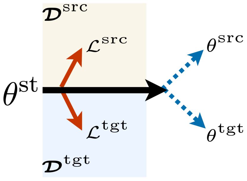
(a) MAML

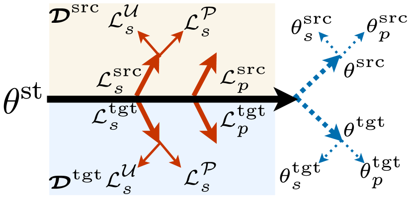
(b) SSML

Figure 4. The difference between MAML(fig 4(a)) and our SSML (fig 4(b)) is that the latter optimizes parameters in a hierarchy i.e. user and location parameters are updated for neighborhood prediction and then combined for POI recommendation. (Best viewed in color).

Meta-learning has long been proposed to alleviate data scarcity problem in spatial datasets (Pan et al., 2019; Yao et al., 2019a; Li et al., 2020). Specifically, in meta-learning, we aim to learn a joint parameter initialization for multiple tasks by simultaneously optimizing the prediction loss for each task. However, there is a high variance in data-quality between the regions $\boldsymbol{\mathcal{D}}^{src}$ and $\boldsymbol{\mathcal{D}}^{tgt}$ and thus a vanilla meta-learning —also called a model agnostic meta-learning (MAML) (Finn et al., 2017)— will not be sufficient as the target region is expected to have nodes with limited interactions. Such nodes, due to their low contribution in the loss function, may get neglected during the meta-procedure. We overcome this via a hierarchical learning procedure that not only considers the location recommendation performance, but also the social neighborhood of all user and location nodes. We call the resulting learning procedure as spatio-social meta-learning (SSML) and the contrast between this approach and standard model agnostic meta-learning approach (MAML) (Finn et al., 2017) is schematically given in Figure  4.

Specifically, we consider the two tasks of (i) optimizing the POI recommendation loss function $\mathcal{L}_{p}$ across both source and target regions, and, (ii) neighborhood prediction for each node in both the networks (Yao et al., 2019b). We initialize the parameters for the recommender system with global initial values ($\theta^{st}$) shared across both source and target. Note that by $\theta^{st}$ we mean the parameters for all GATs ($\Phi_{1\cdots 4}$) and prediction MLPs ($\varphi_{1\cdots 3}$) and thus exclude region-specific, user and location embedding matrices, $\boldsymbol{U}^{src},\boldsymbol{L}^{src},\boldsymbol{U}^{tgt}$ and $\boldsymbol{L}^{tgt}$. We describe the hierarchical learning procedure of SSML here:

Neighborhood Prediction: For any region target or source, consider a user $u_{i}$ and her neighbor $u_{j}\in\mathcal{N}_{u_{i}}$, we obtain the probability of them being connected on the social network as $\hat{v}_{u_{i},u_{j}}=\boldsymbol{u}_{i}\cdot\boldsymbol{u}_{j}^{T}$ where $\boldsymbol{u_{\bullet}}\in\boldsymbol{U}_{f}$ represents the final representations of a user. We optimize the following cross-entropy loss:

(12) $$\mathcal{L}^{\mathcal{U}}_{s}(\boldsymbol{\mathcal{D}}^{\bullet})=-\sum_{u_{i}\in\mathcal{U}^{\bullet}}\sum_{\begin{subarray}{c}u_{j}\in\mathcal{N}_{u_{i}}\\ u^{\prime}_{j}\notin\mathcal{N}_{u_{i}}\end{subarray}}\left[\log\left(\sigma(\hat{v}_{u_{i},u_{j}})\right)+\log\left(1-\sigma(\hat{v}_{u_{i},u^{\prime}_{j}})\right)\right],$$

where, $\hat{v}_{u_{i},u_{j}},\hat{v}_{u_{i},u^{\prime}_{j}},\sigma$ denote the estimated link probability between two users connected by their social networks, with a negatively sampled user $u^{\prime}_{j}$ i.e. a user not in $\mathcal{N}_{u_{i}}$, and the sigmoid function. Similarly, we calculate the probability of a location $l_{b}$ being in the spatial neighborhood of a location $l_{a}$ as $\hat{v}_{l_{a},l_{b}}=\boldsymbol{l}_{a}\cdot\boldsymbol{l}_{b}^{T}$ and denote the neighborhood loss as $\mathcal{L}^{\mathcal{P}}_{s}(\boldsymbol{\mathcal{D}}^{\bullet})$. For the region as a whole, say target, the net neighborhood loss is defined as:

(13) $$\mathcal{L}^{tgt}_{s}=\mathcal{L}^{\mathcal{U}}_{s}(\boldsymbol{\mathcal{D}}^{tgt})+\mathcal{L}^{\mathcal{P}}_{s}(\boldsymbol{\mathcal{D}}^{tgt}),$$

Similarly for source regions we denote social loss as $\mathcal{L}^{src}_{s}$.

POI Recommendation: Since Axolotl is designed for limited data regions, we purposely incline the meta-procedure towards improved target-region predictions. Specifically, we alter the meta-learning procedure by optimizing the parameters with the recommendation loss for the target region ($\mathcal{L}^{tgt}_{p}$) for a pre-defined no. of updates ($N_{u}$) and then optimize for the source region prediction loss($\mathcal{L}^{src}_{p}$).

$$\mathrm{Target:} \,\theta^{tgt}_{k+1}\leftarrow\begin{cases}\theta^{tgt}_{k}-\omega_{1}\nabla_{\theta^{tgt}_{k}}\,\mathcal{L}^{tgt}_{p}(f_{\theta^{tgt}_{k}}),&\forall\,1\leq k\leq N_{u},\\ \theta^{st}-\omega_{1}\nabla_{\theta^{st}}\,\mathcal{L}^{tgt}_{p}(f_{\theta^{st}}),&\mathrm{otherwise},\end{cases}$$

(14) $$\mathrm{Source:} \,\theta^{src}\leftarrow\theta^{st}-\omega_{1}\nabla_{\theta^{st}}\,\mathcal{L}^{src}_{p}(f_{\theta^{st}}),$$

where $\theta^{st},\theta^{tgt},\theta^{src},\mathcal{L}^{tgt}_{p},\mathcal{L}^{src}_{p},f_{\theta}$ are the global model independent parameters, parameters for target and source region, prediction loss for target and source, and Axolotl output respectively.

Final Update: The final update to global parameters is done by: (i) optimizing the region-specific social loss, $\mathcal{L}^{tgt}_{s}$ and $\mathcal{L}^{src}_{s}$, and (ii) minimizing the POI recommendation loss $\mathcal{L}^{tgt}_{p},\mathcal{L}^{src}_{p}$ for both source and target regions.

(15) $$\theta^{st}\leftarrow\theta^{st}-\omega_{2}\cdot\left[\nabla_{\theta^{st}}\,\mathcal{L}^{src}_{p}(f_{\theta^{st}})+\nabla_{\theta^{tgt}_{N_{u}}}\,\mathcal{L}^{tgt}_{p}(f_{\theta^{tgt}_{N_{u}}})\right]-\omega_{3}\cdot\left[\nabla_{\theta^{st}}\,\mathcal{L}^{src}_{s}(f_{\theta^{st}})+\nabla_{\theta^{st}}\,\mathcal{L}^{tgt}_{s}(f_{\theta^{st}})\right],$$

where, $\omega_{2},\omega_{3}$ denote the region-wise learning rates.

Input:

$\boldsymbol{\mathcal{D}}^{src}$: Source-Region Training Data, $\boldsymbol{\mathcal{D}}^{tgt}$: Target-Region Training Data

$M_{t}$: Epoch-based checkpoint, $\mathcal{C}$: Clustering function

Output: $\theta^{tgt}$: Trained Axolotl Parameters for Target Region

1 $\theta^{st},\theta^{tgt},\theta^{src}\leftarrow$ Randomly initialize all parameters

2 while $\mathtt{epoch}<\mathtt{Max\_Epoch}$ do

3       Parameter update via target-region social prediction: $\theta^{tgt}_{0}\leftarrow\theta^{st}-\omega\nabla_{\theta^{st}}\,\mathcal{L}^{tgt}_{s}(f_{\theta^{st}})$

4       Parameter update via source-region social prediction: $\theta^{src}_{0}\leftarrow\theta^{st}-\omega\nabla_{\theta^{st}}\,\mathcal{L}^{src}_{s}(f_{\theta^{st}})$

5      

6      Calculate the target-region recommendation loss: $\mathcal{L}^{tgt}_{p}\leftarrow\mathtt{PredictionLoss}(\boldsymbol{\mathcal{D}}^{tgt})$

7       Initial update-before iterations: $\theta^{tgt}_{1}\leftarrow\theta^{st}-\omega_{1}\nabla_{\theta^{st}}\,\mathcal{L}^{tgt}_{p}(f_{\theta^{st}})$

8       for $k<N_{u}$ do

9             Iterative updates: $\theta^{tgt}_{k+1}\leftarrow\theta^{tgt}_{k}-\omega_{1}\nabla_{\theta^{tgt}_{k}}\,\mathcal{L}^{tgt}_{p}(g_{\theta^{tgt}_{k}})$

10            

11      Calculate the source-region recommendation loss: $\mathcal{L}^{src}_{p}\leftarrow\mathtt{PredictionLoss}(\boldsymbol{\mathcal{D}}^{src})$

12       Update for source parameters $\theta^{src}\leftarrow\theta^{st}-\omega_{1}\nabla_{\theta^{st}}\,\mathcal{L}^{src}_{p}(f_{\theta^{st}}(\mathcal{R}_{t}))$

13      

14      Joint update for global parameters: As in eqn. 15

15       if $\mathtt{epoch}\mod M_{t}$ then

16             $\mathcal{L}_{c}\leftarrow\mathtt{ClusterLoss}(\mathcal{C},\boldsymbol{\mathcal{D}}^{src},\boldsymbol{\mathcal{D}}^{src})$

17             Initialize cluster-based transfer $\theta^{src},\theta^{tgt}\leftarrow\displaystyle\min\mathcal{L}_{c}$

18       $\mathtt{epoch}++$

19      

20 Fine-tune for target region: $\theta^{tgt}\leftarrow\texttt{FineTune}(\mathcal{L}^{tgt}_{p})$

Return model parameters: return $\theta^{tgt}$

Algorithm 1 Training Algorithm for Axolotl

4.3.2. Cluster Alignment Loss

Recent research (Yao et al., 2019a; Wang et al., 2019a) has shown that enforcing similar patterns across specific POI clusters between source and target domains, e.g. from one university campus to another facilitates better knowledge transfer. Unfortunately, obtaining the necessary semantic information to align similar clusters across regions, that these techniques require, is not always practical at large-scale settings. For a POI network, a rudimentary approach to identify clusters would be to traverse across the categories associated with each location – which may be quite expensive to compute and will neglect the user-dynamics as well. We avoid these approaches and use a light-weight Euclidean-distance based k-means clustering to identify a set of users and locations in source as well as target regions (separately) that have displayed similar characteristics till the current iteration. Such a dynamic clustering mechanism over the contemporary GAT embeddings prevents the need for additional hand-crafting. In contrast to previous approaches (Yao et al., 2019b; Likhyani et al., 2017), we utilize a hard-assignment as unlike online product purchases, the mobility of a user is bounded by geographical distance (Cho et al., 2011) and thus checkins to distant locations are very unlikely. We denote $\boldsymbol{U}^{tgt}_{c}$, $\boldsymbol{L}^{tgt}_{c}$, $\boldsymbol{U}^{src}_{c}$, $\boldsymbol{L}^{src}_{c}\in\mathbb{R}^{K\times D}$ and $\mathcal{C}$ as the cluster embedding matrices for target region-users, locations, source region-users, locations and the clustering algorithm respectively. We calculate the cluster embedding by mean-pooling the embeddings of elements in the cluster. For example, we calculate embeddings for user-clusters in the target region as:

(16) $$\boldsymbol{u}^{tgt}_{c}=\mathtt{MeanPool}\left[\boldsymbol{u}_{i}\cdot\Psi(u_{i},c)\right]\,\forall u_{i}\in\mathcal{U}^{tgt},\boldsymbol{u}^{tgt}_{c}\in\boldsymbol{U}^{tgt}_{c},$$

where, $\Psi(u_{i},c)$ is the indicator function denoting whether user $u_{i}$ belongs to cluster $c$. Similarly we calculate $\boldsymbol{L}^{tgt}_{c}$, $\boldsymbol{U}^{src}_{c}$ and $\boldsymbol{L}^{src}_{c}$. For minimizing the divergence between the similar users and POIs between across regions, instead of engineering an explicit alignment between clusters, we use an attention-based approach to identify and align clusters with similar patterns and minimize the corresponding weighted $L_{2}$ loss (Zagoruyko and Komodakis, 2017; Jang et al., 2019).

(17) $$\mathcal{L}_{c}=\sum_{\forall c^{t}_{u}\in\boldsymbol{U}^{tgt}_{c}}\sum_{\forall c^{t}_{l}\in\boldsymbol{L}^{tgt}_{c}}\Big{\lVert}\boldsymbol{c}^{t}_{u}-\sum_{c^{s}_{u}\in\boldsymbol{U}^{src}_{c}}\boldsymbol{\beta}^{u}_{c^{t}_{u},c^{s}_{u}}\boldsymbol{c}^{s}_{u}\Big{\rVert}^{2}+\,\Big{\lVert}\boldsymbol{c}^{t}_{l}-\sum_{c^{s}_{l}\in\boldsymbol{L}^{src}_{c}}\boldsymbol{\beta}^{l}_{c^{t}_{l},c^{s}_{l}}\boldsymbol{c}^{s}_{l}\Big{\rVert}^{2},$$

where $\boldsymbol{\beta}^{u},\boldsymbol{\beta}^{l}\in\mathbb{R}^{K\times K}$, are the attention matrices for user and location clusters respectively. Each index in $\boldsymbol{\beta}^{u},\boldsymbol{\beta}^{l}$ denotes the weight for a target and source cluster for users and location respectively. A key modeling distinction between $\boldsymbol{\alpha}$ and $\boldsymbol{\beta}$ is that the latter includes self-contribution of the node under consideration and in $\boldsymbol{\beta}$ we only aim to capture the contribution by the source-cluster on the particular target-cluster. Therefore $\boldsymbol{\beta}$ is calculated similarly as $\boldsymbol{\alpha}$ (Equation 3) after restricting to only the inter-cluster interactions.

4.3.3. Overcoming the Curse of Pre-Training

Transfer learning, by definition, requires the transfer source to be pre-trained, i.e. for the information propagation across clusters of user and locations, the set of weights for source should be trained before initiating the transfer. In our setting, we do not extensively train the source parameters separately as these parameters are jointly learned via meta-learning. This could be a severe bottleneck for the cluster-based transfer as it may lead to inaccurate information sharing across clusters as the source parameters are also simultaneously being learned. We reconcile these two by adopting a checkpoint-based transfer approach by performing transfer based on the number of epochs for parameter optimization of the model. Specifically, we optimize the region-specific model parameters for $M_{t}$ epochs with each epoch across the entire source and target data. We checkpoint this model state and consider the user-location cluster embeddings to initialize transfer by optimizing the all-region parameters through cluster-alignment loss, $\mathcal{L}_{c}$ (Jang et al., 2019). Optimizing $\mathcal{L}_{c}$ updates the user and POI embedding by backpropagating the difference between similar source and target clusters. We minimize $\mathcal{L}_{c}$ via stochastic gradient descent(SGD) (Bottou et al., 2018). This checkpoint-based optimize-transfer cycle continues for fixed iterations and then weights are later fine-tuned (Finn et al., 2017). The learning process is summarized in Algorithm 1.

4.3.4. Significance of using SSML with Cluster Loss

Here we highlight the importance of the two tasks in SSML – neighborhood prediction and POI recommendation that are achieved by minimizing the loss functions $\mathcal{L}^{\mathcal{U}}_{s}$, $\mathcal{L}^{\mathcal{P}}_{s}$, and $\mathcal{L}_{p}$ respectively for each region. Particularly, the task of neighborhood prediction of each region is a combination of predicting the spatial neighbors of a POI (via $\mathcal{L}^{\mathcal{P}}_{s}$) and the social network of a user (via $\mathcal{L}^{\mathcal{U}}_{s}$). The former ensures that the embeddings of POIs located within a small geographical area can capture the latent features of the particular that area (Likhyani et al., 2017; Yao et al., 2019a). Such a feat is not achievable by minimizing the difference between POIs in a common cluster, as the clusters are determined explicitly from these embeddings whereas the spatial graph is constructed using the distance between POIs, and thus is a better estimate of neighborhoods within a region. Similarly, minimizing $\mathcal{L}^{\mathcal{U}}_{s}$ ensures that user embeddings capture the flow of POI-preferences between socially connected users (Wang et al., 2019b) that cannot be captured via an embedding based clustering. Thus, the task of predicting the neighborhood of a node can lead to better POI recommendations to users closer to a locality.

5. Experiments

We perform check-in recommendation in the test data to evaluate Axolotl across three geo-tagged activity streams from different countries. With our experiments we aim to answer the following research questions:

• Can Axolotl outperform state-of-the art baselines for location recommendation in sparse regions?

• What are the contributions of different modules in Axolotl?

• How are the weights in Axolotl transferred across regions?

• How do hyper-parameters impact the performance of Axolotl’s family of methods?

All our models are implemented in Tensorflow on a server running Ubuntu 16.04. CPU: Intel(R) Xeon(R) Gold 5118 CPU @ 2.30GHz, RAM: 125GB, and GPU: NVIDIA V100 GPU.

5.1. Experimental Settings

Dataset Description. For our experiments we combine POI data from two popular datasets, Gowalla (Scellato et al., 2011) and Foursquare (Yang et al., 2019), across 12 different regions of varied granularities from United States(US), Japan(JP) and Germany(DE). For each country we construct 4 datasets: one with large check-in data and three with limited data. We adopt a commonly followed data cleaning procedure (Manotumruksa et al., 2018; Likhyani et al., 2017) —for source datasets, we filter out locations with less than 10 check-ins, users with less than 10 check-ins and less than 5 connections. For target datasets, these thresholds are set at 5, 5 and 2 respectively. Higher criteria is used for source datasets to minimize the effects of noisy data during transfer. The statistics of the twelve datasets is given in Table 2 with each acronym denoting the following region: (i) CA: California(US), (ii) WA: Washington(US), (iii) MA: Massachusetts(US), (iv) OH: Ohio(US), (v) TY: Tokyo(JP), (vi) HY: Hyogo(JP), (vii) KY: Kyoto(JP), (viii) AI: Aizu(JP) (ix) NR: North-Rhine Westphalia(DE), (x) BW: Baden-Württemberg(DE), (xi) BE: Berlin(DE) and (xii) BV: Bavaria(DE). We consider CA, TY and NR as the source regions and WA, NY, MA and KY, HY, AI and BV, BW, BE as the corresponding target regions.

Evaluation Protocol: For each region we consider first 70% data, based on the time of check-in, as training, 10% as validation, and the rest as test data for both Gowalla and Foursquare. For each region, we use the training data to get a list of top-k most probable check-in locations for each user and compare with ground-truth check-ins in test. Note that there is no user or location overlap between source and target regions and for each user we only recommend check-ins located in the specific region. To evaluate the effectiveness of all approaches, we use: Precision@k and NDCG@k, with $k=1,5,10$ and report confidence intervals based on three independent runs.

Parameter Settings: For all experiments we adopt a 3 layer architecture for MLPs with dimensions $\varphi_{1},\varphi_{2}=\{32\rightarrow 32\rightarrow D\}$ and $\varphi_{3}=\{32\rightarrow 32\rightarrow 1\}$. Other variations for the MLP had insignificant differences. We keep $M_{t}=\{4,6\},N_{u}=\{4,8\},K=\{20,50,100\},\lambda_{p}=0.01$, $\kappa=50km,D=16$ and batch-size in $\{16,32\}$. Unless otherwise mentioned, we use these parameters in all our experiments. For the two channels of transfer, meta-learning- and cluster-based, we set $\omega_{1},\omega_{2},\omega_{3}=0.001$ and learning-rate as $0.01$, as recommended for training a meta-learning algorithm  (Finn et al., 2017).

Table 2. Statistics of datasets used in our experiments. The source region columns are highlighted, followed by target regions. The datasets are further partitioned based on the country of origin (US, Japan and Germany).

Property	CA	WA	MA	OH	TY	KY	AI	HY	NR	BV	BW	BE
#Users ($|\mathcal{U}|$)	3518	1959	1623	1322	6361	1445	2059	1215	1877	923	682	1015
#Locations ($|\mathcal{P}|$)	42125	16758	10585	8509	11905	2055	4561	2255	13049	7290	8381	5493
#User-User Edges ($|\mathcal{E}_{u}|)$	26167	5039	3702	3457	32540	2973	5723	2124	5663	2833	2370	3122
#Location-Location Edges ($|\mathcal{E}_{l}|$)	250360	94400	46225	34182	146021	15237	37470	14055	66086	31823	40253	29308
#User-Location Edges ($|\mathcal{E}_{r}|$)	310350	114897	52097	37431	189990	17573	40503	17036	75212	37673	50889	31915

5.2. Methods

We compare Axolotl with the state-of-the-art methods based on their architectures below:

1. Methods based on Random Walks:

   Node2Vec (Grover and Leskovec, 2016):

   Popular random-walks based embedding approach that uses parameterized breadth- and depth-first search to capture representations.

   Lbsn2Vec (Yang et al., 2019):

   State-of-the-art random-walk based POI recommendation, it uses a random-walk-with-stay scheme to jointly sample user check-ins and social relationships to learn node embeddings.

2. Graph-based POI Recommendation

   Reline (Christoforidis et al., 2021):

   State-of-the-art multi-graph based POI recommendation algorithm. Traverses across location, user graphs to generate individual embeddings.

3. Methods based on Matrix Factorization:

   GMF (Rendle, 2010):

   Standard matrix factorization which is optimized using a personalized prediction loss for users.

   NMF (He et al., 2017b):

   Collaborative filtering based model that applies MLPs above the concatenation of user and item embeddings to capture their interactions.

4. Methods based on Graph Neural Networks:

   NGCF (Wang et al., 2019b):

   State-of-the-art graph neural network recommendation framework that encodes the collaborative signal with connectivity in user-item bipartite graph.

   DANSER (Wu et al., 2019b):

   Uses dual graph-attention networks across item and user networks and predicts using a reinforcement policy-based algorithm.

5. Methods using Transfer Learning:

   MDNN (Bharadhwaj, 2019):

   An MLP based meta-learning model that performs global as well as local updates together.

   MCSM (Vartak et al., 2017):

   A neural architecture with parameters learned through an optimization-based meta-learning.

   MeLU (Lee et al., 2019a):

   State-of-the-art meta-learning based recommendation system. Estimates user preferences in a data-limited query set by using a data-rich support set across the concatenation of user and item representations.

   MAMO (Dong et al., 2020):

   Modifies MAML (Finn et al., 2017) to incorporate heterogeneous information network by item content information and memory-based mechanism.

   PGN (Hao et al., 2021):

   A state-of-the-art meta-learning procedure for pre-training neural graph models to better capture the user and item embeddings. Specifically, it includes a three step procedure – a neighborhood sampler, a GNN-based aggregator, and meta-learning based updates. For our experiments, we apply PGN over graph attention networks (Veličković et al., 2018).

As mentioned in Section 1, other techniques either collectively learn parameters across common users in both domains(Singh and Gordon, 2008; Li and Tuzhilin, 2020) or either utilize to meta-path based approach (Lu et al., 2020), and thus are not suitable for our setting. Furthermore, to demonstrate the drawbacks of traditional transfer learning, we report results for the following variants of Axolotl:

1. We train Axo-basic on the source data and fine-tune the weights for the target data as a standard transfer-learning setting.

2. For this variant Axo-basic model is trained on both regions using only the proposed spatio-social meta learning, i.e. without cluster-based optimization.

The main contribution of the paper that includes both SSML and cluster based optimization is termed as Axolotl.

Baseline Implementations: Here, we present the implementation details for each of our baselines. Specifically, for region-specific models, we follow a standard practice of optimizing their parameters on the training set of the target region and then predicting for users in the corresponding test set. For MDNN and MCSM, train the parameters on both regions using their standard meta-learning procedure. For MeLU, we modify the training protocol to perform global-updates using the user-POI pairs for the target regions and local-updates using the source-region parameters. For more details, please refer to Section 3.2 in (Lee et al., 2019a). A similar training procedure is followed for MAMO. Lastly, for PGN we pre-train the model parameters on the source-region checkins and then fine-tune on the target region as per their three step optimizing procedure.

Table 3. Performance comparison between state-of-the-art baselines, Axolotl and its variants (Axo-f and Axo-m). The first column represents the source and the corresponding target regions. The grouping is done based on baseline details in Section 5.2. $\boldsymbol{\Delta}$ and $\boldsymbol{\Delta_{T}}$ respectively denote the performance gain over the best performing baseline and the advantage over training only on the target region with no transfer. Numbers with bold font indicate the best performing model. All results marked $\dagger$ are statistically significant (i.e. two-sided Fisher’s test with $p\leq 0.05$) over the best baseline.

$\boldsymbol{\mathcal{D}}^{src}\rightarrow\boldsymbol{\mathcal{D}}^{tgt}$	Metric	N2V	L2V	Reline	GMF	NMF	Danser	NGCF	MDNN	MCSM	MeLU	MAMO	PGN	Axo-f	Axo-m	Axolotl
CA $\rightarrow$ WA	Prec@1	0.3053	0.3493	0.3912	0.3709	0.4306	0.4792	0.4716	0.4639	0.4287	0.5094	0.4783	0.5038	0.4605	0.5529	0.5537$\dagger$
	Prec@5	0.5618	0.6042	0.6248	0.6096	0.6630	0.7124	0.6983	0.6733	0.6694	0.7041	0.6974	0.7067	0.6793	0.7714	0.7736$\dagger$
	Prec@10	0.5652	0.5718	0.6198	0.5982	0.6537	0.7012	0.6981	0.6787	0.6436	0.7003	0.6827	0.6941	0.6832	0.7431	0.7489$\dagger$
	NDCG@5	0.3804	0.4533	0.5386	0.5228	0.5688	0.5809	0.5646	0.5743	0.5680	0.6064	0.5814	0.5932	0.5788	0.6473	0.6503$\dagger$
	NDCG@10	0.4372	0.4976	0.6067	0.5884	0.6461	0.6710	0.6587	0.6511	0.6449	0.6721	0.6687	0.6783	0.6572	0.7199	0.7285$\dagger$
CA $\rightarrow$ OH	Prec@1	0.4453	0.4787	0.5239	0.4863	0.5055	0.5437	0.5386	0.5035	0.5019	0.5492	0.5238	0.5391	0.5394	0.6083	0.6102$\dagger$
	Prec@5	0.5618	0.5694	0.6022	0.5745	0.6152	0.6767	0.6643	0.6283	0.6198	0.6759	0.6693	0.6774	0.6480	0.7118	0.7134$\dagger$
	Prec@10	0.5651	0.5703	0.6173	0.5802	0.6247	0.6759	0.6681	0.6382	0.6233	0.6659	0.6628	0.6648	0.6531	0.7023	0.7042$\dagger$
	NDCG@5	0.4504	0.4576	0.4973	0.4581	0.4850	0.5017	0.5132	0.5271	0.5136	0.5498	0.5231	0.5370	0.5344	0.6088	0.6110$\dagger$
	NDCG@10	0.5070	0.50934	0.5658	0.5781	0.5840	0.6129	0.6115	0.6049	0.5934	0.6180	0.5890	0.6134	0.6222	0.6654	0.6690$\dagger$
CA $\rightarrow$ MA	Prec@1	0.3964	0.3900	0.4239	0.4092	0.4476	0.4886	0.4761	0.4462	0.4581	0.4889	0.4731	0.4807	0.4539	0.5813$\dagger$	0.5807
	Prec@5	0.5618	0.5737	0.6282	0.5816	0.6273	0.6873	0.6791	0.6432	0.6400	0.6808	0.6814	0.6973	0.6400	0.7349	0.7373$\dagger$
	Prec@10	0.5651	0.5899	0.6215	0.6007	0.6266	0.6798	0.6620	0.6419	0.6302	0.6649	0.6587	0.6798	0.6545	0.7316	0.7317$\dagger$
	NDCG@5	0.4206	0.4491	0.5243	0.4860	0.5034	0.5614	0.5587	0.5219	0.5187	0.5759	0.5602	0.5683	0.5342	0.6392	0.6404$\dagger$
	NDCG@10	0.4785	0.5084	0.5528	0.5382	0.5476	0.6186	0.6037	0.5764	0.5622	0.6294	0.6140	0.6381	0.5785	0.6930	0.6941$\dagger$
TY $\rightarrow$ AI	Prec@1	0.4703	0.5407	0.6130	0.5811	0.6026	0.5930	0.6200	0.5960	0.6018	0.6462	0.6137	0.6390	0.6625	0.7190	0.7218$\dagger$
	Prec@5	0.5411	0.6008	0.6119	0.6044	0.6289	0.6519	0.6579	0.5996	0.6433	0.6610	0.6413	0.6583	0.6389	0.7216	0.7231$\dagger$
	Prec@10	0.5926	0.6122	0.6208	0.6135	0.6333	0.6540	0.6569	0.6152	0.6172	0.6430	0.6217	0.6535	0.6522	0.7090$\dagger$	0.7017
	NDCG@5	0.4489	0.5013	0.5139	0.5032	0.5390	0.5346	0.5958	0.5304	0.5799	0.6174	0.5689	0.6003	0.5850	0.6581	0.6631$\dagger$
	NDCG@10	0.5562	0.5796	0.5927	0.5818	0.6128	0.6145	0.6485	0.5802	0.6004	0.6298	0.5910	0.6344	0.6299	0.7082$\dagger$	0.7052
TY $\rightarrow$ KY	Prec@1	0.4317	0.4812	0.5226	0.4926	0.5837	0.5719	0.5914	0.5518	0.5867	0.6173	0.5874	0.6074	0.6209	0.6847	0.6910$\dagger$
	Prec@5	0.5811	0.6002	0.6044	0.5869	0.6372	0.6579	0.6567	0.6213	0.6014	0.6521	0.6041	0.6794	0.6348	0.7011	0.7018$\dagger$
	Prec@10	0.5926	0.6098	0.6123	0.5995	0.6243	0.6555	0.6569	0.6135	0.6005	0.6695	0.6117	0.6741	0.6287	0.7019	0.7093$\dagger$
	NDCG@5	0.4789	0.5024	0.5016	0.5120	0.5878	0.5758	0.6291	0.6024	0.5818	0.6892	0.6499	0.6742	0.6458	0.7390	0.7454$\dagger$
	NDCG@10	0.5562	0.5752	0.5807	0.5621	0.6271	0.6485	0.6500	0.6318	0.6044	0.7192	0.6786	0.6983	0.6857	0.7720	0.7737$\dagger$
TY $\rightarrow$ HY	Prec@1	0.5208	0.5719	0.5832	0.5582	0.6030	0.6139	0.6083	0.5990	0.5752	0.6146	0.5824	0.6108	0.5854	0.6793$\dagger$	0.6781
	Prec@5	0.5411	0.5996	0.5938	0.6053	0.6018	0.6527	0.6719	0.6419	0.6322	0.6685	0.6459	0.6814	0.6484	0.7172$\dagger$	0.7134
	Prec@10	0.5726	0.6072	0.6059	0.6205	0.6138	0.6541	0.6569	0.6348	0.6206	0.6406	0.6283	0.6746	0.6268	0.6994	0.7019$\dagger$
	NDCG@5	0.4891	0.4959	0.4888	0.5316	0.6183	0.5724	0.6195	0.6092	0.6151	0.6480	0.6204	0.6359	0.5968	0.7043	0.7068$\dagger$
	NDCG@10	0.5262	0.5736	0.5681	0.6047	0.6256	0.6461	0.6485	0.6380	0.6353	0.6793	0.6433	0.6684	0.6225	0.7298	0.7352$\dagger$
NR $\rightarrow$ BE	Prec@1	0.4624	0.4721	0.4689	0.4627	0.4830	0.5211	0.5354	0.5277	0.5101	0.5471	0.5371	0.5439	0.5392	0.5972	0.5981$\dagger$
	Prec@5	0.4680	0.4981	0.5783	0.5436	0.5836	0.6430	0.6214	0.6023	0.6148	0.6471	0.6252	0.6572	0.6392	0.6900$\dagger$	0.6889
	Prec@10	0.5254	0.5634	0.6092	0.5999	0.6124	0.6444	0.6250	0.6162	0.6029	0.6391	0.6281	0.6492	0.6215	0.6742	0.6749$\dagger$
	NDCG@5	0.4998	0.5077	0.5315	0.5189	0.5416	0.5920	0.6018	0.6297	0.6291	0.6603	0.6198	0.6569	0.6631	0.7370	0.7376$\dagger$
	NDCG@10	0.5532	0.5674	0.6285	0.5779	0.6248	0.6826	0.6604	0.6633	0.6516	0.6889	0.6749	0.6842	0.6811	0.7734	0.7741$\dagger$
NR $\rightarrow$ BV	Prec@1	0.3284	0.3794	0.4024	0.3878	0.4115	0.4588	0.4308	0.4465	0.4209	0.4896	0.4482	0.5163	0.4745	0.5562	0.5593$\dagger$
	Prec@5	0.4380	0.4559	0.5005	0.4843	0.4917	0.5649	0.5318	0.5250	0.5075	0.5657	0.5318	0.5739	0.5736	0.6296	0.6323$\dagger$
	Prec@10	0.4860	0.5062	0.5324	0.5150	0.5456	0.5882	0.5675	0.5744	0.5700	0.5809	0.5624	0.6044	0.5648	0.6357$\dagger$	0.6355
	NDCG@5	0.4378	0.4543	0.4713	0.4571	0.4868	0.5239	0.5243	0.5303	0.5271	0.5694	0.5473	0.5789	0.5700	0.6183	0.6226$\dagger$
	NDCG@10	0.4772	0.4886	0.5768	0.5131	0.5847	0.6043	0.5982	0.5906	0.6019	0.6232	0.5980	0.6267	0.6191	0.6708	0.6739$\dagger$
NR $\rightarrow$ BW	Prec@1	0.3584	0.3858	0.4172	0.3966	0.4263	0.4767	0.4594	0.4520	0.4363	0.4773	0.4587	0.4758	0.4689	0.5066$\dagger$	0.5062
	Prec@5	0.4861	0.5197	0.5416	0.5282	0.5579	0.5670	0.5683	0.5564	0.5423	0.5849	0.5670	0.5913	0.5740	0.6198	0.6201$\dagger$
	Prec@10	0.4860	0.5487	0.5693	0.5354	0.5293	0.5878	0.5849	0.5694	0.5459	0.5805	0.5718	0.5866	0.5712	0.6306$\dagger$	0.6297
	NDCG@5	0.4102	0.4972	0.5122	0.4898	0.5167	0.5750	0.5731	0.5460	0.5281	0.5623	0.5372	0.5683	0.5563	0.6048	0.6075$\dagger$
	NDCG@10	0.4772	0.5532	0.5783	0.5552	0.5862	0.6217	0.6101	0.5962	0.5931	0.6183	0.5849	0.6283	0.6000	0.6598	0.6614$\dagger$

5.3. Performance Comparison (RQ1)

We report on the performance of location recommendation of different methods across all our target datasets in Table 3. From these results we make the following key observations:

• Axolotl, and its variant Axo-m that employ meta-learning, consistently yield the best performance on all the datasets. In particular, the complete Axolotl improves over the strongest baselines by 5-18% across the metrics. These results further signify the importance of a meta-learning based procedure using external data to design solution for limited-data regions.

• Axo-f does not perform on par with other approaches. This observation further cements the advantage of a joint-learning over traditional fine-tuning. The performance gain by Axolotl over Axo-m highlights the importance of minimizing the divergence between the embeddings across the two regions.

• Among meta-learning-based models, we note that MeLU (Lee et al., 2019a) and PGN (Hao et al., 2021) perform better than other baseline models, however, are easily outperformed by Axolotl. We also note that though Axolotl and PGN are graph-based meta-learning models, the performance difference can be attributed to the ability of Axolotl to include node-features. Specifically, PGN only leverages the graph structure and cannot thus incorporate any heterogeneous auxiliary information about the entities such as POI category and distances, whereas Axolotl captures all features of a spatial network.

• The characteristic of MeLU (Lee et al., 2019a) to include samples from data-rich network into its meta-learning based procedure leads to significant improvements over other baselines even with its MLP based architecture. These improvements are more noteworthy for smaller datasets like Bavaria (BV). However, with inclusion of graph attention networks, Axolotl captures the complex user-location dynamics better than MeLU.

• Danser (Wu et al., 2019b) and NGCF (Wang et al., 2019b) perform comparable to meta-learning based baselines in some datasets –e.g., MA and WA. This is due to a sufficiently moderate dataset-size to fuel their dual graph neural networks. Danser (Wu et al., 2019b) particularly incorporates a reinforcement learning-based policy optimization which particularly leads to better modeling power albeit at the cost of more computation. However, for extremely limited-data regions and Precision@1 predictions, the input-data size alone is not sufficient to accurately train all parameters.

• Despite Reline (Christoforidis et al., 2021) being the state-of-the-art multi-graph based model for location recommendation, other methods that incorporate complex structures using dual-GCNs or meta-learning are able to easily outperform it, even under sparse data conditions.

To sum up, our empirical analysis suggests the following: (i) the state-of-the-art models, including fine-tuning based transfer approaches are not suitable for location recommendation in a limited-data region, (ii) Axolotlis a powerful recommender system not only for mobility networks with limited-data, but also in general, and (iii) for data-scarce regions, forcing embeddings to adapt as per their clusters that share similar preferences across different regions has significant performance gains.

5.3.1. Impact of Region Data Size on Axolotl

Next we turn our attention to evaluating Axolotl and its variants under different training data-sizes. Specifically, for each variant, we train with a pre-defined subset of train data, i.e. either 40% or 60%, for source as well as target regions and predict on the respective test-set for the target region. We evaluate on the basis of NDCG@5 and NDCG@10. Note that in this section, our prediction setting is transductive, i.e. we only predict for those users and locations present in the train data. Hence the results are specific to the subset of train data used. From the results in Figure 5, we conclude that Axolotl and Axo-m consistently outperform Axo-f which further substantiate that vanilla transfer is insufficient and minimizing embedding divergence in Axolotl leads to better performance in data-scarce regions.

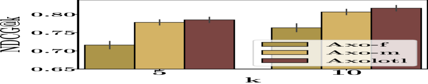
(a) CA $\rightarrow$ WA (40%)

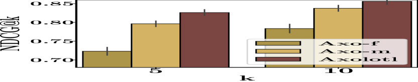
(b) TY $\rightarrow$ AI (40%)

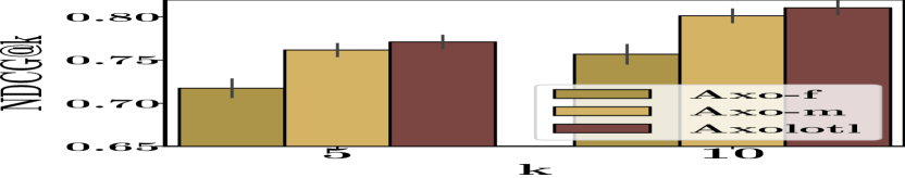
(c) NR $\rightarrow$ BE (40%)

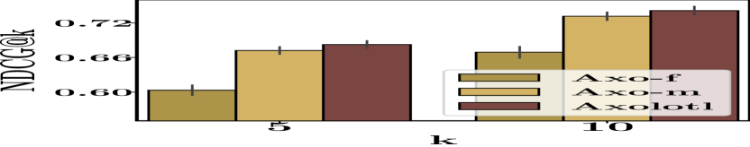
(d) CA $\rightarrow$ WA (60%)

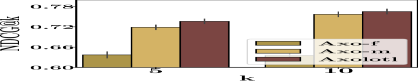
(e) TY $\rightarrow$ AI (40%)

(f) NR $\rightarrow$ BE (60%)

Figure 5. Analysis of Axolotl and its variants across different sizes of training data for both $\boldsymbol{\mathcal{D}}^{src}$ and $\boldsymbol{\mathcal{D}}^{tgt}$. Since the results are transductive, i.e. we only predict for users and locations present during training, they are specific to the subset of train-data.

5.4. Ablation Study (RQ2)

We conduct an ablation study for two key contributions in Axolotl: user-GATs ($\Phi_{1}$ and $\Phi_{2}$) and location-GATs ($\Phi_{3}$ and $\Phi_{4}$). For estimating the contribution of user-GATs, we use the meta-learning and alignment loss based training only for $\Phi_{1}$ and $\Phi_{2}$. We denote this variant as Axolotl-$\Phi_{1,2}$. Similarly for location-GATs we use Axolotl-$\Phi_{3,4}$. We also include a GCN (Kipf and Welling, 2017) based implementation of Axolotl denoted as Axolotl-gcn. From the results in Figure 6, we observe that Axolotl with joint training of user and location GATs has better prediction performance than Axolotl-$\Phi_{1,2}$ and Axolotl-$\Phi_{3,4}$. Interestingly, transferring across users leads to better prediction performance than transferring across locations. This could be attributed to a larger difference in the number of locations between source and target regions in comparison to the number of users. Axolotl-gcn has significant performance improvements over the preceding approaches with Axolotl further having modest improvements due to weighted neighborhood aggregation.

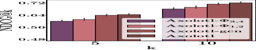
(a) Washington (US)

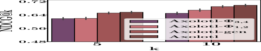
(b) Aizu (JP)

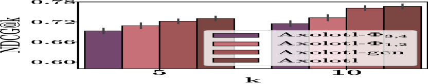
(c) Berlin (DE)

Figure 6. Ablation Study across different graph architectures possible in Axolotl along with a GCN variant.

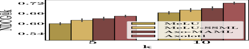
(a) Washington (US)

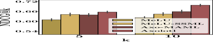
(b) Aizu (JP)

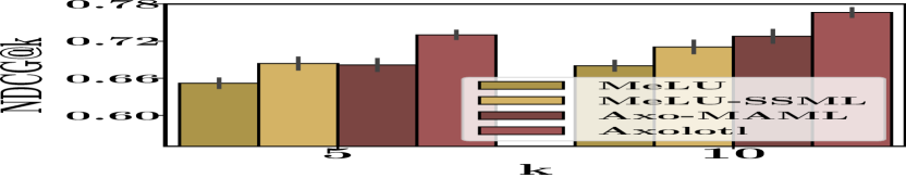
(c) Berlin (DE)

Figure 7. Contribution of novel spatio-social meta-learning in Axolotl and the corresponding gains over MeLU.

Contribution of SSML: To further assert the importance of our SSML (Section 4.3.1), we compare the state-of-the-art MAML-based model, viz., MeLU, with our proposed learning procedure, and also include results after training Axo-basic with MAML. From the results given in Figure 7, we note that MeLU, when trained with SSML, easily outperforms its MAML based counterpart. It not only demonstrates the effectiveness of the proposed learning method, but also its versatility to be incorporated with other baselines. This claim is substantiated further by the poorer performance of Axo-basic with MAML over the complete Axolotl model.

5.5. Transfer of Weights across Regions (RQ3)

Another important contribution we make in this paper is the cross-region transfer via cluster-based alignment loss. We show that Axolotl encapsulates the cluster-wise analogy by plotting the attention-weights corresponding to the similarity between location clusters ($\mathbf{L}^{tgt}_{c}$ and $\mathbf{L}^{src}_{c}$). We quantify the similarity using Damerau-Levenshtein distance (Contributors, 2021a) across category distribution for all clusters in source and target regions. Later, we group them into five equal buckets as per their similarity score, i.e. bucket-5 will have clusters with higher similarity as compared to other buckets. Figure 8 shows the mean attention value across each bucket for all datasets. We observe that Axolotl is able to capture the increase in inter-cluster similarity by increasing its attention weights. This feature is more prominent for Aizu and comparable for Berlin.

(a) Washington (US)

(b) Aizu (JP)

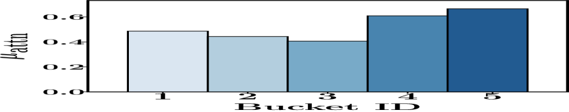
(c) Berlin (DE)

Figure 8. Bucket-wise Mean Attention Transfer Weights between Source and Target regions.

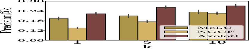
(a) Washington (US)

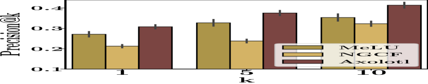
(b) Aizu (JP)

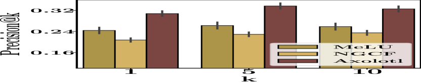
(c) Berlin (DE)

Figure 9. Recommending candidate POIs to a new user in the network i.e. with no past check-in records.

5.6. Prediction Performance for New Users

Though the focus of this paper is recommending locations to existing users, we perform an auxiliary cold-start recommendation experiment where we recommend candidate locations for users unseen in the training set. In this case, we obtain the final user embedding $\boldsymbol{U}_{f}$ of a new user based on her social network by avg-pooling (Hamilton et al., 2017). We compare this with the state-of-the-art recommender system, i.e. MeLU (Lee et al., 2019a) and NGCF (Wang et al., 2019b). From the results in terms for precision at different thresholds in Figure 9, we note that Axolotl performs significantly better than the other approaches, thus demonstrating that Axolotl is more suitable for POI recommendation even for a user with no past check-in records. We also note that MeLU easily outperforms NGCF and thus it further reinforces the need to incorporate out-of-region data for designing recommendation systems.

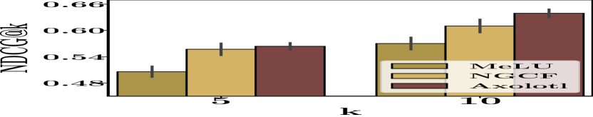
(a) California (US)

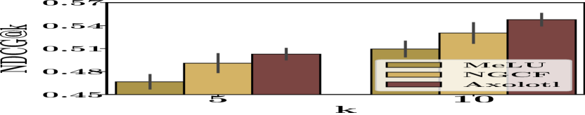
(b) Tokyo (JP)

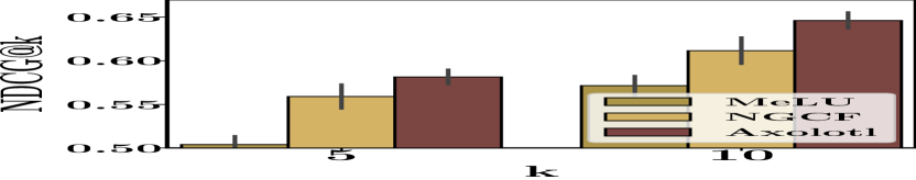
(c) North-Rhine Westphalia (DE)

Figure 10. Recommendation performance of Axolotl, NGCF and MeLU for users in the source region.

5.7. Axolotl for Source Regions

We also report the recommendation performance of Axolotl across different source regions, i.e. California(CA), Tokyo(TY), and North-Rhine Westphalia (NR). Here as well, we compare our model with MeLU (Lee et al., 2019a) and NGCF (Wang et al., 2019b). From the results in in Figure  10, we note that even when recommending for users in the source region, Axolotl performs comparable, if not better, than the state-of-the-art single region baseline NGCF. The results further support the practical usability of Axolotl even in data-rich source regions over its ability for limited data regions. We also note that for a source region, the performance of MeLU is significantly inferior than the other two approaches.

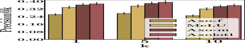
(a) Washington (GOW$\rightarrow$FSQ)

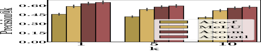
(b) Aizu (FSQ$\rightarrow$GOW)

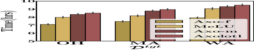
(c) Training Times

Figure 11. Cross-dataset recommendation performance for regions (a) Washington and (b) Aizu. (c) Training times of MeLU and different variants of Axolotl for all target datasets from the US.

5.8. Additional Experiments and Runtime

Transfer across Datasets: Finally, to further signify the ability of Axolotl to even work across different datasets, we design a novel task wherein we use the check-in data from Foursquare(FSQ) and Gowalla(GOW) for a specific region, train on the data-rich variant then later test on the data-scarce variant. Specifically we perform two more experiments of (i) training our model on Gowalla (1.8k Users, 15k POIs) derived section of Washington and predicted on its Foursquare(0.6k Users, 5.2k POIs) variant, and (ii) training on Foursquare(1.9k Users, 3.4k POIs) derived variant of Aizu and test on the Gowalla(0.9k Users, 1.7k POIs) variant. In contrast to the original datasets in Table 2, here we use a more lenient criteria to filter out unnecessary users and locations, with each user having more than 2 check-ins, 2 social connections and each location with more than 3 check-ins. We plot the results for Washington and Aizu in Figure 11(a) and Figure 11(b) respectively. From the results we note that a standard fine tuning-based model Axo-f is not suitable for transferring across different datasets. However, meta-learning based models such as MeLU, Axo-m and Axolotl perform significantly better. We also note that even when predicting across different datasets, Axolotl considerably outperforms MeLU across all metrics.

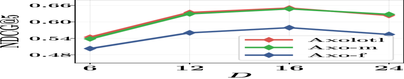
(a) Across Hidden Dimension

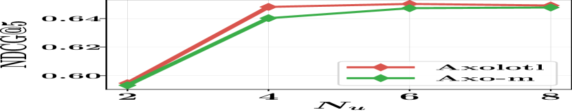
(b) No. of target region updates

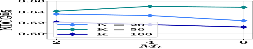
(c) Across $K$ and $M_{t}$

Figure 12. Axolotl sensitivity across for WA dataset. Since fig(c) only considers varying cluster sizes, we omit performance of other Axolotl variants and report only on the complete Axolotl model.

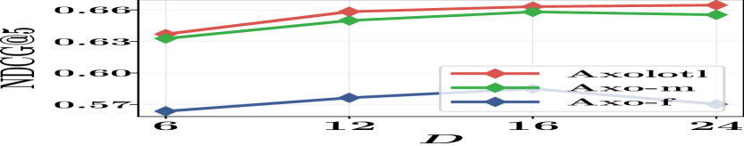
(a) Across Hidden Dimension

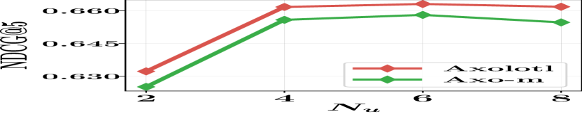
(b) No. of target region updates

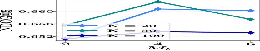
(c) Across $K$ and $M_{t}$

Figure 13. Axolotl sensitivity across for AI dataset. Following Figure 12, we only report the results of the complete Axolotl model in fig (c).

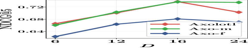
(a) Across Hidden Dimension

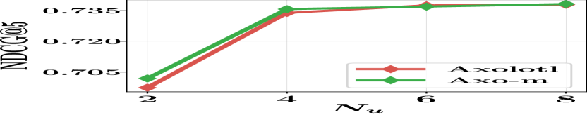
(b) No. of target region updates

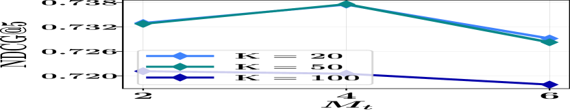
(c) Across $K$ and $M_{t}$

Figure 14. Axolotl sensitivity across for BE dataset. Following Figure 12, we only report the results of the complete Axolotl model in fig (c).

Runtime Analysis: We also report on the run-time of Axolotl to verify its applicability in real-world settings. We report the run-times for Axolotl over the largest datasets, i.e. the states in the U.S. CA(42.1k POIs) $\rightarrow$ WA(16.7k POIs), MA(10.5k POIs), OH(8.5k POIs). From the results in Figure  11(c), we note that even for transferring across largest dataset, i.e Washington, the overall training time of Axolotl on a Tesla V100 GPU is comparable to those of MeLU. We also highlight that these differences were even lower in smaller datasets which we exclude for brevity. Though the training times are feasible for deployment, the large run-time is mainly due to the inefficient CPU based batch-sampling. With a GPU-based sampling alternatives (Chen et al., 2018; Ramezani et al., 2020; Auten et al., 2020), this run-time can be significantly improved which we consider as a future work. Though the current single-threaded sampling affects the training time of Axolotl, the time-taken (in seconds) for inference, being: 3.27, 3.19, and 5.74 for Aizu, Berlin and Washington respectively, are well within range for practical deployment. We also note that the cluster-alignment loss improves the prediction performance of Axolotl and yet includes a minor computation cost over the meta-learning variant Axo-m.

5.9. Parameter Sensitivity (RQ4)

Finally, we perform the sensitivity analysis of Axolotl over key parameters: (1) $D$, the dimension of embeddings; (2) $N_{u}$, no. of meta-updates on a target batch before a source batch update; (3) $M_{t}$, epochs after which we initiate cluster based transfer; and (4) $K$, no. of clusters for source and target (see Table 1). We report the results for WA, AI and BE in Figure 12, 13, and 14 respectively. We note that as we increase the embedding dimension the performance first increases since it leads to better modeling. However, beyond a point, the complexity of the model increases requiring more training to achieve good results, and hence we see its performance deteriorating. Across $N_{u}$, we note that increasing the number of updates with batches from the target region leads to better results before saturating at a certain point. We found $N_{u}=4$ to be the optimal point across datasets in our experiments. Across $M_{t}$, we notice that a delayed transfer based on clusters leads to a degradation in performance. This could be attributed to the saturation of parameters due to continuous updates through meta-learning iterations. Finally across $K$, we observe the presence of an optimal number of clusters for the source and target regions. Specifically, increasing $K$ leads to a better recommendation performance as it provides higher flexibility to POI and users with similar characteristics to be assigned the same cluster while simultaneously discarding the noisy entities. However, we note that beyond a certain threshold the performance deteriorates as it reduces the variance between clusters and creates artificial boundaries within similar clusters.

6. Conclusion

In conclusion, we developed a novel architecture called Axolotl that incorporates mobility data from other regions to design a location recommendation system for data-scarce regions. We also propose a novel procedure called spatio-social meta learning approach that captures the regional mobility patterns as well as the graph structure. We address the problems associated with an extremely data-scarce region and devise a suitable cluster-based alignment loss that enforce similar embeddings for communities of user and locations with similar dynamics. Our novel graph attention based model captures the complex user-location influence patterns for a specific region. Experiments over diverse mobility datasets revealed that Axolotl is able to significantly improve over the state-of-the-art baselines for POI recommendation in limited data regions and even performs considerably better across datasets and data-rich source regions. As a future work for this paper, we plan to modify the transfer procedure of Axolotl to incorporate novel meta-learning approaches, namely ProtoMAML (Triantafillou et al., 2020) and Reptile (Nichol et al., 2018). Additionally, we plan to experiment with approaches (Lee et al., 2019b; Ying et al., 2018b; Chen et al., 2021) that automatically identify the number of clusters within a region while simultaneously maintaining the scalability of our model.

- (1)
- Abu-El-Haija et al. (2019) Sami Abu-El-Haija, Bryan Perozzi, Amol Kapoor, Nazanin Alipourfard, Kristina Lerman, Hrayr Harutyunyan, Greg Ver Steeg, and Aram Galstyan. 2019. Mixhop: Higher-order graph convolutional architectures via sparsified neighborhood mixing. In ICML.
- Auten et al. (2020) Adam Auten, Matthew Tomei, and Rakesh Kumar. 2020. Hardware acceleration of graph neural networks. In DAC.
- Barkhuus and Dey (2003) Louise Barkhuus and Anind K Dey. 2003. Location-Based Services for Mobile Telephony: a Study of Users Privacy Concerns. In Interact.
- Bharadhwaj (2019) Homanga Bharadhwaj. 2019. Meta-Learning for User Cold-Start Recommendation. In IJCNN.
- Bottou et al. (2018) Léon Bottou, Frank E Curtis, and Jorge Nocedal. 2018. Optimization methods for large-scale machine learning. Siam Review (2018).
- Chakraborty et al. (2020) Anirban Chakraborty, Debasis Ganguly, and Owen Conlan. 2020. Relevance Models for Multi-Contextual Appropriateness in Point-of-Interest Recommendation. In SIGIR.
- Chen et al. (2018) Jie Chen, Tengfei Ma, and Cao Xiao. 2018. FastGCN: Fast Learning with Graph Convolutional Networks via Importance Sampling. In ICLR.
- Chen et al. (2021) Ling Chen, Jiahui Xu, Binqing Wu, Yuntao Qian, Zhenhong Du, Yansheng Li, and Yongjun Zhang. 2021. Group-Aware Graph Neural Network for Nationwide City Air Quality Forecasting. arXiv preprint arXiv:2108.12238 (2021).
- Cheng et al. (2013) Chen Cheng, Haiqin Yang, Michael R Lyu, and Irwin King. 2013. Where you like to go next: Successive point-of-interest recommendation. In IJCAI.
- Cho et al. (2011) Eunjoon Cho, Seth A. Myers, and Jure Leskovec. 2011. Friendship and mobility: User movement in location-based social networks. In KDD.
- Christoforidis et al. (2021) Giannis Christoforidis, Pavlos Kefalas, Apostolos N Papadopoulos, and Yannis Manolopoulos. 2021. RELINE: Point-of-interest recommendations using multiple network embeddings. Knowledge and Information Systems (2021).
- Contributors (2021a) Wikipedia Contributors. 2021a. Damerau Levenshtein distance. Available At: https://en.wikipedia.org/wiki/Damerau_Levenshtein_distance.
- Contributors (2021b) Wikipedia Contributors. 2021b. Haversine formula. Available At: https://en.wikipedia.org/wiki/Haversine_formula.
- Dong et al. (2020) Manqing Dong, Feng Yuan, Lina Yao, Xiwei Xu, and Liming Zhu. 2020. MAMO: Memory-Augmented Meta-Optimization for Cold-Start Recommendation. In KDD.
- Fan et al. (2019) Wenqi Fan, Yao Ma, Qing Li, Yuan He, Eric Zhao, Jiliang Tang, and Dawei Yin. 2019. Graph Neural Networks for Social Recommendation. In WWW.
- Fan et al. (2016) Zipei Fan, Xuan Song, Ryosuke Shibasaki, Tao Li, and Hodaka Kaneda. 2016. CityCoupling: Bridging Intercity Human Mobility. In UbiComp.
- Feng et al. (2018) Jie Feng, Yong Li, Chao Zhang, Funing Sun, Fanchao Meng, Ang Guo, and Depeng Jin. 2018. DeepMove: Predicting Human Mobility with Attentional Recurrent Networks. In WWW.
- Finn et al. (2017) Chelsea Finn, Pieter Abbeel, and Sergey Levine. 2017. Model-agnostic meta-learning for fast adaptation of deep networks. In ICML.
- Gao and Ji (2019) Hongyang Gao and Shuiwang Ji. 2019. Graph U-Nets. In ICML.
- Glueck (2019) Jeff Glueck. 2019. The Future of Location Technology. Available At: https://bit.ly/2VWrABc.
- Grover and Leskovec (2016) Aditya Grover and Jure Leskovec. 2016. node2vec: Scalable Feature Learning for Networks. In KDD.
- Guo et al. (2019) Shengnan Guo, Youfang Lin, Ning Feng, Chao Song, and Huaiyu Wan. 2019. Attention based spatial-temporal graph convolutional networks for traffic flow forecasting. In AAAI.
- Gupta and Bedathur (2021) Vinayak Gupta and Srikanta Bedathur. 2021. Region Invariant Normalizing Flows for Mobility Transfer. In CIKM.
- Gupta et al. (2021) Vinayak Gupta, Abir De, Sourangshu Bhattacharya, and Srikanta Bedathur. 2021. Learning Temporal Point Processes with Intermittent Observations. In AISTATS.
- Hamilton et al. (2017) Will Hamilton, Zhitao Ying, and Jure Leskovec. 2017. Inductive representation learning on large graphs. In NeurIPS.
- Hao et al. (2021) Bowen Hao, Jing Zhang, Hongzhi Yin, Cuiping Li, and Hong Chen. 2021. Pre-Training Graph Neural Networks for Cold-Start Users and Items Representation. In WSDM.
- He et al. (2020) Tianfu He, Jie Bao, Ruiyuan Li, Sijie Ruan, Yanhua Li, Li Song, Hui He, and Yu Zheng. 2020. What is the Human Mobility in a New City: Transfer Mobility Knowledge Across Cities. In WWW.
- He et al. (2017a) Xiangnan He, Ming Gao, Min-Yen Kan, and Dingxian Wang. 2017a. BiRank: Towards Ranking on Bipartite Graphs. arXiv preprint arXiv:1708.04396 (2017).
- He et al. (2017b) Xiangnan He, Lizi Liao, Hanwang Zhang, Liqiang Nie, Xia Hu, and Tat-Seng Chua. 2017b. Neural Collaborative Filtering. In WWW.
- Jang et al. (2019) Yunhun Jang, Hankook Lee, Sung Ju Hwang, and Jinwoo Shin. 2019. Learning What and Where to Transfer. In ICML.
- Kipf and Welling (2017) Thomas N. Kipf and Max Welling. 2017. Semi-supervised classification with graph convolutional networks. In ICLR.
- Krishnan et al. (2020) Adit Krishnan, Mahashweta Das, Mangesh Bendre, Hao Yang, and Hari Sundaram. 2020. Transfer Learning via Contextual Invariants for One-to-Many Cross-Domain Recommendation. In SIGIR.
- Lee et al. (2019a) Hoyeop Lee, Jinbae Im, Seongwon Jang, Hyunsouk Cho, and Sehee Chung. 2019a. MeLU: Meta-Learned User Preference Estimator for Cold-Start Recommendation. In KDD.
- Lee et al. (2017) Jaekoo Lee, Hyunjae Kim, Jongsun Lee, and Sungroh Yoon. 2017. Transfer Learning for Deep Learning on Graph-Structured Data. In AAAI.
- Lee et al. (2019b) Junhyun Lee, Inyeop Lee, and Jaewoo Kang. 2019b. Self-attention graph pooling. In ICML.
- Li et al. (2018a) Hui Li, Ke Deng, Jiangtao Cui, Zhenhua Dong, Jianfeng Ma, and Jianbin Huang. 2018a. Hidden community identification in location-based social network via probabilistic venue sequences. Information Sciences (2018).
- Li and Tuzhilin (2020) Pan Li and Alexander Tuzhilin. 2020. DDTCDR: Deep Dual Transfer Cross Domain Recommendation. In WSDM.
- Li et al. (2019) Ruirui Li, Jyunyu Jiang, Chelsea Ju, and Wei Wang. 2019. CORALS: Who are My Potential New Customers? Tapping into the Wisdom of Customers Decisions. In WSDM.
- Li et al. (2020) Ruirui Li, Xian Wu, Xiusi Chen, and Wei Wang. 2020. Few-Shot Learning for New User Recommendation inLocation-based Social Networks. In WWW.
- Li et al. (2018b) Yaguang Li, Rose Yu, Cyrus Shahabi, and Yan Liu. 2018b. Diffusion Convolutional Recurrent Neural Network: Data-Driven Traffic Forecasting. In ICLR.
- Likhyani et al. (2017) Ankita Likhyani, Srikanta Bedathur, and Deepak P. 2017. LoCaTe: Influence Quantification for Location Promotion in Location-based Social Networks. In IJCAI.
- Likhyani et al. (2020) Ankita Likhyani, Vinayak Gupta, PK Srijith, P Deepak, and Srikanta Bedathur. 2020. Modeling Implicit Communities from Geo-tagged Event Traces using Spatio-Temporal Point Processes. In WISE.
- Liu et al. (2016) Qiang Liu, Shu Wu, Liang Wang, and Tieniu Tan. 2016. Predicting the Next Location: A Recurrent Model with Spatial and Temporal Contexts. In AAAI.
- Lu et al. (2020) Yuanfu Lu, Yuan Fang, and Chuan Shi. 2020. Meta-learning on Heterogeneous Information Networks for Cold-start Recommendation. In KDD.
- Manotumruksa et al. (2018) Jarana Manotumruksa, Craig Macdonald, and Iadh Ounis. 2018. A Contextual Attention Recurrent Architecture for Context-Aware Venue Recommendation. In SIGIR.
- Manotumruksa et al. (2019) Jarana Manotumruksa, Dimitrios Rafailidis, Craig Macdonald, and Iadh Ounis. 2019. On Cross-Domain Transfer in Venue Recommendation. In ECIR.
- Morris et al. (2019) Christopher Morris, Martin Ritzert, Matthias Fey, William L Hamilton, Jan Eric Lenssen, Gaurav Rattan, and Martin Grohe. 2019. Weisfeiler and leman go neural: Higher-order graph neural networks. In AAAI.
- Nichol et al. (2018) Alex Nichol, Joshua Achiam, and John Schulman. 2018. On First-Order Meta-Learning Algorithms. arXiv preprint arXiv 1803.02999 (2018).
- Noulas et al. (2011) Anastasios Noulas, Salvatore Scellato, Cecilia Mascolo, and Massimiliano Pontil. 2011. Exploiting semantic annotations for clustering geographic areas and users in location-based social networks. In The Social Mobile Web, ICWSM Workshop.
- Ouyang et al. (2018) Kun Ouyang, Reza Shokri, David S Rosenblum, and Wenzhuo Yang. 2018. Non-Parametric Generative Model for Human Trajectories. In IJCAI.
- Pan et al. (2019) Zheyi Pan, Yuxuan Liang, Weifeng Wang, Yong Yu, Yu Zheng, and Junbo Zhang. 2019. Urban Traffic Prediction from Spatio-Temporal Data Using Deep Meta Learning. In KDD.
- Ramezani et al. (2020) Morteza Ramezani, Weilin Cong, Mehrdad Mahdavi, Anand Sivasubramaniam, and Mahmut Kandemir. 2020. GCN meets GPU: Decoupling ”When to Sample” from ”How to Sample” Observations. In NeurIPS.
- Rendle (2010) Steffen Rendle. 2010. Factorization machines. In ICDM.
- Scellato et al. (2011) Salvatore Scellato, Anastasios Noulas, and Cecilia Mascolo. 2011. Exploiting place features in link prediction on location-based social networks. In KDD.
- Singh and Gordon (2008) Ajit P Singh and Geoffrey J Gordon. 2008. Relational learning via collective matrix factorization. In KDD.
- Triantafillou et al. (2020) E. Triantafillou, T. Zhu, V. Dumoulin, P. Lamblin, U. Evci, K. Xu, R. Goroshin, C. Gelada, K. Swersky, P. Manzagol, and H. Larochelle. 2020. Meta-Dataset: A Dataset of Datasets for Learning to Learn from Few Examples. In ICLR.
- Vartak et al. (2017) Manasi Vartak, Arvind Thiagarajan, Conrado Miranda, Jeshua Bratman, and Hugo Larochelle. 2017. A Meta-Learning Perspective on Cold-Start Recommendations for Items. In NeurIPS.
- Vaswani et al. (2017) Ashish Vaswani, Noam Shazeer, Niki Parmar, Jakob Uszkoreit, Llion Jones, Aidan N Gomez, Łukasz Kaiser, and Illia Polosukhin. 2017. Attention is all you need. In NeurIPS.
- Veličković et al. (2018) Petar Veličković, Guillem Cucurull, Arantxa Casanova, Adriana Romero, Pietro Liò, and Yoshua Bengio. 2018. Graph Attention Networks. In ICLR.
- Wang et al. (2019a) Leye Wang, Xu Geng, Xiaojuan Ma, Feng Liu, and Qiang Yang. 2019a. Cross-city transfer learning for deep spatio-temporal prediction. In IJCAI.
- Wang et al. (2019b) Xiang Wang, Xiangnan He, Meng Wang, Fuli Feng, and Tat-Seng Chua. 2019b. Neural Graph Collaborative Filtering. In SIGIR.
- Wang et al. (2012) Zhu Wang, Daqing Zhang, Dingqi Yang, Zhiyong Yu, and Xingshe Zhou. 2012. Detecting overlapping communities in location-based social networks. In SocInfo.
- Wei et al. (2016) Ying Wei, Yu Zheng, and Qiang Yang. 2016. Transfer knowledge between cities. In KDD.
- Wu et al. (2017) Hao Wu, Ziyang Chen, Weiwei Sun, Baihua Zheng, and Wei Wang. 2017. Modeling trajectories with recurrent neural networks. In IJCAI.
- Wu et al. (2016) Le Wu, Yong Ge, Qi Liu, Enhong Chen, Bai Long, and Zhenya Huang. 2016. Modeling users preferences and social links in social networking services: A joint-evolving perspective. In AAAI.
- Wu et al. (2019b) Qitian Wu, Hengrui Zhang, Xiaofeng Gao, Peng He, Paul Weng, Han Gao, and Guihai Chen. 2019b. Dual Graph Attention Networks for Deep Latent Representation of Multifaceted Social Effects in Recommender Systems. In WWW.
- Wu et al. (2019a) Yongji Wu, Defu Lian, Shuowei Jin, and Enhong Chen. 2019a. Graph Convolutional Networks on User Mobility Heterogeneous Graphs for Social Relationship Inference. In IJCAI.
- Yang et al. (2019) Dingqi Yang, Bingqing Qu, Jie Yang, and Philippe Cudre-Mauroux. 2019. Revisiting User Mobility and Social Relationships in LBSNs: A Hypergraph Embedding Approach. In WWW.
- Yao et al. (2019a) Huaxiu Yao, Yiding Liu, Ying Wei, Xianfeng Tang, and Zhenhui Li. 2019a. Learning from Multiple Cities: A Meta-Learning Approach for Spatial-Temporal Prediction. In WWW.
- Yao et al. (2019b) Huaxiu Yao, Ying Wei, Junzhou Huang, and Zhenhui Li. 2019b. Hierarchically Structured Meta-learning. In ICML.
- Yao et al. (2020) Huaxiu Yao, Chuxu Zhang, Ying Wei, Meng Jiang, Suhang Wang, Junzhou Huang, and Nitesh V. Chawla. 2020. Graph Few-shot Learning via Knowledge Transfer. In AAAI.
- Ying et al. (2018a) Rex Ying, Ruining He, Kaifeng Chen, Pong Eksombatchai, William L Hamilton, and Jure Leskovec. 2018a. Graph convolutional neural networks for web-scale recommender systems. In KDD.
- Ying et al. (2018b) Rex Ying, Jiaxuan You, Christopher Morris, Xiang Ren, William L Hamilton, and Jure Leskovec. 2018b. Hierarchical graph representation learning with differentiable pooling. In NeurIPS.
- Zagoruyko and Komodakis (2017) Sergey Zagoruyko and Nikos Komodakis. 2017. Paying more attention to attention: Improving the performance of convolutional neural networks via attention transfer. In ICLR.
- Zhang et al. (2019) Yunchao Zhang, Yanjie Fu, Pengyang Wang, Yu Zheng, and Xiaolin Li. 2019. Unifying Inter-Region Autocorrelations and Intra-Region Structure for Spatial Embedding via Collective Adversarial Learning. In KDD.
- Zheng (2011) Yu Zheng. 2011. Location-Based Social Networks: Users. In Computing with Spatial Trajectories. 243–276.
- Zhuang and Ma (2018) Chenyi Zhuang and Qiang Ma. 2018. Dual Graph Convolutional Networks for Graph-Based Semi-Supervised Classification. In WWW.