Element abundances in metal poor local star-forming galaxies constrained by the weak spectral lines

We have collected from different surveys some significant spectroscopic data observed from star-forming galaxies in the local Universe. The objects showing a relatively rich spectrum in number of lines from different elements were selected in order to constrain the models. In particular, we looked at the relatively weak lines such as [OIII]4363, HeII4686, HeI4471 and HeI5876. We have modelled in detail the spectra by the coupled effect of photoionization from the stars and shocks. We have found that the abundances relative to H of most of the elements are lower than solar but not as low as those evaluated by the direct strong line and the $\rm T_{e}$ methods. Sulphur which appears through the [SII]6717,6731 and [SIII]6312 lines is not depleted, revealing a strong contribution from the ISM. We have added to the sample the optical-UV spectra of local low-metallicity dwarf galaxies containing the CIV/H${\beta}$  and CIII]/H${\beta}$  line ratios in order to determine with relative precision the C/H relative abundance. The results show He/H lower than solar in some objects and suggest that the geometrical thickness of the clouds constrains the HeII/H${\beta}$  line ratios. We explain the low He/H by mixing of the wind from the star-forming region with ISM clouds.

1 Introduction

The transformation of the line spectra emitted from galaxies throughout the redshift is a leading argument because it is connected with reionization at a certain epoch (Izotov et al 2020 and references therein). In local galaxies, however, the reionization era is less directly recognized from the element abundances because of physical and chemical phenomena acting on gas and dust, respectively, in their evolution towards the local era. Even for high redshift galaxy spectra Rupke et al (2005) claim that ’the prominence of Ly$\alpha$ makes it a tempting target for parametrizing outflows. However, radiation transfer effects make it an ambiguous indicator.’

In this paper we deal with the spectra emitted from local star-forming (SF) galaxies. In the latest years, the number of lines that could be observed in each spectrum from local galaxies substantially increased. In fact, the observations (e.g. Izotov et al 1997, 2006, 2018a,b, 2019a,b, 2021, Guseva et al 2020, Pérez-Montero et al 2005, Pustilnik et al 2004, Berg et al 2012, 2016, etc.) provide high precision spectra accounting for significant lines in the optical– near-IR range which are generally weak ([OIII]4363, HeII 4684, HeI 5876, [OI]6300,6363, [SIII]6312, etc.) besides the relatively strong [NeIII]3869,3969, [OIII]5007,4959, [OII]3727,3729, [NII]6548,6584, [SII]6717, 6731 doublets and the Balmer H${\alpha}$  and H${\beta}$  lines. Berg et al (2016) presented high precision spectra accounting also for UV lines, in particular CIV1548,1550 and CIII]1906, 1909. The weak lines that appear in nearly all local galaxy surveys allow a more accurate classification of galaxy types such as AGN, starburst and host galaxies in general. For galaxy surveys at high redshift z$>$1 the strongest lines which are provided by the observations are necessarly sufficient to obtain the characteristic physical conditions of the gas although with some uncertainty (see e.g. Contini 2014 and references therein).

The increasing number of objects observed in recent surveys demands fast classification methods dictated directly by the observations such as e.g. the BPT diagrams (Baldwin, Phillips & Terlevich 1981, Kauffmann 2003, Kewley 2001) for AGN, star-formation and shock dominated objects. Most authors use the $\rm T_{e}$ method that was succesfully adopted for AGN (e.g. Monteiro & Dors 2021 and references therein). Direct methods such as the $\rm T_{e}$ ones and those based on the strong lines and on the electron temperature and density obtained from the characteristic line ratios (e.g. Izotov et al 2020, 2021 and references therein) yield metallicity results (in terms in particular of the O/H relative abundance) for single objects with a relatively high precision. By these methods very low element abundances compared to solar were generally found in local star-forming galaxies (SFG) and HII regions, while abundances less far from solar in objects at similar redshifts were found by the detailed modelling of the spectra (e.g. Contini 2017 and references therein). However, detailed modelling methods are long-time spending even when used to fit a single spectrum therefore, they are less adapted to model surveys presenting a high number of galaxy spectra.

Detailed modelling methods were used to investigate AGN spectra (e.g. cloudy, Ferland et al 2017). They can be adapted to distinguish the spectra emitted from gas affected by the flux from different photoionization sources. However, models based on pure photoionization cannot always reproduce all the lines in a single spectrum. For instance, in some spectra emitted from SFG the HeII4686 line is evident. In order to reproduce the observed HeII/H${\beta}$  line ratio the emitting gas should be heated to a relatively high temperature because the ionization potential of the He⁺⁺ ion is relatively high (54.17 eV). Therefore, in the present investigation we use the code suma (e.g. Contini 2009) which shows the role of shocks coupled to the photoionization flux. To reproduce the spectra emitted from local SF galaxies, shocks propagating throughout a ionized medium with a relatively high velocity (300-500 $\rm km\,s^{-1}$) were proposed by Izotov et al (2012) in order to heat the gas to temperatures high enough to obtain strong HeII4686 lines. Shocks propagating throughout a neutral medium, on the other hand, were suggested by Allen et al (2008).

In this paper we present the method adopted to evaluate the abundances of the leading elements in local SFG and we compare our results with those obtained by the $\rm T_{e}$ and strong line methods. We have selected the spectra more adapted to modelling, i.e. those containing at least H${\beta}$, H${\alpha}$, [OIII]5007, [OII]3727 and the [NII] lines. We have chosen to explore in particular local SFG spectra characterized by significantly high [OIII]5007/[OII]3727 ($>$ 10) and low [OII]3727/H${\beta}$  ($\leq$1), [NII]/H${\beta}$, [SII]/H${\beta}$  and [OI]/H${\beta}$, as those presented by Izotov et al (2020), Izotov et al (2019a,b), Izotov et al (2018a,b,), Guseva et al (2020), Pustilnik et al (2004), etc. The sample of galaxies selected in this paper is presented in Sect. 2. Results are given in Sect. 3 and discussed in Sect. 4. Concluding remarks follow in Sect. 5.

2 Selected galaxies

The SFG sample selected for our investigation is shown in Table 1. Each galaxy is presented by the corresponding redshift, by the observed H${\beta}$  line intensity, the observed H${\alpha}$/H${\beta}$  and H${\gamma}$/H${\beta}$  line ratios. The corresponding calculated values are reported from the next sections. These Balmer lines were chosen because a) from the comparison of calculated with observed H${\beta}$  the radius of the emitting nebulae can be evaluated, b) from the comparison of the calculated with observed H${\alpha}$/H${\beta}$  the physical conditions in the emitting nebulae are roughly evaluated and c) from the comparison of calculated with observed H${\gamma}$/H${\beta}$  line blending can be revealed.

The SFG sample includes the galaxies of the Izotov et al (2020, hereafter I20) survey which covers the 0.02811$\leq$z$\leq$0.06360 redshift range. The spectra were classified as extremely metal-poor types. The survey contains eight objects with similar line ratios except for [OIII]5007+/H${\beta}$  (the plus indicates that the 5007, 4959 doublet is summed) which ranges between 5.49 and 10.35. Moreover, the [OII]3727+3729/H${\beta}$  ratios are as low as the [OIII]4363/H${\beta}$  ones. Characteristic of these spectra are the HeI4471 and HeII4686 lines which are often lacking in SFG spectra. We have added to the I20 survey the spectrum of the most metal-poor galaxy J1234+3901 at z=0.133 presented by Izotov et al (2019b, hereafter I19b) which shows a relatively low [OIII]5007+/H${\beta}$=2.7, for comparison. J0811+4730 spectrum presented by Izotov et al (2018a hereafter I18a) at z=0.04444 contains the HeII line. I18a found an extremely low metallicity (12+log(O/H)=6.98). J0811+4730 is also included in our sample (Table 1). Moreover, the survey of SFG presented by Izotov et al (2018b, hereafter I18b) at z=0.2993-0.4317 with relatively high [OIII]5007+/[OII]3727+ (but lower than those included in the I20 survey) is also accounted for. I18b observations were aimed to detect Lyman continuum emission. I18b claim that they discovered ’a class of galaxies in the local Universe which are leaking ionizing radiation and sharing many properties of high-redshift galaxies’. I18b have found very low metallicities by the strong line methods. They suggest about local SFG galaxies with low metallicities that a considerable fraction of the galaxy stellar mass was formed during the most recent burst of star formation. Guseva et al (2020, hereafter G20) presented observations of SFG, in particular J0901+2119 and J1011+1947 already included within the I18b survey but containing more significant lines (e.g. MgII2796). We included the G20 survey in our sample.

Pérez-Montero et al (2011) observed blue compact dwarf (BCD) galaxies at z between 0.016 and 0.042 with the aim of investigating galaxies with an outstandingly high N/H relative abundance. The spectrum of one of these galaxies (HS0837.4717 at z=0.04195) - particularly rich in significant lines - was already observed by Pustilnik et al (2004, hereafter P04) with the same aim. It appears in our sample. Two galaxies, J0314-0108 (z=0.02027) and J1433+1544 (z=0.02741) were selected from the Izotov et al (2019a, hereafter I19a) survey which includes in the spectra the [OII]7327+ doublet, but it lacks some other lines such as e.g. the He ones. Unfortunately most of the spectra do not show all the significant lines, in particular the [OII]3727+. Therefore only two galaxies are added for comparison in our sample. Berg et al (2016) presented the spectra of selected metal poor local dwarf galaxies at z between 0.003 and 0.04 containing some characteristic UV lines (e.g. CIV and CIII]). We have included this survey in order to calculate the C/O and C/N relative abundances.

Table 1: Balmer lines

galaxy	z	H${\beta}$(obs)1	H${\beta}$(calc)2	H${\alpha}$/H${\beta}$(obs)	H${\alpha}$/H${\beta}$(calc)	H${\gamma}$/H${\beta}$(obs)	H${\gamma}$/H${\beta}$(calc)
J0007+02263	0.06360	52.3	120	2.77	2.84	0.473	0.47
J0159+07513	0.06105	99.3	4.	2.75	2.93	0.475	0.46
J0820+54313	0.03851	20.2	1.9	2.32	2.9	0.486	0.46
J0926+45043	0.04232	34.4	1.4	2.75	2.93	0.44	0.46
J1032+49193	0.04420	109.6	2.2	-	3.4	0.448	0.45
J1205+45513	0.06540	115.0	5.	2.75	3.27	0.475	0.42
J1242+48513	0.06226	40.1	2.	2.72	2.94	0.497	0.46
J1355+46513	0.02811	51.2	1.9	2.73	2.9	0.483	0.46
J1234+39014	0.13297	9.74	9.	2.71	3.18	0.46	0.45
J0901+21195,6	0.2993	29.1	36	2.88	2.88	0.48	0.46
J1011+19475,6	0.3322	27.0	4.2	2.83	2.88	0.445	0.465
J1243+46465	0.4317	14.1	5.1	2.8	2.95	0.47	0.462
J1248+42595	0.3629	35.2	4.6	2.79	2.95	0.496	0.461
J1256+45095	0.3530	11.4	5.7	2.80	2.9	0.482	0.464
J0925+14036	0.3010	21.61	30.0	2.85	2.9	0.47	0.46
J1154+24436	0.3690	9.77	3.7	2.77	2.92	0.45	0.46
J1442+02096	0.2937	19.44	7.0	2.82	2.84	0.47	0.47
J0811+47307	0.04444	12.60	7.	3.12	3.25	0.48	0.45
HS0837+47178	0.04195	313	90.	2.76	2.89	0.48	0.46
J0314-01089	0.02741	26.2	9.4	-	3.1	-	0.455
J1433+15449	0.02027	2.0	8.5	-	3.1	-	0.456
J08255510	0.003	230.811	2.6	2.76	2.96	0.476	0.46
J10445710	0.013	413.711	2.35	2.75	3.0	0.506	0.46
J12012210	0.003	114.311	0.8	2.78	2.96	0.53	0.46
J12415910	0.009	98.311	31.	2.79	2.97	0.495	0.46
J12262210	0.007	81.3111	10.	2.79	3.34	0.493	0.46
J12243610	0.040	138.411	1.7	2.79	3.26	0.458	0.45
J12482710	0.030	78.111	1.7	2.77	3.26	0.47	0.46

¹ in units of 10^-16 $\rm erg\,cm^{-2}\,s^{-1}$; ² in 10^-4 $\rm erg\,cm^{-2}\,s^{-1}$; ³ I20 survey; ⁴ I19b for J1234.3901; ⁵ I18b survey; ⁶ G20 survey ;⁷ I18a; ⁸ P04); ⁹ I19a survey; ¹⁰ B16 galaxy sample; ¹¹ observed flux in units of 10^-16 $\rm erg\,cm^{-2}\,s^{-1}$.

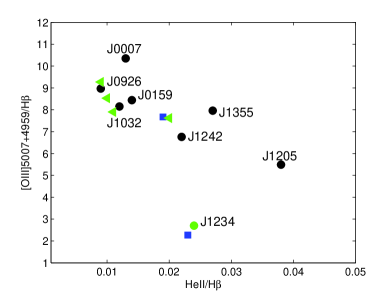
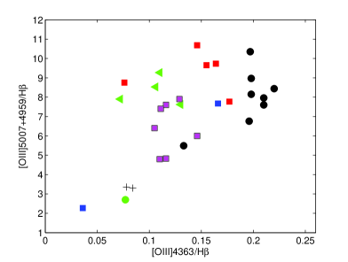
Figure 1: Black circles: I20 survey galaxies; green circle: J1234 (I19b); red squares: I18b survey objects; blue squares: J0811 (I18a) and HS0837 (P04); green triangles: G20 survey galaxies; black plus: I19a survey; magenta squares: B16

To have a first hint about the nature of the objects in our sample we present in Fig. 1 the correlations of some significant observed line ratios. The data come from Tables 2, 5, 7, 9 and 10. In the top diagram, [OIII]5007+/H${\beta}$  versus HeII/H${\beta}$  indicates that [OIII]5007+/H${\beta}$  increases when HeII/H${\beta}$  decreases. Generally, both [OIII]5007+/H${\beta}$  and HeII/H${\beta}$  should increase with the temperature of the emitting gas. Fig. 1 (top) clearly shows an opposite trend. This suggests that the emission lines come from a region within the cloud where the O³⁺ ion is relatively strong, in agreement with I20 claim. J1234 is dislocated from the general trend for perhaps two reasons. First, it was inserted in Table 2 because its spectrum shows the HeII line but this galaxy is at redshift z=0.133, while the I20 sample is at z$\leq$ between 0.028 and 0.0654. Second, the [OIII]5007+/H${\beta}$  ratio is the lowest observed one among the sample galaxies presented in Table 1. In fact, spectra with a relatively high [OIII]/H${\beta}$  were selected by I20. J0007, J1355 and J1205 are slightly shifted towards higher HeII/H${\beta}$. This could suggest that these galaxies belonging to the I20 survey correspond to quasi solar He/H ([He/H]_⊙=0.1). However, the trend is not only due to the He/H relative abundance. The other diagrams show that J0007 and J1205 correspond to different parameters on a large scale. [OIII]5007+/H${\beta}$  versus [OIII]4363/H${\beta}$  (Fig. 1, middle diagram) and [OIII]5007+/H${\beta}$  versus [OII]3727+/H${\beta}$  (bottom) confirm that in general the spectra do not depend on a single specific parameter. Interestingly, even considering the relatively small number of galaxies selected in this work, the correlations of different line ratios in the middle and bottom diagrams of Fig. 1 roughly indicate that objects within different redshift ranges show different trends.

3 Modelling galaxy spectra

3.1 BPT diagrams

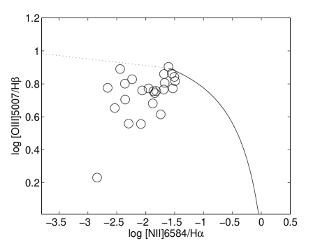
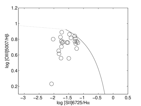
Figure 2: BPT diagrams including all the objects (open circles) described in Table 1. The black solid line is taken by Kauffmann et al (2003). The black dotted line is a rough continuation of Kauffmann line towards very low [NII]/H${\alpha}$  and [SII]/H${\alpha}$  line ratios.

Our galaxy sample (Table 1) is shown in the BPT diagrams (Fig. 2). The objects are located in the region of very low [NII]/H${\alpha}$  (left panel) and relatively low [SII]/H${\alpha}$  (right panel) beyond the lower limit of the observed line ratios e.g. for AGN, starburst and HII region galaxies (solid line). They may indicate low N/H and S/H relative abundances and/or matter-bounded emitting clouds such that a large part of the recombination zone is excluded. J0811+4730 corresponds to the lowest [OIII]5007/H${\beta}$  and to the lowest O/H.

BTP diagrams (Kauffmann 2003, Kewley et al 2001) for the [OIII]5007/H${\beta}$  and [NII]6583/H${\alpha}$  line ratios are generally adopted by the author community in order to identify the galaxy type in terms of the radiation source. However, extreme physical conditions and relative abundances far from solar, in particular for O/H and N/H, may shift the observed [OIII]/H${\beta}$  and [NII]/H${\alpha}$  line ratios throughout the BTP diagram towards sectors which were assigned to different galaxy types. For example, a low N/H relative abundance may shift the observed [NII]/H${\alpha}$  line ratio emitted from a AGN towards the SB galaxy domain although other features of the same object are characteristic of an AGN. These diagrams provide an approximated but rapid information of the gas physical conditions within the emitting clouds. (The line and continuum flux are emitted from the nebula). The [OIII]/H${\beta}$  and [NII]/H${\alpha}$  line ratios alone cannot definitively constrain the models because we deal with two line ratios referring to different elements. [OIII]/H${\beta}$  ratios depend on the effective temperature of the star, on the ionization parameter, on the shock velocity, etc., more than on the O/H relative abundance, whereas the [NII]/H${\alpha}$  ratios depend also strongly on the N/H relative abundances. We cannot determine a priori whether the best fit to the observed [NII]/H${\alpha}$  line ratio could be reached by changing one or more input parameters representing the physical conditions (see Appendix A) or by modifying the N/H relative abundance. N⁺ and H⁺ ions as well as O⁺ and H⁺ are correlated by charge exchange reactions, therefore [NII]/H${\beta}$  and [OII]/H${\beta}$  have a similar trend throughout a cloud. When [OIII]/H${\beta}$  (and [OII]/H${\beta}$) are well reproduced by modelling and [NII]/H${\beta}$  is less fitted by solar N/H the N/H relative abundances can be calculated directly from ([NII]/H${\beta}$)_obs = ([NII]/H${\beta}$)_calc (N/H)/(N/H)_⊙, where (N/H)_⊙ is the solar N/H relative abundance. In fact, N is not a strong coolant.

3.2 Detailed modelling results

Our modelling method consists in trying to reproduce all the line ratios reported by the observations in a single spectrum by a particular model characterised by a set of physical parameters and element abundances (see Appendix A for a detailed presentation of the model) which are briefly described in the following. The shock velocity $\rm V_{s}$, the atomic preshock density $\rm n_{0}$ and the preshock magnetic field $\rm B_{0}$ define the hydrodynamical field. The primary radiation from the stars which is represented by the effective star temperature $\rm T_{*}$ and the ionization parameter $U$ affects the surrounding gas. This region is considered as a sequence of plane-parallel slabs. The geometrical thickness $D$ of the clouds is also an input parameter. The fractional abundances of the ions are calculated resolving the ionization equations for each element (H, He, C, N, O, Ne, Mg, Si, S, Ar, Cl, Fe) in each ionization level. The calculated line ratios, integrated throughout the cloud geometrical width, are compared with the observed ones. The calculation process is repeated changing the input parameters until the observed data are reproduced by the model results, at maximum within 10-20 percent for the strong lines and 50 percent for the weak ones. A grid of models is built for each spectrum in order to select the best fit to the data. The observed spectra which strongly constrain the models are those showing MgII2798+, [OII]3727+, [NeIII]3686, [OIII]4363, HeI4471, HeII4686, [OIII]5007+, HeI5876, [OI]6300+, [SIII]6312, [NII]6548+, [SII]6717, [SII]6731, [ArIII]7136, etc (the + indicated that the doublet is considered) and the Balmer lines H${\beta}$, H${\alpha}$  and H${\gamma}$. The higher the number of lines referring to different elements in different ionization levels, the higher is the number of models considered in each grid. Our aim is to find out which lines are the most critical ones trying to fit a rich spectrum by a single-cloud model. When the required precision is not reached, a pluri-cloud model is adopted (e.g. Fonseca-Faria et al 2021). which yields a more detailed picture of the physical parameter and element abundance distribution throughout the observed region.

To chose the grid models we should consider that in a hydrodynamical regime of gas outflowing from the starburst (e.g. Yu et al 2021) the shock front is on the external edge of the clouds. The gas throughout the shock front and downstream is heated to high temperatures depending on the shock velocity and it is compressed, increasing the cooling rate. Consequently, through the emitting cloud, the regions of gas emitting the different lines have different sizes. The internal edge of the clouds - facing the radiation source - is heated by the photoionization flux from the stars to temperatures of $\sim$ 2-3 $\times 10^{4}$K which correspond to strong lines from intermediate ionization levels. Therefore, strong lines from high ionization levels can be predicted in a single spectrum together with lines from intermediate levels and recombination lines due to the rapid temperature drop downstream. Each line intensity is integrated through the cloud following the profile of $\rm T_{e}$ and $\rm n_{e}$ . Consequently, the spectra can show unexpected line ratios. In the following we will identify the galaxies only by their right ascension for sake of table formatting.

The observed line ratios to H${\beta}$  of the selected galaxies are presented in Tables 1, 2, 5, 7, 9 and 10 and the calculated ones which approximatively reproduce the observations are shown in the line (or column as in Table 10) next to the data for each object (models mis1a-mis9a, mis1b-mis9b, miss1-miss6, mG1-mG4, mpa-mpb, misss1-misss2, and B1m-B7m). For a few galaxies we present different models for the same observed spectrum in order to give a hint on the selection criteria adopted in the present work. The physical parameter and element abundance sets which characterize the models are shown in Tables 3, 4, 6, 8, 9 and 10. The relative abundances of the most significant elements to H calculated in the present work are compared with the results obtained by the other methods in the bottom of the tables. The results obtained by the detailed modelling method are selected by a compromise between calculation precision and observed uncertainties. Moreover, a further approximation cannot be avoided considering that the observations cover an entire galaxy including gas in different physical conditions. The physical picture is not homogeneous throughout the galaxies. Therefore, the observed data for each object cannot be always satisfactorily fitted with high precision by the results of a single-cloud model which represents a specific physical situation.

Table 2: Comparison of observations for I20 survey and J1234 (I19b) galaxy with model results. H${\beta}$=1

	[OII]	[NeIII]	[OIII]	HeI	HeII	[OIII]	HeI	[OI]	[SIII]	[NII]	[SII]	[SII]	[ArIII]
	3727+	3868	4363	4471	4686	5007+	5876	6363	6213	6584	6717	6731	7136
J0007	0.24	0.57	0.197	0.035	0.013	10.35	0.107	0.005	0.009	0.01	0.029	0.022	0.037
mis1a	0.23	0.78	0.10	0.047	0.026	11.	0.127	3e-5	0.05	0.011	0.018	0.015	0.09
mis1b	0.20	1.2	0.14	0.040	0.04	11.88	0.13	2e-4	0.05	0.02	0.017	0.029	0.09
J0159	0.184	0.58	0.22	0.042	0.014	8.44	0.11	0.005	0.007	0.012	0.013	0.013	0.02
mis2a	0.20	0.5	0.19	0.002	0.07	8.37	0.005	4.e-5	0.04	0.013	0.015	0.014	0.02
mis2b	0.21	0.4	0.04	0.03	0.026	8.3	0.09	2.e-5	0.02	0.011	0.009	0.009	0.02
J0820	0.28	0.5	0.21	0.03	0.0	7.6	0.076	0.0	0.0	0.0	0.03	0.014	0.032
mis3a	0.24	0.58	0.17	0.012	0.07	7.69	0.03	2e-5	0.039	0.01	0.007	0.006	0.03
mis3b	0.25	0.4	0.05	0.03	0.03	7.2	0.086	4e-5	0.016	0.019	0.012	0.011	0.025
J0926	0.23	0.48	0.198	0.04	0.009	8.97	0.12	0.0	0.009	0.016	0.021	0.025	0.027
mis4a	0.21	0.70	0.23	0.001	0.09	8.6	0.003	4.e-5	0.052	0.01	0.019	0.016	0.028
mis4b	0.18	0.70	0.10	0.05	0.011	9.67	0.13	4.e-6	0.03	0.013	0.005	0.003	0.03
J1032	0.25	0.48	0.198	0.04	0.012	8.15	0.12	0.009	0.011	0.02	0.026	0.025	0.03
mis5a	0.3	0.4	0.24	0.03	0.047	8.0	0.01	5.4e-5	0.034	0.01	0.012	0.01	0.24
mis5b	0.23	0.4	0.06	0.05	0.011	8.0	0.14	1.4e-5	0.03	0.012	0.009	0.008	0.03
J1205	0.20	0.28	0.133	0.043	0.038	5.49	0.12	0.015	0.006	0.05	0.011	0.03	0.018
mis6a	0.3	0.26	0.12	0.069	0.05	5.8	0.18	4e-5	0.044	0.042	0.011	0.01	0.05
J1242	0.20	0.3	0.196	0.046	0.022	6.76	0.093	0.0006	0.007	0.012	0.024	0.025	0.023
mis7a	0.182	0.4	0.22	0.002	0.07	6.8	0.005	3.e-5	0.04	0.011	0.012	0.010	0.018
mis7b	0.18	0.3	0.043	0.049	0.026	6.8	0.14	1.e-5	0.02	0.011	0.008	0.007	0.02
J1355	0.22	0.54	0.21	0.03	0.027	7.96	0.087	0.009	0.012	0.006	0.023	0.026	0.026
mis8a	0.24	0.58	0.17	0.012	0.07	7.69	0.03	2e-5	0.039	0.01	0.007	0.006	0.03
mis8b	0.20	0.5	0.04	0.05	0.022	7.65	0.14	2e-5	0.02	0.009	0.008	0.008	0.026
J1234	0.127	0.128	0.077	0.038	0.024	2.7	0.1	-	-	-	-	-
mis9a	0.12	0.15	0.06	0.036	0.026	4.55	0.1	-	-	-	-	-	-
mis9b	0.1	0.11	0.04	0.067	0.02	2.9	0.2	-	-	-	-	-	-

Table 3: Models adopted in Table 2

	mis1a	mis2a	mis3a	mis4a	mis5a	mis6	mis7a	mis8a	mis9a
$\rm V_{s}$($\rm km\,s^{-1}$)	100	150	100	100	100	100	100	100	100
$\rm n_{0}$ ($\rm cm^{-3}$)	50	63	52	65	62	90	64	52	150
$D$ (0.01pc)	87	0.7	1.4	0.8	0.9	0.5	0.8	1.4	0.5
$\rm T_{*}$ (104K)	6.6	7.6	5.0	9.5	6.2	4.5	7.	5.0	4.0
$U$ -	0.05	0.06	0.095	0.03	0.05	0.09	0.06	0.095	0.3
N/H calc (1)	0.1	0.2	0.12	0.1	0.1	0.3	0.2	0.12	0.1
N/H (1,2)	0.02	0.017	-	0.024	0.023	0.048	0.011	0.0063	-
O/H calc (1)	1.6	2.7	1.8	2.0	2.6	1.7	2.5	1.8	1.7
O/H (1,2)	0.654	0.366	0.308	0.48	0.39	0.277	0.268	0.359	0.2
Ne/H calc(1)	0.4	0.4	0.4	0.4	0.4	0.4	0.4	0.4	0.4
Ne/H (1,2)	0.11	0.071	0.056	0.074	0.066	0.040	0.054	0.068	0.0139
S/H calc (1)	0.2	0.3	0.25	0.2	0.2	0.2	0.3	0.25	0.01
S/H (1,2)	0.0144	0.0057	-	0.0094	0.007	0.0047	0.0052	0.0081	-
Ar/H calc(1)	0.023	0.01	0.023	0.01	0.01	0.023	0.01	0.023	0.01
Ar/H (1,2)	0.00316	0.00114	0.00134	0.0018	0.00157	0.00087	0.001	0.00128	-
He/H calc	0.1	0.01	0.03	0.01	0.01	0.1	0.018	0.03	0.1

¹ in units of 10^-4; ² evaluated by I20 for the first 8 galaxies and by I19b for J1234.

Table 4: Alternative models adopted in Table 2

	mis1b	mis2b	mis3b	mis4b	mis5b	mis6	mis7b	mis8b	mis9b
$\rm V_{s}$($\rm km\,s^{-1}$)	120	100	100	80	80	100	100	100	70
$\rm n_{0}$ ($\rm cm^{-3}$)	300	90	70	50	80	90	50	80	180
$D$ (0.01pc)	7	8	6.67	96.7	16.67	0.5	20	10	0.27
$\rm T_{*}$ (104K)	7.9	5.5	5.5	5.1	4.8	4.5	5.3	5.3	3.6
$U$ -	0.13	0.07	0.05	0.08	0.08	0.09	0.07	0.08	0.4
N/H calc (1)	0.1	0.13	0.2	0.1	0.1	0.3	0.1	0.1	0.1
N/H (1,2)	0.02	0.017	-	0.024	0.023	0.048	0.011	0.0063	-
O/H calc (1)	1.3	5.0	5.7	1.4	2.6	1.7	2.4	4.3	1.2
O/H (1,2)	0.654	0.366	0.308	0.48	0.39	0.277	0.268	0.359	0.11
Ne/H calc(1)	0.4	0.4	0.4	0.4	1.0	0.4	0.7	0.8	0.4
Ne/H (3,2)	0.11	0.071	0.056	0.074	0.3	0.040	0.054	0.068	0.0139
S/H calc (1)	0.1	0.3	0.25	0.2	0.3	0.2	0.3	0.25	0.01
S/H (1,2)	0.0144	0.0057	-	0.0094	0.0074	0.0047	0.0052	0.0081	-
Ar/H calc(1)	0.01	0.007	0.023	0.0073	0.007	0.023	0.007	0.0073	0.01
Ar/H (1,2)	0.00316	0.00114	0.00134	0.0018	0.00157	0.00087	0.001	0.00128	-
He/H calc	0.1	0.1	0.08	0.1	0.1	0.1	0.1	0.08	0.1

¹ in units of 10^-4; ² evaluated by I20 for the first 8 galaxies and by I19b for J1234.

3.2.1 I20 survey

The observed (reddening corrected) line ratios from the I20 survey are shown in Table 1 (Balmer lines) and in Table 2 (other lines). The observations by the Cosmic Origins Spectrograph onboard the Hubble Space Telescope were focused on star-forming galaxies at z = 0.028-0.0065 with low oxygen abundances and extremely high emission-line ratios [OIII]5007/[OII]3727 $\sim$ 22-39. Characteristic of this survey are the simultaneous low [OII]3727+/H${\beta}$  and high [OIII]5007+/H${\beta}$. Generally, in the spectra shown by SFG surveys in the local universe the [OIII]/[OII] line ratios reach values of $\sim$6 e.g. for the Berg et al (2012) survey of galaxies at z $\leq$ 0.023, while for the Marino et al (2013) Califa HII complex at 0.005$<$z$<$0.03 [OIII]5007+/[OII]3727+ is $\leq$ 1 (see also Contini 2017 and references therein). [OII]3727+/H${\beta}$  in a few cases shows values similar to or even lower than [OIII]4363/H${\beta}$. We consider that the relatively large errors as high as 50 percent which are allowed in the fit of the weak line ratios to H${\beta}$  can be applied to [OII]3727+/H${\beta}$  because in the present spectra they are abnormally low (Table 2). The observed [OIII]5007+/[OII]3727+ line ratios range between 45.8 for J0159 and 27.45 for J1205 and the HeII4686/H${\beta}$  between 0.09 and 0.038. [OIII] 4363/H${\beta}$  covers a small range (0.196-0.22) except for J1205 with [OIII]4363/H${\beta}$=0.13. [OIII]4363 can be blended with H${\gamma}$. The [OIII]5007+/[OIII]4363 ratios (hereafter R_[OIII]) range from 34.5 for J1242+4851 to 52.5 for J0007+0226. Such low R_[OIII] values indicate that the [OIII] lines, in particular [OIII]4363, are emitted from a relatively hot gas when the effect of the shock dominates on photoionization (Aldrovandi & Contini 1985). All the line ratios to H${\beta}$  are low compared to [OIII]5007+/H${\beta}$  by a factor $\geq$ 5 in contrast to the spectra generally presented for starburst and SFG at low redshift. We have added in Tables 2, 3 and 4 the galaxy J1234+3901 (I19b) even if it is located at a higher redshift (z=0.13297) because the HeII line has been observed constraining the model as for the other SFG of the I20 sample.

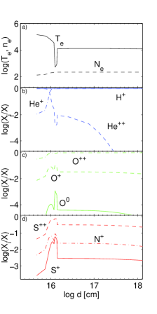
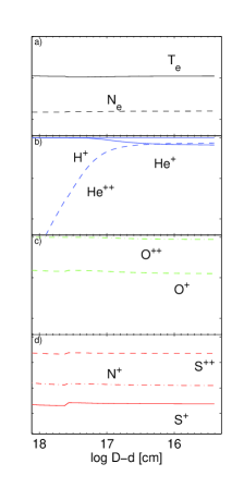
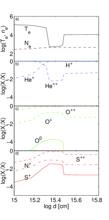
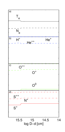
Figure 3: The profiles of the electron temperature the electron density (top panels) and of the fractional abundances of the H, He, N, O and S different level ions throughout the emitting cloud. Top diagrams: J007+0226; bottom diagrams: J1205+4551. The clouds are divided in two halves. In the left panel the shock front is on the left and the X-axis scale is logarithmic. In the right panel the right edge is reached by the flux from the starburst. The X-axis scale is logarithmic in reverse, in order to have the same detailed view of the cloud edges (the shock-dominated and the radiation-dominated one).

To better understand the modelling results we show in Fig. 3 diagrams the profiles of $\rm T_{e}$ , $\rm N_{e}$ and of the fractional abundance of the most significant ions throughout the clouds corresponding to J0007 (top, model mis1a) and J1205 (bottom, model mis6a). For each galaxy the emitting cloud is divided into two equal and antisymmetrical parts in order to see the results with relatively high precision at the two opposite edges. When the cloud propagates outwards from the starburst the shock front is on one edge (at the left of the left panels in Fig. 3) while the opposite edge (at the right of the right panels) is reached by the photoionization flux from the starburst. Using composite models the gas can reach relatively high temperatures $\rm T_{e}$ near the shock front depending on the shock velocity ($T\sim$1.5$\times 10^{5}$ ($\rm V_{s}$/100 $\rm km\,s^{-1}$)²). Radiation from the stars heats the opposite edge to no more than 2-3$\times$10⁴K. The $\rm T_{e}$ profile throughout the emitting clouds is not straightforward, decreasing towards the cloud centre following the cooling rate. Fig. 3 shows that the high temperature downstream close to the shock front would correspond to a not negligible O³⁺/O fractional abundance. The gas recombines and O⁺⁺/O increases, while He⁺⁺/He decreases. He⁺⁺/He from the edge of J0007 clouds reached by radiation decreases due to radiation transfer. $\rm T_{e}$ is maintained at $\leq$10⁴K by secondary radiation. The effective starburst temperature $\rm T_{*}$ affects the black-body radiation flux and, combined with the ionization parameter $U$, they yield different [OIII]5007+/[OII]3727+ line ratios. HeII line intensity depends strongly on the photoionization flux from the radiation source. Therefore, for J0007 this line comes in particular from the radiation dominated zone (right panel), while for J1205 the only zone of gas with a temperature high enough to emit a strong HeII line is downstream, close to the shock front (left panel) because $\rm T_{*}$ is relatively low.

The J0007 spectrum is fitted satisfactorily enough by model mis1a. The disagreements between calculated and observed [OIII]4363/H${\beta}$  and HeII4686/H${\beta}$  ratios reach a factor $\leq$ 2, while HeI4471/H${\beta}$  and HeI5876/H${\beta}$  are well reproduced. The results indicate that for J0007 Ar/H should be reduced by a factor of $\geq$2. In the same spectrum the [OI]/H${\beta}$  and [SIII]/H${\beta}$  are underestimated and overestimated by large factors, respectively. The [SII]/H${\beta}$  line ratios are both underestimated. They are calculated with solar S/H relative abundances. Therefore, the sulphur line fit cannot improve by increasing S/H. As it was explained by Congiu et al (2017), [OI] refers to a recombined oxygen and [SII] depend on S⁺ which has a ionization potential lower than that of H⁺. They suggest that [OI] and [SII] lines are contaminated by the ISM which is in the same characteristic physical conditions. The J0007 spectrum shows the maximum observed [OIII]5007+/[OII]3727+ line ratio relatively to the objects in the I20 survey, but the other line ratios are similar. We have tried to reproduce the J0007 spectrum with another model (mis1b) described in Table 4 with a different approach i.e. to reduce the successful fit of some strong line ratios to H${\beta}$  and to improve that of the weak ones e.g. [OIII]4363/H${\beta}$. The calculated [OIII]4363/H${\beta}$  line ratio is lower than observed by a factor of $\sim$1.4, while the calculated HeII/H${\beta}$  is higher than observed by a factor of $\sim$ 3. Moreover, the [SII]6717/6731 line ratio is $<$1 while the observed one is $>$ 1 for model mis1b due to the high preshock density. The S/H ratio adopted for model mis1b is lower than solar indicating that S is included into dust grains. The geometrical thickness $D$ (Table 3) calculated by model mis1a exceeds $D$ resulting for all the other I20 survey galaxies by a factor of $\sim$ 10, while $D$ for model mis1b is similar to that calculated for the other I20 survey objects. We select model mis1a to represent J0007 spectrum because [OIII]5007+/H${\beta}$  and HeII/H${\beta}$  are reproduced with smaller errors. The J0007 spectrum analysis however suggests that it is unrealistic to reproduce the spectrum of each galaxy by a single model. Therefore in the following we will present two sets of models (mis1a-mis9a) and (mis1b-mis9b) for I20 survey galaxies and for J1234 in Tables 3 and 4, respectively. Both sets satisfactorily reproduce the [OIII]5007+/H${\beta}$, [OII]3727+/H${\beta}$  and [NII]/H${\beta}$  ratios. Models mis1a-mis5a and mis7a-mis8a better fit [OIII]4363/H${\beta}$, while mis2b-mis5b and mis7b-mis8b reproduce satisfactorily HeII/H${\beta}$. The two sets of models show extreme [OIII]4363/H${\beta}$  and HeII/H${\beta}$  which indicate that averaged models may produce a better fit to the observed weak line ratios. J1205 spectrum is well reproduced by one model because mis6a is identical to mis6b. Moreover, [OIII]4363/H${\beta}$  and HeII/H${\beta}$  line ratios in J1234 are well reproduced by both mis9a mis9b, but mis9a should be dropped because [OIII]5007+/H${\beta}$=4.55 is unacceptably high.

Table 3 shows that the shock velocities are $\geq$100 $\rm km\,s^{-1}$for this galaxy sample, while Table 4 indicates $\rm V_{s}$$\leq$100 $\rm km\,s^{-1}$for a few objects. The preshock densities are all $\leq$ 100 $\rm cm^{-3}$, except for model mis1b with $\rm n_{0}$=300 $\rm cm^{-3}$, which although yielding a better fit of the [OIII]4363/Hb  line ratio, it reproduces the other ones with larger errors. For mis9b $\rm n_{0}$=180 $\rm cm^{-3}$ leads to a good fit of the J1234 spectrum. The star effective temperatures for the I20 sample range between 50000K and 95000K, except for mis5a and mis6a with $\rm T_{*}$ = 48000K and 45000K, respectively. The ionization parameter $U$ is in the norm for SF galaxies at these redshift (e.g. Berg et al 2012). The geometrical thickness of the emitting clouds ranges between 0.005 pc for J1205 and 0.97pc for J0926. This large $D$ would imply a large region of neutral gas within the cloud yielding a high [OI]6360/H${\beta}$  ratio. For all the models the calculated [OI]/H${\beta}$  is nearly null. Considering that the [SIII]6312 line lies within the [OI]6300,6363 doublet, that these lines are blended for $\rm V_{s}$$\geq$100$\rm km\,s^{-1}$, that [SIII]/H${\beta}$  calculated by the models (Table 3) are all exceeding the data and that the observed [OI] lines are contaminated by the ISM component, such a low [OI]/H${\beta}$  is acceptable. The sum of [OI] and [SIII] lines should be considered. With regards to the element relative abundances (Tables 3 and 4), we obtain lower than solar O/H by factors of $\sim$1.2-5 ([O/H]_⊙=6.6$\times$10^-4), N/H by factors between 3 and 10 ([N/H]_⊙=10^-4) and Ar/H by factors 2-6.5 ([Ar/H]_⊙=4.6$\times$10^-6). On the other hand S/H is about solar ([S/H]_⊙=2$\times$10^-5). This result strengthens our suggestion that the observed [SII] lines have a strong ISM contribution.

An unusual result for the I20 sample galaxies consists in the He/H ([He/H]_⊙=0.1) adopted in the mis2a-mis5a and mis7a-mis8a models which are lower than solar by different factors. They were used to better reproduce the HeII/H${\beta}$  line ratios. However, they reduce the HeI5876/H${\beta}$  calculated line ratios in some objects. The HeI5876/H${\beta}$  observed values range between $\leq$0.1 and $\leq$0.15 in Table 2 objects and in most of the observed spectra from different types of galaxies at different redshift. In fact H${\beta}$  and HeI 5876 are both recombination lines and they behave similarly throughout large regions of the clouds at temperatures $\leq$10⁴K (Fig. 3) even if matter-bounded. The models presented in Table 4 better reproduce the HeII/H${\beta}$  data adopting He/H near solar for most of them. The [OIII]4363/H${\beta}$  line ratios are generally underpredicted by these models. Even considering that H${\gamma}$4340 and [OIII]4363 lines could be partly blended at $\rm V_{s}$$\sim$ 100 $\rm km\,s^{-1}$, this does not resolve the problem because H${\gamma}$/H${\beta}$  are nearly constant (Table 1) and show suitable values and [OIII]4363/H${\beta}$  ratios show similar values for most of the I20 spectra.

Concluding, we have found by fitting the [OIII] 5007/H${\beta}$, [OIII]4363/H${\beta}$, [OII]/H${\beta}$, [NII]/H${\beta}$  and [SII]/H${\beta}$  line ratios and selecting the physical parameters and the relative abundances, that the HeII/H${\beta}$  line ratios constrain the models by the geometrical thickness of the cloud and by the He/H abundance ratio. Table 2 shows that both [OIII]4363/H${\beta}$  and HeII4686/H${\beta}$  line ratios depend on $D$, therefore to better reproduce the observed spectra pluri-cloud models seem more realistic. The large range of the calculated different geometrical thickness of the clouds is in agreement with cloud fragmentation due to turbulence created by the shocks at the shockfront. Recall that the observations cover regions with different physical and chemical conditions. Therefore a pluri-cloud model should be used to reproduce each spectrum. Here, we try to reduce a pluri-cloud ensemble to a minimum of two clouds which both show a good fit of calculated to observed strong line ratios (to H${\beta}$) and of a few significant weak ones (e.g. [OIII]4363/H${\beta}$  or HeII4686/H${\beta}$). The worst fit is still acceptable due to the observation error and to the uncertainty of the data used in the calculations. Therefore, an average of these two models represents the best option.

3.2.2 I18b survey

Table 5: Comparison of observations for I18b survey, J0811 (I18a) and HS0837 (P04) galaxies with model results. H${\beta}$=1

	MgII	[OII]	[NeIII	[OIII]	HeI	HeII	[OIII]	HeI	[OI]	[SIII]	[NII]	[SII]	[SII]	[ArIII]
	2796+	3727+	3868	4363	4471	4686	5007+	5876	6360	6312	6584	6717	6731	7136
J0901	-	0.815	0.46	0.076	0.039	-	8.75	0.096	0.032	-	0.093	0.055	0.054	-
miss1	0.21	0.81	0.46	0.11	0.032	-	8.8	0.091	3e-4	0.046	0.088	0.052	0.046	-
J1011	-	0.297	0.497	0.146	0.028	-	10.68	0.117	0.022	0.043	0.07	-	-	-
miss2	0.08	0.28	0.6	0.16	0.024	-	10.78	0.07	4e-5	0.024	0.073	-	-	-
J1243	-	0.537	0.49	0.155	0.031	-	9.65	-	-	-	0.058	-	-	-
miss3	0.15	0.57	0.53	0.147	0.035	-	9.66	0.1	1.e-4	0.04	0.06	0.026	0.023	-
J1248	0.17	0.49	0.46	0.177	0.042	-	7.77	0.10	0.022	-	0.057	0.026	0.031	0.037
miss4	0.11	0.49	0.12	0.14	0.04	-	7.76	0.11	3e-5	0.038	0.046	0.02	0.02	0.046
J1256	0.26	0.443	0.55	0.164	0.04	-	9.73	0.11	-	-	0.079	0.038	0.056	-
miss5	0.26	0.44	0.54	0.17	0.03	-	9.97	0.07	-	-	0.05	0.038	0.033	-
J0811	-	0.167	0.13	0.063	0.036	0.023	2.27	0.095	-	0.004	0.0072	0.014	0.0123	0.01
miss6	-	0.141	0.12	0.04	0.07	0.008	2.66	0.23	3.e-6	0.047	0.007	0.0046	0.04	0.02
HS0837	-	0.41	0.42	0.166	0.037	0.019	7.674	0.13	0.024	0.014	0.024	0.041	0.035	0.034
mpa	-	0.43	0.40	0.15	0.007	0.06	7.76	0.02	1.3e-4	0.07	0.03	0.04	0.043	0.040
mpb	-	0.43	0.35	0.042	0.039	0.016	8.0	0.11	1.0e-4	0.054	0.029	0.037	0.037	0.039

Table 6: Models adopted in Table 5

	miss1	miss2	miss3	miss4	miss5	miss6	mpa	mpb
$\rm V_{s}$($\rm km\,s^{-1}$)	100	100	100	100	100	70	130	100
$\rm n_{0}$ ($\rm cm^{-3}$)	64	63	64	63	95	190	100	100
$D$ (0.01pc)	1.96	1.33	1.43	1.33	0.6	0.2	0.4	6.67
$\rm T_{*}$ (104K)	6.2	6.3	6.2	5.2	7.0	3.4	6.5	5.5
$U$ -	0.016	0.055	0.025	0.044	0.03	0.3	0.035	0.04
N/H calc (1)	0.17	0.55	0.2	0.2	0.3	0.1	0.1	0.1
N/H (1,2)	0.087	0.14	0.056	0.035	0.072	0.0028	0.067	0.067
O/H calc (1)	2.7	2.7	2.6	2.6	2.8	1.0	2.5	2.8
O/H (1,2)	1.44	0.98	0.77	0.44	0.74	0.095	0.44	0.44
Ne/H calc(1)	0.3	0.3	0.3	0.3	0.5	0.1	0.3	0.3
Ne/H (1,2)	0.25	0.14	0.12	0.07	0.012	0.015	0.067	0.067
S/H calc (1)	0.16	0.16	0.16	0.2	0.3	0.3	0.24	0.28
S/H (1,2)	-	-	-	-	-	0.002	0.017	0.017
Mg/H calc (1)	0.16	0.16	0.16	0.3	0.3	0.3	0.3	0.3
Mg/H (1,2)	-	-	-	0.014	0.04	-	-	-
Ar/H calc (1)	0.007	0.007	0.007	0.007	0.007	0.007	0.005	0.005
Ar/H (1,2)	-	-	-	0.0016	-	2.66e-4	0.0023	0.0023
He/H calc (1)	0.07	0.08	0.08	0.08	0.08	0.1	0.02	0.08

¹ in units of 10^-4; ² relative abundances are evaluated by I18b for the first 5 galaxies presented in Table 5, by I18a for J0811 and by P04 for HS0837.

Table 7: Comparison of observations for G20 survey galaxies with model results. H${\beta}$=1

	MgII	[OII]	[NeIII]	[OIII]	HeI	HeII	[ArIV]	[OIII]	HeI	[OI]	[SIII]	[NII]	[SII]	[SII]	[ArIII]	[OII]	[SIII]
	2789	3727+	3868	4363	4471	4686	4713	5007+	5876	6360+	6213	6584+	6717	6731	7136	7320	9304
J0901	0.225	0.9	0.55	0.11	0.04	0.009	0.01	9.27	0.11	0.045	0.013	0.15	0.077	0.069	0.059	0.034	0.24
mG1	0.24	0.92	0.47	0.07	0.034	0.02	0.02	9.45	0.10	5e-4	0.05	0.12	0.073	0.064	0.050	0.24	0.2
J0925	0.215	1.1	0.49	0.072	0.04	0.011	0.01	7.9	0.11	0.04	0.013	0.14	0.09	0.078	0.06	0.038	0.28
mG2	0.20	1.19	0.45	0.06	0.04	0.019	0.01	8.28	0.11	1e-3	0.06	0.16	0.10	0.09	0.05	0.032	1.0
J1154	0.19	0.49	0.52	0.13	0.039	0.02	0.05	7.62	0.11	0.03	0.011	0.067	0.046	0.036	0.035	-	0.043
mG3a	0.2	0.54	0.5	0.11	0.03	0.19	0.04	7.68	0.08	2e-4	0.067	0.07	0.05	0.04	0.05	0.023	0.9
mG3b	0.25	0.53	0.6	0.072	0.037	0.017	0.02	7.58	0.1	3e-4	0.06	0.08	0.06	0.05	0.03	0.016	0.7
J1442	0.38	0.94	0.73	0.106	0.035	0.01	0.018	8.53	0.1	0.04	0.013	0.10	0.087	0.065	0.05	0.03	0.38
mG4a	0.38	0.95	0.9	0.106	0.022	0.07	0.01	8.32	0.06	5e-4	0.05	0.11	0.074	0.065	0.04	0.032	0.9
mG4b	0.36	1.0	0.6	0.063	0.023	0.03	0.007	8.59	0.07	7e-4	0.056	0.13	0.095	0.083	0.05	0.028	0.9

Table 8: Models adopted in Table 7

	mG1	mG2	mG3a	mG3b	mG4a	mG4b
$\rm V_{s}$($\rm km\,s^{-1}$)	100	100	80	80	100	100
$\rm n_{0}$ ($\rm cm^{-3}$)	64	64	68	60	64	64
$D$ (0.01pc)	10	8.33	1.53	46.6	2.07	6.66
$\rm T_{*}$ (104K)	6.2	6.0	6.7	6.4	6.4	6.4
$U$ -	0.016	0.013	0.014	0.019	0.012	0.012
N/H calc (1)	0.18	0.18	0.14	0.12	0.17	0.17
N/H (1,2)	0.088	0.08	0.04	0.04	0.06	0.06
O/H calc (1)	2.7	2.5	1.5	1.5	2.6	2.6
O/H (1,2)	1.11	1.3	0.56	0.56	0.97	0.97
Ne/H calc(1)	0.3	0.3	0.3	0.3	0.6	0.6
Ne/H (1,2)	0.2	0.26	0.09	0.09	0.19	0.19
S/H calc (1)	0.16	0.16	0.16	0.16	0.16	0.16
S/H (1,2)	0.024	0.024	0.01	0.01	0.02	0.02
Ar/H calc(1)	0.007	0.007	0.007	0.007	0.007	0.007
Ar/H (1,2)	0.004	0.004	0.002	0.002	0.0032	0.0032
Mg/H calc (1)	0.16	0.16	0.1	0.1	0.22	0.22
He/H calc	0.07	0.08	0.07	0.07	0.05	0.05

¹ in units of 10^-4; ² evaluated by G20.

I18b presented observations obtained by the Cosmic Origin Spectrograph onboard the Hubble Space Telescope of galaxies within the z range 0.2993-0.4317 and high [OIII]5007+/[OII] 3727+. The comparison of the observed line ratios with the results of calculation by detailed modelling is shown in Table 5. The models are described in Table 6. [OII]/H${\beta}$  ratios for the I18b survey spectra are higher by factors $>$ 2 than for the I20 survey galaxies. The spectra contain the MgII 2796,2803 lines. Table 5 shows that models miss1-miss4 are similar for galaxies J0901, J1011, J1243 and J1248 but for J1256 miss5 shows a different set of parameters. In particular, $\rm T_{*}$ and $\rm n_{0}$ are higher than for the other survey galaxies by a factor $\leq$ 1.5. The element relative abundances to H for all the galaxies are lower than solar, except for S/H that even exceeds the solar value in miss5. In particular, O/H are $\sim$0.4 solar and Ar/H are 0.15 solar. HeII4686 lines were not observed. We constrain the models by an HeII/H${\beta}$  upper limit $<$0.1. The best fit to the observed HeI/H${\beta}$  ratios is obtained by He/H=0.08, slightly lower than solar (0.1). Comparing our results with those derived by I18b, the relative abundances of all the elements are higher by factors $\sim$ 2 - 6 for O/H, 2-4 for N/H, 1.2-5 for Ne/H and for Ar/H by a factor of $\leq$28 for J1354. S/H and He/H were not indicated by I18b.

3.2.3 J1234+3901 (I19b)

We have added to the I20 survey the spectrum of the most metal-poor galaxy J1234+3901 at z=0.133. Tables 2-4 include the modelling of J1234+3901 galaxy spectrum (I19b). Optical spectroscopy of this galaxy in the local Universe was obtained by the LBT/MODS telescope. The J1234+3901 galaxy spectrum and the models are described in the bottom three lines of Table 2 and in the last column of Tables 3 and 4. Model mis9a, which reproduces at most the HeI and HeII line ratios to H${\beta}$, overpredicts [OIII]5007+/H${\beta}$  by 68 percent. The [OIII]5007 line is the strongest one, therefore it requires a more accurate model. Model mis9b satisfactorily reproduces the [OIII]5007+/H${\beta}$  line ratio. It underpredicts [OIII]4363/H${\beta}$  by a factor $<$2 which, however, is within the accepted error, being [OIII] 4363 a weak line. Model mis9b shows relatively high $\rm n_{0}$=180 $\rm cm^{-3}$ and low $\rm V_{s}$=70 $\rm km\,s^{-1}$. The effective temperature of the stars is the lowest for all the sample galaxies (36000K) and the high ionization parameter $U$=0.4 compensates the modelling of the strongest line ratios. N/H and O/H are particularly low, 0.1 solar and 0.18 solar, respectively, while He/H=0.1. Model mis9b is selected because it reproduces all the weak line ratios within a factor of 2 (Table 4). In model mis9b $D$=0.0027 pc is very thin and indeed it leads to more acceptable results. However, changing $D$, all the line ratios change as well and, in particular the good fit of the [OIII]5007+/H${\beta}$  and [OII]3727+/H${\beta}$  calculated to observed line ratios may be lost. We suggest that to improve the modelling of the survey galaxy spectra, the final line ratios should be calculated from the average of single-cloud spectra.

3.2.4 J0811+4730 (I18a)

I18a present a rich observation spectrum of galaxy J0811+4730 at z=0.044 from the Data Release I3 (DRI3) of Sloan Digital Sky Survey (SDSS) LBT/MOD with high signal-to-noise ratios. By the direct $\rm T_{e}$ strong line method they obtain 12+log(O/H)=6.98. I18a explain the low metallicity by infall of poor metallic gas from the galactic halos mixing with the metal rich gas in the central region (Ekta & Chengalur 2010). We have revisited the spectrum by the detailed modelling of the line ratios. The results which appear in Tables 1, 5 and 6 (model miss6) well reproduce the [OII]/H${\beta}$, [OIII]5007+/H${\beta}$, [NeIII]/H${\beta}$  and [NII]/H${\beta}$  ratios, roughly fit [OIII4363/H${\beta}$  and HeI/H${\beta}$  line ratios, but they underpredict HeII/H${\beta}$  by a factor $\leq$ 3. The S lines are even less fitted. Model miss6 shows (Table 6) that although the O/H and N/H calculated results are 0.15 and 0.1 solar, respectively, they are still higher than those evaluated by I18a (0.014 and 0.0028 solar, respectively). Also for this spectrum we suggest that the [OI], [SII] and HeI lines are most probably contaminated by the ISM.

3.2.5 HS0837+4717 (P04)

We report Pustilnik et al (2004) observations which show the results of high S/N long-slit spectroscopy with the Multiple Mirror and the SAO 6-m telescope, optical imaging with the Wise 1-m telescope and the HI observations with the Nancay Radio Telescopes of the very metal deficient (12+log(O/H)=7.64) luminous blue compact galaxy HS0837+4717 at z=0.041950. This galaxy should belong to the galaxy group at z $<$0.2 presented in Table 2, but it is dislocated in Table 5 as well as J0811 for sake of space. By the direct method analysis of the line ratios Pérez-Montero et al. (2011) claim that nitrogen is overabundant. We have obtained an N/H abundance ratio of 10^-5 by the detailed modelling of the observed spectrum, $\sim$1.5 times higher than that evaluated by P04. Table 6 columns 8 and 9 show the models which better reproduce the data. We have found that model mpa better fits the [OIII]4363/H${\beta}$  line ratio while model mpb reproduces HeII 4686/H${\beta}$  and both the HeI/H${\beta}$  lines. We think that mpa and mpb must be averaged because they represent extreme cases in the starburst. We have found that - as for the other samples - the O/H ratios are by a factor $\sim$ 2.5 lower than solar in agreement with the results obtained by fitting I20 and I19a local SF galaxies. N/H= $\sim$10^-5 relative abundance is similar to those calculated for other SF galaxies. Moreover, our results show that in agreement with Pustilnik et al the starburst is young as revealed from the relatively high $\rm T_{*}$ = 62000K.

3.2.6 G20 survey

Using the (Very Large Telescope) VLT/Shooter spectral observations Guseva et al (2020) presented the spectra of five SF galaxies at z$\sim$0.3-0.4 which contain a rich number of lines from different elements in different ionization levels. In Tables 7 we compare the observed line ratios with model results calculated by detailed modelling. The models are described in Table 8. Two galaxies J0901 and J1011 in the G20 survey are included in the I18b survey. We have repeated the J0901 modelling because G20 observations contain more lines e.g. [OII]7320+ and [SIII]9304. J0901 and J0925 spectra are reproduced by single models, mG1 and mG2, respectively. For J1154 and J1442 we show the results of two models calculated by different $D$. The other input parameters are similar. [SIII]9304/H${\beta}$  is well fitted only for J0901. The results confirm that $D$ is the key parameter which can better reproduce the HeII/H${\beta}$  line ratios even if it affects [OIII]4363/H${\beta}$. Comparing the present results for metallicities with those evaluated by G20 Table 8 shows that N/H calculated in this work are by a factor $\geq$1.5-3 higher than those evaluated by G20, O/H by a factor between 2 and 3 higher, Ne/H by a factor 1.5-3, S/H by $\sim$ 8 and Ar/H by a factor of $\sim$ 2 higher. We have found that He/H are between 0.5 and 0.8 solar.

Table 9: Comparison of observations (I19a survey galaxies) with model results. H${\beta}$=1

	[OII]	[OIII]	[OIII]	[NII]	[OII]	$\rm V_{s}$	$\rm n_{0}$	$D$	$\rm T_{*}$	$U$	N/H	O/H
	3727+	4363	5007+	6584	7320	$\rm km\,s^{-1}$	$\rm cm^{-3}$	0.01pc	104K	-	10-4	10-4
J0314	0.494	0.084	3.304	0.113	0.021	-	-	-	-	-	-	0.21
misss1	0.47	0.076	4.4	0.09	0.023	100	100	1.8	5	0.036	0.25	1.8
J1433	0.914	0.078	3.352	0.066	0.04	-	-	-	-	-	-	0.21
misss2	0.97	0.08	3.65	0.05	0.046	100	100	1.6	4.7	0.019	0.1	2.0

¹ obtained by the direct method (I19a)

3.2.7 I19a survey

The lines presented in this survey are only the most significant oxygen ones [OIII]4363, [OIII]5007+ and seldom [OII]3727. However, the spectra contain [OII]7322 which constrains the models. In Table 9 both the comparison of calculated to observed line ratios and the models are shown. We selected from the rich I19a observed survey only two galaxies J0314 at z=0.02741 and J1433 at z=0.02027 which show a set of line ratios adapted to constrain the models. In columns 2-5 of Table 9 the line ratios to H${\beta}$  are shown. The following columns contain the model sets. I19a have selected in their survey only galaxies with 12+log(O/H) $<$ 7.4. They compare the results obtained by different direct methods. By the detailed modelling of the spectra we find O/H= 1.8 -2.0$\times$10^-4 and N/H= 0.25 - 0.1$\times$10^-4 for J0314 and J1433, respectively. I19a calculated O/H=0.2$\times$10^-4 for the two galaxies J0314 and J1433, which corresponds to O/H lower by a factors of 9 and 10 than calculated by detailed modelling. The comparison about the results calculated by the strong line methods and detailed modelling is discussed in the follow.

3.2.8 B16 survey

Berg et al (2016) present UV spectrophotometry of 12 nearby, low metallicity, high ionization HII regions in dwarf galaxies at z=0.003-0.04 obtained by the Cosmic Origins Spectrograph on the Hubble Space telescope. They selected seven galaxies to analyse the O⁺² and C⁺² ions. We try to reproduce the data from the Berg et al (2016) sample by the detailed modelling of both the UV and optical spectra in order to calculate the C/O and C/N relative abundances for local star-forming galaxies. Modelling results are presented in Table 10. B1o-B7o refer to observations and B1m-B7m to model calculations. Our results confirm that the C/H and N/H are lower than solar, yet they are by a factor $>$ 10 higher that those calculated by the strong line method.

Table 10: Comparison of observations (Berg et al 2016) with model results. H${\beta}$=1

J	082555		104457		120122		124159		122622		122436		124827
	B1o	B1m	B2o	B2m	B3o	B3m	B4o	B4m	B5o	B5m	B6o	B6m	B7o	B7m
CIV1548+1550	0.97	0.82	3.59	3.9	-	2	-	-	-	-	-	-	1.22	0.97
HeII1640	0.38	0.41	0.7	0.64	-	0.48	0.55	0.55	-	-	-	-	0.96	0.75
OIII]1660	1.33	0.9	2.34	0.86	1.6	1.56	1.92	0.73	0.01	0.54	1.8	1.3	0.77	1.5
SiIII]1883+1892	2.41	2.3	1.41	-	-	-	2.4	1.36	-	-	1.29	-	-	4.2
CIII]1906	2.63	3.	2.83	2.5	3.89	3.94	2.94	2.8	0.022	0.019	3.38	3.42	2.12	2.04
CIII]1909	3.44	2.	1.12	1.6	1.8	2.6	1.8	1.8	0.010	0.013	2.96	2.24	1.05	1.33
[OII]3727+3729	-	0.12	-	-	-	-	-	-	-	-	0.97	0.9	0.78	0.79
[NeIII]3869+	0.276	0.6	-	-	-	-	-	-	0.48	0.5?	-	-	-	1.35
H${\gamma}$4340	0.476	0.46	0.506	0.46	0.5	0.46	0.49	0.46	0.49	0.46	0.46	0.45	0.47	0.45
[OIII]4363	0.116	0.15	0.146	0.15	0.11	0.14	0.105	0.136	0.116	0.116	0.111	0.21	0.129	0.25
[OIII]5007+4959	4.83	5.2	6.0	6.1	4.8	4.7	6.4	6.17	7.6	8.0	7.4	7.23	7.9	7.88
[NII]6548+6584	0.019	0.01	0.01	0.013	0.023	0.02	0.05	0.02	0.053	0.04	0.059	0.064	0.04	0.048
H${\alpha}$	2.76	2.96	2.75	3.0	2.78	2.96			2.79	2.97	2.79	3.34	2.78	3.26
[SII]6717	0.026	0.005	0.022	0.017	0.052	0.02	0.088	0.015	0.106	0.017	0.087	0.04	0.084	0.058
[SII]6731	0.022	0.004	0.018	0.014	0.037	0.017	0.076	0.014	0.074	0.019	0.066	0.03	0.059	0.048
[OII]7330	0.012	0.007	0.01	0.02	0.015	0.028	0.11	0.02	0.051	0.026	0.028	0.059	0.019	0.05
$\rm V_{s}$($\rm km\,s^{-1}$)	-	50	-	80	-	70	-	80	-	60	-	80	-	70
$\rm n_{0}$ ($\rm cm^{-3}$)	-	80	-	70	-	80	-	90	-	180	-	80	-	90
$D$ (0.01pc)	-	1.08	-	1.1	-	0.33	-	0.67	-	0.43	-	0.6	-	0.53
$U$	-	0.14	-	0.08	-	0.12	-	0.08	-	0.05	-	0.06	-	0.04
$\rm T_{*}$ (104K)	-	4.1	-	4.6	-	4.2	-	4.6	-	4.6	-	4.2	-	5.0
(C/H)1	-	1.3	-	0.08	-	1.8	-	1.1	-	0.03	-	1.7	-	0.36
(C/H)2	-	0.118	-	0.055	-	0.1	-	0.08	-	0.135	-	0.162	-	0.151
(N/H)1	-	0.2	-	0.07	-	0.12	-	0.1	-	0.26	-	0.16	-	0.13
(N/H)2	-	0.012	-	0.01	-	0.013	-	0.021	-	0.013	-	0.023	-	0.023
(O/H)1	-	1.8	-	1.3	-	1.8	-	1.4	-	4.6	-	1.3	-	1.35
(O/H)2	-	0.23	-	0.282	-	0.282	-	0.537	-	0.794	-	0.692	-	0.646
(S/H)1	-	0.3	-	0.3	-	0.3	-	0.3	-	0.3	-	0.3	-	0.3
(S/H)2	-	0.009	-	0.010	-	0.10	-	0.015	-	0.015	-	-	-	-

¹ in 10^-4 units calculated in this paper; ² in 10^-4 units calculated by Berg et al. (2016)

4 Discussion

In previous sections we have tried to reproduce the observed line ratios in the spectra of local galaxies from different surveys. We have selected from each of them the spectra which could lead to the most reliable results i.e. those which present the highest number of significant lines. Nevertheless, when the observed [OIII]4363 and HeII4686 lines were reported in one spectrum, we had some problem in reproducing both of them with a single-cloud model. We have found that the [OIII]4363/H${\beta}$  and HeII4686/H${\beta}$  line ratios strongly depend on the geometrical thickness of the clouds. $D$ ranges between $\sim$0.002pc and $\sim$1pc. With regards to the other parameters, the detailed modelling method yields $\rm V_{s}$$\leq$ 100 $\rm km\,s^{-1}$(in a few cases $\rm V_{s}$$\leq$150 $\rm km\,s^{-1}$), $\rm n_{0}$ $\sim$ 50-100 $\rm cm^{-3}$, $\rm T_{*}$ =34000-95000K, $U$=0.012-0.4, N/H=0.1-0.55$\times$10^-4 and O/H=1.2-2.8 $\times$10^-4. Three objects show O/H= 4.3, 5.1 and 5.7 $\times$10^-4 which are closer to solar. He/H ranges between 0.01 and 0.1, but most of the spectra were reproduced adopting He/H= 0.08 in agreement with the predicted value (see e.g. Morton 1968).

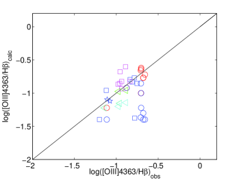
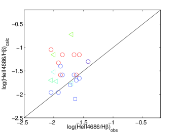
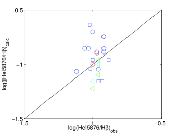
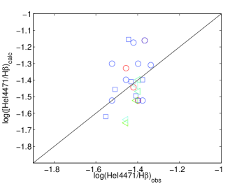
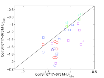
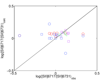
Figure 4: Comparison of model results with the data for I20 survey and J1234 galaxies (red circles: models mis1a-mis9a and blue circles: models mis1b-mis9b), for I18b survey, J0811 and HS0837 (blue squares), for G20 survey (green triangles: models G1, G2, G3a, G4a and cyan triangles: models G3b and G4b), for I19a galaxies (blue stars) and B16 (magenta squares).

4.1 Line ratios

In Fig. 4 model results are compared with the observed line ratios. In the two top left and right diagrams we show the results for the most significant lines, which, however, in SFG they are not always the strongest ones. [OII]3727+/H${\beta}$  can be very low. The observed [NeIII]/H${\beta}$  are less precisely reproduced because [NeIII]3868 may be blended with [NeIII]3967 and with the [[SII]4070,4077 lines which are not negligible at the physical conditions calculated by models which adopt $\rm V_{s}$$\sim$100 $\rm km\,s^{-1}$. About the [NII] line, the error in the observed values is relatively high for low [NII]/H${\beta}$  ($\sim$0.01), reaching 60 percent in the J1355 galaxy. Therefore, the fit in Fig. 4 is less straightforward. The [OIII]4363/H${\beta}$  ratios are underpredicted by the models reported in Table 4 and the HeII4686/H${\beta}$  are overpredicted by models presented in Table 3. Fig. 4 (middle diagrams) suggest that pluri-cloud models averaged on the Table 3 and Table 4 results could improve the fit. The summed [SII]6717+6731 line ratios to H${\beta}$  (Fig. 4, bottom left) are underpredicted by the models even adopting S/H close to solar. Higher S/H relative abundances are not realistic because sulphur is more often trapped into dust grains and depleted from the gaseous phase. We suggest that a large contribution to [SII] comes from ISM regions where dust grains were sputtered by previous strong shock events. The [SII]6717/[SII]6731 (Fig. 4, bottom right) depend on the gas electron density and temperature. The calculated line ratios are nearly constant $\sim$1, while the observations range between $\sim$ 0.3 and 2.2. Even considering the ISM gas inhomogeneous conditions, the extreme low and high observed [SII]6717/6731 indicate $\rm n_{0}$ $>$ 10⁵ $\rm cm^{-3}$ and $<$10 $\rm cm^{-3}$, respectively (Osterbrock 1974), which are not adapted to reproduce the other observed line ratios.

4.2 He lines and He/H relative abundance

In our sample 15 out of 28 spectra include the HeII4686, HeI4471 and HeI5876 lines. In the modelling process we started by [OIII]5007+/H${\beta}$  and [OII]3727+/H${\beta}$. We have found that we could reproduce more precisely [OII]3727+/H${\beta}$  reducing the geometrical thickness of the clouds, however, the fit of HeII4686/H${\beta}$  deteriorated even adopting He/H as low as 0.01 ((He/H)_⊙=0.1). The HeI5876 line is present in the spectra of nearly all types of galaxies with HeI5876/H${\beta}$  ratios in the $\sim$0.1-0.15 range. Fig. 4 diagrams in the row next to the last suggest that the nearly constant observed HeI5876/H${\beta}$  ratios may show a high contamination by the ISM and that they are less affected by radiation from the stars and by radiation from gas collisionally heated by the shocks. The same is valid for HeI4471/H${\beta}$  which is also less affected by the He/H relative abundance than HeI5876/H${\beta}$. Guseva et al (2020) refer to HeII4686 lines as to hard ionizing radiation indicators. They claim that HeII 4686 cannot be emitted from gas photoionized by normal stellar populations with the generally observed temperatures. G20 invoke X-ray from binary stars and shocks as alternatives. Izotov et al (1997) also suggest that the observed HeII 4686/H${\beta}$  cannot be easily reproduced adopting pure photoionization models or $\rm T_{e}$ methods. Shaerer et al (2019) addressing the HeII4686 issue also claim that these lines can be due to X-ray from binary stars. They note that in low metallicity SFG both the empirical data and the theoretical models suggest that high mass X-ray binaries are the main source of nebular HeII emission. In agreement with Guseva et al we have adopted that shocks collisionally heat the emitting gas to high temperatures. We have explained the HeII/H${\beta}$  and the other line ratios by photoionization from the stars coupled to shocks. The sub-solar He/H ratios are calculated consistently with the other results because, heating the gas by the shock, we obtain HeII4686/Hb  higher than observed (see e.g. Table 2).

We suggest that the wind from the starburst region collides with the gaseous clouds throughout the galaxy. Not only the cloud dynamics but also the element composition of the gas within the clouds is affected by the wind from the star atmosphere. In particular, the various He/H abundance ratios found even in nebulae far away from the starburst, trace the WD atmosphere element composition which is conveyed by strong winds. Lauffer et al (2018) explain that WD in the DA spectral class have H-rich atmospheres, DO types show strong HeII lines and T_eff$\sim$ 45000-200000K, while DB types have strong HeI lines and T_eff$\sim$ 11000K-30000K. He/H ratios and other heavy element abundances are connected with the star atmosphere temperatures. Barstow et al (1994) found T_eff$\sim$ 50000K-90000K, in agreement with our results. WD in the present star-forming regions seem of DA type because the HeI lines come most probably from the ISM gas. However they do not exclude contamination by DO and DB types. For most of the models (mis2a-mis8a, Table 3) we could not find any acceptable fit to the observed HeII/H${\beta}$  line ratios by solar He/H. The fit improved reducing the He/H relative abundance by a factor of $\sim$5-10, in agreement with Morton (1968) who reported that ’Miss Underhill believes that He/H for O and B stars lies somehow between 0.05 and 0.01’. This implies a decrease of the HeI 5876/H${\beta}$  line ratio (calculated from the clouds) by a factor $\leq$ 2. However, the fit also improved by using models mis2b-mis8b (Table 4) with a less depleted He/H. For a few galaxies we found He/H = 0.08 in agreement with Morton et al (1968) results which show a minimum of He/H=0.077 in early A- and B-type stars. With regards to the components of close binary systems, Lyubimkov (1995) showed that the low original He/H is maintained throughout the first half of their main sequence evolution, there is no He/H monotonic increase as in the hot isolated stars. The HeII4686 lines are generally weak in galaxies which do not host an AGN. When an AGN is present the spectra show HeII/H${\beta}$  higher than those observed for the I20 survey objects due to the power-law flux from the active nucleus.

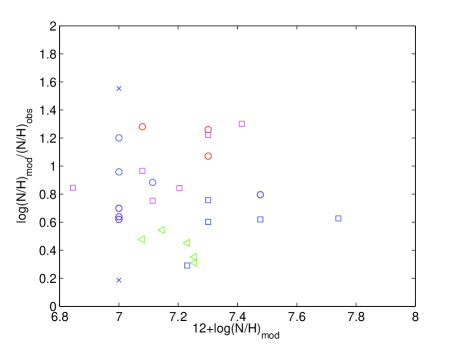
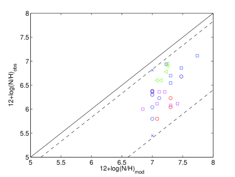
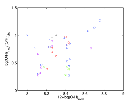
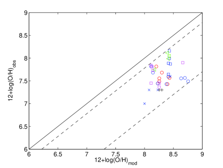
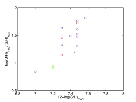
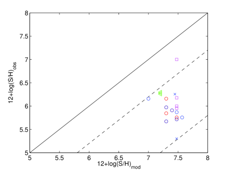
Figure 5: Comparison of relative abundances calculated in this work with those evaluated by the observers using the strong line method: I20 presented in Table 3 (red circles) and in Table 4 (blue circles), I18b presented in Table 6 (blue squares), G20 presented in in Table 8 (green and cyan triangles), I19a presented in Table 9 (black plus) and for galaxies J1234, J0811 and HP0837 presented in Tables 4 and 6 (blue crosses). Top: N/H, middle: O/H and bottom: S/H.

4.3 Relative abundances of the heavy elements

4.3.1 N/H, O/H and S/H

The comparison of the N, O and S metallicities calculated by the detailed modelling and by the direct strong line methods are shown in Fig. 5 (right diagrams). The relative abundances evaluated directly by the observers are all lower than those calculated by detailed modelling. Fig. 5 right diagrams indicate that the relative abundances closest to our model results are given by G20. They also show that O/H calculated by detailed modelling are by factors between 1.6 and 20 higher than those calculated by other methods, N/H by factors $\sim$1.5 and 40 and S/H by factors $\sim$ 6 and 63.

The log((N/H)_mod/(N/H)_obs) versus 12+log(N/H)_mod, log((O/H)_mod/(O/H)_obs) versus 12+log(O/H)_mod and log((S/H)_mod/(S/H)_obs) versus 12+log(S/H)_mod are reported in Fig. 5 left diagrams. They represent the ratios of N/H, O/H and S/H calculated by detailed modelling to those calculatd using the strong line methods by the observers as function of the N/H, O/H and S/H metallicities calculated by detailed method for the sample objects. The trend in Fig. 5 for N/H (left top diagram) is opposite to those of O/H and S/H. N⁺ and H⁺ ions are linked by charge exchange reactions. Accordingly, [NII]/H${\beta}$  depends strongly on N/H. At high N/H, modelling and strong line method results converge because N appears only in the [NII]6584,6548 lines and observation uncertainties are lower. If we omit in the Fig. 5 middle left diagram the three galaxies with a near solar O/H calculated by models mis2b, mis3b and mis8b the trend becomes ambiguous. These models were already criticised because underpredicting [OIII]4363/H${\beta}$  (Table 2). For elements like oxygen which corresponds to a relatively high number of significant lines ([OIII]5007+, [OIII]4363, [OII]3727+, [OI]6300+, etc) in a single optical spectrum, the O/H relative abundances by the strong line methods may lose some important components and underpredict O/H for high O/H. In fact, by detailed modelling the electron temperature and density profiles are calculated throughout the entire clouds, whereas by the strong line methods some regions may be excluded. With regards to S/H, also for S⁺ and H⁺ ions charge exchange reactions are taken into consideration. However, the poor fit of the [SII]/H${\beta}$  ratios calculated by detailed modelling was explained by a strong contribution from the ISM with S/H at their maximum value. Therefore, the trend is opposite to that for N/H.

4.3.2 C/O and N/O relative abundances

A general trend of increasing C/O abundance ratio with O/H and a constant C/N were noticed by Berg et al (2016). We obtain the C/O and N/O ratios by modelling (see Table 10) consistently both the UV and the optical emission lines observed by Berg et al (2016). The C/O ratios calculated in the present paper are reported on top of the log(C/O) versus 12+log(O/H) diagram presented by Berg et al (2016, their fig. 8) in Fig. 6. In particular, they show that log(C/O) rapidly increases at 12+log(O/H)=8. Henry et al (2000) claim that C and N production in the Universe are decoupled and originate from separate sites. Carbon is mainly produced by massive stars (M$>$ 8M_⊙ ), while primary nitrogen production at low O/H is dominated by intermediate-mass stars between 4 and 8 M_⊙ . At 12+log(O/H)$>$8.3 secondary nitrogen becomes prominent. The N/O ratio positively correlates with stellar mass (Perez-Montero et al 2013). Hayden-Pawson et al (2021) report that N/O maintains a constant value log(N/O)$\sim$-1.5 at low metallicities while at higher metallicities the N/O ratio increases rapidly with O/H. Henry et al suggest that the flat N/O is due to low star formation rate in contrast with Izotov & Thuan (1999) who claim that these systems are very young because of their low metallicity. Izotov & Thuan (1998) results for blue compact galaxies show that none of the heavy element-to-oxygen abundance ratios depend on O/H. An investigation of many host galaxy types indicates that secondary nitrogen becomes evident throughout the redshift range (Contini 2017, fig. 7) at z$\leq$0.1. N/O ratios in local HII regions appear at the bottom of the N/O versus z diagram well separated from the AGNs.

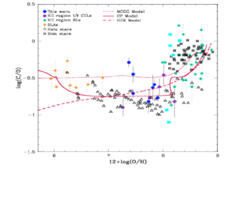
Figure 6: Comparison of C/O relative abundances versus metallicity calculated in this paper (Table 1) (cyan rectangles) with the results reported from Berg et al (2016, their fig. 8)

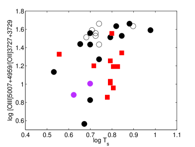
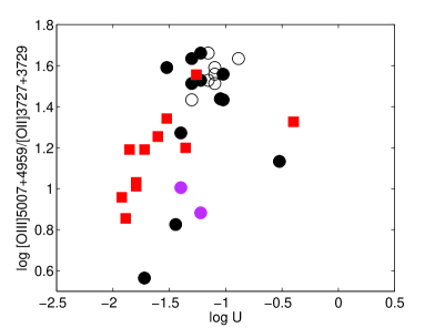
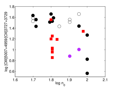
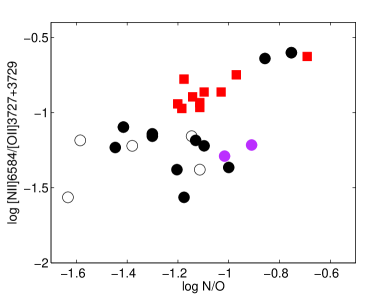
Figure 7: Some significant line ratio trends as function of the different parameters. Black filled circles: galaxies in the 0.020-0.065 z range; black open circles and magenta: galaxies in the 0.020-0.065 z range referring to Table 4 parameters; red filled squares: galaxies in the 0.13-0.43 z range.

5 Concluding remarks

We have collected some significant spectroscopic data observed from star-forming galaxies in the local Universe. We have selected the objects showing a relatively rich spectrum in number of lines from different elements. In particular we have focused on the weak lines such as [OIII]4363, HeII4686, HeI5876, etc. trying to reproduce all the line ratios within each of the observed spectra by the detailed modelling. The results are summarised in the following.

$\bullet$ We confirm that a relatively low metallicity characterizes all the elements, except S. A solar S/H is explained by the contribution to the [SII] lines from the ISM. However, the calculated relative abundances for the other elements (O, N, Ar, etc.) are not as low as evaluated by the observers using the strong line and $\rm T_{e}$ methods.

$\bullet$ A main contribution to the neutral lines (e.g. HeI, [OI]) from the ISM is revealed by comparing calculated to observed line ratios.

$\bullet$ We have found by modelling the observed line ratios that in a not negligible number of galaxies He/H $\leq$0.08 is lower than solar ((He/H)_⊙= 0.1). This result suggests that the wind from the star-forming region not only collisionally affects the dynamics of the emitting cloud throughout the galaxy, but also the gas composition of the emitting clouds.

$\bullet$ For most of the spectra a single model is not enough to fit contemporarily the HeII4686/H${\beta}$  and the [OIII]4363/H${\beta}$  line ratios, whereas the [OIII]5007+/H${\beta}$, [OII]3727+/H${\beta}$, [NII]6584/H${\beta}$  and [NeIII]3868/H${\beta}$  line ratios are all satisfactorily reproduced. The geometrical thickness of the clouds plays a critical role. Pluri-cloud models are adopted in agreement with cloud fragmentation due to turbulence created by the shocks.

$\bullet$ Although by a reduced number of objects, we could assemble some diagrams which can be useful to guess the physical condition and element relative abundance ranges in SF galaxies. In Fig. 7 the trends of the observed line ratios are displayed as function of the calculated parameters. The trends are disturbed because a not negligible number of parameters are interacting with each other. Nevertheless, Fig. 7 diagrams can give some hints to the interpretation of SFG spectra. In the bottom diagrams the trends of the main line ratios are shown for models calculated in the different geometrical thickness ranges in order to point out the role of $D$ in the [OIII]4363/H${\beta}$  and HeII4686/H${\beta}$  modelling.

Data availability

The data underlying my work are available in the manuscript

Appendix A Calculation method

The code suma simulates the physical conditions of an emitting gaseous cloud under the coupled effect of photoionization from a radiation source and shocks assuming a plane-parallel geometry. Two cases are considered relative to the cloud propagation : the photoionizing radiation reaches the gas on the cloud edge corresponding to the shock front (infalling) or on the edge opposite to the shock front (ejection).

To calculate the line flux and the continuum emitted from a gas the physical conditions and the fractional abundances of the ions must be known. In a shock dominated regime the calculations start at the shock front where the gas is compressed and thermalized adiabatically, reaching the maximum temperature (T $\propto$ V${}_{s}^{2}$, where $\rm V_{s}$, is the shock velocity) in the immediate post-shock region. Compression is calculated by the Rankine-Hugoniot equations (Cox 1972) for the conservation of mass, momentum and energy throughout the shock front and downstream. Compression strongly affects the cooling rate and consequently, the distribution of the physical conditions downstream, as well as that of the element fractional abundances. The downstream region is automatically cut in many plane-parallel slabs (up to 300) with different geometrical widths in order to account for the temperature gradient throughout the gas. Thus, the change of the physical conditions downstream from one slab to the next is minimal. In each slab the fractional abundances of all the ions is calculated resolving the ionization equations which account for the ionization mechanisms (photoionization by the primary and diffuse radiation and collisional ionization) and recombination mechanisms (radiative, dielectronic recombinations) as well as charge transfer effects. The ionization equations are coupled to the energy equation (Cox 1972), when collisional processes dominate, and to the thermal balance equation if radiative processes dominate. This latter balances the heating of the gas due to the primary and diffuse radiations reaching the slab and the cooling due to recombinations and collisional excitation of the ions followed by line emission and thermal bremsstrahlung. The coupled equations are solved for each slab, providing the physical conditions necessary to calculate the slab optical depth and the line and continuum emissions. The slab contributions are integrated throughout the nebula. The calculations stop when the electron temperature is as low as 200 K, if the nebula is radiation-bounded or at a given value of the nebula geometrical thickness, if it is matter-bounded. The fractional abundances of the ions are calculated resolving the ionization equations for each element (H, He, C, N, O, Ne, Mg, Si, S, Ar, Cl, Fe) in each ionization level. Then, the calculated line ratios, integrated throughout the cloud thickness, are compared with the observed ones. The calculation process is repeated changing the input parameters until the observed data are reproduced by the model results, at maximum within 10-20 percent.

On this basis we calculate a grid of models. When one or two line ratios underpredict or overpredict the data by a factor of $\geq$ 10, we change drastically the input parameters e.g. the geometrical thickness of the emitting cloud. It is clear that one only set of parameters is not enough to represent the whole galaxy emission. The observations give an average, but an average cannot be fitted by a single spectrum because an average spectrum has not a physical meaning in terms of the line ratios.

The main input parameters of the code are those referring to the shock as well as those characterizing the source ionizing radiation spectrum, and the chemical abundances of He, C, N, O, Ne, Mg, Si, S, Ar, Cl and Fe, relative to H. In our model the line and continuum emitting regions throughout the galaxy cover an ensemble of fragmented clouds. The geometrical thickness of the clouds is an input parameter of the code ($D$) which is calculated consistently with the physical conditions and element abundances of the emitting gas. The effect of dust present in the gas, characterized by the dust-to-gas ratio, $d/g$, and the initial grain radius, a_gr, are also consistently taken into account. The set of selected parameters finally determined for a particular spectrum represents the model.

A.1 Parameters depending on the shock

In the turbulent regime created throughout a starburst (SB) shocks are ubiquitous. The preshock density n₀, the shock velocity $\rm V_{s}$, the magnetic field $\rm B_{0}$ (for all galaxy models $\rm B_{0}$=10^-4Gauss is adopted) represent the shock. They are used in the calculations of the Rankine-Hugoniot equations at the shock front and downstream. They are combined in the compression equation which is resolved throughout each slab of the gas in order to obtain the density profile downstream. Generally, $\rm V_{s}$is constrained by the FWHM of the line profiles, $\rm n_{0}$ by the ratio of the characteristic lines. The relative abundances of the elements are constrained by the line ratios. In the case where shock and photoionization act on opposite sides of a plan-parallel nebula, the geometrical width of the nebula, $D$, is a critical input parameter. The diffuse radiation bridges the two sides, and the smaller $D$ the more entangled are the photoionized and the shocked regions on the opposite sides of the nebula. In this case, a few iterations are necessary to obtain the physical conditions downstream.

A.2 Photoionizing radiation flux

We adopt for the primary radiation a black-body (bb) corresponding to an effective temperature $\rm T_{*}$ and a ionization parameter $U$. A pure bb radiation referring to $\rm T_{*}$ is a poor approximation for a SB, even adopting a dominant spectral type (see Rigby & Rieke 2004). Following Rigby & Rieke, ”the starburst enriches and heats its ISM as well as the intergalactic medium. The ionizing spectrum is set by the SB age, IMF and star formation history.” Adopting a single effective temperature the entire SB field is represented by a single star type. However, the observed line spectra for high redshift galaxies at present cover a narrow optical-near-IR range of frequencies, the lines are few and from few ionization levels, therefore the bb radiation flux calculated by a dominant temperature is acceptable, also in view that the line ratios (that are related to $\rm T_{*}$ ) in a shock dominated regime also depend on the electron temperature, density, ionization parameter, metallicity, on the morphology of the ionized clouds, and in particular, they depend on the hydrodynamical field. Therefore we will determine $\rm T_{*}$ phenomenologically by selecting the effective temperature $\rm T_{*}$ which leads to the best fit of all the observed line ratios for each spectrum and we will use it to calculate the continuum. The primary radiation source does not depend on the physical conditions throughout the galaxy but it affects the surrounding gas. This region is not considered as a unique cloud, but as a sequence of slabs with different thickness calculated automatically following the temperature gradient.

The radiation from a photoionizing source is characterized by its spectrum, which is calculated at 440 energies, from a few eV to KeV, depending on the object studied. Due to radiative transfer, the radiation spectrum changes throughout the downstream slabs, each of them contributing to the optical depth. The calculations assume a steady state downstream. In addition to the radiation from the primary source, the effect of the diffuse secondary radiation created by the gas emission (line and continuum) is also taken into account (see, for instance, Williams 1967), using about 240 energies to calculate the spectrum. The secondary diffuse radiation is emitted from the slabs of gas heated by the radiation flux reaching the gas and by the shock. Primary and secondary radiation are calculated by radiation transfer.

For an AGN, the primary radiation is the power-law radiation flux from the active centre $F$ in number of photons cm^-2 s^-1 eV^-1 at the Lyman limit and spectral indices $\alpha_{UV}$=-1.5 and $\alpha_{X}$=-0.7. $F$ is combined with the ionization parameter $U$ by $U$= ($F$/(n c ($\alpha$ -1)) (($E_{H})^{-\alpha+1}$ - ($E_{C})^{-\alpha+1}$) (Contini & Aldrovandi, 1983), where $E_{H}$ is H ionization potential and $E_{C}$ is the high energy cutoff, $n$ the density, $\alpha$ the spectral index, and c the speed of light.

If the stars are the photoionization source the number of ionizing photons cm^-2 s^-1 produced by the hot source is $N$= $\int_{\nu_{0}}$ $B_{\nu}$/h$\nu$ d$\nu$, where $\nu_{0}$ = 3.29$\times$10¹⁵ s^-1 and B_ν is the Planck function. The flux from the star is combined with $U$ and n by $N$ (r/R)²=$U$nc, where r is the radius of the hot source (the stars), R is the radius of the nebula (in terms of the distance from the stars), n is the density of the nebula and c is the speed of light. Therefore, $\rm T_{*}$ and $U$ compensate each other, but only in a qualitative way, because $\rm T_{*}$ determines the frequency distribution of the primary flux, while $U$ represents the number of photons per number of electrons reaching the nebula. The choice of $\rm T_{*}$ and $U$ is obtained by the fit of the line ratios.

A.3 Electron temperatures through the nebula

The temperature in each slab depends on energy gains (G) and losses (L) of the gas. Close to the shock front downstream, collisional mechanisms prevail and the temperature is calculated from the energy equation in terms of the enthalpy change (Cox 1972). In the slabs where the temperature is $\leq$ 2 10⁴ K, photoionization and heating by both the primary and the secondary radiation dominate and the temperature is calculated by thermal balance (G=L). Gains are calculated by the rate at which energy is given to the electrons by the radiation field (Osterbrock 1974). The energy of suprathermal electrons created by photoionization is rapidly distributed among the thermal electrons through collisions, heating the gas. Several processes contribute to the gas cooling. The cooling rate (Williams 1967) is given by: L = L_ff+L_fb+L_lines+L_dust, where L_ff corresponds to bremsstrahlung, particularly strong at high temperatures and high frequencies. Self-absorption is included in the calculations. L_fb corresponds to free-bound losses due to recombination and is high at T$\leq$ 10⁵ K. L_lines is due to line emission with the bulge between $\leq$ 10⁴ K and 10⁵ K. L_dust represents the energy lost by the gas in the collisional heating of dust grains. It is high the higher d/g and a_gr.

Immediately behind the shock front the gas is thermalized to a temperature of T=1.5 10⁵($\rm V_{s}$/(100 $\rm km\,s^{-1}$))² K. At high temperatures ($\geq$ 10⁶ K) recombination coefficients are very low. The cooling rate is then low. At T between 10⁴ K and 10⁵ K the UV lines and the coronal lines in the IR are strong and lead to rapid cooling and compression of the gas. If the cooling rate is so high to drastically reduce the temperature eluding intermediate ionization-level lines, the calculated spectrum will be wrong. Therefore, the slab thickness must be reduced and all the physical quantities recalculated. The choice of the slab thickness is determined by the gradient of the temperature. This process is iterated until the thickness of the slab is such as to lead to an acceptable gradient of the temperature (T(i-1) - T(i))/T(i-1) $\leq$ 0.1, where T(i) is the temperature of slab i. As the temperature drops, a large region of gas with temperature $\sim$10⁴ K, which is sustained by the secondary radiation, is present in the radiation-bounded case, i.e. when the gas recombines completely before reaching the edge of the nebula opposite to the shock front. Due to a lower temperature gradient, calculations in this zone may be performed in slabs with a larger geometrical thickness.

A.4 Element abundances

We start model calculations by adopting solar abundances. We use solar abundances which are intermediate between those presented by Anderson & Grevesse (1989) and Asplund et al (2009), similar to those of Allen (1976) for all the elements, in particular for oxygen, trying to fit the observations. If the [OIII]5007+/H${\beta}$, [OIII]4363/H${\beta}$  and [OII]/H${\beta}$  line ratios all satisfactorily reproduce the data, we adopt for O/H the solar value. If the the oxygen lines ratios to H${\beta}$  are all higher (or lower) than observed by a similar factor, we try to reproduce all the oxygen line ratios to H${\beta}$  by reducing (or increasing) O/H. If the various oxygen line ratios to H${\beta}$  differ from the data by different factors we restart the modelling process by changing all the input parameter set. When the oxygen to H${\beta}$  line ratios reproduce successfully the data, we change the other element relative abundances, in particular N/H and S/H, if necessary. The oxygen abundance, in particular, strongly affects the cooling rate downstream in the recombination zone throughout the emitting clouds. Therefore, the calculations process must be reinitiated until the best fit of all the line ratios to H${\beta}$  from all the elements is obtained.

In particular, the absolute line fluxes referring to the ionization level i of element K are calculated by the term $n_{K}$(i) which represents the density of the ion i. We consider that $n_{K}$(i)=X(i)[K/H]$n_{H}$, where X(i) is the fractional abundance of the ion i calculated by the ionization equations, [K/H] is the relative abundance of the element K to H and $n_{H}$ is the density of H (by number $\rm cm^{-3}$). In models including shock, $n_{H}$ is calculated by the compression equation in each slab downstream. So the abundances of the elements are given relative to H as input parameters.

A.5 Dust grain heating

Dust grains are coupled to the gas across the shock front by the magnetic field (Viegas & Contini 1994). They are heated by the radiation source and collisionally by the gas to a maximum temperature which is a function of the shock velocity, of the chemical composition and of the radius of the grains, up to the evaporation temperature ($T_{\rm dust}$ $\geq$ 1500 K). The grain radius distribution downstream is determined by sputtering, which depends on the shock velocity and on the density. Throughout shock fronts and downstream, the grains might be destroyed by sputtering. The grains are heated by the primary and secondary radiation, and by gas collisional processes. Details of the calculations of the dust temperature are given by Viegas & Contini (1994). When the dust-to-gas ratio $d/g$ is high, the mutual heating of dust and gas may accelerate the cooling rate of the gas by L_dust, changing the line and continuum spectra emitted from the gas. The intensity of dust reprocessed radiation in the IR depends on $d/g$ and on the radius a_gr. In this work we use $d/g$=10^-14 by number for all the models which corresponds to 4.1 10^-4 by mass for silicates.

References

- Aldrovandi (1985) Aldrovandi, S.M.V. & Contini, M. 1985 A&A, 149, 109
- Allen (1976) Allen, C.W. 1976 in Astrophysical Quantities, London: Athlone(3rd edition)
- Allen (2008) Allen, M.G., Groves, B.A., Dopita, M.A., Sutherland, R.S., Kewley, L.J. 2008, ApJS, 178, 20
- Anderson (1989) Anderson, E. & Grevesse, N. 1989, Geochimica and Cosmochimica Acta, 53, 197
- Asplund (2009) Asplund, M., Grevesse, N., Sauval, A. J., Scott, P. 2009, ARA&A, 47,481
- Baldwin (1981) Baldwin, J.A., Phillips, M.M., Terlevich, R. 1981, PASP, 93,5
- Barstow (1994) Barstow, M.A. 1994, MNRAS, 271, 175
- Berg (2012) Berg, D.A. et al 2012, ApJ, 754, 98
- Berg (2016) Berg, D.A., Skillman, E.D., Henry, R.B.C., Erb, D.K., Carigi, L. 2016, ApJ, 826, 21
- Congiu (2017) Congiu, E. et al, 2017 MNRAS, 471, 562
- Contini (2017) Contini M., 2017, MNRAS, 469, 3125
- Contini (2016) Contini, M. 2016, MNRAS, 461, 2374
- Contini (2014) Contini, M. 2014, A&A, 564, 19
- Contini (2009) Contini, M. 2009, MNRAS, 399, 1175
- Contini (1997) Contini, M. 1997, A&A, 323, 71
- Cox (1972) Cox, D.P. 1972, ApJ. 178. 1159
- Ekta (2010) Ekta,B. & Chengalur, J.N. 2010, MNRAS, 406, 1238
- Faria (2021) Fonseca-Faria, M.C., Rodriguez-Ardila, A., Contini, M., Reynaldi, V. 2021, MNRAS, 506, 783
- Ferland (2017) Ferland, G.J. et al 2017, Rev. Mex. Astr., 53, 335
- Guseva (2020) Guseva, N.G. , Izotov, Y.i. , Schaerer, D. , Vilchez, J.M.V., Amorin, R., Perez-Montero, E., Iglesias-Paramo, J., Verhamme, A., Kehrig, C., Ramambason, L. 2020, MNRAS, 497, 4293 (G20)
- Hayden (2021) Hayden-Pawson, E. et al 2021 arXiv:2110.00033
- Henry (2000) Henry, R.B.C., Edmunds, M.G. & Köppen, J. 2000, ApJ, 541, 660
- Izotov (1997) Izotov, Y.I., Lipovetsky, V.A., Chaffe, F.H., Foltz, C.B., Guseva, N.G., Kniazev, A.Y. 1997, arXiv: astro-ph/9607119
- Izotov (1999) Izotov, Y.I., Thuan, T.X., 1999, 511, 639
- Izotov (2006) Izotov, Y.I., Schaerer, D., Blecha, A., Royer, F., Guseva, N.G., North, P. 2006, arXiv:astro-ph/0608203
- Izotov (2012) Izotov, Y.I., Thuan, T.X., Guseva, N.G., 2012 A&A, 546, 129
- Izotov (2020) Izotov, Y.I., Schaerer, D., Worseck, G., Verhamme, A., Guseva, N. G., Thuan,T.X., Orlitova,I., Fricke, K. J. 2020, MNRAS, 491, 4681 (I20)
- Izotov (2019b) Izotov, Y.I., Thuan, T.X., Guseva, N.G. 2019, MNRAS, 483, 5491, (I19b)
- Izotov (2019a) Izotov, Y. I.; Guseva, N. G.; Fricke, K. J.; Henkel, C. 2019, A&A, 623, 40, (I19a)
- Izotov (2018b) Izotov, Y. I. ; Worseck, G.; Schaerer, D.; Guseva, N. G.; Thuan, T. X.; Fricke, Verhamme, A.; Orlitova, I. 2018, MNRAS, 478, 4851 (I18b)
- Izotov (2018a) Izotov, Y.I., Thuan, T.X., Guseva, N.G., Liss, S.E. 2018, MNRAS, 473, 1956 (I18a)
- Izotov (2021) Izotov, Y.I., Thuan, T.X., Guseva, N.G. 2021, MNRAS, 5004, 3996
- kauffmann (2003) Kauffmann, G. et al. 2003, MNRAS, 341, 33
- kewley (2001) Kewley, L.J., Dopita, M.A., Sutherland, R.S., Heisler, C.A., Trevena, J. 2001, ApJ, 556, 121
- Lauffer (2018) Lauffer, G.R., Romero, A.D., Kepler, S.O. 2018, MNRAS, 480, 1547
- lyubymkov (2018) Lyubymkov, L.S. 2018, ArXiv:1809.06129
- Marino (2013) Marino, R.A. et al. 2013, A&A, 559, 114
- Mont (2021) Monteiro, A.F., Dors, O.L. 2021, MNRAS.temp.2508M
- Morton (1968) Morton, D.C. 1968, ApJ, 151, 285
- Osterbrock (1974) Osterbrock, D.E. 1974 in Astrophysics of Gaseous Nebulae, San Francisco, W.H.Freeman and Co., 1974
- Perez (2005) Pérez-Montero, E., Diaz, A.I. 2005, MNRAS, 361, 1063
- Perez (2011) Pérez-Montero, E. et al. 2011, A&A, 532, 141
- Perez (2013) Pérez-Montero, E. et al. 2013, A&A, 549, A25
- Pustilnik (2004) Pustilnik, S.; Kniazev, A.; Pramskij, A.; Izotov, Y.; Foltz, C.; Brosch, N.; Martin, J. -M.; Ugryumov, A. W. 2004, A&A, 419, 469 (P04)
- Rigby (2004) Rigby, J.R. & Rieke, G.H. 2004, ApJ, 606, 237
- Rupke (2005) Rupke, D.S., Veilleux, S., Sanders, D.A. 2005, ApJ, 160, 115
- Schaerer (2019) Shaerer, D., Fragos, T., Izotov, Y.I. 2019, A&A, 622, L10
- Yu (2021) Yu,B.P.B., Owen, E.R., Pan, K.-C., Wu, K., Ferreras, I. 2021, arXiv:2109.09764
- Viegas (94) Viegas, S.M., Contini, M. 1994, ApJ, 428, 113
- Williams (67) Williams, R.E. 1967, ApJ, 147, 556