Numerical evaluation of ODE solutions by Monte Carlo enumeration of Butcher series
Abstract
We present an algorithm for the numerical solution of ordinary differential equations by random enumeration of the Butcher trees used in the implementation of the Runge-Kutta method. Our Monte Carlo scheme allows for the direct numerical evaluation of an ODE solution at any given time within a certain interval, without iteration through multiple time steps. In particular, this approach does not involve a discretization step size, and it does not require the truncation of Taylor series.
Keywords: Ordinary differential equations, Runge-Kutta method, Butcher series, random trees, Monte Carlo method.
Mathematics Subject Classification (2020): 65L06, 34A25, 34-04, 05C05, 65C05.
1 Introduction
Butcher series [But63], [But16] are a powerful tool used to represent the Taylor expansions appearing in the Runge-Kutta methods for the numerical solution of ordinary differential equations (ODEs), see Chapters 4-6 of [DB02], and [MMMKV17] for a recent review starting from the early work of [Cay57]. Those series are making use rooted tree enumeration, which have many applications ranging from geometric numerical integration to stochastic differential equations, see for instance [HLW06] and references therein, and [Gub10], [BHZ19], [Fos21] for the use of decorated trees for stochastic partial differential equations and their connections with the Butcher-Connes-Kreimer Hopf algebra [CK99].
It is known that the solution of the autonomous -dimensional ODE system
| (1.1) |
where is a smooth d-valued function of in a domain of d, can be expressed as
| (1.2) |
where we use the notation
| (1.3) | ||||
| (1.4) | ||||
| (1.5) |
etc. In addition, the expansion (1.2) can be coded and enumerated using the following sequence of Butcher trees, which can also be represented without referring to the derivatives of , see for example Table 1.1 page 53 of [HLW06].
| Order | Coefficient | Butcher tree | Order | Coefficient | Butcher tree | Order | Coefficient | Butcher tree |
| 0 | 1 |
|
2 |
|
||||
| 3 |
|
3 |
|
The numerical evaluation of Butcher series involves tree enumeration up to a certain order that determines the level of precision of the algorithm.
In this paper, we propose an alternative method to the numerical evaluation of ODE solutions, based on a random enumeration of Butcher trees by Monte Carlo simulation. Probabilistic methods based on the Feynman-Kac formula provide alternatives to finite difference schemes, and have been successfully applied to the solution of partial differential equations. In particular, stochastic branching mechanisms have been used to represent the solutions of partial differential equations in [Sko64], [INW69], [NS69], [McK75], [LM96], [CLM08]. This branching argument has been recently extended in [HLOT+19] to the treatment of polynomial non-linearities in gradient terms, see also [PP22] for nonlocal and fractional PDEs.
In Theorem 4.2, under suitable integrability conditions we express ODE solutions as the expected value of a functional of random Butcher trees which encode nonlinearities. Then in Proposition 4.3 we provide sufficient conditions ensuring that the representation formula of Theorem 4.2 holds at any time within certain interval. Numerical values of ODE solutions can be computed beyond that initial interval by iterating the method and by piecing together the solutions obtained on adjacent intervals. As noted before Proposition 4.3, the integrability conditions are stronger in higher dimensions.
This approach complements the use of the Feynman-Kac formula for the numerical estimation of the solutions of partial differential equations, see also [SH21] for a different approach to the Feynman-Kac representation of ODE solutions. Other links between Butcher trees and probability theory have been pointed out in [Maz04], see also [Ski92] for the numerical solution of ODEs as an inference problem by Bayesian techniques.
In comparison with integrators in the Runge-Kutta method, our method requires the evaluation of and its partial derivatives up to any order, whereas the Runge-Kutta method uses only . The complexity of our algorithm grows linearly with dimension, as trees are used to solve a -dimensional ODE system, whereas the complexity of finite difference methods is generally polynomial in the dimension , depending on the order chosen in the truncation of (1.2). Complexity in time can be estimated via the mean length of binary trees, which grows exponentially in time independently of dimension in the case of exponentially distributed branch lifetimes, as noted in Section 4. On the other hand, our method can be used to exactly approximate the solution at any given time on a (possibly infinite) time interval. Our approach also benefits from the advantages of Monte Carlo estimators whose computation can be paralleled straightforwardly.
In Section 2 we introduce the construction of coding trees that will be used for the numerical solution of ODEs. Section 4 presents the probabilistic representation formula of ODE solutions obtained by the random generation of coding trees. In Section 5 we consider examples and in Section 6 we describe the correspondance between Butcher trees and coding trees, namely we show how any Butcher tree can be recovered by performing a depth first search on the corresponding coding tree, showing how Butcher series can be rewritten as series of expected values. Section 7 considers numerical applications, and the appendix contains the corresponding computer codes in Maple, Mathematica and Python.
2 Codes and mechanism
This section introduces the random coding trees used for the probabilistic representation of ODE solutions. We consider a multidimensional autonomous system of the form
| (2.1) |
, where is a smooth Lipschitz function defined on a domain of , . In order to solve (2.1) iteratively, we can start by expanding as
| (2.2) |
by differentiating , where we use the notation , . In the sequel, given a function from d into , we let denote the mapping
| (2.3) |
where represents the set of functions from + to d. In order to formalize and extend the iteration initiated in (2.2), we introduce the following definitions. In the sequel we let denotes the - canonical projection from to with , .
Definition 2.1
We let denote the set of functions from to called codes, defined as
By (2.3), the elements of are operators mapping a function to another function . We also consider a mapping , called the mechanism, defined on by matching a code to a set of code tuples.
Definition 2.2
The mechanism is defined by and
| (2.4) |
for a smooth function from d into .
In the next key lemma we show that satisfies a system of equations indexed by .
Lemma 2.3
For any code we have
| (2.5) |
We note that for any it is always possible to compute by applying the code to the solution of the ODE and then evaluating it at time as . In particular, the full knowledge of the function is not necessary to compute .
Example - One-dimensional autonomous ODE
Consider the solution of the one-dimensional ODE
where is expanded as
Here, denotes the mapping
for a smooth function from to , the set of codes is given by
where , , denotes the operator acting as
and the mechanism is given by and .
Example - Non-autonomous ODE
Consider the non-autonomous ODE
| (2.6) |
where is a smooth Lipschitz function defined on a domain of . This ODE can be rewritten as the system
| (2.7) |
by taking and , . Here, the set of codes satisfies
where and denote constant functions. The mechanism is given by , , and for a smooth function from 2 into .
More generally, any non autonomous system can be transformed into an autonomous system by addition of a dimension. In particular, any higher order ordinary differential equation of the form
can be written as a system of the form (2.1) by taking , , and , with and , .
3 Coding trees
For each code we denote by a uniformly distributed random variable on . For example, when , since , we have
In the sequel we will use the notation
In addition, we consider a probability density function and
-
•
an i.i.d. family of random variables with distribution on +,
-
•
for each , an i.i.d. family of discrete random variables, with
where the sequences and are assumed to be mutually independent. For every we also consider an injection .
Let . For each we construct a random tree starting from an initial particle labelled bearing the code at time , which lives up to a random time distributed according to . If , the branching process stops. Otherwise, if , a new particle with label is created, and bears the code since , and independently follows the same pattern as the first one. This new branch lives during the time . If then the tree stops branching, otherwise, if , the particle branches in two branches chosen uniformly in .
More generally, a particle with code at the generation is assigned a label of the form , while its parent label is . The birth time of particle is denoted by , and its lifetime is the element of index in the i.i.d. sequence . If , we draw a sample uniformly in with , and the particle branches into offsprings at generation , which are labeled by , . The particle with label ending with an integer will carry the code . Finally, the code of particle will be denoted by . The death time of the particle is , and its birth time is .
Definition 3.1
We denote by the random tree constructed from the above argument started from any code .
The family of trees will be used for the stochastic representation of the solution of the ODE system (2.1), while the trees will be used for the stochastic representation of . The next table summarizes the notation introduced so far.
| Object | Notation |
|---|---|
| Initial time | |
| Tree ending at time with initial code | |
| Particle (or label) of generation | |
| First branching time | |
| Birth time of a particle | |
| Death time of a particle | |
| Lifespan of a particle | |
| Code of a particle |
The following graph represents a sample of the random tree , .
4 Probabilistic representation of ODE solutions
In this section we define the random multiplicative functional which will be used to represent ODE solutions. We let denote the tail distribution function of , i.e.
We denote by the set of particles that do not live until time , and by the set of particles that die after time .
Definition 4.1
Given a random coding tree started with the code and ending at time , we define the universal multiplicative functional by
The next result gives the probabilistic representation of ODE solutions as an expected value over random coding trees.
Theorem 4.2
Let for which there exists such that
Then, for any we have the probabilistic representation
| (4.1) |
where is the solution of the system of ODEs (2.1). In particular, taking , we have
Proof. For we let
By conditioning on the first branching time , for all the first particle bearing the code branches at time into a new particle bearing the code as , hence we have
Similarly, starting from any code different from , the particle branches at time in possible different ways into two particles with codes , , hence we have
| (4.2) |
which yields the system of equations
| (4.3) |
By the Cauchy-Lipschitz theorem on the Banach space of sequences , this system admits a unique maximal solution. We conclude by noting that from Lemma 2.3, the family of functions is the solution of the system (4.3), hence , and
In numerical applications the expected value in Theorem 4.2 is estimated as the average
where are independent samples of . In this case, the error on the estimate of from the Monte Carlo method can be estimated as the standard deviation
Complexity of the algorithm
We note that the complexity of the algorithm grows linearly with the dimension , as trees are used to generate the multidimensional solution , whereas the complexity of finite difference methods is generally polynomial in the dimension , depending on the order chosen in the truncation of (1.2). On the other hand, all trees are at most binary regardless of the dimension , as shown by the construction (2.4) of the mechanism .
Regarding complexity in time, let denote the mean size of the random tree generated until time , with, by construction, for all , and for all . The same argument as in the proof of Theorem 4.2 shows that satisfies the sytem of integral equations
When has the exponential density with parameter , this leads to the system
with solution
and where is a standard Poisson process with intensity . We note that this estimate remains the same independently of dimension .
Integrability condition
The following proposition provides sufficient conditions ensuring that the representation formula (4.1) of Theorem 4.2 holds at any time within certain interval. In order to represent an ODE solution beyond that time interval we may reuse the numerical value obtained close to its boundary as new initial condition in order to represent the solution on an extended time interval. We note that the constant in the next proposition depends on and and its derivatives, and is independent of the system dimension . However, the integrability condition (4.4) is stronger in higher dimensions.
Proposition 4.3
Assume that there exists such that for any , that the density function is nonincreasing, and that
| (4.4) |
Then, there exists such that
| (4.5) |
We note that trying to relax the integrability condition (4.4) by choosing a higher will result into a smaller value of , therefore increasing the time complexity of the algorithm. On the other hand, assuming that
yields the system of equations
Since the corresponding trees , have same random shape distribution, we have for all codes such that , , . This gives the system
which can be solved as
hence the finiteness of holds at most until time
| (4.6) |
Remark 4.4
Although the non-autonomous ODE (2.6) can be treated using an autonomous -dimensional system of the form (2.7), the probabilistic representation (4.1) of its solution can also be obtained using a single random tree. For this, we expand as
In this case, the set of codes is defined as
and the mechanism is given by
A sample of this random tree is presented below.
In this case, the system of equations satisfied by can be written as
which can be solved as
Therefore, the finiteness of holds until time
| (4.7) |
Under the conditions and , since , we have
hence
In this setting the integrability condition (4.7) is stronger than (4.6) when is sufficiently large, and weaker otherwise. On the other hand, in comparison with the autonomous system (2.7), time complexity of the algorithm is divided by at least two due the use of a single coding tree with less branches.
5 Examples
Exponential series
We first consider the equation
rewritten in integral form as
whose solution admits the power series expansion
Here we have , and the mechanism satisfies . The particle of generation bears the label , and its parent is the particle . When the random times are independent and exponentially distributed, i.e. with , the total number of branches in the random tree is given by where is a standard Poisson process with unit intensity.
In this case, the multiplicative functional
simplifies to the deterministic expression
in which we take and .
One-dimensional autonomous ODE
Consider the autonomous ODE
| (5.1) |
where is bounded together with its derivatives of order , with
for some . For any we have the integral equation
with the set of codes , and the mechanism is defined by
Below is a representation of a sample of the random tree .
With , , the system (4.2) reads
6 Mapping of coding trees to Butcher trees
In this section we describe the connection between coding trees, Butcher series and Butcher trees, by showing how any Butcher tree can be recovered by performing a depth first search on the corresponding coding trees. The solution of the -dimensional ODE system (1.1) is written as the Butcher series
| (6.1) |
where the above summation over Butcher trees is formal and may not converge. Here, the order denotes the number of vertices of the tree , is a term also depending on the derivatives of at as in (1.3)-(1.5), and is a coefficient which is defined recursively, see Relation (4) in [But10].
Proposition 6.1
Every Butcher tree can be mapped to a unique tree , so that the Butcher series (6.1) can be rewritten as
where the notation means that the coding tree has the tree structure .
Proof. The one-to-one mapping is constructed by performing a depth first search on coding trees, as illustrated in the following examples which show how any Butcher tree of order can be mapped to a unique tree generating coding trees . Namely, every Butcher tree can be recovered by performing a depth first search on the corresponding coding tree by matching leaves on Butcher trees to branches of the same color in coding trees.
If a node in the initial coding tree branches into two new coding trees (above) and (below), the Butcher tree for the initial coding tree is obtained by sticking the Butcher tree obtained from to the root of the Butcher tree obtained from . If a tree is a leaf with code of the form with , then the corresponding Butcher tree has a single node containing .
| Order | Butcher tree | Coding trees | |
|---|---|---|---|
| 1 |
|
|
| Order | Butcher tree | Coding trees | |
|---|---|---|---|
| 2 |
|
|
| Order | Butcher tree | Coding trees | |
|---|---|---|---|
| 3 |
|
| 3 |
|
|
| Order | Butcher tree | Coding trees | |
|---|---|---|---|
| 4 |
|
| 4 |
|
|
| 4 |
|
|
| 4 |
|
|
When is a Butcher tree of order , based on the construction of on page 155 of [But10], the - component of the term in the expansion of is a sum of and its partial derivatives at as in (1.3)-(1.5). This sum can be interpreted as a sum of over , weighted by the probability coefficients
and integrated over the branching times , which yields the identity
7 Numerical application
In this section we consider various ODE examples with different choices of probability density functions satisfying (4.4), or under (4.6). The errors observed in Figures 3, 4, 5, only occur at a time threshold after which the estimator is no longer integrable and the estimates are unreliable. The following graphs are plotted with one million Monte Carlo samples.
-
i)
Taking , we start with the quadratic ODE
(7.1) with solution
In the framework of (5.1) we have
hence we have for all , and in agreement with (4.6) the representation formula (4.1) of Theorem 4.2 holds for , see Figure 1. In this example and in the next two examples we take to be the exponential probability density function , .
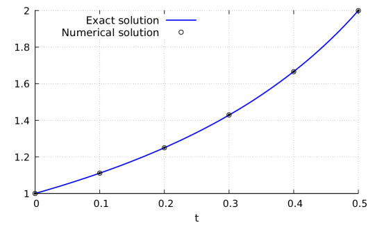
Figure 1: Numerical solution of (7.1) with . -
ii)
Next, we take and consider the equation
(7.2) with solution
in the framework of (5.1). When we have , and in agreement with (4.6) the representation formula (4.1) of Theorem 4.2 holds for , see Figure 2.
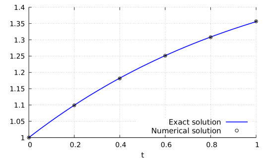
Figure 2: Numerical solution of (7.2). -
iii)
Taking we find Equation (201a) in [But16], i.e.
(7.3) with solution
In this case, the time interval of validity may not be determined explicitly because and the finiteness of this supremum is only a sufficient condition for (4.5) to hold in Proposition 4.3. Figure 3 shows the convergence of the Monte Carlo algorithm until .
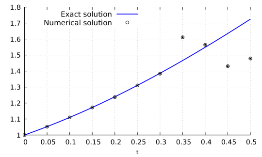
Figure 3: Numerical solution of (7.3). -
iv)
Taking yields Equation (316e) in [But16], i.e.
(7.4) whose solution is given in parametric form as . As in Example iii) above, the time interval of validity may not be determined explicitly, see Figure 4. In this example and in the next one, we take to be the gamma probability density function , .
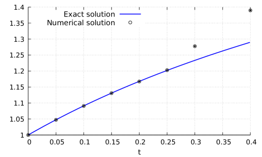
Figure 4: Numerical solution of (7.4). -
v)
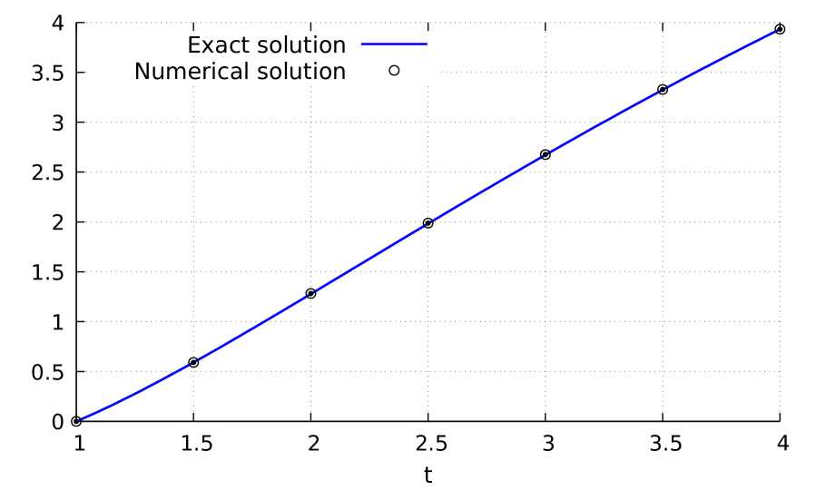
Taking we find Equation (223a) in [But16], i.e.
(7.5) with solution
In this case we have , and in agreement with (4.6) the representation formula (4.1) of Theorem 4.2 is valid on the time interval , see Figure 5.
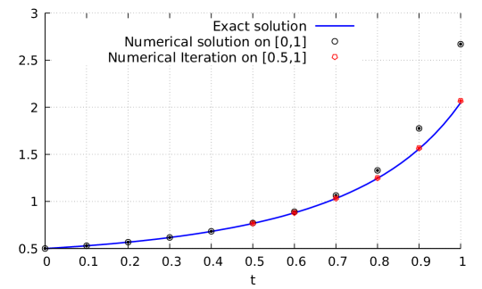
Figure 5: Numerical solution of (7.5). In addition, after running the algorithm on the time interval we may reuse the numerical evaluation at time as a new initial condition and iterate the algorithm on the time interval with more precise estimates, as shown in red in Figure 5. We refer to this procedure as “patching”.
-
vi)
Consider the ODE system (316f) page 177 in [But16], i.e.
(7.6) with solution
The graphs of Figure 6 are obtained using the Python code provided in appendix, where we patch the algorithm times over the time interval and take to be the exponential probability density function , .
(a) Graph of . 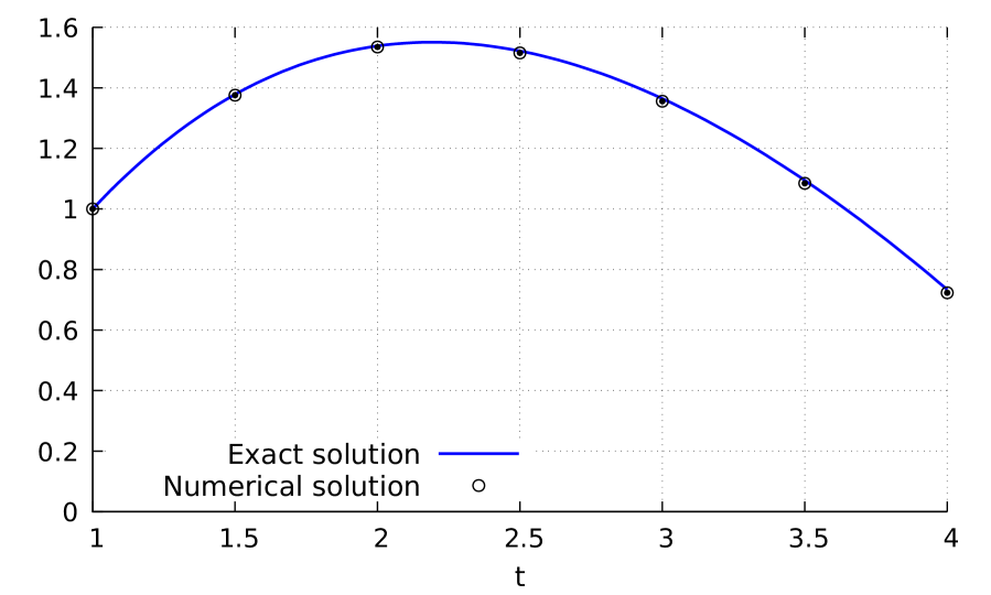
(b) Graph of . Figure 6: Numerical solution of (7.6).
Appendix A Computer codes
The following Maple and Mathematica codes implement the algorithm of Theorem 4.2 for one-dimensional non-autonomous ODEs using the exponential distribution , .
The following Python code implements the algorithm of Theorem 4.2 for systems of ODEs.
Acknowledgement
We thank Jiang Yu Nguwi for producing the Python code dealing with systems of ODEs.
References
- [BHZ19] Y. Bruned, M. Hairer, and L. Zambotti. Algebraic renormalisation of regularity structures. Invent. Math., 215:1039–1156, 2019.
- [But63] J.C. Butcher. Coefficients for the study of Runge-Kutta integration processes. J. Austral. Math. Soc., 3:185–201, 1963.
- [But10] J.C. Butcher. Trees and numerical methods for ordinary differential equations. Numerical Algorithms, 53:153–170, 2010.
- [But16] J.C. Butcher. Numerical methods for ordinary differential equations. John Wiley & Sons, Ltd., Chichester, third edition, 2016.
- [Cay57] A. Cayley. On the theory of the analytical forms called trees. Philosophical Magazine, 13(85):172–176, 1857.
- [CK99] A. Connes and D. Kreimer. Lessons from quantum field theory: Hopf algebras and spacetime geometries. Letters in Mathematical Physics, 48:85–96, 1999.
- [CLM08] S. Chakraborty and J.A. López-Mimbela. Nonexplosion of a class of semilinear equations via branching particle representations. Advances in Appl. Probability, 40:250–272, 2008.
- [DB02] P. Deuflhard and F. Bornemann. Scientific Computing with Ordinary Differential Equations, volume 42 of Texts in Applied Mathematics. Springer-Verlag, New York, 2002.
- [Fos21] L. Fossy. Algebraic structures on typed decorated rooted trees. SIGMA, 17:1–28, 2021.
- [Gub10] M. Gubinelli. Ramification of rough paths. J. Differential Equations, 248(4):693–721, 2010.
- [HLOT+19] P. Henry-Labordère, N. Oudjane, X. Tan, N. Touzi, and X. Warin. Branching diffusion representation of semilinear PDEs and Monte Carlo approximation. Ann. Inst. H. Poincaré Probab. Statist., 55(1):184–210, 2019.
- [HLW06] E. Hairer, C. Lubich, and G. Wanner. Geometric numerical integration, volume 31 of Springer Series in Computational Mathematics. Springer-Verlag, Berlin, second edition, 2006.
- [INW69] N. Ikeda, M. Nagasawa, and S. Watanabe. Branching Markov processes I, II, III. J. Math. Kyoto Univ., 8-9:233–278, 365–410, 95–160, 1968-1969.
- [LM96] J.A. López-Mimbela. A probabilistic approach to existence of global solutions of a system of nonlinear differential equations. In Fourth Symposium on Probability Theory and Stochastic Processes (Spanish) (Guanajuato, 1996), volume 12 of Aportaciones Mat. Notas Investigación, pages 147–155. Soc. Mat. Mexicana, México, 1996.
- [Maz04] C. Mazza. Simply generated trees, -series and Wigner processes. Random Structures Algorithms, 25(3):293–310, 2004.
- [McK75] H.P. McKean. Application of Brownian motion to the equation of Kolmogorov-Petrovskii-Piskunov. Comm. Pure Appl. Math., 28(3):323–331, 1975.
- [MMMKV17] R.I. McLachlan, K. Modin, H. Munthe-Kaas, and O. Verdier. Butcher series: a story of rooted trees and numerical methods for evolution equations. Asia Pac. Math. Newsl., 7(1):1–11, 2017.
- [NS69] M. Nagasawa and T. Sirao. Probabilistic treatment of the blowing up of solutions for a nonlinear integral equation. Trans. Amer. Math. Soc., 139:301–310, 1969.
- [PP22] G. Penent and N. Privault. Existence and probabilistic representation of the solutions of semilinear parabolic PDEs with fractional Laplacians. Stochastics and Partial Differential Equations: Analysis and Computations, 10:446–474, 2022.
- [SH21] Z. Selk and H. Harsha. A Feynman-Kac type theorem for ODEs: Solutions of second order ODEs as modes of diffusions. Preprint arXiv:2106.08525, 16 pages, 2021.
- [Ski92] J. Skilling. Bayesian solution of ordinary differential equations. In C. R. Smith, G. J. Erickson, and P. O. Neudorfer, editors, Proceedings of the Eleventh International Workshop on Maximum Entropy and Bayesian Methods of Statistical Analysis, volume 50 of Fundamental Theories of Physics, pages 23–38. Kluwer Academic Publishers Group, Dordrecht, 1992.
- [Sko64] A.V. Skorokhod. Branching diffusion processes. Teor. Verojatnost. i. Primenen., 9:492–497, 1964.