[$\ddagger$]xxThese authors contributed equally e1 e2 e3

The functional renormalization group (FRG), an established computational method for quantum many-body phenomena, has been subject to a diversification in topical applications, analytic approximations and numerical implementations. Despite significant efforts to accomplish a coherent standard through benchmarks and the reproduction of previous results, no systematic and comprehensive comparison of different momentum space FRG implementations has been provided until now. While this has not prevented the publication of relevant scientific results we argue that established mutual agreement across realizations will strengthen confidence in the method. To this end we report explicit implementational details and numerical data reproduced thrice independently up to machine accuracy. To substantiate the reproducibility of our calculations we scrutinize pillar FRG results reported in the literature, and discuss our calculations of these reference systems. We mean to entice other groups to reproduce and establish this set of benchmark FRG results thus propagating the joint effort of the FRG community to engage in a shared knowledge repository as a reference standard for FRG implementations

Reference results for the momentum space functional renormalization group

1 Introduction

The functional renormalization group (FRG) is one of the most promising methods for the analysis of low-temperature instabilities of two dimensional materials  dlpena_lichtenstein_honerkamp2017 ; pena-scherer-2017 ; o_competing_2021 ; korea_graphene_2019 ; klebl-kennes-honerkamp-2020 ; hauck_honerkamp_kennes-2021 ; classen-honerkamp-scherer-2019 ; kiesel-thomale-ea-2012 ; wang-frg-graphene-2012 ; dlpena_scherer_honerkamp_2014 ; Classen-2014-phonon ; kennes2018strong ; honerkamp-honeycomb-2008 ; raghu-topological-2008 ; wang-FeAs-2009 ; wolf2021triplet as it offers an unbiased view, not presupposing the existence of certain phase transitions metzner-salmhofer-honerkamp-2012 . Because the numerics involved in prediction using the FRG are expensive, the full breadth of possible dependencies could only be captured by a few implementations of the two-dimensional single-band Hubbard model on the square lattice tagliavini-ea-2019-multiloop ; hille-ea-2020-quantitative , while a generalization to non-$SU(2)$ symmetric or multi-orbital models is still absent. This inherent fragmentation has rendered it difficult to directly compare distinct implementations. Traditionally only qualitative results have been employed lichtenstein_high-performance_2017 . Unfortunately various qualitative features produced by the FRG, such as the critical scale and leading instabilities, have (over the course of converging our three distinct implementations) proven to be robust against a certain degree of programming error e.g. the exact ordering of indices in subleading diagrams. When trying to predict many-body instabilities of novel systems, certainty over reference calculations is crucial to assure validity. Beyond the qualitative level, the aspiration of the method is to become a quantitative quantum many-body tool, further emphasizing numerical correctness. The definition of correctness here refers to a certain formal approximation level, i.e. a specific truncation of the hierarchy of FRG equations, as detailed in Ref. metzner-salmhofer-honerkamp-2012 . When gauging the physical potential of a certain approximation or comparing various approximations, validity of numerical implementations is mandatory. It is therefore desirable to introduce a shared knowledge of the “proper” results of the tensor contractions intrinsic to most FRG calculation. A reproduction of the exact numerics yields certainty over prefactors, signs as well as contraction indices, not ensured when validating using e.g. the phase transitions predicted in the square lattice Hubbard model. We try to lay the groundwork for achieving consistency across different codes by providing momentum-space data of the frequency independent interaction vertex reproduced by three different, independently developed FRG codes. We choose this focus as a first step towards a shared knowledge repository, motivated by the application to strongly correlated states in two-dimensional materials.

The paper is structured as follows: We first give a short briefing on the theory and some technicalities of the momentum-space FRG and its truncated unity formfactor expansion. Then we introduce the three distinct implementations and elaborate their areas of application. We proceed to provide results in the three tests systems we have chosen, in order to establish agreement with published references. The penultimate section presents the exact procedure of our comparison, enabling the reader to compare their own implementation using the provided parameter and data sets. Intricacies and specifics regarding various challenges faced during development are presented in the Appendix.

2 Method

2.1 Functional Renormalization Group

The derivation of FRG is given in utmost brevity here, we refer the interested reader to Refs. metzner-salmhofer-honerkamp-2012 ; Dupuis_review_2021 for an in-depth discussion. We commence with the partition function of the interacting system:

$$\mathcal{Z}=\int\mathcal{D}\psi\mathcal{D}\bar{\psi}\,e^{-S[\psi,\bar{\psi}]}\,,$$ (1)

where $\psi,\bar{\psi}$ are fermionic Grassmann fields and $S$ is the action of the system given by single-particle and interacting components:

$$S[\psi,\bar{\psi}]=-(\bar{\psi},Q_{0}\psi)+S_{I}[\psi,\bar{\psi}]\,.$$ (2)

Here $Q_{0}=ik_{0}-H_{0}+\mu=G_{0}^{-1}$ denotes the inverse of the bare one-particle Green’s function with $H_{0}$ as the non-interacting part of the Hamiltonian, $k_{0}$ a Matsubara frequency and $\mu$ the chemical potential.

By adding external sources $\eta,\bar{\eta}$ and Legendre transforming we obtain the generating functional, the logarithm of which is the generating functional for connected Green’s functions, $\mathcal{W}[\eta,\bar{\eta}]$. The effective action $\Gamma[\psi,\bar{\psi}]$ is then obtained by another Legendre transform of $\mathcal{W}[\eta,\bar{\eta}]$:

$$\begin{split}&\mathcal{W}[\eta,\bar{\eta}]=-\mathrm{ln}\int\mathcal{D}\psi\mathcal{D}\bar{\psi}\,e^{-S[\psi,\bar{\psi}]+(\bar{\eta},\psi)+(\eta,\bar{\psi})}\,,\\ &\Gamma[\psi,\bar{\psi}]=(\bar{\psi},\eta)+(\bar{\eta},\psi)+\mathcal{W}(\bar{\eta},\eta)\,.\end{split}$$ (3)

We introduce an artificial scale dependence to the bare propagator by means of a cutoff function: $G^{\Lambda}_{0}(k)=G_{0}(k)\Theta^{\Lambda}(k)$. The sole requirement on the regulator $\Theta^{\Lambda}(k)$ is that it vanishes for high scales ($\Lambda\rightarrow\infty$) and approaches $1$ as $\Lambda\rightarrow 0$. This allows a successive integration of different energy scales. More details on regulators can be found in Section 2.2.

We can now take a derivative of the effective action with respect to the scale introduced by means of the regulator and obtain the Wetterich equation Wetterich_1993 ; Morris_1994 :

$$\frac{\mathrm{d}}{\mathrm{d}\Lambda}\Gamma[\psi,\bar{\psi}]=-(\bar{\psi},\dot{Q}_{0}^{\Lambda}\psi)-\\ \frac{1}{2}\mathrm{tr}\left[\dot{\boldsymbol{Q}}_{0}^{\Lambda}({\boldsymbol{\Gamma}}^{(2)\Lambda}[\psi,\bar{\psi}])^{-1}\right],$$ (4)

with

$$\boldsymbol{Q}^{\Lambda}_{0}=\begin{pmatrix}Q_{0}^{\Lambda}&0\\ 0&-{Q_{0}^{\Lambda}}^{\mathrm{T}}\\ \end{pmatrix}$$ (5)

and

$$\boldsymbol{\Gamma}^{(2)\Lambda}=\begin{pmatrix}\delta^{2}\Gamma^{\Lambda}/\delta\bar{\psi}\delta\psi&\quad\delta^{2}\Gamma^{\Lambda}/\delta\bar{\psi}\delta\bar{\psi}\\ \delta^{2}\Gamma^{\Lambda}/\delta\psi\delta\psi&\quad\delta^{2}\Gamma^{\Lambda}/\delta\psi\delta\bar{\psi}\\ \end{pmatrix}\,.$$ (6)

Expanding in the order of the fields $\psi,\bar{\psi}$ we obtain an infinite hierarchy of differential equations with $\Gamma^{\Lambda,(n)}$ dependent on all even contributions from $\Gamma^{\Lambda,(2)}$ to $\Gamma^{\Lambda,(n+2)}$. Next let us clarify the truncation level used for the benchmarks presented in this publication: We note that higher-order derivatives become decreasingly relevant because they correspond to multi-electron interactions salmhofer-honerkamp-2001-theory . Thus, we truncate at $\Gamma^{\Lambda,(4)}$, neglecting all higher order contributions of the Grassmann field expansion. Furthermore we neglect the self-energy contribution $\Gamma^{\Lambda,(2)}$ as – within the scope of this work – Matsubara frequency dependencies of the vertex functions are ignored honerkamp2003 . Their inclusion is possible and has been covered extensively for the 2D Hubbard model in Refs. vilardi2017nonseparable ; hille-ea-2020-quantitative ; tagliavini-ea-2019-multiloop ; reckling-honerkamp-2018 ; Uebelacker-2021-sffeedback ; bonetti_single_2021 , considering the comparison sought here they are however inopportune. We express these equations as diagrams with $\Gamma^{\Lambda,(4)}=V$ as 4-particle nodes connected by the $G_{0}$ propagators and their derivative: $S^{\Lambda}_{0}(k)=\frac{\mathrm{d}}{\mathrm{d}\Lambda}G^{\Lambda}_{0}(k)$. The remaining equation is then diagrammatically given in Fig. 1. It is insightful to note that up to the truncation of $\Gamma^{(2)}$ and $\Gamma^{(n\geq 6)}$ in the Grassmann field expansion the FRG introduces no approximations.

[width=]img_flow_diag

Figure 1: Diagrammatic representation of the functional renormalization group equations. The lower set of diagrams represent the $SU(2)$-symmetric flow equations, where the $SU(2)$-degree of freedom is kept constant along the lines of the vertex. The line through the loop represents the scale derivative $\mathrm{d}/\mathrm{d}\Lambda$. We have already indicated the three distinct channels of the FRG flow, differentiated by the bosonic transfer momentum: $P$-, $C$-, and $D$-channel.

To obtain a prediction for the two-particle interaction $V$ independent of the artificial scale we integrate the ordinary differential flow equation (Fig. 1) starting at infinite (large compared to bandwidth) $\Lambda$ and iterating towards $\Lambda=0$. When encountering a phase-transition, the equations will diverge  honerkamp-salmhofer-2001 ; salmhofer-honerkamp-2001-theory , making $\Gamma^{\Lambda,(6)}$ a meaningful contribution and invalidating the above truncation. We terminate the integration at this point and examine the final $V^{\Lambda_{\mathrm{c}}}$ to determine the ordering associated to the phase transition. While this approximation can be improved upon via the inclusion of more diagrams, e.g. by applying the more elaborate multiloop-FRG or Parquet-approximations kugler-delft-2018 ; kugler-delft-2018-2 ; tagliavini-ea-2019-multiloop ; hille-ea-2020-quantitative ; eckhardt_truncated_2020 , for ease of comparison and reduction in computational cost it is advantageous to maintain ease of access.

2.2 Regulators

For the calculations in this work two different types of regulators are used. The sharp-frequency-cutoff $\Theta^{\Lambda}(k)=\theta(|k_{0}|-\Lambda)$ and the $\Omega$-cutoff husesalm : $\Theta^{\Lambda}(k)=|k_{0}|^{2}/(|k_{0}|^{2}+\Lambda^{2})$. Since we assume a static vertex and neglect self-energy effects we can analytically calculate all Matsubara frequency summations needed during the integrations depending on the type of regulator chosen. Through this we obtain the following loop derivatives for the sharp-cutoff:

$$\begin{split}\dot{L}_{\pm}^{\Lambda,b_{1}b_{2}}(\boldsymbol{l},\boldsymbol{l}^{\prime})=\frac{1}{2\pi}&\left[\frac{1}{(i\Lambda-\epsilon)(\pm i\Lambda-\epsilon^{\prime})}\right.\\ +&\left.\frac{1}{(-i\Lambda-\epsilon)(\mp i\Lambda-\epsilon^{\prime})}\right],\end{split}$$ (7)

where we used the abbreviated notation $\epsilon=\epsilon_{b_{1}}(\boldsymbol{l})$ and $\epsilon^{\prime}=\epsilon_{b_{2}}(\boldsymbol{l}^{\prime})$ ($b_{1}$ and $b_{2}$ refer to band indices). In the $\Omega$-cutoff scheme, using the same notation the resulting equations for the loop derivative are given by:

$$\dot{L}_{\pm}^{\Lambda,b_{1}b_{2}}(\boldsymbol{l},\boldsymbol{l}^{\prime})=\begin{cases}\displaystyle\frac{\pm 1/4}{\epsilon\mp\epsilon^{\prime}}\left(\frac{\epsilon(3\lvert\epsilon\rvert+\Lambda)}{(\lvert\epsilon\rvert+\Lambda)^{3}}\mp\frac{\epsilon^{\prime}(3\lvert\epsilon^{\prime}\rvert+\Lambda)}{(\lvert\epsilon^{\prime}\rvert+\Lambda)^{3}}\right)\\[10.00002pt] \displaystyle\mp\frac{3\epsilon^{2}-4\lvert\epsilon\rvert\Lambda-\Lambda^{2}}{4(\lvert\epsilon\rvert+\Lambda)^{4}}\qquad\text{if }\epsilon=\epsilon^{\prime}\ .\end{cases}$$ (8)

In either case the upper ($+$) sign corresponds to the particle-hole loop in the $C$- and $D$-channel diagrams while the lower ($-$) sign corresponds to the particle-particle loop in the $P$-channel diagram. In the case of the $\Omega$ regulator we neglect the evaluation of the additional poles of the Matsubara summation which might occur when $\Lambda=\epsilon$, $\Lambda=\epsilon^{\prime}$ or $\Lambda=\epsilon=\epsilon^{\prime}$. This is justified by calculation of the dispersion only on a discrete grid, which delegates these cases to be extremely unlikely.

2.3 Band vs Orbital Calculation

The above mentioned diagrams (cf. Fig. 1) can be evaluated in either band or orbital space. To illustrate the discrepancies between the two we here revert to the non-diagrammatic representation of the $P$-channel. In this channel we can specify $\boldsymbol{l}^{\prime}$ to be: $\boldsymbol{l}^{\prime}=\boldsymbol{k}_{1}+\boldsymbol{k}_{2}-\boldsymbol{l}=\boldsymbol{q}-\boldsymbol{l}$.

We must calculate the loop derivative in band space yielding $\dot{L}^{b_{1}b_{2}}_{-}(\boldsymbol{l},\boldsymbol{l}^{\prime})$. If we desire to integrate the momentum dependence $\boldsymbol{l}$ using objects represented in orbital space we need to transform this according to

$$\dot{L}_{-}^{o_{1}o_{2}o_{3}o_{4}}(\boldsymbol{l},\boldsymbol{l}^{\prime})=\sum_{b_{1}b_{2}}\dot{L}_{-}^{b_{1}b_{2}}(\boldsymbol{l},\boldsymbol{l}^{\prime}){u^{o_{1}b_{1}}(\boldsymbol{l})}{u^{o_{2}b_{2}}(\boldsymbol{l}^{\prime})}\\ u^{*o_{3}b_{1}}(\boldsymbol{l})u^{*o_{4}b_{2}}(\boldsymbol{l}^{\prime})$$ (9)

in each flow iteration. Alternatively we can transform the initial vertex into band space and revert to orbital space using

$$V^{b_{1}b_{2}b_{3}b_{4}}(\boldsymbol{k}_{1},\boldsymbol{k}_{2};\boldsymbol{k}_{3})=\sum_{o_{1}o_{2}o_{3}o_{4}}V^{o_{1}o_{2}o_{1}o_{2}}(\boldsymbol{k}_{1},\boldsymbol{k}_{2};\boldsymbol{k}_{3})\\ {u^{*o_{1}b_{1}}}(\boldsymbol{k}_{1}){u^{*o_{2}b_{2}}}(\boldsymbol{k}_{2})u^{o_{3}b_{1}}(\boldsymbol{k}_{3})u^{o_{4}b_{2}}(\boldsymbol{k}_{1}+\boldsymbol{k}_{2}-\boldsymbol{k}_{3})$$ (10)

and its inverse after the FRG flow. The resulting flow equations in band or orbital space respectively are given as

$$\frac{\mathrm{d}}{\mathrm{d}\Lambda}\,V_{P}^{o_{1}o_{2}o_{3}o_{4}}(\boldsymbol{k}_{1},\boldsymbol{k}_{2};\boldsymbol{k}_{3})=\sum_{o^{\prime}_{1}o^{\prime}_{2}o^{\prime}_{3}o^{\prime}_{4}}\int_{\mathrm{BZ}}\!\!\mathrm{d}\boldsymbol{l}\\ \qquad\qquad V^{o_{1}o_{2}o^{\prime}_{1}o^{\prime}_{2}}(\boldsymbol{k}_{1},\boldsymbol{k}_{2};\boldsymbol{l})\dot{L}^{o^{\prime}_{1}o^{\prime}_{2}o^{\prime}_{3}o^{\prime}_{4}}_{-}(\boldsymbol{l},\boldsymbol{l}^{\prime})\\ V^{o^{\prime}_{3}o^{\prime}_{4}o_{3}o_{4}}(\boldsymbol{l},\boldsymbol{l}^{\prime};\boldsymbol{k}_{3})\,,$$ (11)

$$\frac{\mathrm{d}}{\mathrm{d}\Lambda}\,V_{P}^{b_{1}b_{2}b_{3}b_{4}}(\boldsymbol{k}_{1},\boldsymbol{k}_{2};\boldsymbol{k}_{3})=\sum_{b^{\prime}_{1}b^{\prime}_{2}}\int_{\mathrm{BZ}}\!\!\mathrm{d}\boldsymbol{l}\\ \qquad\qquad V^{b_{1}b_{2}b^{\prime}_{1}b^{\prime}_{2}}(\boldsymbol{k}_{1},\boldsymbol{k}_{2};\boldsymbol{l})\dot{L}^{b^{\prime}_{1}b^{\prime}_{2}}_{-}(\boldsymbol{l},\boldsymbol{l}^{\prime})\\ V^{b^{\prime}_{1}b^{\prime}_{2}b_{3}b_{4}}(\boldsymbol{l},\boldsymbol{l}^{\prime};\boldsymbol{k}_{3})\,.$$ (12)

For convenience we have introduced

$$\int_{\mathrm{BZ}}\!\!\mathrm{d}\boldsymbol{k}=\int_{\mathrm{PZ}}\!\!\mathrm{d}\boldsymbol{k}=1\,,$$ (13)

the properly normalized integrals over Brillouin zone (BZ) and primitive zone (PZ). The computational cost can be reduced by using band space representations of both vertex and loop, but because $\Gamma^{\Lambda,(4)}$ is not an observable, this might introduce gauge phases into the calculations. These can lead to difficulties when interpreting the results and are absent when calculating in orbital space. The calculations within this work have therefore been done in orbital representation, where applicable.

Within the scope of FRG we treat all non-diagonal quantum numbers on equal footing and use one shared, linearized index $o_{i}$ to describe spin, orbitals, sites, etc. Having dealt with the discrete quantum numbers we now turn our attention to the more complicated, artificially discretized representation of the continuous momentum dependencies of the vertex $\boldsymbol{k}$.

2.4 Grid-FRG and Refinement

Since the following section will deal with different methods for the evaluation of the momentum dependencies we start with an understanding of the fundamental requirements posed and introduce the basic methods of patching the BZ.

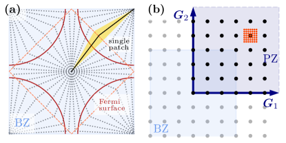
Figure 2: Meshing schemes for the functional renormalization group calculations. (a) $N$-patch meshing scheme (figure adapted from Ref. honerkamp_salmhofer_furukawa_rice ), the points are defined at the intersections of the Fermi surface (red) with the patch-lines (dashed gray). For a single patch, the yellow, filled area is projected to the same momentum point. (b) Bravais momentum mesh in primitive zone (PZ) instead of Brillouin zone (BZ) with mesh refinement around one selected point shown in orange.

The momentum resolution of the functional renormalization group is limited by two distinct issues: The lower bound is given by the ability to resolve sharp features of the fermionic momenta in the loop derivative at low scale. As these occur in the proximity of the Fermi-surface (FS) this is equivalent to demanding an accurate representation of said FS within the chosen momentum scheme. The upper bound is determined by computational limitations. Because the memory requirement for saving the vertices – the largest objects – scales proportional to $N_{\boldsymbol{k}}^{3}$, raising the fidelity of momentum discretization is constrained by availability of RAM.

The traditional method of fulfilling these two aspects is to allocate a number of points along the FS of the system to be used as momentum points for the vertex calculations [see Fig. 2 (a)]. While the vertex would only be defined on the FS, using the assumption that it is almost constant within the patch honerkamp_doping_2001 ; honerkamp_salmhofer_furukawa_rice ; N-patch-tsai , the propagators and their derivatives are evaluated for a set of points spanning the entire area of the patch. The values would be averaged to obtain the value of $\dot{L}$ at the FS patch point, finely sampling the patches area. This method is discussed in more detail in Ref. honerkamp_salmhofer_furukawa_rice .

The immediate issue with this parameterization is the evaluation of the fourth vertex momentum. Having constrained $\boldsymbol{k}_{1},\boldsymbol{k}_{2},\boldsymbol{k}_{3}$ to points on the FS we have no capacity to guarantee that $\boldsymbol{k}_{4}=\boldsymbol{k}_{1}+\boldsymbol{k}_{2}-\boldsymbol{k}_{3}$ coincides with one of the patch centers. The assumption is therefore made that this can be projected to the closest existing point, the center of the patch we land within. This method, while historically successful in the prediction of fundamental models kiesel-thomale-ea-2012 ; dlpena_scherer_honerkamp_2014 breaks momentum conservation of the interaction. This is especially problematic when attempting to analyze spin-orbit-coupled (SOC) or multi-site systems where conserving momentum becomes important due to momentum-spin-locking or momentum-orbit-locking.

The easiest method to restore momentum conservation is the introduction of an equispaced (“Bravais”) mesh within the first PZ. For this case, shown in Fig. 2 (b), the addition/subtraction of any number of momentum points is assured to be a valid momentum point. The obvious issue though is that the majority of points is now far from the FS, making the resolution of the aforementioned features doubtful.

If we were able to use arbitrarily high momentum resolutions this method would yield the exact momentum integrations. It therefore is the base-case for the simulations performed in this paper and offers the easiest implementation of all two dimensional momentum space FRG alternatives. The main challenges to overcome are the memory constrains imposed by the scaling with momentum resolution and orbital degrees of freedom. To circumvent this issue we introduce an averaging similar to the one performed in the evaluation of $N$-patch as

$$\dot{L}^{ijmn}_{\pm}(\boldsymbol{l},\boldsymbol{l}^{\prime})=\sum_{\boldsymbol{l}_{f}}\dot{L}^{ijmn}_{\pm}(\boldsymbol{l}+\boldsymbol{l}_{f},\boldsymbol{l}^{\prime}\pm\boldsymbol{l}_{f}),$$ (14)

where $\boldsymbol{l}$ is taken from the normal (coarse) fermionic mesh and $\boldsymbol{l}_{f}$ is a small (refined) offset relative to this point. We choose the sign to conserve total momentum in each channel. The resulting refined grid is shown in Fig. 2 (b). Crucially, we employ the refinement only for an averaging within the calculations of the loop derivative and require no information of the vertex on the full set of refined momentum points. As in $N$-patch, we assume the interactions to be sufficiently slowly varying such that $V(\boldsymbol{k}_{1}+\boldsymbol{l}_{f},\boldsymbol{k}_{2},\boldsymbol{k}_{3})\approx V(\boldsymbol{k}_{1},\boldsymbol{k}_{2},\boldsymbol{k}_{3})$ holds. This approximation is even more reasonable here as the maximum distance from the center is greatly decreased. Some intricacies on the exact implementation of choosing $i,j,m,n$ from orbital or band space are discussed in E and are omitted here.

2.5 Truncated Unities

Building upon the presented basic implementation of grid-FRG we now expand to further approximations. The truncated unity extension to the functional renormalization group (TUFRG) is an approach to reduce the computational complexity introduced using grid-FRG while maintaining momentum conservation. Noticing the divergences introduced in the FRG flow will stem from the loop derivative, we isolate the bosonic momentum $\boldsymbol{q}$ of $\dot{L}_{\pm}(\boldsymbol{l},\pm(\boldsymbol{q}-\boldsymbol{l}))$. For each channel ($P$, $C$, $D$) in Fig. 1 we thus obtain a distinct transfer momentum:

$$\boldsymbol{q}_{P} {}=\boldsymbol{k}_{1}+\boldsymbol{k}_{2}\,,$$ (15a)

$$\boldsymbol{q}_{C/D} {}=\boldsymbol{k}_{1}-\boldsymbol{k}_{4/3}\,.$$ (15b)

The remaining weaker fermionic dependencies of vertex and loop are expanded in a (symmetrized) basis of linearly independent functions $f_{m}(\boldsymbol{k})$ – called formfactors. The choice of these functions is based on the construction of basis functions for irreducible representations described in Ref. platt-hanke-thomale-2013 with a few improvements and generalizations detailed in G. We project/unproject the flow equations given in Fig. 1 into/from the formfactor basis using the following operators for each channel $X\in$ $P$, $C$, $D$:

$$\begin{split}\hat{X}[\Phi_{X}]_{m,n}(\boldsymbol{q})&=\int_{\mathrm{BZ}}\!\!\mathrm{d}\boldsymbol{k}\int_{\mathrm{BZ}}\!\!\mathrm{d}\boldsymbol{k}^{\prime}\\ &{}\hskip 40.00006ptf_{m}(\boldsymbol{k})f_{n}^{*}(\boldsymbol{k}^{\prime})\Phi_{X}(\boldsymbol{q},\boldsymbol{k},\boldsymbol{k}^{\prime})\,,\\ \Phi_{X}(\boldsymbol{q},\boldsymbol{k},\boldsymbol{k}^{\prime})&\approx\sum_{m,n}f_{m}(\boldsymbol{k})f_{n}^{*}(\boldsymbol{k}^{\prime})\hat{X}[\Phi_{X}]_{m,n}(\boldsymbol{q})\,.\end{split}$$ (16)

It is instructive to note that with a complete basis of formfactors this is an exact unitary transformation, but in our case we truncate the basis by neglecting long-range formfactors. This is reasonable because the interaction strength declines at long ranges LichtensteinPHD-2018 . The truncation makes the truncated unity expansion an approximation to the grid-FRG implementation, but significantly reduces the memory requirements for the vertices which shrink by a factor of $(N_{f}/N_{\boldsymbol{k}})^{2}$. This method has been developed in Ref. LichtensteinPHD-2018 based on the earlier work in Ref. wang-frg-graphene-2012 and has proven successful for Hubbard and graphene type models LichtensteinPHD-2018 ; korea_graphene_2019 ; o_competing_2021 ; dlpena_lichtenstein_honerkamp2017 .

When considering the vertex in band space, the gauge phases carried by the orbital-to-band matrices can not be disregarded. Thus, the band space vertex cannot be captured accurately in the truncated unity projections, this approximation thus necessitates orbital space calculations. TUFRG also has slight symmetry breaking at long coupling ranges for multi-site models, the details and workaround of this are described in F.

2.6 Real Space Truncated Unities

In models with broken translational symmetry, momentum is not good quantum number and we thus require a different approach to treat these systems. The proposal here is to use the real space equivalents of formfactors, which we will refer to as bonds for the sake of clarity. In real space the bosonic momentum dependence of each channel is translated to a dependence on two orbitals (or sites). The fermionic momenta are then equivalent to the remaining orbital dependencies. We define the real space bonds $g_{\boldsymbol{b}_{i}}(\boldsymbol{r}_{j})$ as Kronecker deltas spanning the lattice

$$g_{\boldsymbol{b}_{i}}(\boldsymbol{r}_{j})=\delta({\boldsymbol{r}_{i}+\boldsymbol{b}_{i},\boldsymbol{r}_{j}})\,,$$ (17)

where $\boldsymbol{r}_{i}$ is the position of the site $i$ and $\boldsymbol{b}_{i}$ is a connection to another site starting at site $i$. In the case of large unit cells, where momentum is still conserved, it may also be beneficial to introduce real space truncated unities. The projections in this mixed space representation then follow Eqs. 18a, 18b and 18c:

$$\hat{P}[V]^{o_{1}o_{3}}_{\boldsymbol{b}_{1}\boldsymbol{b}_{3}}(\boldsymbol{q}_{P})=g_{\boldsymbol{b}_{1}}(o_{2},\boldsymbol{k}_{1})g^{*}_{\boldsymbol{b}_{3}}(o_{4},\boldsymbol{k}_{3})\\ V^{o_{1}o_{2}o_{3}o_{4}}(\boldsymbol{k}_{1},\boldsymbol{q}_{P}-\boldsymbol{k}_{1};\boldsymbol{k}_{3})\,,$$ (18a)

$$\hat{C}[V]^{o_{1}o_{3}}_{\boldsymbol{b}_{1}\boldsymbol{b}_{3}}(\boldsymbol{q}_{C})=g_{\boldsymbol{b}_{1}}(o_{4},\boldsymbol{k}_{1})g^{*}_{\boldsymbol{b}_{3}}(o_{2},\boldsymbol{k}_{3})\\ V^{o_{1}o_{2}o_{3}o_{4}}(\boldsymbol{k}_{1},\boldsymbol{k}_{1}-\boldsymbol{q}_{C};\boldsymbol{k}_{3})\,,$$ (18b)

$$\hat{D}[V]^{o_{1}o_{4}}_{\boldsymbol{b}_{1}\boldsymbol{b}_{4}}(\boldsymbol{q}_{D})=g_{\boldsymbol{b}_{1}}(o_{3},\boldsymbol{k}_{1})g^{*}_{\boldsymbol{b}_{4}}(o_{2},\boldsymbol{k}_{4})\\ V^{o_{1}o_{2}o_{3}o_{4}}(\boldsymbol{k}_{1},\boldsymbol{k}_{4}-\boldsymbol{q}_{D};\boldsymbol{k}_{1}-\boldsymbol{q}_{D})\,.$$ (18c)

The generation of the sets of real space bonds and momentum space formfactors can now be performed following one of two different rules: For the first, simpler one, we assume that the two sets have no connection, allowing for a two step projection with separate real- and momentum space unities. This decouples the implementations but comes with a severe drawback: For models with more than a single site per unit cell, it is impossible to include the same interaction orders for each site, thus breaking the rotational and inversion symmetries as detailed in F. The second approach remedies these concerns by first creating all real space bonds on the full lattice with $n_{l_{1}}\cdot n_{k_{1}}\times n_{l_{2}}\cdot n_{k_{2}}$ elements, where $n_{l_{i}}$ is the number of real space unit cells and $n_{k_{i}}$ is the number of momentum points in the direction of basis vector $i$. Afterwards we perform a Fourier transform of all bonds and obtain formfactor-bonds of the following general form

$$g_{\boldsymbol{b}_{i}}(\boldsymbol{o}_{j},\boldsymbol{k}) =e^{-i\boldsymbol{k}\boldsymbol{B}_{\boldsymbol{b}_{i}}}\delta(\boldsymbol{r}_{i}+\boldsymbol{b}_{i},\boldsymbol{r}_{j})\,,$$ (19)

where $\boldsymbol{B}_{\boldsymbol{b}_{i}}$ is the beyond unit cell part of the bond $\boldsymbol{b}_{i}$. The real space TU was first developed for one dimensional systems starting from an analysis of the perturbative orders bauer-functional-2014 ; weidinger-bauer-vondelft-2017 ; markhof_detecting_2018 and was thereafter re-derived for arbitrary dimension in the context of truncated unities as we present it here in-prep-hauck .

3 Implementations

Having explained the theoretical backdrop for the implementations we now want to discuss the three distinct FRG codes independently developed by the authors, sharing minor details of the code-base (input routines, output routines). Each of the programs will be given a short introduction to establish the functionalities it covers, its merits and the contrast to the other implementations.

3.1 Code #1: grid-FRG

As the generation of band structures from ab initio simulations is common practice, it is advantageous to be able to use these as starting point for FRG calculations. Thus, this code implements the static four-point FRG equations in either band or orbital space and on a regular momentum grid and allows the study of correlation effects of arbitrary periodic systems if the following can be provided:

• A few isolated low-energy bands of the material in momentum space on a regular, fine momentum mesh.

• Addition and subtraction rules for the momentum mesh.

• The $4$-point vertex in any basis that can be connected to the band basis by unitary transformation (and thus is of the same dimension). As $V$ may be an object of large size, it is possible to supply it on a coarse momentum mesh.

• The orbital to band transform [Bloch functions $u^{ob}(\boldsymbol{k})$] for all momentum points. In case the $4$-point vertex is given in band space, the matrices fulfill $\hat{u}(\boldsymbol{k})\equiv\mathds{1}$.

Since the code is designed to operate on very general models defined only by the points given above, it is capable of running FRG simulations from e.g. Density Functional Theory (DFT) or tight-binding (TB) datasets. The latter can be generated from within the code, with appropriate skeletons given to make usage simple and efficient. Furthermore the users are enabled to employ their own, custom momentum space meshings and thus can in principle use the code for conventional $N$-patch FRG simulations – even in the multi-orbital scenario. We facilitate this by inclusion of an appropriate code skeleton.

The main computational challenge faced by this FRG implementation is memory size and bandwidth. The message passing interface (MPI) allows the vertex to be distributed on a large number of cluster nodes (with the restriction that splitting constrained to the bosonic momentum index $\boldsymbol{q}_{D}$). This code is memory-bound; simulating e.g. a six band model on a $24\times 24$ coarse momentum mesh would take $288$ compute nodes requiring $\sim 140\,\mathrm{GiB}$ memory on each node to store the vertex objects. For fewer band models these requirements are drastically lowered and allow for quick and robust operation.

3.2 Code #2: TUFRG

The aim of the TUFRG implementation is to allow fast creation and testing of new material representations. This is enabled by removing unnecessary constraints imposed in the creation of previous frameworks, generalizing the implementation as much as possible, while extending to include SOC and multi-orbital systems. The cost introduced by this inclusion has necessitated a focus on performance, while the decision to generalize for all systems has necessitated some performance hits.

Due to the generalized nature of this implementation it will be worse in large unit cells compared to Code #3 and will be slower than Code #1 for grid-FRG. It is however an extremely accessible version of FRG and should be both easily usable and adaptable to uncharted problems. Furthermore it struggles much less under the memory constraining the calculations in Code #1, a similar calculation as described above would need a single compute node, MPI is required only for calculation speed.

The framework needs as input a tight-binding model with dispersion and interaction defined in momentum space as well as a momentum basis. From this the entirety of the formfactor expansion and TUFRG calculation will be performed. As the truncated unities are based heavily on grid-FRG the framework also provides a basic implementation of grid-FRG. While this framework is capable of doing the here published grid-FRG simulations, its primary aspiration is the TUFRG.

3.3 Code #3: RS-TUFRG

The objective of this implementation is to provide a flexible and easy to use real- and mixed space TUFRG algorithm. It is optimized for large unit cells, i.e. between $10$ and a few $1000$ sites per unit cell which allows for the study of many interesting phenomena, such as edge properties, disorder effects, behavior in quasicrystalline models and effects of different boundary conditions. The models also do not have to be defined on a lattice so that structures such as Barabasi-Albért networks can be analyzed. This broad application range of course leads to slight performance deterioration, thus it is advisable to resort to Code #1 or Code #2, for small unit cells or few band problems. By including all formfactor-bonds, this code can effectively perform the grid-RG calculations presented here.

The code itself is designed to be easily extendable with user defined models. For this it requires at least a definition of the underlying lattice or graph, a tight binding Hamiltonian, and a distance measure. It also allows for the inclusion of a single Matsubara frequency per channel during the flow. This enables the scaling test, where we check for the correct error scaling behavior of the interaction when compared to exact diagonalization, as shown in H.

4 Results – Connecting to previous publications

4.1 Reproducibility: The Hubbard Model

To bolster confidence in the correctness of our results we first reproduce some established results of functional renormalization group calculations. The most basic model – thoroughly analyzed in Refs. honerkamp-salmhofer-2001 ; honerkamp_doping_2001 ; honerkamp_salmhofer_furukawa_rice ; honerkamp2003 ; honerkamp_interaction_2004 ; honerkamp_ferromagnetism_2004 ; salmhofer_renormalization_2004 ; husesalm ; Uebelacker-2021-sffeedback ; husemann_frequency_2012 ; LichtensteinPHD-2018 ; tagliavini-ea-2019-multiloop ; hille-ea-2020-quantitative ; hille_pseudogap_2020 ; bonetti_single_2021 ; schaefer-wentzell-multi-2021 – is the Hubbard model for cuprates on a two-dimensional square lattice. We reproduce the results from Refs. honerkamp-salmhofer-2001 ; LichtensteinPHD-2018 , the next-nearest-neighbor hopping phase scan of the repulsive Hubbard model at the van Hove singularity. Note that the critical scale $\Lambda_{\mathrm{c}}$, which is derived from the artificial scale parameter $\Lambda$, is associated with the temperature of the phase transition and thus corresponds to a physical observable. Throughout this section, we therefore effectively compare both the critical temperature and the type of ordering to previous literature results.

Figure 3: Square lattice Hubbard model reference results. The plots show the critical scale as a function of next-nearest-neighbor hopping $t^{\prime}$ with the chemical potential fixed at $\mu=-4t^{\prime}$ to pin the Fermi level to the van Hove singularity. Additionally, the type of instability is encoded as markers; circles: antiferromagnetism, plus signs: $d$-wave superconductivity, triangles: ferromagnetism. The interaction strength is set to $U=3$. (a) Match of the non-TU results of Codes #1 and #2 to Ref. honerkamp-salmhofer-2001 . (b) TUFRG results from Codes #2 and #3 matched to the results presented in Ref. LichtensteinPHD-2018 . It should be noted that due to differing details of approximations and simulations we do not expect the results to exactly coincide. The discrepancies are pronounced in the proximity of the transition from superconducting to ferromagnetic phase at $t^{\prime}\approx-0.35$. This region is both very dependent on implementational details as well as hard to properly resolve due to the low scales required (see B for the minimal scale allowed by our momentum resolution). This was already noted in the referred publications but is compounded by the different grid discretization chosen in (a) (grid-FRG vs N-Patch) leading to the behavior shown.

The non-interacting part of the $t-t^{\prime}$ Hubbard Hamiltonian is given by:

$$H_{0}=-\sum_{ij,\sigma}t_{ij}\,c_{i,\sigma}^{\dagger}c_{j,\sigma}^{\phantom{\dagger}}\,,$$ (20)

where the hopping amplitudes are $t_{\braket{i,j}}=1$ if $i,j$ are nearest neighbors and $t_{\braket{\braket{i,j}}}=t^{\prime}$ where $i,j$ are next-nearest neighbors. We fix the chemical potential to $\mu=-4t^{\prime}$ pinning the system to van Hove filling. The interacting part of the Hamiltonian is governed by

$$H_{\mathrm{I}}=U\,\sum_{i,\sigma}\,n_{i,\sigma}n_{i,\bar{\sigma}}\,.$$ (21)

where $n_{i,\sigma}=c^{\dagger}_{i,\sigma}c^{\phantom{\dagger}}_{i,\sigma}$. Figure 3 demonstrates how all three codes presented in this work reproduce literature in terms of both the critical scales and the type of instability (details on the analysis of the effective vertex at the critical scale are presented in C). Note that our numerical implementations differ from each other and the reference in terms of the specifics and methods chosen within the scope of grid-FRG and TUFRG. To name examples, the type of integrator, cutoff scheme, stopping scale and termination criterion were not explicitly coordinated. We observe that the value of $\Lambda_{\mathrm{c}}$ and the type of instability close to a phase transition are sensitive to these minor details, but overall the data shows agreement. The unattainable equivalence in Fig. 3 is a motivation for the exact comparison given in Section 5.

4.2 Non-$SU(2)$ Systems: The Rashba Model

To confirm all three codes’ capabilities extend beyond the $SU(2)$ symmetric one-band Hubbard model, we introduce a Rashba-$z$ spin-orbit coupling (SOC) term to the kinetic part of the Hamiltonian breaking the $SU(2)$ symmetry. It then reads

$$H_{0}=-\sum_{ij,\sigma}t_{ij}\,c_{i,\sigma}^{\dagger}c_{j,\sigma}^{\phantom{\dagger}}\,-i\alpha\sum_{\braket{ij},\sigma\sigma^{\prime}}\big{(}\hat{\boldsymbol{\sigma}}\times\boldsymbol{b}_{ij}\big{)}_{z}^{\sigma\sigma^{\prime}}c^{\dagger}_{i,\sigma}c^{\phantom{\dagger}}_{j,\sigma^{\prime}}\,,$$ (22)

where $\alpha$ is the SOC strength, $\hat{\boldsymbol{\sigma}}$ is the vector of Pauli matrices, $\braket{ij}$ denote nearest neighbors and $\boldsymbol{b}_{ij}$ are the corresponding directed bonds. Extensive coverage of Rashba-$z$ SOC in the square lattice Hubbard model will be provided by a publication in preparation in-prep-rashba where we employ FRG and the weak coupling renormalization group wolf-2020-rashba ; in-prep-schwemmer . Here we indicate only the results of a filling phase scan at fixed $\alpha=0.1,t^{\prime}=-0.15$ and $U=3$ in Fig. 4 (a) to demonstrate internal consistency.

Figure 4: Rashba and graphene model reference results. The plots show the critical scale as a function of filling factor. Markers encode the type of ordering; circles: antiferromagnetism, plus signs: $d$-wave superconductivity. (a) Rashba model. The complete analysis can be found in Ref. in-prep-rashba , here we only show internal consistency between the three implementations. We use the following parameters: $t^{\prime}=0.15$, $\alpha=0.1$, $U=3$ and the filling factor $\nu\in[0.35,0.59]$ with $\nu=0$ ($\nu=1$) corresponding to a completely empty (filled) system. (b) Graphene model. The markers and colors follow the same scheme as in (a). We choose the same parameter set as in Ref. wang-frg-graphene-2012 : $t^{\prime}=0.1$, $U=3.6$. For ease of comparison we use the doping $\delta=2\nu-1$ instead of the filling factor. The transition from magnetic to superconducting phase occurs at slightly different temperatures than in the reference which however employs singular mode FRG. Graphene is also notoriously resolution dependent (momenta and formfactors) in FRG calculations due to incommensurate phases o_competing_2021 and the multi-site nature of the system. We nonetheless obtain the central results of the publication at $\delta\approx 1/4$ as well as the transition on either side.

4.3 Multi-band Systems: Graphene

The third class of models we can check consistent results for are multi-site unit cell models. Ref. wang-frg-graphene-2012 provides singular mode FRG results for a tight-binding Hamiltonian of graphene to which we compare the three codes. The non-interacting part defined on the honeycomb lattice reads

$$H_{0}=\sum_{ij,oo^{\prime},\sigma}t_{ij,oo^{\prime}}\,c^{\dagger}_{i,o,\sigma}c^{\phantom{\dagger}}_{j,o^{\prime},\sigma}\,,$$ (23)

where $o,o^{\prime}$ are the sites within a unit cell, $i,j$ are unit cell indices and $t_{ij,oo^{\prime}}$ the hopping parameters. We set $t_{ij,oo^{\prime}}=1$ for nearest-neighbors and $t_{ij,oo^{\prime}}=t^{\prime}$ for next-nearest-neighbors. For the reproduction of the results in Fig. 4 (b) we choose $t^{\prime}=0.1$. The site-dependent Hubbard interaction with $U=3.6$ reads

$$H_{\mathrm{I}}=U\sum_{i,o,\sigma}\,n_{i,o,\sigma}n_{i,o,\bar{\sigma}}\,.$$ (24)

Additionally to the results in Fig. 4 (b), we have reproduced the critical interaction strength of the half-filled system ($\nu=0.5$) without next-nearest-neighbor hopping ($t^{\prime}=0$) to be $U_{\mathrm{crit}}\approx 2.7t$. This is in agreement with both Ref. SnchezdelaPea:754628 as well as the expectation that FRG lies between mean-field $U_{\mathrm{crit}}\approx 2.2t$ Sorella_1992 and quantum Monte-Carlo $U_{\mathrm{crit}}=3.6t-4.0t$ doi:10.1143/JPSJ.70.1483 ; paiva-qmc-2005 ; meng-2010-quantum ; sorella_absence_2012 predictions.

5 Results – Benchmark Systems

The test systems were chosen to cover a breadth of different aspects of functional renormalization group calculations in an attempt to reveal common errors. The two dimensional square lattice Hubbard model is chosen as the starting point. We choose the $SU(2)$ symmetric representation which warrants the usage of the $SU(2)$ symmetric set of flow equations from Fig. 1. To also cover the non-$SU(2)$ flow equations it is imperative to include a non-$SU(2)$ symmetric model. We therefore also consider the square-lattice Rashba model with spin-orbit coupling. While this pair of models should complete the verification of the momentum dependencies in the contractions calculated during the flow, we want to extend the benchmarks to include a multi-band model with non-orthogonal lattice vectors. This is crucial in finding phase-errors as well as non-periodicities of the Hamiltonian. We therefore evaluate and publish data for a honeycomb lattice Hubbard model, which is a simple model for graphene. While this is obviously not a complete list of possible models one could show equivalence for, inconsistencies in this subset should uncover most inconsistencies that can arise during the implementation of the FRG. If more models are desirable or advisable the equivalence class will be extended and the repository data updated appropriately.

5.1 Square lattice $SU(2)$: The Hubbard Model

The simplest test case is the square-lattice Hubbard model. Having indicated that our codes reproduce previously published results we now define parameters sets for the benchmarks. The chosen way of integration is grid-FRG – this allows the greatest confirmation across the three codes – other reproduction of data are available for comparisons upon request. Be mindful that RS-TUFRG or TUFRG benchmarks can only be supported by a subset of implementations.

Model:

To make the test as accessible as possible we shall fix $t=1$, this allows implementations which use this – rather common – scale to implement a comparative calculation. The remaining parameters of Eqs. 20 and 21 are (arbitrarily) defined to the following nonzero values: $U=3.0$ and $t^{\prime}=-0.1$. In the case of the single band $SU(2)$ symmetric Hubbard model the interaction is constant:

$$V(\boldsymbol{k}_{1},\boldsymbol{k}_{2},\boldsymbol{k}_{3})=U\,.$$ (25)

The chemical potential is defined as $\mu=0.5$. We chose to define the chemical potential rather than the filling to remove the indirection of its calculation. This process is inaccurate, especially at the small system sizes discussed here. As the first step of any momentum space FRG calculation likely is checking for correctness in the non-interacting part of the Hamiltonian, we provide band structures along the high-symmetry paths for each of the models discussed in A.

Meshing:

It is essential for exact numerical accuracy that the momentum space is meshed identically. We propose the following patching scheme: An equispaced grid of $6$ points along each edge is laid within the first PZ to include all high-symmetry-points. 36 is a sensible choice for the total number of points because while being small enough to be quickly calculated it still contains points that are not high-symmetry points. The resulting mesh can be seen in Fig. 5 (a). This mesh is used wherever momenta are needed, for the discretization of the vertex as well as the integration over the loop momentum. It should be noted that the refinement mentioned in Section 2.4 is not applied in these calculations to reduce sources of potential error.

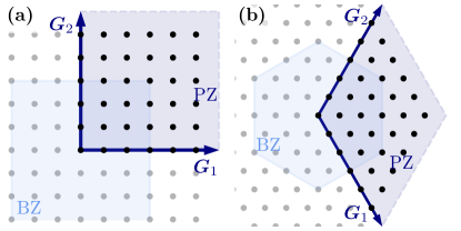
Figure 5: Momentum space meshing in test cases. (a) Square lattice models (Hubbard and Rashba) have a square Brillouin zone (BZ) and a square primitive zone (PZ) (b) Triagonal lattice systems (e.g. graphene) have a hexagonal BZ and a PZ in rhombus shape. Both meshes are an equispaced grid along the basis vectors of the reciprocal lattices $\boldsymbol{G}_{1}$ and $\boldsymbol{G}_{2}$. In the hexagonal case we can see that the PZ mesh will fill the BZ only after backfolding of points, this is intended behavior.

Flow:

The most difficult aspect of the calculations to align are the parameters and calculations involving the integration from high to low scale. There are many options of integrators, Euler or adaptive, each with a significantly different update scheme for $\mathrm{d}/\mathrm{d}\Lambda$. Even minute details such as the order of operations (calculating $\Delta_{\Lambda}(\Lambda_{n+1})$ or $\Delta_{\Lambda}(\Lambda_{n})$) are relevant. For this reason we decide to use the simplest possible integrator, constraining the issues in the numerical analysis:

The integration scheme is a fixed-stepwidth Euler integration which yields $V(\Lambda_{n+1})=V(\Lambda_{n})+\Delta_{\Lambda}\frac{\mathrm{d}V}{\mathrm{d}\Lambda}(\Lambda_{n})$. We fix $\Delta_{\Lambda}=0.1\equiv\mathrm{const.}$ and perform 90 iterations of the FRG-flow starting at $\Lambda=10$. We disable all other termination conditions and are thus certain to obtain $V(\Lambda=1.0)$. To avoid misinterpretation, we provide pseudocode for the procedure:

Algorithm 1 Flow scheme with constant update

1:$\Lambda=10$

2:$\Delta=0.1$

3:Initialize vertex $V=V_{0}$

4:for $n=0,1,\ldots,90$ do

5:     Evaluate $\dot{L}(\Lambda)$ with Eq. 7

6:     Evaluate $\frac{\mathrm{d}V}{\mathrm{d}\Lambda}(\Lambda)$ via Fig. 1

7:     $V\leftarrow V+\Delta\frac{\mathrm{d}V}{\mathrm{d}\Lambda}$

8:     $\Lambda\leftarrow\Lambda-\Delta$

9:end for

For regulator of the FRG equations we also default to the simplest possible choice, the sharp cutoff. This is used in all subsequent calculations.

5.2 Square lattice non-$SU(2)$: The Rashba Model

The meshing of the square BZ [Fig. 5 (a)] as well as the parametrization of the $\Lambda$ integration are equivalent to the setup presented for the Hubbard model.

Model:

We choose the model parameters to ensure broken particle-hole symmetry as well as broken $SU(2)$ symmetry. The non-interacting Hamiltonian is defined by Eq. 22 while the interacting part Eq. 21 can be represented as a Hubbard interaction of electrons of opposite spins:

$$V^{\sigma_{1}\sigma_{2}\sigma_{3}\sigma_{4}}(\boldsymbol{k}_{1},\boldsymbol{k}_{2},\boldsymbol{k}_{3})=\\ U(1-\delta_{\sigma_{1}\sigma_{2}})\left[\delta_{\sigma_{1}\sigma_{3}}\delta_{\sigma_{2}\sigma_{4}}-\delta_{\sigma_{1}\sigma_{4}}\delta_{\sigma_{2}\sigma_{3}}\right]\,.$$ (26)

We set the parameters to $t^{\prime}=-0.1$, $U=3.0$, $\alpha=0.5$ and $\mu=0.2$.

5.3 Hexagonal lattice $SU(2)$: The graphene Model

For the graphene model we choose the parametrization of the FRG-flow to remain equivalent but need to redefine the BZ meshing [Fig. 5 (b)].

Model:

The parameters for the calculation of graphene are: $U=3$, $t^{\prime}=0.1$ and $\mu=0.2$. Due to the sublattice structure of graphene the choice of origin in the Fourier transforms of the Hamiltonian is relevant. This is detailed in D, here it suffices to mention that we choose the proper gauge which transforms both sites of the graphene model with respect to the origin of the unit cell. Any other choice of Fourier transform would result in an improper (non-periodic) gauge of the Hamiltonian. We specify the interaction in the orbital space of graphene to be a site-local Hubbard interaction:

$$V^{o_{1}o_{2}o_{3}o_{4}}(\boldsymbol{k}_{1},\boldsymbol{k}_{2},\boldsymbol{k}_{3})=U\delta_{o_{1},o_{2}}\delta_{o_{2},o_{3}}\delta_{o_{3},o_{4}}$$ (27)

To be precise we specify the real space lattice vectors ($\boldsymbol{a}_{i}$) and positions of the atoms within the first unit cell ($\boldsymbol{x}_{i}$):

$$\boldsymbol{a}_{1} {}=(\sqrt{3}/2,-1/2,0)^{\mathrm{T}} \boldsymbol{a}_{2} {}=(\sqrt{3}/2,1/2,0)^{\mathrm{T}}\,,$$ (28)

$$\boldsymbol{x}_{1} {}=(1/\sqrt{3},0,0)^{\mathrm{T}} \boldsymbol{x}_{2} {}=(2/\sqrt{3},0,0)^{\mathrm{T}}\,.$$ (29)

Meshing:

The meshing is defined as an equispaced grid of $6\times 6$ points along the lines defined by the two reciprocal lattice vectors $\boldsymbol{G}_{1}=(2\pi/\sqrt{3},-2\pi,0)^{\mathrm{T}}$ and $\boldsymbol{G}_{2}=(2\pi/\sqrt{3},2\pi,0)^{\mathrm{T}}$. This mesh covers the PZ [cf. Fig. 5 (b)] which is equivalent to any BZ due to the above choice of proper gauge.

Using this meshing ensures an even distribution of the weights to the momentum points during integrations. As before this mesh is used for all momenta required in the calculations.

5.4 TUFRG results

As Code #2 as well as Code #3 are capable of TUFRG calculations we are also able to generate benchmarks for this approximation. Equivalence is however much harder to achieve for TUFRG and because the target audience for the comparison is smaller the results are omitted from this publication. Upon request datasets as well as exact descriptions of the procedures involved will be provided.

5.5 The Benchmarks

5.5.1 Data Availability

The dataset is publicly available data for comparisons. Simulation codes will be made available from the corresponding authors upon reasonable request. They are expected to be made available in the near future.

5.5.2 Comparing Instructions

The comparative data includes the following aspects of the FRG evaluation:

1. The maximum contribution to $\Delta_{\Lambda}\frac{\mathrm{d}V}{\mathrm{d}\Lambda}(\Lambda)$ by each of the $P$-,$C$-, $D$-channel diagrams (or the sum of the $D$-channel diagrams for the $SU(2)$ systems)

2. The maximum vertex element after each iteration of the flow

3. The final effective vertex $V(\Lambda=1.0)$ at each discretization point of the Brillouin zone (and spin/site index for Rashba/Graphene)

The first and second set of data can be compared by calculating the corresponding values in the trial implementation. The definition of maximum used is the maximal absolute value of the complex numbers $|z|=\sqrt{\mathrm{Re}(z)^{2}+\mathrm{Im}(z)^{2}}$. Discrepancies in these offer insight into possible faults in singular channels or prefactors.

The third and most important result to compare is the effective vertex at the final scale. Here we offer an array of values (of datatype double complex). The recommended approach is to sort the reference array as well as the respective result from the trial code by some metric (i.e. $\max[\mathrm{Re}(z)]$ or $\max[\mathrm{Im}(z)]$) and compare the sorted arrays. Note that equivalence can be reached only to computational accuracy (discrepancies from the resolution of double, rounding, compiler optimizations, etc. may occur).

While it is also possible to obtain element-wise reproduction, this is dependent on the order of the discretized momentum points. Because this stems from the mesh generation scheme as well as the choice of PZ, neither of which has physical implications, we recommend subverting this dependency.

6 Conclusion and Outlook

This publication set out to rectify the missing link for internal consistency of momentum space functional renormalization group calculations. We have verified the validity of the implementations by proving agreement with established results for momentum space functional renormalization group calculations and uniformity to unprecedented levels between the three implementations. This gives us the confidence in the claim that the datasets obtained are “correct” in the scope of the specific approximation (i.e. treating only the four-point vertex in momentum space while neglecting self-energies and frequency dependencies of the vertex) of FRG. We provide these results with the intent of their continued reproduction and verification by members of the FRG community. Because the realm of tests can be as vast as the scope of FRG calculations we invite a continued investment by the community. The obvious extensions include frequency and self-energy dependent calculations. Please engage with the authors for required assistance in the reproduction.

Furthermore, the authors are currently working to combine their codes under a single, versatile “community code” with a polished, common, easy-to-use interface. While this is a major undertaking it is necessary to make the resulting code accessible to both the FRG community and the more general audience of physicists interested in many-body phenomenæ.

7 Authors contributions

Each author was the lead developer on one of the respective implementations. The authors each acknowledge the other’s contributions in the development of their code in both lines of code and discussions. All the authors were involved in the preparation of the manuscript and have contributed equally to this work.

Appendix

Appendix A Band structures

In Fig. 6, we present the bandstructures of the models from the three test cases with subtracted chemical potential. In subfigure (a), we show the band structure of the square lattice Hubbard model with $t=1$, $t^{\prime}=-0.1$ and $\mu=0.5$. In subfigure (b), we show the Rashba model as defined in Eq. (22), with $t=1$, $t^{\prime}=-0.1$, $\alpha=0.5$ and $\mu=0.2$. Finally subfigure (c) shows Graphene with $t=1$, $t^{\prime}=0.1$ and $\mu=0.2$. These datasets are identical to the benchmark cases, thus reproduction of the band structures is a good initial test.

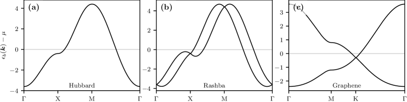
Figure 6: Band structures of (a) square lattice tight binding model (Hubbard), (b) square lattice tight binding model with Rashba-SOC (Rashba) and (c) hexagonal lattice tight binding model (graphene), where the shorthand notation associates the band structures with the benchmark systems as defined in Section 5. We note for the Hubbard model the expected saddle point at the X-point. The square lattice Rashba band structure has band crossing points at X and M while for graphene we draw attention to Dirac cone around the K-point.

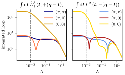
Figure 7: Integrated particle-hole (left) and particle-particle (right) loops $\int\mathrm{d}\boldsymbol{l}\,\dot{L}_{\pm}^{\Lambda}(\boldsymbol{l},\pm(\boldsymbol{q}-\boldsymbol{l}))$ at high-symmetry values of $\boldsymbol{q}$ as a function of scale $\Lambda$. The points $\boldsymbol{q}$ are indicated in the legends. Note that at $\Lambda=10^{-3}$, we add a dashed gray emphasizing the minimum value of $\Lambda$ for which the loops can be considered to be converged. Below this scale, the spacing of eigenenergies (for the discretization we chose) is larger than $\Lambda$ leading to a divergence that is cut off.

Appendix B Minimum Scale and Momentum Resolution

The oscillatory behavior at low scales seen in the critical scale as a function of $t^{\prime}$ in the grid-FRG results for the Hubbard model (see Fig. 3 (a)) implies that for $\Lambda<10^{-3}$, the momentum resolution we employed ($20\times 20$ coarse points and $25\times 25$ fine points) cannot resolve smaller scales. To support this, we show the (momentum $\boldsymbol{k}$) integrated particle-particle and particle-hole loops at high-symmetry transfer momenta as a function of $\Lambda$ obtained from the grid-FRG simulation in Fig. 7. We specifically chose the value $t^{\prime}=-0.35$ to be consistent with Fig. 3. As expected, the loops cannot be resolved to scales smaller than $\Lambda<10^{-3}$, as indicated by the dashed gray lines.

We want to further highlight the fact that these loop integrals are in fact the same as the onsite formfactor projection of the TUFRG loops. The non-oscillatory behavior of the TUFRG codes in Fig. 3 (b) as well as the small kink at around $t^{\prime}=-0.2$ can be explained by the fact that long-range interactions cannot fully be captured in TUFRG when they are present in multiple channels. Therefore, at the phase boundaries, the truncation employed leads to slightly different behavior than in the grid-FRG case – the momentum resolutions employed in the integrations are similar.

Appendix C Analysis of Effective Vertex

Having obtained the effective interaction $V^{\Lambda_{\mathrm{c}}}$ from the evaluation of the flow equations we list useful strategies to determine types of phase transitions.

Element Picking

The simplest method for phase identification is element picking. Here we consider the elements known to drive different phases and compare their values, choosing the biggest magnitude as the phase. This works very well for systems with a finite set of known and simple phases such as the Hubbard model. We can identify all three phases in Fig. 3 by means of this.

For the superconducting phase we can consider the element at $\boldsymbol{k}_{1}+\boldsymbol{k}_{2}=0$, using the remaining momentum dependencies to distinguish that we encounter a $d$-wave superconductor. In the truncated unities approximation this becomes even more powerful as the other momenta are already expanded into the formfactor basis. For the antiferromagnetic phase we consider the momentum transfer $\boldsymbol{k}_{1}-\boldsymbol{k}_{3}=(\pi,\pi)$. As this drives the $C$-channel diagram we can assume a spin-density-wave with wave vector $(\pi,\pi)$ which corresponds – on the square lattice – to antiferromagnetism. Similarly we can decipher ferromagnetism by examining the vertex at the momentum transfer $\boldsymbol{k}_{1}-\boldsymbol{k}_{3}=(0,0)$, a spin-density-wave with this wave vector corresponds to a ferromagnetic phase.

Susceptibilities

For particle-hole instabilities (spin-density waves and charge-density waves in the $SU(2)$ case), it is instructive to study the (crossed) particle-hole susceptibility using the vertex given at the end of the FRG flow projected to the corresponding channels. klebl2021moire To efficiently calculate these, we define the Fermi particle-hole loop at scale $\Lambda$ as

$$L_{f,+}^{\Lambda,o_{1}o_{2}o_{3}o_{4}}(\boldsymbol{q}_{D},\boldsymbol{k}_{D})=\sum_{b_{1}b_{2}}u^{o_{1}b_{1}}(\boldsymbol{k}^{\phantom{\prime}}_{D})u^{*o_{3}b_{1}}(\boldsymbol{k}^{\phantom{\prime}}_{D})\\ \qquad u^{o_{2}b_{2}}(\boldsymbol{k}_{D}^{\prime})u^{*o_{4}b_{2}}(\boldsymbol{k}_{D}^{\prime})\,\big{[}f\big{(}\epsilon^{\phantom{\prime}}_{D}/\Lambda\big{)}-f\big{(}\epsilon_{D}^{\prime}/\Lambda\big{)}\big{]}\\ \big{[}\epsilon^{\phantom{\prime}}_{D}-\epsilon_{D}^{\prime}\big{]}^{-1}\,,$$ (30)

with the Fermi function $f(x)=\big{(}1+e^{x}\big{)}^{-1}$ and $\epsilon^{\phantom{\prime}}_{X}=\epsilon_{b_{1}}(\boldsymbol{k}^{\phantom{\prime}}_{X}),\epsilon_{X}^{\prime}=\epsilon_{b_{2}}(\boldsymbol{k}_{X}^{\prime})$. From this, we calculate the four-point susceptibility as

$$\chi_{D}^{o_{1}o_{2}o_{3}o_{4}}(\boldsymbol{q}_{D})=\sum_{\begin{subarray}{c}\boldsymbol{k}_{D}^{\phantom{\prime}}\boldsymbol{k}_{D}^{\prime}\\ o_{1}^{\prime}o_{2}^{\prime}o_{3}^{\prime}o_{4}^{\prime}\end{subarray}}\,L_{f,+}^{\Lambda,o_{1}o_{2}o_{1}^{\prime}o_{2}^{\prime}}(\boldsymbol{q}^{\phantom{\prime}}_{D},\boldsymbol{k}^{\phantom{\prime}}_{D})\,\\ \qquad V_{D}^{\Lambda,o_{1}^{\prime}o_{2}^{\prime}o_{3}^{\prime}o_{4}^{\prime}}(\boldsymbol{q}^{\phantom{\prime}}_{D},\boldsymbol{k}^{\phantom{\prime}}_{D},\boldsymbol{k}_{D}^{\prime})\,L_{f,+}^{\Lambda,o_{3}^{\prime}o_{4}^{\prime}o_{3}o_{4}}(\boldsymbol{q}^{\phantom{\prime}}_{D},\boldsymbol{k}_{D}^{\prime})\,.$$ (31)

Linearized Gap Equation

For $P$ instabilities, it is convenient to solve a linearized gap equation to obtain details about the system’s leading ordering tendencies. klebl2021moire We define the $P$-channel Fermi loop at scale $\Lambda$ as

$$L_{f,-}^{\Lambda,o_{1}o_{2}o_{3}o_{4}}(\boldsymbol{q}_{P},\boldsymbol{k}_{P})=\sum_{b_{1}b_{2}}\,u^{o_{1}b_{1}}(\boldsymbol{k}^{\phantom{\prime}}_{P})u^{*o_{3}b_{1}}(\boldsymbol{k}^{\phantom{\prime}}_{P})\\ \qquad u^{o_{2}b_{2}}(\boldsymbol{k}^{\prime}_{P})u^{*o_{4}b_{2}}(\boldsymbol{k}^{\prime}_{P})\,\big{[}f\big{(}-\epsilon^{\phantom{\prime}}_{P}/\Lambda\big{)}-f\big{(}\epsilon_{P}^{\prime}/\Lambda\big{)}\big{]}\\ \big{[}\epsilon^{\phantom{\prime}}_{P}+\epsilon_{P}^{\prime}\big{]}^{-1}\,.$$ (32)

We can then proceed to define a superconducting linearized gap equation as

$$\lambda\,\Delta_{P}^{o_{1}o_{2}}(\boldsymbol{k})=\sum_{\boldsymbol{k}^{\prime}o_{3}o_{4}o_{1}^{\prime}o_{2}^{\prime}}V_{P}^{\Lambda,o_{1}o_{2}o_{3}o_{4}}(\boldsymbol{q}_{P}=0,\boldsymbol{k},\boldsymbol{k}^{\prime})\,\\ L_{f,\pm}^{\Lambda,o_{3}o_{4}o_{1}^{\prime}o_{2}^{\prime}}(\boldsymbol{q}_{P}=0,\boldsymbol{k}^{\prime})\,\Delta_{P}^{o_{1}^{\prime}o_{2}^{\prime}}(\boldsymbol{k}^{\prime})\,.$$ (33)

The eigenproblem in Eq. 33 is in general non-hermitian and thus numerically unstable. Therefore, we instead solve the following singular value decomposition:

$$\hat{V}_{P}^{\Lambda}\hat{L}_{f,-}^{\Lambda}=\hat{U}\,\hat{\Sigma}\,\hat{V}^{\dagger}\,.$$ (34)

The right singular vectors $\hat{V}$ are gap functions projected to the Fermi surface (with “temperature” broadening set by $\Lambda$) and the left singular vectors do not include the Fermi surface projection and display the gap’s symmetry. In the case of non-$SU(2)$ and two-site systems, it is instructive to transform the superconducting ($P$) gap to singlet [$\psi(\boldsymbol{k})$] and triplet [$\boldsymbol{d}(\boldsymbol{k})$] space sigrist1991phenomenological ; smidman2017superconductivity :

$$\hat{\Delta}(\boldsymbol{k})=i\,\big{[}\hat{\sigma}_{0}\psi(\boldsymbol{k})+\hat{\boldsymbol{\sigma}}\cdot\boldsymbol{d}(\boldsymbol{k})\big{]}\,\hat{\sigma}_{y},$$ (35)

with $\hat{\boldsymbol{\sigma}}$ Pauli matrices and $\hat{\sigma}_{0}$ the identity matrix.

Appendix D Pitfalls during evaluations

During the production of the results for each model we encountered numerous possible pitfalls which can lead to different results in the test set. The first and most important one is to make sure that the models are defined exactly as above. Other common mistakes that occur are using different sign conventions or wrong input parameters, so if the results do not match this should be the first suspect. Otherwise the following section may help identify problems in the comparison. Most of these pertain to general problems which should be taken into account when implementing an FRG-code.

Signs and prefactors of the diagrams

One of the main issues with functional renormalization group calculations is fixing the prefactors (signs and values) within the flow equations (cf. Fig. 1). Here we want to list some strategies which can be employed in order to obtain the correct values for the special case of the square lattice Hubbard model at half filling (and $t^{\prime}=0$). A graphical representation for the $SU(2)$ symmetric rules is shown in Fig. 8.

Non-$SU(2)$ diagrams

The following rules apply to the three diagrams of the non-$SU(2)$ equation:

• For an initially attractive interaction, the absolute value maximum of the $P$-channel contribution must increase over the flow (for the first steps).

• Using an initially repulsive interaction, the $C$- and $D$-channel contributions to the effective vertex must increase over the flow (for the first steps).

• The $C$- and $D$-channel contributions must be equivalent up to a reordering of the orbital and momentum indices and sign including the prefactors in the flow equations.

$SU(2)$ diagrams

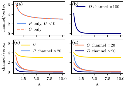
Figure 8: Graphical representation of test system properties. For all cases, we used the test system parameters, except for $\mu=0$, $t^{\prime}=0$ such that the symmetries hold. (a) Vertex maximum as a function of scale in single channel flow in $P$ for $U=-3$ (blue) and $C$ for $U=3$. The two lines are the same (point 1 in the text). (b) Full repulsive flow, $D$ channel contribution that is identically zero at first step. (cf. point 2) (c) Full repulsive flow, all channels and vertex. (cf. point 3) (d) Full attractive flow ($U=-3$) with all channels and vertex. (cf. point 4)

1. When calculating the single-channel flow in $C$- and $P$-diagrams the results must be equal when inverting $U$.

2. The total value of the $D$-channel contribution must be zero in the first step.

3. For an initially repulsive interaction, the $C$-channel contribution to the effective vertex must increase over the flow (for the first steps).

4. When calculating an attractive interaction in $P$-channel the maximum of the effective vertex must increase over the flow (for the first steps).

BZ-periodicity of systems with basis

Here we want to address the periodicity of the Hamiltonian in the case of existing sublattice structure.

Figure 9: Example lattice with sublattice structure with nearest-neighbor hopping $t$ from $B$ to $A$ site.

Fourier transforming into momentum space there are two options for handling the positions of the orbitals. We can either use the actual positions in the transformation or we map all sites onto the origin and Fourier transform with respect to this. Using the first option introduces non-periodicities. We will illustrate this using a simple two site model:

$$\begin{split}H_{0}=t\sum_{\braket{ij}}&\left(c^{\dagger}_{i,A}c^{\phantom{\dagger}}_{j,A}+c^{\dagger}_{i,B}c^{\phantom{\dagger}}_{j,B}+c^{\dagger}_{i,A}c^{\phantom{\dagger}}_{i,B}\right.\\ &\quad\left.+c^{\dagger}_{i,B}c^{\phantom{\dagger}}_{i,A}+c^{\dagger}_{i,A}c^{\phantom{\dagger}}_{j,B}+c^{\dagger}_{j,B}c^{\phantom{\dagger}}_{i,A}\right)\,.\end{split}$$ (36)

We define the Fourier transforms with respect to the origin as follows:

$$c^{\phantom{\dagger}}_{i,A}=\int_{\mathrm{BZ}}\!\!\mathrm{d}\boldsymbol{k}\,e^{i\boldsymbol{k}\boldsymbol{R}_{i}}c^{\phantom{\dagger}}_{A}$$ (37)

and

$$c^{\phantom{\dagger}}_{i,B}=\int_{\mathrm{BZ}}\!\!\mathrm{d}\boldsymbol{k}\,e^{i\boldsymbol{k}\boldsymbol{R}_{i}}c^{\phantom{\dagger}}_{B}$$ (38)

resulting in the non-interacting Hamiltonian of the form

$$H_{0}=t\int_{\mathrm{BZ}}\!\!\mathrm{d}\boldsymbol{k}\,\bigg{\{}c^{\dagger}_{A}(\boldsymbol{k})c^{\phantom{\dagger}}_{A}(\boldsymbol{k})+c^{\dagger}_{B}(\boldsymbol{k})c^{\phantom{\dagger}}_{B}(\boldsymbol{k})+c^{\dagger}_{A}(\boldsymbol{k})c^{\phantom{\dagger}}_{B}(\boldsymbol{k})\\ \qquad{}+c^{\dagger}_{B}(\boldsymbol{k})c^{\phantom{\dagger}}_{A}(\boldsymbol{k})+\sum_{\begin{subarray}{c}\boldsymbol{v}\in\{\boldsymbol{a}_{1},\boldsymbol{a}_{2},\\ \boldsymbol{a}_{1}+\boldsymbol{a}_{2}\}\end{subarray}}e^{i\boldsymbol{k}\boldsymbol{v}}\Big{[}c^{\dagger}_{A}(\boldsymbol{k})c^{\phantom{\dagger}}_{B}(\boldsymbol{k})\\ {}+c^{\dagger}_{B}(\boldsymbol{k})c^{\phantom{\dagger}}_{A}(\boldsymbol{k})\Big{]}\bigg{\}}\,,$$ (39)

which is a perfectly $2\pi$ periodic form of the non-interacting Hamiltonian. We shall call this gauge a “proper” gauge. Now to study the effects of an improper gauge, where we use the actual positioning of the sublattice within the unit cell to define the improper gauged Fourier transforms:

$$c^{\phantom{\dagger}}_{i,A}=\int_{\mathrm{BZ}}\!\!\mathrm{d}\boldsymbol{k}\,e^{i\boldsymbol{k}\boldsymbol{R}_{i}}c^{\phantom{\dagger}}_{A}$$ (40)

and

$$c^{\phantom{\dagger}}_{i,B}=\int_{\mathrm{BZ}}\!\!\mathrm{d}\boldsymbol{k}\,e^{i\boldsymbol{k}(\boldsymbol{R}_{i}+\frac{\boldsymbol{a}_{1}}{2}+\frac{\boldsymbol{a}_{2}}{2})}c^{\phantom{\dagger}}_{B}\,.$$ (41)

Using these expressions to Fourier transform $H_{0}$ we can see that we collect some phase-terms which are not $2\pi$ periodic in $\boldsymbol{k}$:

$$H_{0}=t\int_{\mathrm{BZ}}\!\!\mathrm{d}\boldsymbol{k}\,\bigg{\{}c^{\dagger}_{A}(\boldsymbol{k})c^{\phantom{\dagger}}_{A}(\boldsymbol{k})+c^{\dagger}_{B}(\boldsymbol{k})c^{\phantom{\dagger}}_{B}(\boldsymbol{k})+c^{\dagger}_{A}(\boldsymbol{k})c^{\phantom{\dagger}}_{B}(\boldsymbol{k})\\ \qquad+c^{\dagger}_{B}(\boldsymbol{k})c^{\phantom{\dagger}}_{A}(\boldsymbol{k})+\sum_{\begin{subarray}{c}\boldsymbol{v}\in\{\boldsymbol{a}_{1},\boldsymbol{a}_{2},\\ \boldsymbol{a}_{1}+\boldsymbol{a}_{2}\}\end{subarray}}e^{i\boldsymbol{k}\boldsymbol{v}}e^{i\boldsymbol{k}(\frac{\boldsymbol{a}_{1}}{2}+\frac{\boldsymbol{a}_{2}}{2})}\Big{[}c^{\dagger}_{A}(\boldsymbol{k})c^{\phantom{\dagger}}_{B}(\boldsymbol{k})\\ +c^{\dagger}_{B}(\boldsymbol{k})c^{\phantom{\dagger}}_{A}(\boldsymbol{k})\Big{]}\bigg{\}}\,.$$ (42)

We can therefore no longer evaluate $H_{0}$ after backfolding into the first BZ, instead we need to evaluate them in higher BZs.

While in theory this is a seemingly natural gauge, the periodicity of the Hamiltonian is required for the momentum meshing used in this work. Furthermore using an improper gauge will change the topological properties of the model system. The definition of a $2\pi$ periodic gauged representation is therefore of paramount importance.

Handedness of Coordinate systems

While it may be obvious we want to briefly discuss the handedness of the momentum lattice. When defining a basis of three vectors spanning space we should define the third vector such that the span product $v=(\boldsymbol{x}\times\boldsymbol{y})\cdot\boldsymbol{z}>0$. This is called a right-handed coordinate system.

When defining the real basis $\boldsymbol{a}_{i}$ of the system instead we take care that it is right handed, the momentum lattice vectors $\boldsymbol{G}_{i}$ can then be obtained via the transformations:

$$[\boldsymbol{G}_{1},\boldsymbol{G}_{2},\boldsymbol{G}_{3}]=2\pi\left([\boldsymbol{a}_{1},\boldsymbol{a}_{2},\boldsymbol{a}_{3}]^{-1}\right)^{\mathrm{T}}\,.$$ (43)

Appendix E Refinement and Symmetries

Using the refinement to subsum the dependencies within the area associated with a mesh-point we run into issues which slightly break the symmetry of the Hamiltonian. For clarity we will refer to the center the refinement collapses into as coarse point.

Definition of symmetric refinement

When defining the refined mesh points atop the coarse mesh points some attention is needed to obtain a set invariant under the symmetry operations of the coarse mesh. For an illustration of the set let us consider a hexagonal BZ into which we have introduced the coarse mesh via the methods discussed in Section 2.4. Defining the refined mesh as a scaled-down version of the coarse mesh would result in a mesh which is not invariant under the symmetry transformations, this is blatantly obvious from Fig. 10. The proper method employed in the implementations discussed here is to define a refined mesh of multiple times the size of the refined area size and reduce the points to the set which is closest to the coarse center point [Wigner-Seitz like construction, cf. Fig. 10 (b)]. Depending on the system’s lattice, it may be needed to double-count some of the refined points and introduce non-unitary integration weights.

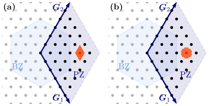
Figure 10: Refinement under symmetries. (a) Intuitive but incorrect definition of the refined mesh atop the coarse mesh. As can clearly be seen under a rotation of $C_{3}$ the indicated coarse points transform into each other, a rotation of the refinement however renders it incommensurate. (b) Proper definition of the refinement area as the Wigner-Seitz cell around the coarse point. It is apparent that these points will respect all symmetry transformations of the coarse mesh.

.

Orbital-Band-Transformation symmetry breaking

Even when using a properly symmetric refined mesh there are remaining symmetry issues in the orbital-to-band-transformations: We assume a model system with momentum-dependent orbital-orbital symmetry relations (such as the mapping of graphene-sites under rotation). When we introduce refinement we have two options of calculating the averaged non-refined loop:

• Calculate the average in band space, then transform into orbital space using the transformation matrices of the coarse points. This is subject to the band-crossing problem presented in the paragraph “Band Crossing Problem”

• Transform each refined point into orbital space and average in orbital space. This is subject to the symmetry breaking of refinement presented the paragraph “Summed Symmetries”.

Band Crossing Problem:

To illustrate the issue of evaluating the average in band space and transforming into orbital space afterwards we imagine a region of the BZ where multiple bands cross (cf. Fig. 11). Mathematically, we can formulate the problem that arises when the mapping from orbitals to bands changes as

$$\begin{split}&\sum_{\boldsymbol{k}_{f}}\sum_{b_{1}b_{2}}u^{*o_{1}b_{1}}(\boldsymbol{l}+\boldsymbol{k}_{f})u^{*o_{3}b_{2}}(\boldsymbol{l}^{\prime}\pm\boldsymbol{k}_{f})\\ &\qquad\dot{L}_{\pm}^{\Lambda,b_{1}b_{2}}(\boldsymbol{l}+\boldsymbol{k}_{f},\boldsymbol{k}-\boldsymbol{k}_{f})u^{o_{3}b_{1}}(\boldsymbol{l}+\boldsymbol{k}_{f})u^{o_{4}b_{2}}(\boldsymbol{l}\pm\boldsymbol{k}_{f})\\ &\neq\sum_{b_{1}b_{2}}u^{*o_{1}b_{1}}(\boldsymbol{l})u^{*o_{2}b_{2}}(\boldsymbol{l}^{\prime})u^{o_{3}b_{1}}(\boldsymbol{l})u^{o_{4}b_{2}}(\boldsymbol{l}^{\prime})\\ &\qquad\sum_{\boldsymbol{k}_{f}}\dot{L}^{\Lambda,b_{1}b_{2}}_{\pm}(\boldsymbol{l}+\boldsymbol{k}_{f},\boldsymbol{l}^{\prime}\pm\boldsymbol{k}_{f})\end{split}$$ (44)

Figure 11: Problem with band crossings and Refinement. When refining in band space representation the band structure shown in the left plot we ignore the fact that a band crossing occurs within the region around the coarse mesh point. The orbital-to-band transformations, calculated only at the points of the coarse mesh point will map the averaged band into the orbital space respective their order at the coarse point.

Summed Symmetries:

Applying a symmetry to the Hamiltonian reads

$$S_{\boldsymbol{k}}H(\boldsymbol{k})=U^{\dagger}(\boldsymbol{k})H(\boldsymbol{k})U(\boldsymbol{k})\,,$$ (45)

where $U$ provides the needed phase-shifts and orbital maps for the transformation of orbitals across BZ-boundaries. From this we can deduce the following relation:

$$\begin{split}S_{\boldsymbol{k}}&\Bigg{[}\sum_{\boldsymbol{k}_{f}}H(\boldsymbol{k}\pm\boldsymbol{k}_{f})\Bigg{]}\\ &=U^{\dagger}(\boldsymbol{k})\Bigg{(}\sum_{\boldsymbol{k}_{f}}H(\boldsymbol{k}\pm\boldsymbol{k}_{f})\Bigg{)}U(\boldsymbol{k})\\ &\neq\sum_{\boldsymbol{k}_{f}}U^{\dagger}(\boldsymbol{k}\pm\boldsymbol{k}_{f})H(\boldsymbol{k}\pm\boldsymbol{k}_{f})U(\boldsymbol{k}\pm\boldsymbol{k}_{f})\\ &=\sum_{\boldsymbol{k}_{f}}S_{\boldsymbol{k}\pm\boldsymbol{k}_{f}}\left[H(\boldsymbol{k}\pm\boldsymbol{k}_{f})\right]\\ &=\sum_{\boldsymbol{k}_{f}}\left[H(\boldsymbol{k}\pm\boldsymbol{k}_{f})\right]\,.\end{split}$$ (46)

Having summed over the phases of the refined points we are unable to identify the appropriate transformation matrices. This problem does not arise if the averaging is performed in band space as the phases introduced by the transformation matrices are zero – the Hamiltonian in band space corresponds to the energies.

One possible solution for this problem is thus averaging in band space (averaging the energy) and then applying the orbital-to-band transformation of the coarse point. Fortunately there exists an orbital-space solution to properly correct for these quantitative effects in the loop derivative, presented below.

Re-symmetrizing the refined loops from orbital space

Given a multi-site tight-binding system described by hopping amplitudes as a function of site indices, the matrix $U_{S}(\boldsymbol{k})$ can analytically be constructed for each point-group symmetry $S$ of the system. Note that the real space unit cell must be chosen such that its origin aligns with the system’s rotational symmetries. Otherwise, rotations (and other point-group symmetries) are only symmetries of the system with additional real space displacements (i.e. momentum-space complex phase shifts). The procedure to obtain the matrix $U_{S}(\boldsymbol{k})$ is straightforward and shortly presented in the following:

1. For each site index $o$ of the tight-binding Hamiltonian apply the symmetry $S$ to its real space position $\boldsymbol{r}_{o}$ by calculating $\tilde{\boldsymbol{r}}_{o}=\hat{S}\boldsymbol{r}_{o}$.

2. Find the site index $o^{\prime}$ and integer vector $\vec{\imath}$ (of dimension ‘dimensionality’ $D$) such that $\boldsymbol{r}_{o^{\prime}}=\vec{\imath}\cdot\vec{\boldsymbol{R}}+\tilde{\boldsymbol{r}}_{o}$ with $\vec{\boldsymbol{R}}=(\boldsymbol{R}_{1},\dots,\boldsymbol{R}_{D})^{\mathrm{T}}$ the system’s lattice vectors.

3. Save above information in a map $\boldsymbol{X}_{S}(o)$ that takes the site index $o$ and returns the vector $\boldsymbol{X}_{S}(o)$ with $\boldsymbol{X}_{S}^{1}(o)=o^{\prime}$, $\boldsymbol{X}_{S}^{2,\dots,D+1}(o)=\vec{\imath}$.

4. Set the elements of the transformation matrix to $U_{S}^{o,\boldsymbol{X}^{1}(o)}(\boldsymbol{k})=\exp\bigg{[}i\hat{S}\boldsymbol{k}\cdot\big{(}\sum_{l=1}^{D}\boldsymbol{X}^{1+l}(o)\boldsymbol{R}_{l}\big{)}\bigg{]}$.

As (free) Green’s functions transform in the same way as the tight-binding Hamiltonian under symmetries, we have

$$S\big{[}G(\boldsymbol{k})\big{]}=U^{\dagger}_{S}(\boldsymbol{k})G(\hat{S}(\boldsymbol{k}))U_{S}(\boldsymbol{k}).$$ (47)

From this, we can follow that the loops must transform as two Green’s functions in their respective orbital and momentum indices. For both the particle-particle and particle-hole loops, this amounts to

$$S\big{[}L^{o_{1}o_{2}o_{3}o_{4}}_{\pm}(\boldsymbol{k}_{1},\boldsymbol{k}_{2})\big{]}=\sum_{o_{1}^{\prime}o_{2}^{\prime}o_{3}^{\prime}o_{4}^{\prime}}U_{S}^{*,o_{1}o_{1}^{\prime}}(\boldsymbol{k}_{1})U_{S}^{o_{3}o_{3}^{\prime}}(\boldsymbol{k}_{1})\\ U_{S}^{*,o_{2}o_{2}^{\prime}}(\boldsymbol{k}_{2})U_{S}^{o_{4}o_{4}^{\prime}}(\boldsymbol{k}_{2})L^{o_{1}^{\prime}o_{2}^{\prime}o_{3}^{\prime}o_{4}^{\prime}}_{\pm}(\hat{S}\boldsymbol{k}_{1},\hat{S}\boldsymbol{k}_{2})\,.$$ (48)

Above equation holds if the site indices $o_{1}$ and $o_{3}$ correspond to one Green’s function and $o_{2}$ and $o_{4}$ to the other, with $o_{1},o_{2}$ being ingoing and $o_{3},o_{4}$ outgoing legs.

With above transformation rule at hand, we can derive a straightforward formula used for re-symmetrizing the refined loop. Let the system’s symmetry be described by a point group $\mathcal{G}$ of order $N_{\mathcal{G}}$. The re-symmetrized refined loop $L^{\mathcal{S}}$ follows as

$$L^{\mathcal{S},o_{1}o_{2}o_{3}o_{4}}_{\pm}(\boldsymbol{k}_{1},\boldsymbol{k}_{2})=\frac{1}{N_{\mathcal{G}}}\sum_{S\in\mathcal{G}}S\big{[}L^{o_{1}o_{2}o_{3}o_{4}}_{\pm}(\boldsymbol{k}_{1},\boldsymbol{k}_{2})\big{]}\,.$$ (49)

Appendix F Multi-site TUFRG and symmetries

Figure 12: Example of symmetry breaking in TUFRG. Here we want to show the symmetry breaking introduced in TUFRG when analyzing a lattice with basis. The red boxes represent the unit cells of the lattice. We consider the nearest-neighbor interaction from a B to an A site as an example. (a) Square lattice with basis in the proper gauge representation. The formfactor expansion of the nearest-neighbor onsite interaction will consist of the indicated couplings. (b) Physical representation of the couplings indicated in (a). It is apparent that this mixes different length scales and no longer respects the symmetry of the lattice.

When using the TUFRG approximation for multi-site systems we need to be aware that we introduce a mixing of differing length scales in the interaction. This is exemplified in Fig. 12 where we can clearly see that the proper-gauge representation of the interaction (all sites Fourier-transformed with respect to the same position) allows the definition of the formfactor basis only with respect to the remaining A positions. The realspace representation of the first shell is drawn in Fig. 12 (a), where we also indicate an exemplary interaction from a B-site to all neighboring A-sites. If we now transform into the physical picture in (b) we can clearly see that the seemingly consistent interaction length mixes differing length scales. If we transformed into the formfactor basis the different length scales would have been integrated into the same formfactor shell, loosing the ability to differentiate their contributions. In the cross-channel projections this introduces a slight symmetry breaking into the approximation. We see breaking of otherwise degenerate states as well as slight modifications of critical scales.

This behavior can be rectified by introducing a site-dependent formfactor expansion. We need to define a different set of neighboring formfactors for the A and B site in the above example.

Appendix G Formfactor generation

We want to detail the generalization of the formfactor generation method described in Appendix 3 of Ref. platt-hanke-thomale-2013 . In order to do this we first recall the methodology of that publication before expanding to our new approach.

Original Method

Given a symmetry Group $\mathcal{G}$ of the problem with group elements $g$ and representations $\Gamma_{i}$ with characters $\chi_{i}(g)$ we define the projectors

$$\mathcal{P}(\Gamma_{i})=\sum_{g\in\mathcal{G}}\chi_{i}^{*}(g)g,$$ (50)

into the representation’s contribution.

To now find the shell-basis for this representation apply the projector to a trial bond taken from the shell $n$ of the realspace lattice $\phi_{n}(\boldsymbol{r})=\delta_{i,i+\boldsymbol{r}}$. The result is the realspace-representation of the formfactor:

$$\varphi^{(n)}_{i}(\boldsymbol{r})=P(\Gamma_{i})\phi^{(n)}(\boldsymbol{r})=\sum_{g\in\mathcal{G}}\chi_{i}^{*}(g)g\,\phi^{(n)}_{j}(\boldsymbol{r})\,,$$ (51)

a simple Fourier transformation yields the desired momentum space formfactors:

$$\varphi_{f}(\boldsymbol{k}) {}=\sum_{\boldsymbol{r}\in\mathrm{Bonds}}e^{-i\boldsymbol{k}\cdot\boldsymbol{r}}\varphi_{f}(\boldsymbol{r})\,,$$ (52)

$$\varphi_{f}(\boldsymbol{r}) {}=\int_{\mathrm{BZ}}\!\!\mathrm{d}\boldsymbol{k}\,e^{i\boldsymbol{k}\cdot\boldsymbol{r}}\varphi_{f}(\boldsymbol{k})\,.$$ (53)

For the multi-dimensional representation we use a number of different trial bonds equal to the dimensionality. This is supposed to ensure that the number of formfactors is always sufficient to provide a unitary transformation from a realspace lattice shell into formfactor space. This however breaks down at longer ranges as will be seen in the next section.

Improved Version

The issues with the above mentioned method arise from its non-generality, the dimensionality of the representations is given but we encounter momentum shells which have more points than we have representations in the symmetry group (the fourth shell of the square lattice is an example). For these shells the above mentioned procedure does not generate a sufficient number of formfactors for the unitary transformation of the spaces. For these we are able to find multiple symmetry-inequivalent formfactors for a given representation. To produce these formfactors while maintaining orthogonality between the formfactors we use the following procedure:

For all bonds of a given length in the realspace lattice we apply the projector defined above for all representations. We reduce the obtained (too large) set of realspace formfactors $\varphi(\boldsymbol{r})$ to a linearly independent subset and orthogonalize using the Gram Schmidt orthogonalization procedure.

We can then promise the following equations for the formfactor basis:

$$\delta(\boldsymbol{k}-\boldsymbol{k}^{\prime}) {}=\sum_{f}\varphi_{f}(\boldsymbol{k})\varphi^{*}_{f}(\boldsymbol{k}^{\prime})\,,$$ (54)

$$\delta_{f,f^{\prime}} {}=\int_{\mathrm{BZ}}\!\!\mathrm{d}\boldsymbol{k}\,\varphi_{f}(\boldsymbol{k})\varphi_{f^{\prime}}(\boldsymbol{k})\,.$$ (55)

To ensure we generate the physical set of formfactors (the ones described in Ref. platt-hanke-thomale-2013 ) we use the following iterative algorithm for the generation of formfactors, this favors the formfactors generated by the original method.

Algorithm 2 Generate all formfactors of shell $n$

1:$F(n)=\emptyset$

2:while $N_{\varphi}(n)<N_{\mathrm{Bond}}(n)$ do

3:     for $\boldsymbol{b}\in n$ do

4:         for $\Gamma_{i}\in\mathcal{G}$ do

5:              $\varphi(\boldsymbol{r})=\mathcal{P}(\Gamma_{i})\boldsymbol{b}$

6:              if $\varphi(\boldsymbol{r})\neq 0$ and $a\varphi(\boldsymbol{r})\not\in F(n)\forall a\in\mathbb{C}$ then

7:                  $F=F\cap\mathcal{F}[\varphi(\boldsymbol{r})]$;

8:              end if

9:         end for

10:     end for

11:end while

The number of formfactors which need to be chosen is highly dependent upon the problem under scrutiny. If the interactions are highly localized, a few formfactors will suffice to capture the primary dependencies. A more detailed analysis of the necessary number of formfactors should be performed for each simulation.

Appendix H Scaling tests

Beyond the equivalence checks and reproduction of known results, we further checked the correct scaling behavior of our implementations against exact solutions for small systems. Therefore a short exact diagonalization code for a 1D Hubbard chain, a 1D Rashba chain and 2D graphene has been implemented. We then calculated the occupation number $\rho_{i,j}=\langle c_{i}^{\dagger}c_{j}\rangle$ using ED and a RS-TUFRG implementation in the single frequency approximation weidinger-bauer-vondelft-2017 ; reckling-honerkamp-2018 . The error is expected to scale proportionally to $U^{3}$. To verify the correct scaling behavior, roughly $60$ bosonic frequencies were necessary and the accepted error of the adaptive integrator has been set to $10^{-6}$, which allows us to verify the proportionality down to an absolute error of $\approx 10^{-6}$.

The results are summarized in Fig. 13. At low values of the interaction, the integration error leads to a deviation from the expected scaling, as can be seen in all three cases. For larger U, higher order terms can become important also deteriorating the scaling, this can be seen especially in the two 1D systems. Apart from these minor effects, the data follow the $U^{3}$-curve very closely.

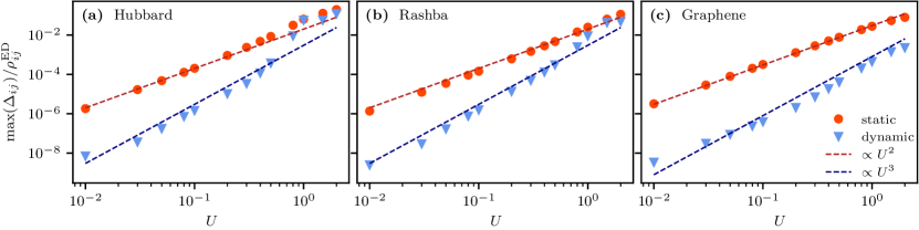
Figure 13: Scaling error of the occupation matrix compared to exact diagonalization We show the maximal error of the occupation number relative to the value of the exact diagonalization occupation number on the y-axis on a logarithmic scale. On the x-axis we show the interaction value on a logarithmic scale. As a guideline for the eye, we show the $U^{2}$ and $U^{3}$ error scalings expected from perturbative arguments. For the static calculations the error is expected to scale $\propto U^{2}$ and for the dynamic to scale $\propto U^{3}$.

References

- (1) D.S. de la Peña, J. Lichtenstein, C. Honerkamp, Phys. Rev. B 95, 085143 (2017). DOI 10.1103/PhysRevB.95.085143. URL https://link.aps.org/doi/10.1103/PhysRevB.95.085143
- (2) D.S. de la Peña, J. Lichtenstein, C. Honerkamp, M.M. Scherer, Physical Review B 96(20) (2017). DOI 10.1103/physrevb.96.205155. URL http://dx.doi.org/10.1103/PhysRevB.96.205155
- (3) S.J. O, Y.H. Kim, O.G. Pak, K.H. Jong, C.W. Ri, H.C. Pak, Physical Review B 103(23), 235150 (2021). DOI 10.1103/PhysRevB.103.235150. URL http://arxiv.org/abs/2012.05497. ArXiv: 2012.05497
- (4) S.J. O, Y.H. Kim, H.Y. Rim, H.C. Pak, S.J. Im, Phys. Rev. B 99, 245140 (2019). DOI 10.1103/PhysRevB.99.245140. URL https://link.aps.org/doi/10.1103/PhysRevB.99.245140
- (5) L. Klebl, D.M. Kennes, C. Honerkamp, Physical Review B 102(8) (2020). DOI 10.1103/physrevb.102.085109. URL http://dx.doi.org/10.1103/PhysRevB.102.085109
- (6) J.B. Hauck, C. Honerkamp, S. Achilles, D.M. Kennes, Physical Review Research 3(2) (2021). DOI 10.1103/physrevresearch.3.023180. URL http://dx.doi.org/10.1103/PhysRevResearch.3.023180
- (7) L. Classen, C. Honerkamp, M.M. Scherer, Physical Review B 99(19) (2019). DOI 10.1103/physrevb.99.195120. URL http://dx.doi.org/10.1103/PhysRevB.99.195120
- (8) M.L. Kiesel, C. Platt, W. Hanke, D.A. Abanin, R. Thomale, Physical Review B 86(2) (2012). DOI 10.1103/physrevb.86.020507. URL http://dx.doi.org/10.1103/PhysRevB.86.020507
- (9) W.S. Wang, Y.Y. Xiang, Q.H. Wang, F. Wang, F. Yang, D.H. Lee, Phys. Rev. B 85, 035414 (2012). DOI 10.1103/PhysRevB.85.035414. URL https://link.aps.org/doi/10.1103/PhysRevB.85.035414
- (10) D.S. de la Peña, M.M. Scherer, C. Honerkamp, Annalen der Physik 526(9-10), 366 (2014). DOI https://doi.org/10.1002/andp.201400088. URL https://onlinelibrary.wiley.com/doi/abs/10.1002/andp.201400088
- (11) L. Classen, M.M. Scherer, C. Honerkamp, Physical Review B 90(3) (2014). DOI 10.1103/physrevb.90.035122. URL http://dx.doi.org/10.1103/PhysRevB.90.035122
- (12) D.M. Kennes, J. Lischner, C. Karrasch, Physical Review B 98(24), 241407 (2018)
- (13) C. Honerkamp, Phys. Rev. Lett. 100, 146404 (2008). DOI 10.1103/PhysRevLett.100.146404. URL https://link.aps.org/doi/10.1103/PhysRevLett.100.146404
- (14) S. Raghu, X.L. Qi, C. Honerkamp, S.C. Zhang, Phys. Rev. Lett. 100, 156401 (2008). DOI 10.1103/PhysRevLett.100.156401. URL https://link.aps.org/doi/10.1103/PhysRevLett.100.156401
- (15) F. Wang, H. Zhai, Y. Ran, A. Vishwanath, D.H. Lee, Phys. Rev. Lett. 102, 047005 (2009). DOI 10.1103/PhysRevLett.102.047005. URL https://link.aps.org/doi/10.1103/PhysRevLett.102.047005
- (16) S. Wolf, D.D. Sante, T. Schwemmer, R. Thomale, S. Rachel. Triplet superconductivity from non-local coulomb repulsion in sn/si(111) (2021)
- (17) W. Metzner, M. Salmhofer, C. Honerkamp, V. Meden, K. Schönhammer, Rev. Mod. Phys. 84, 299 (2012). DOI 10.1103/RevModPhys.84.299. URL https://link.aps.org/doi/10.1103/RevModPhys.84.299
- (18) A. Tagliavini, C. Hille, F. Kugler, S. Andergassen, A. Toschi, C. Honerkamp, SciPost Physics 6(1), 009 (2019)
- (19) C. Hille, F.B. Kugler, C.J. Eckhardt, Y.Y. He, A. Kauch, C. Honerkamp, A. Toschi, S. Andergassen, Physical Review Research 2(3), 033372 (2020)
- (20) J. Lichtenstein, D.S.d.l. Peña, D. Rohe, E.D. Napoli, C. Honerkamp, S.A. Maier, Computer Physics Communications 213, 100 (2017). DOI https://doi.org/10.1016/j.cpc.2016.12.013. URL http://www.sciencedirect.com/science/article/pii/S0010465516303927
- (21) N. Dupuis, L. Canet, A. Eichhorn, W. Metzner, J. Pawlowski, M. Tissier, N. Wschebor, Physics Reports 910, 1–114 (2021). DOI 10.1016/j.physrep.2021.01.001. URL http://dx.doi.org/10.1016/j.physrep.2021.01.001
- (22) C. Wetterich, Physics Letters B 301(1), 90–94 (1993). DOI 10.1016/0370-2693(93)90726-x. URL http://dx.doi.org/10.1016/0370-2693(93)90726-X
- (23) T.R. MORRIS, International Journal of Modern Physics A 09(14), 2411–2449 (1994). DOI 10.1142/s0217751x94000972. URL http://dx.doi.org/10.1142/S0217751X94000972
- (24) M. Salmhofer, C. Honerkamp, Progress of Theoretical Physics 105(1), 1 (2001)
- (25) C. Honerkamp, M. Salmhofer, Phys. Rev. B 67, 174504 (2003). DOI 10.1103/PhysRevB.67.174504. URL https://link.aps.org/doi/10.1103/PhysRevB.67.174504
- (26) D. Vilardi, C. Taranto, W. Metzner, Phys. Rev. B 96, 235110 (2017). DOI 10.1103/PhysRevB.96.235110. URL https://link.aps.org/doi/10.1103/PhysRevB.96.235110
- (27) T. Reckling, C. Honerkamp, Physical Review B 98(8), 085114 (2018). DOI 10.1103/PhysRevB.98.085114. URL http://arxiv.org/abs/1803.08431. ArXiv: 1803.08431
- (28) S. Uebelacker, C. Honerkamp, Physical Review B 86(23) (2012). DOI 10.1103/physrevb.86.235140. URL http://dx.doi.org/10.1103/PhysRevB.86.235140
- (29) P.M. Bonetti, A. Toschi, C. Hille, S. Andergassen, D. Vilardi, arXiv:2105.11749 [cond-mat] (2021). URL http://arxiv.org/abs/2105.11749. ArXiv: 2105.11749
- (30) C. Honerkamp, M. Salmhofer, Phys. Rev. B 64, 184516 (2001). DOI 10.1103/PhysRevB.64.184516. URL https://link.aps.org/doi/10.1103/PhysRevB.64.184516
- (31) F.B. Kugler, J. von Delft, Physical review letters 120(5), 057403 (2018)
- (32) F.B. Kugler, J. von Delft, Physical Review B 97(3), 035162 (2018)
- (33) C.J. Eckhardt, C. Honerkamp, K. Held, A. Kauch, Physical Review B 101(15), 155104 (2020). DOI 10.1103/PhysRevB.101.155104. URL http://arxiv.org/abs/1912.07469
- (34) C. Husemann, M. Salmhofer, Physical Review B 79(19), 195125 (2009)
- (35) C. Honerkamp, M. Salmhofer, N. Furukawa, T.M. Rice, Phys. Rev. B 63, 035109 (2001). DOI 10.1103/PhysRevB.63.035109. URL https://link.aps.org/doi/10.1103/PhysRevB.63.035109
- (36) Honerkamp, C., Eur. Phys. J. B 21(1), 81 (2001). DOI 10.1007/PL00011117. URL https://doi.org/10.1007/PL00011117
- (37) L. Mathey, S.W. Tsai, A.H.C. Neto, Physical Review Letters 97(3) (2006). DOI 10.1103/physrevlett.97.030601. URL http://dx.doi.org/10.1103/PhysRevLett.97.030601
- (38) C. Platt, W. Hanke, R. Thomale, Advances in Physics 62(4-6), 453 (2013). DOI 10.1080/00018732.2013.862020. URL http://arxiv.org/abs/1310.6191. ArXiv: 1310.6191
- (39) J. Lichtenstein, Functional renormalization group studies on competing orders in the square lattice. Dissertation, RWTH Aachen University, Aachen (2018). DOI 10.18154/RWTH-2018-225781. URL https://publications.rwth-aachen.de/record/728603. Published on the publications server of the RWTH Aachen University; Dissertation, RWTH Aachen University, 2018
- (40) F. Bauer, J. Heyder, J. von Delft, Physical Review B 89(4), 045128 (2014). DOI 10.1103/PhysRevB.89.045128. URL https://link.aps.org/doi/10.1103/PhysRevB.89.045128
- (41) L. Weidinger, F. Bauer, J. von Delft, Physical Review B 95(3), 035122 (2017). DOI 10.1103/PhysRevB.95.035122. URL http://arxiv.org/abs/1609.07423. ArXiv: 1609.07423
- (42) L. Markhof, B. Sbierski, V. Meden, C. Karrasch, Physical Review B 97(23), 235126 (2018). DOI 10.1103/PhysRevB.97.235126. URL http://arxiv.org/abs/1803.00272
- (43) J.B. Hauck, D.M. Kennes, in preparation (2022)
- (44) C. Honerkamp, D. Rohe, S. Andergassen, T. Enss, Physical Review B 70(23), 235115 (2004). DOI 10.1103/PhysRevB.70.235115. URL http://arxiv.org/abs/cond-mat/0403633
- (45) C. Honerkamp, M. Salmhofer, Physica C: Superconductivity 408-410, 302 (2004). DOI 10.1016/j.physc.2004.02.089. URL http://arxiv.org/abs/cond-mat/0307541. ArXiv: cond-mat/0307541
- (46) M. Salmhofer, C. Honerkamp, W. Metzner, O. Lauscher, Progress of Theoretical Physics 112(6), 943 (2004). DOI 10.1143/PTP.112.943. URL http://arxiv.org/abs/cond-mat/0409725. ArXiv: cond-mat/0409725
- (47) C. Husemann, K.U. Giering, M. Salmhofer, Physical Review B 85(7), 075121 (2012). DOI 10.1103/PhysRevB.85.075121. URL http://arxiv.org/abs/1111.6802. ArXiv: 1111.6802
- (48) C. Hille, D. Rohe, C. Honerkamp, S. Andergassen, Physical Review Research 2(3), 033068 (2020). DOI 10.1103/PhysRevResearch.2.033068. URL http://arxiv.org/abs/2003.01447. ArXiv: 2003.01447
- (49) T. Schäfer, N. Wentzell, F. Šimkovic, Y.Y. He, C. Hille, M. Klett, C.J. Eckhardt, B. Arzhang, V. Harkov, F.m.c.M. Le Régent, A. Kirsch, Y. Wang, A.J. Kim, E. Kozik, E.A. Stepanov, A. Kauch, S. Andergassen, P. Hansmann, D. Rohe, Y.M. Vilk, J.P.F. LeBlanc, S. Zhang, A.M.S. Tremblay, M. Ferrero, O. Parcollet, A. Georges, Phys. Rev. X 11, 011058 (2021). DOI 10.1103/PhysRevX.11.011058. URL https://link.aps.org/doi/10.1103/PhysRevX.11.011058
- (50) J. Beyer, J.B. Hauck, L. Klebl, T. Schwemmer, S. Rachel, D.M. Kennes, R. Thomale, in preparation (2022)
- (51) S. Wolf, S. Rachel, Physical Review B 102(17) (2020). DOI 10.1103/physrevb.102.174512. URL http://dx.doi.org/10.1103/PhysRevB.102.174512
- (52) M. Duerrnagel, J. Beyer, R. Thomale, T. Schwemmer, in preparation (2022)
- (53) D. Sánchez de la Peña, Competing orders in honeycomb Hubbard models with nonlocal Coulomb interactions : a functional renormalization group approach. Dissertation, RWTH Aachen University, Aachen (2018). DOI 10.18154/RWTH-2019-01283. URL https://publications.rwth-aachen.de/record/754628. Veröffentlicht auf dem Publikationsserver der RWTH Aachen University 2019; Dissertation, RWTH Aachen University, 2018
- (54) S. Sorella, E. Tosatti, Europhysics Letters (EPL) 19(8), 699 (1992). DOI 10.1209/0295-5075/19/8/007. URL https://doi.org/10.1209/0295-5075/19/8/007
- (55) N. Furukawa, Journal of the Physical Society of Japan 70(6), 1483 (2001). DOI 10.1143/JPSJ.70.1483. URL https://doi.org/10.1143/JPSJ.70.1483
- (56) T. Paiva, R.T. Scalettar, W. Zheng, R.R.P. Singh, J. Oitmaa, Physical Review B 72(8) (2005). DOI 10.1103/physrevb.72.085123. URL http://dx.doi.org/10.1103/PhysRevB.72.085123
- (57) Z.Y. Meng, T.C. Lang, S. Wessel, F.F. Assaad, A. Muramatsu, Nature 464(7290), 847–851 (2010). DOI 10.1038/nature08942. URL http://dx.doi.org/10.1038/nature08942
- (58) S. Sorella, Y. Otsuka, S. Yunoki, Scientific Reports 2(1), 992 (2012). DOI 10.1038/srep00992. URL http://www.nature.com/articles/srep00992
- (59) Data for ”reference results for the momentum space functional renormalization group” (2022). DOI 10.5281/zenodo.5848606. URL https://zenodo.org/record/5848606
- (60) L. Klebl, Q. Xu, A. Fischer, L. Xian, M. Claassen, A. Rubio, D.M. Kennes, Electronic Structure (2022). URL http://iopscience.iop.org/article/10.1088/2516-1075/ac49f5
- (61) M. Sigrist, K. Ueda, Rev. Mod. Phys. 63, 239 (1991). DOI 10.1103/RevModPhys.63.239. URL https://link.aps.org/doi/10.1103/RevModPhys.63.239
- (62) M. Smidman, M.B. Salamon, H.Q. Yuan, D.F. Agterberg, Reports on Progress in Physics 80(3), 036501 (2017). DOI 10.1088/1361-6633/80/3/036501. URL https://doi.org/10.1088/1361-6633/80/3/036501