Uniform Inference for Kernel Density Estimators with Dyadic Data

Abstract

Dyadic data is often encountered when quantities of interest are associated with the edges of a network. As such it plays an important role in statistics, econometrics and many other data science disciplines. We consider the problem of uniformly estimating a dyadic Lebesgue density function, focusing on nonparametric kernel-based estimators taking the form of dyadic empirical processes. Our main contributions include the minimax-optimal uniform convergence rate of the dyadic kernel density estimator, along with strong approximation results for the associated standardized and Studentized $t$-processes. A consistent variance estimator enables the construction of valid and feasible uniform confidence bands for the unknown density function. We showcase the broad applicability of our results by developing novel counterfactual density estimation and inference methodology for dyadic data, which can be used for causal inference and program evaluation. A crucial feature of dyadic distributions is that they may be “degenerate” at certain points in the support of the data, a property making our analysis somewhat delicate. Nonetheless our methods for uniform inference remain robust to the potential presence of such points. For implementation purposes, we discuss inference procedures based on positive semi-definite covariance estimators, mean squared error optimal bandwidth selectors and robust bias correction techniques. We illustrate the empirical finite-sample performance of our methods both in simulations and with real-world trade data, for which we make comparisons between observed and counterfactual trade distributions in different years. Our technical results concerning strong approximations and maximal inequalities are of potential independent interest.

Keywords: dyadic data, networks, kernel density estimation, minimaxity, strong approximation, counterfactual analysis.

1 Introduction

Dyadic data, also known as graphon data, plays an important role in the statistical, social, behavioral and biomedical sciences. In network settings, this type of dependent data captures interactions between the units of study, and its analysis is of interest in statistics (Kolaczyk,, 2009), economics (Graham,, 2020), psychology (Kenny et al.,, 2020), public health (Luke and Harris,, 2007) and many other data science disciplines. For $n\geq 2$, a dyadic data set contains $\frac{1}{2}n(n-1)$ observed real-valued random variables

$$\mathbf{W}_{n}=(W_{ij}:1\leq i<j\leq n),\quad\qquad W_{ij} =W(A_{i},A_{j},V_{ij}),$$

where $W$ is an unknown function, $\mathbf{A}_{n}=(A_{i}:1\leq i\leq n)$ are independent and identically distributed (i.i.d.) latent random variables, and $\mathbf{V}_{n}=(V_{ij}:1\leq i<j\leq n)$ are i.i.d. latent random variables independent of $\mathbf{A}_{n}$. A natural interpretation of this data is as a complete undirected network on $n$ vertices, with the latent variable $A_{i}$ associated with node $i$ and the observed variable $W_{ij}$ associated with the edge between nodes $i$ and $j$. The data generating process above is justified without loss of generality by the celebrated Aldous–Hoover representation theorem for exchangeable arrays (Aldous,, 1981; Hoover,, 1979).

Various distributional features of dyadic data are of interest in applications. Most of the statistical literature focuses on parametric analysis, almost exclusively considering moments of (transformations of) the identically distributed $W_{ij}$. See Davezies et al., (2021), Gao and Ma, (2021), Matsushita and Otsu, (2021), and references therein, for contemporary contributions and overviews. More recently, however, a few nonparametric procedures for dyadic data have been proposed in the literature (Graham et al.,, 2021, 2023).

With the aim of estimating density-like functions associated with $W_{ij}$ using nonparametric kernel-based methods, we investigate the statistical properties of a class of local stochastic processes given by

$$w\mapsto\widehat{f}_{W}(w)=\frac{2}{n(n-1)}\sum_{i=1}^{n-1}\sum_{j=i+1}^{n}k_{h}(W_{ij},w),$$ (1)

where $k_{h}(\cdot,w)$ is a kernel function that can change with the $n$-varying bandwidth parameter $h=h(n)$ and the evaluation point $w\in\mathcal{W}\subseteq\mathbb{R}$. For each $w\in\mathcal{W}$ and with an appropriate choice of the kernel function (e.g. $k_{h}(\cdot,w)=K((\cdot-w)/h)/h$ for an interior point $w$ of $\mathcal{W}$ and a fixed symmetric integrable kernel function $K$), the statistic $\widehat{f}_{W}(w)$ becomes a kernel density estimator for the Lebesgue density function $f_{W}(w)=\mathbb{E}\big{[}f_{W\mid AA}(w\mid A_{i},A_{j})\big{]}$, where $f_{W\mid AA}(w\mid A_{i},A_{j})$ denotes the conditional Lebesgue density of $W_{ij}$ given $A_{i}$ and $A_{j}$. Setting $k_{h}(\cdot,w)=K((\cdot-w)/h)/h$, Graham et al., (2023) recently introduced the dyadic point estimator $\widehat{f}_{W}(w)$ and studied its large sample properties pointwise in $w\in\mathcal{W}=\mathbb{R}$, while Chiang and Tan, (2023) established its rate of convergence uniformly in $w\in\mathcal{W}$ for a compact interval $\mathcal{W}$ strictly contained in the support of the dyadic data $W_{ij}$. Chiang et al., (2023) obtained a distributional approximation for the supremum statistic $\sup_{w\in\mathcal{W}}\big{|}\widehat{f}_{W}(w)\big{|}$ over a finite collection $\mathcal{W}$ of design points. More generally, as we discuss below, the estimand $f_{W}(w)$ is useful in different applications because it forms the basis for counterfactual distributional analysis (Section 7) and other nonparametric and semiparametric methods (Section 8). We remark that while we assume throughout that the network is complete, our approach generalizes in a straightforward way to networks with missing edges, as in Section 7.1. This can be seen by setting $W_{ij}=-\infty$ whenever the edge $\{i,j\}$ is not present, so that the law of $W_{ij}$ is a mixture between a continuous distribution and a point mass at $-\infty$. We then apply our methodology to recover the continuous component of this distribution, following Chiang et al., (2023).

We contribute to the emerging literature on nonparametric smoothing methods for dyadic data with two main technical results. Firstly, we derive the minimax rate of uniform convergence for density estimation with dyadic data and show that the estimator $\widehat{f}_{W}$ in (1) is minimax-optimal under appropriate conditions. Secondly, we present a set of uniform distributional approximation results for the entire stochastic process $\big{(}\widehat{f}_{W}(w):w\in\mathcal{W}\big{)}$. Furthermore, we illustrate the usefulness of our main results with two distinct substantive statistical applications: (i) confidence bands for $f_{W}$ (Section 5), and (ii) estimation and inference for counterfactual dyadic distributions (Section 7). Our main results also lay the foundation for studying the uniform distributional properties of other nonparametric and semiparametric tests and estimators based on dyadic data (Section 8). Importantly, our inference results cannot be deduced from the existing U-statistic, empirical process and U-process theory available in the literature (van der Vaart and Wellner,, 1996; Giné and Nickl,, 2021) because, as explained in detail below, $\widehat{f}_{W}(w)$ is not a standard U-statistic, nor is the stochastic process $\widehat{f}_{W}$ Donsker in general, and the underlying dyadic data $\mathbf{W}_{n}$ exhibits statistical dependence due to its network structure.

Section 2 outlines the setup and presents the main assumptions imposed throughout the paper. We first discuss a Hoeffding-type decomposition of the U-statistic-like $\widehat{f}_{W}$ which is more general than the standard Hoeffding decomposition for second-order U-statistics due to its dyadic data structure. In particular, (2) shows that $\widehat{f}_{W}(w)$ decomposes into a sum of the four terms $B_{n}(w)$, $L_{n}(w)$, $E_{n}(w)$ and $Q_{n}(w)$, where $E_{n}(w)$ is not present in the classical second-order U-statistic theory. The first term $B_{n}(w)$ captures the usual smoothing bias, the second term $L_{n}(w)$ is akin to the Hájek projection for second-order U-statistics, the third term $E_{n}(w)$ is a mean-zero double average of conditionally independent terms, and the fourth term $Q_{n}(w)$ is a negligible totally degenerate second-order U-process. The leading stochastic fluctuations of the process $\widehat{f}_{W}$ are captured by $L_{n}$ and $E_{n}$, both of which are known to be asymptotically distributed as Gaussian random variables pointwise in $w\in\mathcal{W}$ (Graham et al.,, 2023). However, the Hájek projection term $L_{n}$ will often be “degenerate” at some or possibly all evaluation points $w\in\mathcal{W}$.

Section 3 studies minimax convergence rates for point estimation of $f_{W}$ uniformly over $\mathcal{W}$ and gives precise conditions under which the estimator $\widehat{f}_{W}$ is minimax-optimal. Firstly, in Theorem 3.1 we establish the uniform rate of convergence of $\widehat{f}_{W}$ for $f_{W}$. This result improves upon the recent paper of Chiang and Tan, (2023) by allowing for compactly supported dyadic data and generic kernel-like functions $k_{h}$ (including boundary-adaptive kernels), while also explicitly accounting for possible degeneracy of the Hájek projection term $L_{n}$ at some or possibly all points $w\in\mathcal{W}$. Secondly, in Theorem 3.2 we derive the minimax uniform convergence rate for estimating $f_{W}$, again allowing for possible degeneracy, and verify that it is achieved by $\widehat{f}_{W}$. This result appears to be new to the literature, complementing recent work on parametric moment estimation using graphon data (Gao and Ma,, 2021) and on nonparametric kernel-based regression using dyadic data (Graham et al.,, 2021).

Section 4 presents a distributional analysis of the stochastic process $\widehat{f}_{W}$ uniformly in $w\in\mathcal{W}$. Because $\widehat{f}_{W}$ is not asymptotically tight in general, it does not converge weakly in the space of uniformly bounded real functions supported on $\mathcal{W}$ and equipped with the uniform norm (van der Vaart and Wellner,, 1996), and hence is non-Donsker. To circumvent this problem, we employ strong approximation methods to characterize its distributional properties. Up to the smoothing bias term $B_{n}$ and the negligible term $Q_{n}$, it is enough to consider the stochastic process $w\mapsto L_{n}(w)+E_{n}(w)$. Since $L_{n}$ can be degenerate at some or possibly all points $w\in\mathcal{W}$, and also because under some bandwidth choices both $L_{n}$ and $E_{n}$ can be of comparable order, it is crucial to analyze the joint distributional properties of $L_{n}$ and $E_{n}$. To do so, we employ a carefully crafted conditioning approach where we first establish an unconditional strong approximation for $L_{n}$ and a conditional-on-$\mathbf{A}_{n}$ strong approximation for $E_{n}$. We then combine these to obtain a strong approximation for $L_{n}+E_{n}$.

The stochastic process $L_{n}$ is an empirical process indexed by an $n$-varying class of functions depending only on the i.i.d. random variables $\mathbf{A}_{n}$. Thus we use the celebrated Hungarian construction (Komlós et al.,, 1975), building on ideas in Giné et al., (2004) and Giné and Nickl, (2010). The resulting rate of strong approximation is optimal, and follows from a generic strong approximation result of potential independent interest given in Section SA3 of the online supplemental appendix. Our main result for $L_{n}$ is given as Lemma 4.1, and makes explicit the potential presence of degenerate points.

The stochastic process $E_{n}$ is an empirical process depending on the dyadic variables $W_{ij}$ and indexed by an $n$-varying class of functions. When conditioning on $\mathbf{A}_{n}$, the variables $W_{ij}$ are independent but not necessarily identically distributed (i.n.i.d.), and thus we establish a conditional-on-$\mathbf{A}_{n}$ strong approximation for $E_{n}$ based on the Yurinskii coupling (Yurinskii,, 1978), leveraging a recent refinement obtained by Belloni et al., (2019, Lemma 38). This result follows from a generic strong approximation result which gives a novel rate of strong approximation for (local) empirical processes based on i.n.i.d. data, given in Section SA3 of the online supplemental appendix. Lemma 4.2 gives our conditional strong approximation for $E_{n}$.

Once the unconditional strong approximation for $L_{n}$ and the conditional-on-$\mathbf{A}_{n}$ strong approximation for $E_{n}$ are established, we show how to properly “glue” them together to deduce a final unconditional strong approximation for $L_{n}+E_{n}$ and hence also for $\widehat{f}_{W}$ and its associated $t$-process. This final step requires some additional technical work. Firstly, building on our conditional strong approximation for $E_{n}$, we establish an unconditional strong approximation for $E_{n}$ in Lemma 4.3. We then employ a generalization of the celebrated Vorob’ev–Berkes–Philipp theorem (Dudley,, 1999), given in Section SA3 of the online supplemental appendix, to deduce a joint strong approximation for $(L_{n},E_{n})$ and, in particular, for $L_{n}+E_{n}$. Thus we obtain our main result in Theorem 4.1, which establishes a valid strong approximation for $\widehat{f}_{W}$ and its associated $t$-process. This uniform inference result complements the recent contribution of Davezies et al., (2021), which is not applicable here because $\widehat{f}_{W}$ is non-Donsker in general.

We illustrate the applicability of our strong approximation result for $\widehat{f}_{W}$ and its associated $t$-process by constructing valid standardized uniform confidence bands for the unknown density function $f_{W}$. Instead of relying on extreme value theory (e.g. Giné et al.,, 2004), we employ anti-concentration methods, following Chernozhukov et al., (2014). This illustration improves on the recent work of Chiang et al., (2023), which obtained simultaneous confidence intervals for the dyadic density $f_{W}$ based on a high-dimensional central limit theorem over rectangles, following prior work by Chernozhukov et al., (2017). The distributional approximation therein is applied to the Hájek projection term $L_{n}$ only, whereas our main construction leading to Theorem 4.1 gives a strong approximation for the entire U-process-like $\widehat{f}_{W}$ and its associated $t$-process, uniformly on $\mathcal{W}$. As a consequence, our uniform inference theory is robust to potential unknown degeneracies in $L_{n}$ by virtue of our strong approximation of $L_{n}+E_{n}$ and the use of proper standardization, delivering a “rate-adaptive” inference procedure. Our result appears to be the first to provide confidence bands that are valid uniformly over $w\in\mathcal{W}$ rather than over some finite collection of design points. Moreover, they provide distributional approximations for the whole $t$-statistic process, which can be useful in applications where functionals other than the supremum are of interest.

Section 5 addresses outstanding issues of implementation. Firstly, we discuss estimation of the covariance function of the Gaussian process underlying our strong approximation results. We present two estimators, one based on the plug-in method, and the other based on a positive semi-definite regularization thereof (Laurent and Rendl,, 2005). We derive the uniform convergence rates for both estimators in Lemma 5.1, which we then use to justify Studentization of $\widehat{f}_{W}$ and a feasible simulation-based approximation of the infeasible Gaussian process underlying our strong approximation results. Secondly, we discuss integrated mean squared error (IMSE) bandwidth selection and provide a simple rule-of-thumb implementation for applications (Wand and Jones,, 1994; Simonoff,, 2012). Thirdly, we provide feasible, valid uniform inference methods for $f_{W}$ by employing robust bias correction (Calonico et al.,, 2018, 2022). Algorithm 1 summarizes our entire feasible methodology.

Section 6 reports empirical evidence for our proposed feasible robust bias-corrected confidence bands for $f_{W}$. We use simulations to show that these confidence bands are robust to potential unknown degenerate points in the underlying dyadic distribution.

Section 7 presents novel results for counterfactual dyadic density estimation and inference, offering an application of our general theory to a substantive problem in statistics and other data science disciplines. Counterfactual distributions are important for causal inference and policy evaluation (DiNardo et al.,, 1996; Chernozhukov et al.,, 2013), and in the context of network data, such analysis can be used to answer empirical questions such as “what would the international trade distribution in one year have been if the gross domestic product (GDP) of the countries had remained the same as in a previous year?” We formally show how our theory for kernel-based dyadic estimators can be used to infer the counterfactual density function of dyadic data had some monadic covariates followed a different distribution. We propose a two-step semiparametric reweighting approach in which we first estimate the Radon–Nikodym derivative between the observed and counterfactual covariate distributions using a simple parametric estimator, and then use this to construct a weighted dyadic kernel density estimator. We present uniform consistency, strong approximation and feasible inference results for this dyadic counterfactual density estimator. Finally, we also illustrate our methods with a real dyadic data set recording bilateral trade between countries, using GDP as a covariate for the counterfactual analysis.

Section 8 discusses further statistical applications of our main results, including dyadic density hypothesis testing and nonparametric and semiparametric dyadic regression. Section 9 concludes the paper. The online supplemental appendix includes other technical and methodological results, proofs and additional details omitted here to conserve space. Section SA3 may be of independent interest, containing two generic strong approximation theorems for empirical processes, a generalized Vorob’ev–Berkes–Philipp theorem and a maximal inequality for i.n.i.d. random variables.

1.1 Notation

The total variation norm of a real-valued function $g$ of a single real variable is defined to be $\|g\|_{\mathrm{TV}}=\sup_{n\geq 1}\sup_{x_{1}\leq\cdots\leq x_{n}}\sum_{i=1}^{n-1}|g(x_{i+1})-g(x_{i})|$. For an integer $m\geq 0$, denote by $\mathcal{C}^{m}(\mathcal{X})$ the space of all $m$-times continuously differentiable functions on $\mathcal{X}$. For $\beta>0$ and $C>0$, define the Hölder class on $\mathcal{X}$ to be $\mathcal{H}^{\beta}_{C}(\mathcal{X})=\big{\{}g\in\mathcal{C}^{\ThisStyle{\ensurestackMath{\stackengine{-0.5\LMpt}{\SavedStyle\beta}{\SavedStyle{\rule{3.7pt}{0.3pt}}}{U}{c}{F}{F}{S}}\vphantom{\beta}}}(\mathcal{X}):\ \max_{1\leq r\leq\ThisStyle{\ensurestackMath{\stackengine{-0.5\LMpt}{\SavedStyle\beta}{\SavedStyle{\rule{3.7pt}{0.3pt}}}{U}{c}{F}{F}{S}}\vphantom{\beta}}}\big{|}g^{(r)}(x)\big{|}\leq C\text{ and }\big{|}g^{(\ThisStyle{\ensurestackMath{\stackengine{-0.5\LMpt}{\SavedStyle\beta}{\SavedStyle{\rule{3.7pt}{0.3pt}}}{U}{c}{F}{F}{S}}\vphantom{\beta}})}(x)-g^{(\ThisStyle{\ensurestackMath{\stackengine{-0.5\LMpt}{\SavedStyle\beta}{\SavedStyle{\rule{3.7pt}{0.3pt}}}{U}{c}{F}{F}{S}}\vphantom{\beta}})}(x^{\prime})\big{|}\leq C|x-x^{\prime}|^{\beta-\ThisStyle{\ensurestackMath{\stackengine{-0.5\LMpt}{\SavedStyle\beta}{\SavedStyle{\rule{3.7pt}{0.3pt}}}{U}{c}{F}{F}{S}}\vphantom{\beta}}},\ \forall x,x^{\prime}\in\mathcal{X}\big{\}},$ where $\ThisStyle{\ensurestackMath{\stackengine{-0.5\LMpt}{\SavedStyle\beta}{\SavedStyle{\rule{3.7pt}{0.3pt}}}{U}{c}{F}{F}{S}}\vphantom{\beta}}$ denotes the largest integer which is strictly less than $\beta$. For $a\in\mathbb{R}$ and $b\geq 0$, we write $[a\pm b]$ for the interval $[a-b,a+b]$. For non-negative sequences $a_{n}$ and $b_{n}$, write $a_{n}\lesssim b_{n}$ or $a_{n}=O(b_{n})$ to indicate that $a_{n}/b_{n}$ is bounded for $n\geq 1$. Write $a_{n}\ll b_{n}$ or $a_{n}=o(b_{n})$ if $a_{n}/b_{n}\to 0$. If $a_{n}\lesssim b_{n}\lesssim a_{n}$, write $a_{n}\asymp b_{n}$. For random non-negative sequences $A_{n}$ and $B_{n}$, write $A_{n}\lesssim_{\mathbb{P}}B_{n}$ or $A_{n}=O_{\mathbb{P}}(B_{n})$ if $A_{n}/B_{n}$ is bounded in probability. Write $A_{n}=o_{\mathbb{P}}(B_{n})$ if $A_{n}/B_{n}\to 0$ in probability. For $a,b\in\mathbb{R}$, define $a\wedge b=\min\{a,b\}$ and $a\vee b=\max\{a,b\}$.

2 Setup

We impose the following two assumptions throughout this paper.

Assumption 2.1 (Data generation)

Let $\mathbf{A}_{n}=(A_{i}:1\leq i\leq n)$ be i.i.d. random variables supported on $\mathcal{A}\subseteq\mathbb{R}$ and let $\mathbf{V}_{n}=(V_{ij}:1\leq i<j\leq n)$ be i.i.d. random variables with a Lebesgue density $f_{V}$ on $\mathbb{R}$, with $\mathbf{A}_{n}$ independent of $\mathbf{V}_{n}$. Let $W_{ij}=W(A_{i},A_{j},V_{ij})$ and $\mathbf{W}_{n}=(W_{ij}:1\leq i<j\leq n)$, where $W$ is an unknown real-valued function which is symmetric in its first two arguments. Let $\mathcal{W}\subseteq\mathbb{R}$ be a compact interval with positive Lebesgue measure $\operatorname{Leb}(\mathcal{W})$. The conditional distribution of $W_{ij}$ given $A_{i}$ and $A_{j}$ admits a Lebesgue density $f_{W\mid AA}(w\mid A_{i},A_{j})$. For $C_{\mathrm{H}}>0$ and $\beta\geq 1$, take $f_{W}\in\mathcal{H}^{\beta}_{C_{\mathrm{H}}}(\mathcal{W})$ where $f_{W}(w)=\mathbb{E}\left[f_{W\mid AA}(w\mid A_{i},A_{j})\right]$ and $f_{W\mid AA}(\cdot\mid a,a^{\prime})\in\mathcal{H}^{1}_{C_{\mathrm{H}}}(\mathcal{W})$ for all $a,a^{\prime}\in\mathcal{A}$. Suppose $\sup_{w\in\mathcal{W}}\|f_{W\mid A}(w\mid\cdot\,)\|_{\mathrm{TV}}<\infty$ where $f_{W\mid A}(w\mid a)=\mathbb{E}\left[f_{W\mid AA}(w\mid A_{i},a)\right]$.

In Assumption 2.1 we require the density $f_{W}$ be in a $\beta$-smooth Hölder class of functions on the compact interval $\mathcal{W}$. Hölder classes are well-established in the minimax estimation literature (Giné and Nickl,, 2021), with the smoothness parameter $\beta$ appearing in the minimax-optimal rate of convergence. If the Hölder condition is satisfied only piecewise, then our results remain valid provided that the boundaries between the pieces are known and treated as boundary points.

Assumption 2.2 (Kernels and bandwidth)

Let $h=h(n)>0$ be a sequence of bandwidths satisfying $h\log n\to 0$ and $\frac{\log n}{n^{2}h}\to 0$. For each $w\in\mathcal{W}$, let $k_{h}(\cdot,w)$ be a real-valued function supported on $[w\pm h]\cap\mathcal{W}$. For an integer $p\geq 1$, let $k_{h}$ belong to a family of boundary bias-corrected kernels of order $p$, i.e.,

$$\int_{\mathcal{W}}(s-w)^{r}k_{h}(s,w)\,\mathrm{d}s\quad\begin{cases}\begin{aligned} &=1&\qquad&\text{for all }w\in\mathcal{W}\text{ if }\,r=0,\\ &=0&&\text{for all }w\in\mathcal{W}\text{ if }\,1\leq r\leq p-1,\\ &\neq 0&&\text{for some }w\in\mathcal{W}\text{ if }\,r=p.\end{aligned}\end{cases}$$

Also, for $C_{\mathrm{L}}>0$, suppose $k_{h}(s,\cdot)\in\mathcal{H}^{1}_{C_{\mathrm{L}}h^{-2}}(\mathcal{W})$ for all $s\in\mathcal{W}$.

This assumption allows for all standard compactly supported and possibly boundary-corrected kernel functions (Wand and Jones,, 1994; Simonoff,, 2012). Assumption 2.2 implies that if $h\leq 1$ then $k_{h}$ is uniformly bounded by $C_{\mathrm{k}}h^{-1}$ where $C_{\mathrm{k}}\vcentcolon=2C_{\mathrm{L}}+1+1/\operatorname{Leb}(\mathcal{W})$.

2.1 Hoeffding-type decomposition and degeneracy

The estimator $\widehat{f}_{W}(w)$ is akin to a U-statistic and thus admits a Hoeffding-type decomposition which is the starting point for our analysis. We have

$$\widehat{f}_{W}(w)-f_{W}(w)=B_{n}(w)+L_{n}(w)+E_{n}(w)+Q_{n}(w)$$ (2)

with $B_{n}(w)=\mathbb{E}\big{[}\widehat{f}_{W}(w)\big{]}-f_{W}(w)$ and

$$L_{n}(w) =\frac{2}{n}\sum_{i=1}^{n}l_{i}(w), E_{n}(w) =\frac{2}{n(n-1)}\sum_{i=1}^{n-1}\sum_{j=i+1}^{n}e_{ij}(w), Q_{n}(w) =\frac{2}{n(n-1)}\sum_{i=1}^{n-1}\sum_{j=i+1}^{n}q_{ij}(w),$$

where $l_{i}(w)=\mathbb{E}[k_{h}(W_{ij},w)\mid A_{i}]-\mathbb{E}[k_{h}(W_{ij},w)]$, $e_{ij}(w)=k_{h}(W_{ij},w)-\mathbb{E}[k_{h}(W_{ij},w)\mid A_{i},A_{j}]$ and $q_{ij}(w)=\mathbb{E}[k_{h}(W_{ij},w)\mid A_{i},A_{j}]-\mathbb{E}[k_{h}(W_{ij},w)\mid A_{i}]-\mathbb{E}[k_{h}(W_{ij},w)\mid A_{j}]+\mathbb{E}[k_{h}(W_{ij},w)]$. The non-random term $B_{n}$ captures the smoothing (or misspecification) bias, while the three stochastic processes $L_{n}$, $E_{n}$ and $Q_{n}$ capture the variance of the estimator. These processes are mean-zero with $\mathbb{E}[L_{n}(w)]=\mathbb{E}[Q_{n}(w)]=\mathbb{E}[E_{n}(w)]=0$ for all $w\in\mathcal{W}$, and mutually orthogonal in $L^{2}(\mathbb{P})$ since $\mathbb{E}[L_{n}(w)Q_{n}(w^{\prime})]=\mathbb{E}[L_{n}(w)E_{n}(w^{\prime})]=\mathbb{E}[Q_{n}(w)E_{n}(w^{\prime})]=0$ for all $w,w^{\prime}\in\mathcal{W}$.

The stochastic process $L_{n}$ is akin to the Hájek projection of a U-process, which can (and often will) exhibit degeneracy at some or possibly all points $w\in\mathcal{W}$. To characterize different types of degeneracy, we introduce the following non-negative lower and upper degeneracy constants:

$$D_{\textup{lo}}^{2}:=\inf_{w\in\mathcal{W}}\operatorname{Var}\left[f_{W\mid A}(w\mid A_{i})\right]\qquad\text{ and }\qquad D_{\textup{up}}^{2}:=\sup_{w\in\mathcal{W}}\operatorname{Var}\left[f_{W\mid A}(w\mid A_{i})\right].$$

The following lemma describes the stochastic order of different terms in the Hoeffding-type decomposition, explicitly accounting for potential degeneracy.

Lemma 2.1 (Bias and variance)

Suppose that Assumptions 2.1 and 2.2 hold. Then the bias term satisfies $\sup_{w\in\mathcal{W}}\big{|}B_{n}(w)\big{|}\lesssim h^{p\wedge\beta}$ and the variance terms satisfy

$$\mathbb{E}\left[\sup_{w\in\mathcal{W}}|L_{n}(w)|\right] \lesssim\frac{D_{\textup{up}}}{\sqrt{n}}, \mathbb{E}\left[\sup_{w\in\mathcal{W}}|E_{n}(w)|\right] \lesssim\sqrt{\frac{\log n}{n^{2}h}}, \mathbb{E}\left[\sup_{w\in\mathcal{W}}|Q_{n}(w)|\right]\lesssim\frac{1}{n}.$$

Lemma 2.1 captures the potential total degeneracy of $L_{n}$ by showing that if $D_{\textup{up}}=0$ then $L_{n}=0$ everywhere on $\mathcal{W}$ almost surely. The following lemma captures the potential partial degeneracy of $L_{n}$, where $D_{\textup{up}}>D_{\textup{lo}}=0$. For $w,w^{\prime}\in\mathcal{W}$, define the covariance function of the dyadic kernel density estimator as

$$\Sigma_{n}(w,w^{\prime})=\mathbb{E}\Big{[}\Big{(}\widehat{f}_{W}(w)-\mathbb{E}\big{[}\widehat{f}_{W}(w)\big{]}\Big{)}\Big{(}\widehat{f}_{W}(w^{\prime})-\mathbb{E}\big{[}\widehat{f}_{W}(w^{\prime})\big{]}\Big{)}\Big{]}.$$

Lemma 2.2 (Variance bounds)

Suppose that Assumptions 2.1 and 2.2 hold. Then for sufficiently large $n$,

$$\frac{D_{\textup{lo}}^{2}}{n}+\frac{1}{n^{2}h}\inf_{w\in\mathcal{W}}f_{W}(w) \lesssim\inf_{w\in\mathcal{W}}\Sigma_{n}(w,w)\leq\sup_{w\in\mathcal{W}}\Sigma_{n}(w,w)\lesssim\frac{D_{\textup{up}}^{2}}{n}+\frac{1}{n^{2}h}.$$

Combining Lemmas 2.1 and 2.2, we have the following trichotomy for degeneracy of dyadic distributions based on $D_{\textup{lo}}$ and $D_{\textup{up}}$: (i) total degeneracy if $D_{\textup{up}}=D_{\textup{lo}}=0$, (ii) partial degeneracy if $D_{\textup{up}}>D_{\textup{lo}}=0$, (iii) no degeneracy if $D_{\textup{lo}}>0$. In the case of no degeneracy, it can be shown that $\inf_{w\in\mathcal{W}}\operatorname{Var}[L_{n}(w)]\gtrsim n^{-1}$, while in the case of total degeneracy, $L_{n}(w)=0$ for all $w\in\mathcal{W}$ almost surely. When the dyadic distribution is partially degenerate, there exists at least one point $w\in\mathcal{W}$ such that $\operatorname{Var}\left[f_{W\mid A}(w\mid A_{i})\right]=0$ and $\operatorname{Var}[L_{n}(w)]\lesssim hn^{-1}$, and there also exists at least one point $w^{\prime}\in\mathcal{W}$ such that $\operatorname{Var}\left[f_{W\mid A}(w^{\prime}\mid A_{i})\right]>0$ and $\operatorname{Var}[L_{n}(w^{\prime})]\gtrsim\frac{1}{n}$. We say $w$ is a degenerate point if $\operatorname{Var}\left[f_{W\mid A}(w\mid A_{i})\right]=0$, and otherwise say it is a non-degenerate point.

As a simple example, consider the family of dyadic distributions $\mathbb{P}_{\pi}$ indexed by $\pi=(\pi_{1},\pi_{2},\pi_{3})$ with $\sum_{i=1}^{3}\pi_{i}=1$ and $\pi_{i}\geq 0$, generated by $W_{ij}=A_{i}A_{j}+V_{ij}$, where $A_{i}$ equals $-1$ with probability $\pi_{1}$, equals $0$ with probability $\pi_{2}$ and equals $+1$ with probability $\pi_{3}$, and $V_{ij}$ is standard Gaussian. This model induces a latent “community structure” where community membership is determined by the value of $A_{i}$ for each node $i$, and the interaction outcome $W_{ij}$ is a function only of the communities which $i$ and $j$ belong to and some idiosyncratic noise. Unlike the stochastic block model (Kolaczyk,, 2009), our setup assumes that community membership has no impact on edge existence, as we work with fully connected networks; see Section 7.1 for a discussion of how to handle missing edges in practice. Also note that the parameter of interest in this paper is the Lebesgue density of a continuous random variable $W_{ij}$ rather than the probability of network edge existence, which is the focus of graphon estimation literature (Gao and Ma,, 2021).

In line with Assumption 2.1, $\mathbf{A}_{n}$ and $\mathbf{V}_{n}$ are i.i.d. sequences independent of each other. Then $f_{W\mid AA}(w\mid A_{i},A_{j})=\phi(w-A_{i}A_{j})$,  $f_{W\mid A}(w\mid A_{i})=\pi_{1}\phi(w+A_{i})+\pi_{2}\phi(w)+\pi_{3}\phi(w-A_{i})$ and $f_{W}(w)=(\pi_{1}^{2}+\pi_{3}^{2})\phi(w-1)+\pi_{2}(2-\pi_{2})\phi(w)+2\pi_{1}\pi_{3}\phi(w+1),$ where $\phi$ denotes the probability density function of the standard normal distribution. Note that $f_{W}(w)$ is strictly positive for all $w\in\mathbb{R}$. Consider the parameter choices:

1. $\pi=\left(\frac{1}{2},0,\frac{1}{2}\right)$: $\mathbb{P}_{\pi}$ is degenerate at all $w\in\mathbb{R}$,

2. $\pi=\left(\frac{1}{4},0,\frac{3}{4}\right)$: $\mathbb{P}_{\pi}$ is degenerate only at $w=0$,

3. $\pi=\left(\frac{1}{5},\frac{1}{5},\frac{3}{5}\right)$: $\mathbb{P}_{\pi}$ is non-degenerate for all $w\in\mathbb{R}$.

Figure 1 demonstrates these phenomena, plotting the unconditional density $f_{W}$ and the standard deviation of the conditional density $f_{W|A}$ over $\mathcal{W}=[-2,2]$ for each choice of the parameter $\pi$.

The trichotomy of total/partial/no degeneracy is useful for understanding the distributional properties of the dyadic kernel density estimator $\widehat{f}_{W}(w)$. Crucially, our need for uniformity in $w$ complicates the simpler degeneracy/no degeneracy dichotomy observed previously in the literature (Graham et al.,, 2023). More specifically, from a pointwise-in-$w$ perspective, partial degeneracy causes no issues, while it is a fundamental problem when conducting inference uniformly over $w\in\mathcal{W}$. We develop inference methods that are valid uniformly over $w\in\mathcal{W}$, regardless of the presence of partial or total degeneracy.

(a) Total degeneracy,
$\pi=\left(\frac{1}{2},0,\frac{1}{2}\right)$

(b) Partial degeneracy,
$\pi=\left(\frac{1}{4},0,\frac{3}{4}\right)$

(c) No degeneracy,
$\pi=\left(\frac{1}{5},\frac{1}{5},\frac{3}{5}\right)$

Figure 1: Density $f_{W}$ and standard deviation of $f_{W|A}$ for the family of distributions $\mathbb{P}_{\pi}$.

3 Point estimation results

Using Lemma 2.1, the next theorem establishes the uniform convergence rate of $\widehat{f}_{W}$.

Theorem 3.1 (Uniform convergence rate)

Suppose that Assumptions 2.1 and 2.2 hold. Then

$$\mathbb{E}\left[\sup_{w\in\mathcal{W}}\big{|}\widehat{f}_{W}(w)-f_{W}(w)\big{|}\right]\lesssim h^{p\wedge\beta}+\frac{D_{\textup{up}}}{\sqrt{n}}+\sqrt{\frac{\log n}{n^{2}h}}.$$

The constant in Theorem 3.1 depends only on $\mathcal{W}$, $\beta$, $C_{\mathrm{H}}$ and the choice of kernel. We interpret this result in light of the degeneracy trichotomy.

1. Partial or no degeneracy: $D_{\textup{up}}>0$. Any bandwidths satisfying $n^{-1}\log n\lesssim h\lesssim n^{-\frac{1}{2(p\wedge\beta)}}$ yield $\mathbb{E}\big{[}\sup_{w\in\mathcal{W}}\big{|}\widehat{f}_{W}(w)-f_{W}(w)\big{|}\big{]}\lesssim\frac{1}{\sqrt{n}}$, the “parametric” bandwidth-independent rate noted by Graham et al., (2023).

2. Total degeneracy: $D_{\textup{up}}=0$. Minimizing the bound in Theorem 3.1 with $h\asymp\left(\frac{\log n}{n^{2}}\right)^{\frac{1}{2(p\wedge\beta)+1}}$ yields $\mathbb{E}\big{[}\sup_{w\in\mathcal{W}}\big{|}\widehat{f}_{W}(w)-f_{W}(w)\big{|}\big{]}\lesssim\big{(}\frac{\log n}{n^{2}}\big{)}^{\frac{p\wedge\beta}{2(p\wedge\beta)+1}}$.

These results generalize Chiang and Tan, (2023, Theorem 1) by allowing for compactly supported data and more general kernel-like functions $k_{h}(\cdot,w)$, enabling boundary-adaptive density estimation.

3.1 Minimax optimality

We establish the minimax rate under the supremum norm for density estimation with dyadic data. This implies minimax optimality of the kernel density estimator $\widehat{f}_{W}$, regardless of the degeneracy type of the dyadic distribution.

Theorem 3.2 (Uniform minimax rate)

Fix $\beta\geq 1$ and $C_{\mathrm{H}}>0$, and let $\mathcal{W}$ be a compact interval with positive Lebesgue measure. Define $\mathcal{P}=\mathcal{P}(\mathcal{W},\beta,C_{\mathrm{H}})$ as the class of dyadic distributions satisfying Assumption 2.1. Define $\mathcal{P}_{\mathrm{d}}$ as the subclass of $\mathcal{P}$ containing only those dyadic distributions which are totally degenerate on $\mathcal{W}$ in the sense that $\sup_{w\in\mathcal{W}}\operatorname{Var}\left[f_{W\mid A}(w\mid A_{i})\right]=0$. Then we have $\inf_{\widetilde{f}_{W}}\sup_{\mathbb{P}\in\mathcal{P}}\mathbb{E}_{\mathbb{P}}\big{[}\sup_{w\in\mathcal{W}}\big{|}\widetilde{f}_{W}(w)-f_{W}(w)\big{|}\big{]}\asymp\frac{1}{\sqrt{n}}$ and $\inf_{\widetilde{f}_{W}}\sup_{\mathbb{P}\in\mathcal{P}_{\mathrm{d}}}\mathbb{E}_{\mathbb{P}}\big{[}\sup_{w\in\mathcal{W}}\big{|}\widetilde{f}_{W}(w)-f_{W}(w)\big{|}\big{]}\asymp\big{(}\frac{\log n}{n^{2}}\big{)}^{\frac{\beta}{2\beta+1}}$, where $\widetilde{f}_{W}$ is any estimator depending only on the data $\mathbf{W}_{n}=(W_{ij}:1\leq i<j\leq n)$ distributed according to the dyadic distribution $\mathbb{P}$. The constants underlying $\asymp$ depend only on $\mathcal{W}$, $\beta$ and $C_{\mathrm{H}}$.

Theorem 3.2 shows that the uniform convergence rate of $n^{-1/2}$ obtained in Theorem 3.1 (coming from the $L_{n}$ term) is minimax-optimal in general. When attention is restricted to totally degenerate dyadic distributions, $\widehat{f}_{W}$ also achieves the minimax rate of uniform convergence (assuming a kernel of sufficiently high order $p\geq\beta$), which is on the order of $\left(\frac{\log n}{n^{2}}\right)^{\frac{\beta}{2\beta+1}}$ and is determined by the bias $B_{n}$ and the leading variance term $E_{n}$ in (2).

Combining Theorems 3.1 and 3.2, we conclude that the estimator $\widehat{f}_{W}(w)$ achieves the minimax-optimal rate of uniform convergence for estimating $f_{W}(w)$ if $h\asymp\left(\frac{\log n}{n^{2}}\right)^{\frac{1}{2\beta+1}}$ and $p\geq\beta$, whether or not there are any degenerate points in the underlying data generating process. This result appears to be new to the literature on nonparametric estimation with dyadic data. See Gao and Ma, (2021) for a contemporaneous review.

4 Distributional results

We investigate the distributional properties of the standardized $t$-statistic process

$$T_{n}(w)=\frac{\widehat{f}_{W}(w)-f_{W}(w)}{\sqrt{\Sigma_{n}(w,w)}},\qquad w\in\mathcal{W},$$

which is not necessarily asymptotically tight. Therefore, to approximate the distribution of the entire $t$-statistic process, as well as specific functionals thereof, we rely on a novel strong approximation approach outlined in this section. Our results can be used to perform valid uniform inference irrespective of the degeneracy type.

This section is largely concerned with distributional properties and thus frequently requires copies of stochastic processes. For succinctness of notation, we will not differentiate between a process and its copy, but details are available in Section SA3 of the supplemental appendix.

4.1 Strong approximation

By the Hoeffding-type decomposition (2) and Lemma 2.1, it suffices to consider the distributional properties of the stochastic process $(L_{n}(w)+E_{n}(w):w\in\mathcal{W})$. Our approach combines the Kómlos–Major–Tusnády (KMT) approximation (Komlós et al.,, 1975) to obtain a strong approximation of $L_{n}$ with a Yurinskii approximation (Yurinskii,, 1978) to obtain a conditional (on $\mathbf{A}_{n}$) strong approximation of $E_{n}$. The latter is necessary because $E_{n}$ is akin to a local empirical process of i.n.i.d. random variables, conditional on $\mathbf{A}_{n}$, and therefore the KMT approximation is not applicable. These approximations are then combined to give a final (unconditional) strong approximation for $L_{n}+E_{n}$, and thus for the $t$-statistic process $(T_{n}(w):w\in\mathcal{W})$.

The following lemma is an application of our generic KMT approximation result for empirical processes, given in Section SA3 of the online supplemental appendix, which builds on earlier work by Giné et al., (2004) and Giné and Nickl, (2010) and may be of independent interest.

Lemma 4.1 (Strong approximation of $L_{n}$)

Suppose that Assumptions 2.1 and 2.2 hold. For each $n$ there exists a mean-zero Gaussian process $Z^{L}_{n}$ indexed on $\mathcal{W}$ satisfying $\mathbb{E}\big{[}\sup_{w\in\mathcal{W}}\big{|}\sqrt{n}L_{n}(w)-Z_{n}^{L}(w)\big{|}\big{]}\lesssim\frac{D_{\textup{up}}\log n}{\sqrt{n}}$, where $\mathbb{E}[Z_{n}^{L}(w)Z_{n}^{L}(w^{\prime})]=n\mathbb{E}[L_{n}(w)L_{n}(w^{\prime})]$ for all $w,w^{\prime}\in\mathcal{W}$. The process $Z_{n}^{L}$ is a function only of $\mathbf{A}_{n}$ and some random noise independent of $(\mathbf{A}_{n},\mathbf{V}_{n})$.

The strong approximation result in Lemma 4.1 would be sufficient to develop valid and even optimal uniform inference procedures whenever (i) $D_{\textup{lo}}>0$ (no degeneracy in $L_{n}$) and (ii) $nh\gg\log n$ ($L_{n}$ is leading). In this special case, the recent Donsker-type results of Davezies et al., (2021) can be applied to analyze the limiting distribution of the stochastic process $\widehat{f}_{W}$. Alternatively, again only when $L_{n}$ is non-degenerate and leading, standard empirical process methods could also be used. However, even in the special case when $\widehat{f}_{W}(w)$ is asymptotically Donsker, our result in Lemma 4.1 improves upon the literature by providing a rate-optimal strong approximation for $\widehat{f}_{W}$ as opposed to only a weak convergence result. See Theorem 4.2 and the subsequent discussion below.

More importantly, as illustrated above, it is common in the literature to find dyadic distributions which exhibit partial or total degeneracy, making the process $\widehat{f}_{W}$ non-Donsker. Thus approximating only $L_{n}$ is in general insufficient for valid uniform inference, and it is necessary to capture the distributional properties of $E_{n}$ as well. The following lemma is an application of our strong approximation result for empirical processes based on the Yurinskii approximation, which builds on a refinement by Belloni et al., (2019).

Lemma 4.2 (Conditional strong approximation of $E_{n}$)

Suppose Assumptions 2.1 and 2.2 hold and take any $R_{n}\to\infty$. For each $n$ there exists $\widetilde{Z}^{E}_{n}$ which is a mean-zero Gaussian process conditional on $\mathbf{A}_{n}$ satisfying $\sup_{w\in\mathcal{W}}\big{|}\sqrt{n^{2}h}E_{n}(w)-\widetilde{Z}_{n}^{E}(w)\big{|}\lesssim_{\mathbb{P}}\frac{(\log n)^{3/8}R_{n}}{n^{1/4}h^{3/8}}$, where $\mathbb{E}[\widetilde{Z}_{n}^{E}(w)\widetilde{Z}_{n}^{E}(w^{\prime})\bigm{|}\mathbf{A}_{n}]=n^{2}h\mathbb{E}[E_{n}(w)E_{n}(w^{\prime})\bigm{|}\mathbf{A}_{n}]$ for all $w,w^{\prime}\in\mathcal{W}$.

The process $\widetilde{Z}_{n}^{E}$ is a Gaussian process conditional on $\mathbf{A}_{n}$ but is not in general a Gaussian process unconditionally. The following lemma further constructs an unconditional Gaussian process $Z_{n}^{E}$ that approximates $\widetilde{Z}_{n}^{E}$.

Lemma 4.3 (Unconditional strong approximation of $E_{n}$)

Suppose that Assumptions 2.1 and 2.2 hold. For each $n$ there exists a mean-zero Gaussian process $Z^{E}_{n}$ satisfying $\mathbb{E}\big{[}\sup_{w\in\mathcal{W}}\big{|}\widetilde{Z}_{n}^{E}(w)-Z_{n}^{E}(w)\big{|}\big{]}\lesssim\frac{(\log n)^{2/3}}{n^{1/6}}$, where $Z_{n}^{E}$ is independent of $\mathbf{A}_{n}$ and $\mathbb{E}[Z_{n}^{E}(w)Z_{n}^{E}(w^{\prime})]=\mathbb{E}[\widetilde{Z}_{n}^{E}(w)\widetilde{Z}_{n}^{E}(w^{\prime})]=n^{2}h\,\mathbb{E}[E_{n}(w)E_{n}(w^{\prime})]$ for all $w,w^{\prime}\in\mathcal{W}$.

Combining Lemmas 4.2 and 4.3, we obtain an unconditional strong approximation for $E_{n}$. The resulting rate of approximation may not be optimal, due to the Yurinskii coupling, but to the best of our knowledge it is the first in the literature for the process $E_{n}$, and hence for $\widehat{f}_{W}$ and its associated $t$-process in the context of dyadic data. The approximation rate is sufficiently fast to allow for optimal bandwidth choices; see Section 5 for more details. Strong approximation results for local empirical processes (e.g. Giné and Nickl,, 2010) are not applicable here because the summands in the non-negligible $E_{n}$ are not (conditionally) i.i.d. Likewise, neither standard empirical process and U-process theory (van der Vaart and Wellner,, 1996; Giné and Nickl,, 2021) nor the recent results in Davezies et al., (2021) are applicable to the non-Donsker process $E_{n}$.

The previous lemmas showed that $L_{n}$ is $\sqrt{n}$-consistent while $E_{n}$ is $\sqrt{n^{2}h}$-consistent (pointwise in $w$), showcasing the importance of careful standardization (cf. Studentization in Section 5) for the purpose of rate adaptivity to the unknown degeneracy type. In other words, a challenge in conducting uniform inference is that the finite-dimensional distributions of the stochastic process $L_{n}+E_{n}$, and hence those of $\widehat{f}_{W}$ and its associated $t$-process $T_{n}$, may converge at different rates at different points $w\in\mathcal{W}$. The following theorem provides an (infeasible) inference procedure which is fully adaptive to such potential unknown degeneracy.

Theorem 4.1 (Strong approximation of $T_{n}$)

Suppose that Assumptions 2.1 and 2.2 hold and $f_{W}(w)>0$ on $\mathcal{W}$, and take any $R_{n}\to\infty$. Then for each $n$ there exists a centered Gaussian process $Z_{n}^{T}$ such that

$$\sup_{w\in\mathcal{W}}\left|T_{n}(w)-Z_{n}^{T}(w)\right|\lesssim_{\mathbb{P}}\frac{n^{-1}\log n+n^{-5/4}h^{-7/8}(\log n)^{3/8}R_{n}+n^{-7/6}h^{-1/2}(\log n)^{2/3}+h^{p\wedge\beta}}{D_{\textup{lo}}/\sqrt{n}+1/\sqrt{n^{2}h}},$$

where $\mathbb{E}[Z_{n}^{T}(w)Z_{n}^{T}(w^{\prime})]=\mathbb{E}[T_{n}(w)T_{n}(w^{\prime})]$ for all $w,w^{\prime}\in\mathcal{W}$.

The first term in the numerator corresponds to the strong approximation error for $L_{n}$ in Lemma 4.1 and the error introduced by $Q_{n}$. The second and third terms correspond to the conditional and unconditional strong approximation errors for $E_{n}$ in Lemmas 4.2 and 4.3, respectively. The fourth term is from the smoothing bias result in Lemma 2.1. The denominator is the lower bound on the standard deviation $\Sigma_{n}(w,w)^{1/2}$ formulated in Lemma 2.2.

In the absence of degenerate points ($D_{\textup{lo}}>0$) and if $nh^{7/2}\gtrsim 1$, Theorem 4.1 offers a strong approximation of the $t$-process at the rate $(\log n)/\sqrt{n}+\sqrt{n}h^{p\wedge\beta}$, which matches the celebrated KMT approximation rate for i.i.d. data plus the smoothing bias. Therefore, our novel $t$-process strong approximation can achieve the optimal KMT rate for non-degenerate dyadic distributions provided that $p\wedge\beta\geq 3.5$. This is achievable if a fourth-order (boundary-adaptive) kernel is used and $f_{W}$ is sufficiently smooth.

In the presence of partial or total degeneracy ($D_{\textup{lo}}=0$), Theorem 4.1 provides a strong approximation for the $t$-process at the rate $\sqrt{h}\log n+n^{-1/4}h^{-3/8}(\log n)^{3/8}R_{n}+n^{-1/6}(\log n)^{2/3}+nh^{1/2+p\wedge\beta}$. If, for example, $nh^{p\wedge\beta}\lesssim 1$, then our result can achieve a strong approximation rate of $n^{-1/7}$ up to $\log n$ terms. Theorem 4.1 appears to be the first in the dyadic literature which is also robust to the presence of (unknown) degenerate points in the underlying dyadic distribution.

4.2 Application: confidence bands

Theorem 4.2 constructs standardized confidence bands for $f_{W}$ which are infeasible as they depend on the unknown population variance $\Sigma_{n}$. In Section 5 we will make this inference procedure feasible by proposing a valid estimator of the covariance function $\Sigma_{n}$ for Studentization, as well as developing bandwidth selection and robust bias correction methods. Before presenting our result on valid infeasible uniform confidence bands, we first impose in Assumption 4.1 some extra restrictions on the bandwidth sequence, which depend on the degeneracy type of the dyadic distribution, to ensure the coverage rate converges in large samples.

Assumption 4.1 (Rate restriction for uniform confidence bands)

Assume that one of the following holds:

1. No degeneracy ($D_{\textup{lo}}>0$): $n^{-6/7}\log n\ll h\ll(n\log n)^{-\frac{1}{2(p\wedge\beta)}}$,

2. Partial or total degeneracy ($D_{\textup{lo}}=0$): $n^{-2/3}(\log n)^{7/3}\ll h\ll(n^{2}\log n)^{-\frac{1}{2(p\wedge\beta)+1}}$.

We now construct the infeasible uniform confidence bands. For $\alpha\in(0,1)$, let $q_{1-\alpha}$ be the quantile satisfying $\mathbb{P}\left(\sup_{w\in\mathcal{W}}\left|Z_{n}^{T}(w)\right|\leq q_{1-\alpha}\right)=1-\alpha$. The following result employs the anti-concentration idea due to Chernozhukov et al., (2014) to deduce valid standardized confidence bands, where we approximate the quantile of the unknown finite sample distribution of $\sup_{w\in\mathcal{W}}|T_{n}(w)|$ by the quantile $q_{1-\alpha}$ of $\sup_{w\in\mathcal{W}}|Z_{n}^{T}(w)|$. This approach offers a better rate of convergence than relying on extreme value theory for the distributional approximation, hence improving the finite sample performance of the proposed confidence bands.

Theorem 4.2 (Infeasible uniform confidence bands)

Suppose that Assumptions 2.1, 2.2 and 4.1 hold and $f_{W}(w)>0$ on $\mathcal{W}$. Then

$$\mathbb{P}\left(f_{W}(w)\in\left[\widehat{f}_{W}(w)\pm q_{1-\alpha}\sqrt{\Sigma_{n}(w,w)}\,\right]\,\textup{for all }w\in\mathcal{W}\right)\to 1-\alpha.$$

By Theorem 3.1, the asymptotically optimal choice of bandwidth for uniform convergence is $h\asymp((\log n)/n^{2})^{\frac{1}{2(p\wedge\beta)+1}}$. As discussed in the next section, the approximate IMSE-optimal bandwidth is $h\asymp(1/n^{2})^{\frac{1}{2(p\wedge\beta)+1}}$. Both bandwidth choices satisfy Assumption 4.1 only in the case of no degeneracy. The degenerate cases in Assumption 4.1(ii), which require $p\wedge\beta>1$, exhibit behavior more similar to that of standard nonparametric kernel-based estimation and so the aforementioned optimal bandwidth choices will lead to a non-negligible smoothing bias in the distributional approximation for $T_{n}$. Different approaches are available in the literature to address this issue, including undersmoothing or ignoring the bias (Hall and Kang,, 2001), bias correction (Hall,, 1992), robust bias correction (Calonico et al.,, 2018, 2022) and Lepskii’s method (Lepskii,, 1992; Birgé,, 2001), among others. In the next section we develop a feasible uniform inference procedure, based on robust bias correction methods, which amounts to first selecting an optimal bandwidth for the point estimator $\widehat{f}_{W}$ using a $p$th-order kernel, and then correcting the bias of the point estimator while also adjusting the standardization (Studentization) when forming the $t$-statistic $T_{n}$.

Importantly, regardless of the specific implementation details, Theorem 4.2 shows that any bandwidth sequence $h$ satisfying both (i) and (ii) in Assumption 4.1 leads to valid uniform inference which is robust and adaptive to the (unknown) degeneracy type.

5 Implementation

We address outstanding implementation details to make our main uniform inference results feasible. In Section 5.1 we propose a covariance estimator along with a modified version which is guaranteed to be positive semi-definite. This allows for the construction of fully feasible confidence bands in Section 5.2. In Section 5.3 we discuss bandwidth selection and formalize our procedure for robust bias correction inference.

5.1 Covariance function estimation

Define the following plug-in covariance function estimator of $\Sigma_{n}$: for $w,w^{\prime}\in\mathcal{W}$,

$$\widehat{\Sigma}_{n}(w,w^{\prime}) =\frac{4}{n^{2}}\sum_{i=1}^{n}S_{i}(w)S_{i}(w^{\prime})-\frac{4}{n^{2}(n-1)^{2}}\sum_{i<j}k_{h}(W_{ij},w)k_{h}(W_{ij},w^{\prime})-\frac{4n-6}{n(n-1)}\widehat{f}_{W}(w)\widehat{f}_{W}(w^{\prime}),$$

where $S_{i}(w)=\frac{1}{n-1}\big{(}\sum_{j=1}^{i-1}k_{h}(W_{ji},w)+\sum_{j=i+1}^{n}k_{h}(W_{ij},w)\big{)}$ is an “estimator” of $\mathbb{E}[k_{h}(W_{ij},w)\mid A_{i}]$. Though $\widehat{\Sigma}_{n}(w,w^{\prime})$ is consistent in an appropriate sense as shown in Lemma 5.1 below, it is not necessarily positive semi-definite, even in the limit. We therefore propose a modified covariance estimator which is guaranteed to be positive semi-definite. Specifically, consider the following optimization problem where $C_{\mathrm{k}}$ and $C_{\mathrm{L}}$ are as in Section 2.

$$\operatorname*{minimize} \sup_{w,w^{\prime}\in\mathcal{W}}\left|\frac{M(w,w^{\prime})-\widehat{\Sigma}_{n}(w,w^{\prime})}{\sqrt{\widehat{\Sigma}_{n}(w,w)+\widehat{\Sigma}_{n}(w^{\prime},w^{\prime})}}\right|\quad\textup{ over }M:\mathcal{W}\times\mathcal{W}\to\mathbb{R}$$ (3)

$$\operatorname*{subject\ to} M\textup{ is symmetric and positive semi-definite},$$

$$\big{|}M(w,w^{\prime})-M(w,w^{\prime\prime})\big{|}\leq\frac{4}{nh^{3}}C_{\mathrm{k}}C_{\mathrm{L}}|w^{\prime}-w^{\prime\prime}|\textup{ for all }w,w^{\prime},w^{\prime\prime}\in\mathcal{W}.$$

Denote by $\widehat{\Sigma}_{n}^{+}$ any (approximately) optimal solution to (3). The following lemma establishes uniform convergence rates for both $\widehat{\Sigma}_{n}$ and $\widehat{\Sigma}_{n}^{+}$. It allows us to use these estimators to construct feasible versions of $T_{n}$ and its associated Gaussian approximation $Z_{n}^{T}$ defined in Theorem 4.1.

Lemma 5.1 (Consistency of $\widehat{\Sigma}_{n}$ and $\widehat{\Sigma}_{n}^{+}$)

Suppose that Assumptions 2.1 and 2.2 hold and that $nh\gtrsim\log n$ and $f_{W}(w)>0$ on $\mathcal{W}$. Then

$$\sup_{w,w^{\prime}\in\mathcal{W}}\left|\frac{\widehat{\Sigma}_{n}(w,w^{\prime})-\Sigma_{n}(w,w^{\prime})}{\sqrt{\Sigma_{n}(w,w)+\Sigma_{n}(w^{\prime},w^{\prime})}}\right| \lesssim_{\mathbb{P}}\frac{\sqrt{\log n}}{n}.$$

Also, the optimization problem (3) is a semi-definite program (SDP, Laurent and Rendl,, 2005) and has an approximately optimal solution $\widehat{\Sigma}_{n}^{+}$ satisfying

$$\sup_{w,w^{\prime}\in\mathcal{W}}\left|\frac{\widehat{\Sigma}_{n}^{+}(w,w^{\prime})-\Sigma_{n}(w,w^{\prime})}{\sqrt{\Sigma_{n}(w,w)+\Sigma_{n}(w^{\prime},w^{\prime})}}\right| \lesssim_{\mathbb{P}}\frac{\sqrt{\log n}}{n}.$$

In practice we take $w,w^{\prime}\in\mathcal{W}_{d}$ where $\mathcal{W}_{d}$ is a finite subset of $\mathcal{W}$, typically taken to be an equally-spaced grid. This yields finite-dimensional covariance matrices, for which (3) can be solved in polynomial time in $|\mathcal{W}_{d}|$ using a general-purpose SDP solver (e.g. by interior point methods, Laurent and Rendl,, 2005). The number of points in $\mathcal{W}_{d}$ should be taken as large as is computationally practical in order to generate confidence bands rather than merely simultaneous confidence intervals. It is worth noting that the complexity of solving (3) does not depend on the number of vertices $n$, and so does not influence the ability of our methodology to handle large and possibly sparse networks.

The bias-corrected variance estimator in Matsushita and Otsu, (2021, Section 3.2) takes a similar form to our estimator $\widehat{\Sigma}_{n}$ but in the parametric setting, and is therefore also not guaranteed to be positive semi-definite in finite samples. Our approach addresses this issue, ensuring a positive semi-definite estimator $\widehat{\Sigma}_{n}^{+}$ is always available.

5.2 Feasible confidence bands

Given a choice of the kernel order $p$ and a bandwidth $h$, we construct a valid confidence band that is implementable in practice. Define the Studentized $t$-statistic process

$$\widehat{T}_{n}(w)=\frac{\widehat{f}_{W}(w)-f_{W}(w)}{\sqrt{\widehat{\Sigma}_{n}^{+}(w,w)}},\qquad w\in\mathcal{W}.$$

Let $\widehat{Z}_{n}^{T}(w)$ be a process which, conditional on the data $\mathbf{W}_{n}$, is mean-zero and Gaussian, whose conditional covariance structure is $\mathbb{E}\big{[}\widehat{Z}_{n}^{T}(w)\widehat{Z}_{n}^{T}(w^{\prime})\bigm{|}\mathbf{W}_{n}\big{]}=\frac{\widehat{\Sigma}_{n}^{+}(w,w^{\prime})}{\sqrt{\widehat{\Sigma}_{n}^{+}(w,w)\widehat{\Sigma}_{n}^{+}(w^{\prime},w^{\prime})}}$. For $\alpha\in(0,1)$, let $\widehat{q}_{1-\alpha}$ be the conditional quantile satisfying $\mathbb{P}\big{(}\sup_{w\in\mathcal{W}}\big{|}\widehat{Z}_{n}^{T}(w)\big{|}\leq\widehat{q}_{1-\alpha}\bigm{|}\mathbf{W}_{n}\big{)}=1-\alpha$, which is shown to be well-defined in Section SA5 of the online supplemental appendix.

Theorem 5.1 (Feasible uniform confidence bands)

Suppose that Assumptions 2.1, 2.2 and 4.1 hold and $f_{W}(w)>0$ on $\mathcal{W}$. Then

$$\mathbb{P}\left(f_{W}(w)\in\left[\widehat{f}_{W}(w)\pm\widehat{q}_{1-\alpha}\sqrt{\widehat{\Sigma}_{n}^{+}(w,w)}\,\right]\,\textup{for all }w\in\mathcal{W}\right)\to 1-\alpha.$$

Recently, Chiang et al., (2023) derived high-dimensional central limit theorems over rectangles for exchangeable arrays and applied them to construct simultaneous confidence intervals for a sequence of design points. Their inference procedure relies on the multiplier bootstrap, and their conditions for valid inference depend on the number of design points considered. In contrast, Theorem 5.1 constructs a feasible uniform confidence band over the entire domain of inference $\mathcal{W}$ based on our strong approximation results for the whole $t$-statistic process and the covariance estimator $\widehat{\Sigma}_{n}^{+}$. The required rate condition specified in Assumption 4.1 does not depend on the number of design points. Furthermore, our proposed inference methods are robust to potential unknown degenerate points in the underlying dyadic data generating process.

In practice, suprema over $\mathcal{W}$ can be replaced by maxima over sufficiently many design points in $\mathcal{W}$. The conditional quantile $\widehat{q}_{1-\alpha}$ can be estimated by Monte Carlo simulation, resampling from the Gaussian process defined by the law of $\widehat{Z}_{n}^{T}\mid\mathbf{W}_{n}$.

The bandwidth restrictions in Theorem 5.1 are the same as those required for the infeasible version given in Theorem 4.2, namely those imposed in Assumption 4.1. This follows from the rates of convergence obtained in Lemma 5.1, coupled with some careful technical work given in the supplemental appendix to handle the potential presence of degenerate points in $\Sigma_{n}$.

5.3 Bandwidth selection and robust bias-corrected inference

We give some practical suggestions for selecting the bandwidth parameter $h$. Let $\nu(w)$ be a non-negative real-valued function on $\mathcal{W}$ and suppose we use a kernel of order $p<\beta$ of the form $k_{h}(s,w)=K\big{(}(s-w)/h\big{)}/h$. Then the $\nu$-weighted asymptotic IMSE (AIMSE) is minimized by

$$h^{*}_{\operatorname{AIMSE}} =\left(\frac{p!(p-1)!\Big{(}\int_{\mathcal{W}}f_{W}(w)\nu(w)\,\mathrm{d}w\Big{)}\Big{(}\int_{\mathbb{R}}K(w)^{2}\,\mathrm{d}w\Big{)}}{2\Big{(}\int_{\mathcal{W}}f_{W}^{(p)}(w)^{2}\nu(w)\,\mathrm{d}w\Big{)}\Big{(}\int_{\mathbb{R}}w^{p}K(w)\,\mathrm{d}w\Big{)}^{2}}\right)^{\frac{1}{2p+1}}\left(\frac{n(n-1)}{2}\right)^{-\frac{1}{2p+1}}.$$

This is akin to the AIMSE-optimal bandwidth choice for traditional monadic kernel density estimation with a sample size of $\frac{1}{2}n(n-1)$. The choice $h^{*}_{\operatorname{AIMSE}}$ is slightly undersmoothed (up to a polynomial $\log n$ factor) relative to the uniform minimax-optimal bandwidth choice discussed in Section 3, but it is easier to implement in practice.

To implement the AIMSE-optimal bandwidth choice, we propose a simple rule-of-thumb (ROT) approach based on Silverman’s rule. Suppose $p\wedge\beta=2$ and let $\widehat{\sigma}^{2}$ and $\widehat{\operatorname{IQR}}$ be the sample variance and sample interquartile range respectively of the data $\mathbf{W}_{n}$. Then $\widehat{h}_{\operatorname{ROT}}=C(K)\big{(}\widehat{\sigma}\wedge\frac{\widehat{\operatorname{IQR}}}{1.349}\big{)}\big{(}\frac{n(n-1)}{2}\big{)}^{-1/5}$, where $C(K)=2.576$ for the triangular kernel $K(w)=(1-|w|)\vee 0$, and $C(K)=2.435$ for the Epanechnikov kernel $K(w)=\frac{3}{4}(1-w^{2})\vee 0$.

The AIMSE-optimal bandwidth selector $h^{*}_{\operatorname{AIMSE}}\asymp n^{-\frac{2}{2p+1}}$ and any of its feasible estimators only satisfy Assumption 4.1 in the case of no degeneracy ($D_{\textup{lo}}>0$). Under partial or total degeneracy, such bandwidths are not valid due to the usual leading smoothing (or misspecification) bias of the distributional approximation. To circumvent this problem and construct feasible uniform confidence bands for $f_{W}$, we employ the following robust bias correction approach.

Firstly, estimate the bandwidth $h^{*}_{\operatorname{AIMSE}}\asymp n^{-\frac{2}{2p+1}}$ using a kernel of order $p$, which leads to an AIMSE-optimal point estimator $\widehat{f}_{W}$ in an $L^{2}(\nu)$ sense. Then use this bandwidth and a kernel of order $p^{\prime}>p$ to construct the statistic $\widehat{T}_{n}$ and the confidence band as detailed in Section 5.2. Importantly, both $\widehat{f}_{W}$ and $\widehat{\Sigma}^{+}_{n}$ are recomputed with the new higher-order kernel. The change in centering is equivalent to a bias correction of the original AIMSE-optimal point estimator, while the change in scale captures the additional variability introduced by the bias correction itself. As shown formally in Calonico et al., (2018, 2022) for the case of kernel-based density estimation with i.i.d. data, this approach leads to higher-order refinements in the distributional approximation whenever additional smoothness is available ($p^{\prime}\leq\beta$). In the present dyadic setting, this procedure is valid so long as $n^{-2/3}(\log n)^{7/3}\ll n^{-\frac{2}{2p+1}}\ll(n^{2}\log n)^{-\frac{1}{2p^{\prime}+1}}$, which is equivalent to $2\leq p<p^{\prime}$. For concreteness, we recommend taking $p=2$ and $p^{\prime}=4$, and using the rule-of-thumb bandwidth choice $\widehat{h}_{\operatorname{ROT}}$ defined above. In particular, this approach automatically delivers a KMT-optimal strong approximation whenever there are no degeneracies in the underlying dyadic data generating process.

Our feasible robust bias correction method based on AIMSE-optimal dyadic kernel density estimation for constructing uniform confidence bands for $f_{W}$ is summarized in Algorithm 1.

1

2Choose a kernel $k_{h}$ of order $p\geq 2$ satisfying Assumption 2.2.

3

4Select a bandwidth $h\approx h^{*}_{\operatorname{AIMSE}}$ for $k_{h}$ as in Section 5.3, perhaps using $h=\widehat{h}_{\operatorname{ROT}}$.

5

6Choose another kernel $k_{h}^{\prime}$ of order $p^{\prime}>p$ satisfying Assumption 2.2.

7For $d\geq 1$, choose a set of $d$ distinct evaluation points $\mathcal{W}_{d}$.

8

9For each $w\in\mathcal{W}_{d}$, construct the density estimate $\widehat{f}_{W}(w)$ using $k^{\prime}_{h}$ as in Section 1.

10

11For $w,w^{\prime}\in\mathcal{W}_{d}$, construct the covariance estimate $\widehat{\Sigma}_{n}(w,w^{\prime})$ using $k^{\prime}_{h}$ as in Section 5.1.

12

13Construct the $d\times d$ positive semi-definite covariance estimate $\widehat{\Sigma}_{n}^{+}$ as in Section 5.1.

14

15For $B\geq 1$, let $(\widehat{Z}_{n,r}^{T}:1\leq r\leq B)$ be i.i.d. Gaussian vectors from $\widehat{Z}_{n}^{T}$ as in Section 5.2.

16

17For $\alpha\in(0,1)$, set $\widehat{q}_{1-\alpha}=\inf_{q\in\mathbb{R}}\{q:\#\{r:\max_{w\in\mathcal{W}_{d}}|\widehat{Z}_{n,r}^{T}(w)|\leq q\}\geq B(1-\alpha)\}$.

18

Construct $\big{[}\widehat{f}_{W}(w)\pm\widehat{q}_{1-\alpha}\widehat{\Sigma}_{n}^{+}(w,w)^{1/2}\big{]}$ for each $w\in\mathcal{W}_{d}$.

Algorithm 1 Feasible uniform confidence bands for dyadic kernel density estimation

6 Simulations

We investigate the empirical finite-sample performance of the kernel density estimator with dyadic data using simulations. The family of dyadic distributions defined in Section 2.1, along with its three parametrizations, is used to generate data sets with different degeneracy types.

We use two different boundary bias-corrected Epanechnikov kernels of orders $p=2$ and $p=4$ respectively, on the inference domain $\mathcal{W}=[-2,2]$. We select an optimal bandwidth for $p=2$ as recommended in Section 5.3, using the rule-of-thumb with $C(K)=2.435$. The semi-definite program in Section 5.1 is solved with the MOSEK interior point optimizer (ApS,, 2021), ensuring positive semi-definite covariance estimates. Gaussian vectors are resampled $B=10\,000$ times.

In Figure 2 we plot a typical outcome for each of the three degeneracy types (total, partial, none), using the Epanechnikov kernel of order $p=2$, with sample size $n=100$ (so $N=4950$ pairs of nodes) and with $d=100$ equally-spaced evaluation points. Each plot contains the true density function $f_{W}$, the dyadic kernel density estimate $\widehat{f}_{W}$ and two different approximate $95\%$ confidence bands for $f_{W}$. The first is the uniform confidence band (UCB) constructed using one of our main results, Theorem 5.1. The second is a sequence of pointwise confidence intervals (PCI) constructed by finding a confidence interval for each evaluation point separately. We show only $10$ pointwise confidence intervals for clarity. In general, the PCIs are too narrow as they fail to provide simultaneous (uniform) coverage over the evaluation points. Note that under partial degeneracy the confidence band narrows near the degenerate point $w=0$.

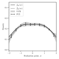
(a) Total degeneracy,
$\pi=\left(\frac{1}{2},0,\frac{1}{2}\right)$

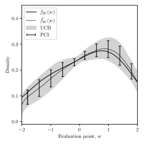
(b) Partial degeneracy,
$\pi=\left(\frac{1}{4},0,\frac{3}{4}\right)$

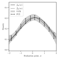
(c) No degeneracy,
$\pi=\left(\frac{1}{5},\frac{1}{5},\frac{3}{5}\right)$

Figure 2: Typical outcomes for three different values of the parameter $\pi$.

Next, Table 1 presents numerical results. For each degeneracy type (total, partial, none) and each kernel order ($p=2$, $p=4$), we run $2000$ repeats with sample size $n=3000$ (giving $N=4\,498\,500$ pairs of nodes) and with $d=50$ equally-spaced evaluation points. We record the average rule-of-thumb bandwidth $\widehat{h}_{\operatorname{ROT}}$ and the average root integrated mean squared error (RIMSE). For both the uniform confidence bands (UCB) and the pointwise confidence intervals (PCI), we report the coverage rate (CR) and the average width (AW). The lower-order kernel ($p=2$) ignores the bias, leading to good RIMSE performance and acceptable UCB coverage under partial or no degeneracy, but gives invalid inference under total degeneracy. In contrast, the higher-order kernel ($p=4$) provides robust bias correction and hence improves the coverage of the UCB in every regime, particularly under total degeneracy, at the cost of increasing both the RIMSE and the average widths of the confidence bands. As expected, the pointwise (in $w\in\mathcal{W}$) confidence intervals (PCIs) severely undercover in every regime. Thus our simulation results show that the proposed feasible inference methods based on robust bias correction and proper Studentization deliver valid uniform inference which is robust to unknown degenerate points in the underlying dyadic distribution.

Table 1: Numerical results for three values of the parameter $\pi$.

$\pi$	Degeneracy type	$\widehat{h}_{\operatorname{ROT}}$	$p$	RIMSE	UCB		PCI
					CR	AW	CR	AW
$\left(\frac{1}{2},0,\frac{1}{2}\right)$	Total	0.161	2	0.00048	87.1%	0.0028	6.5%	0.0017
			4	0.00068	95.2%	0.0042	9.7%	0.0025
$\left(\frac{1}{4},0,\frac{3}{4}\right)$	Partial	0.158	2	0.00228	94.5%	0.0112	75.6%	0.0083
			4	0.00234	94.7%	0.0124	65.3%	0.0087
$\left(\frac{1}{5},\frac{1}{5},\frac{3}{5}\right)$	None	0.145	2	0.00201	94.2%	0.0106	73.4%	0.0077
			4	0.00202	95.6%	0.0117	64.3%	0.0080

7 Application: counterfactual dyadic density estimation

To further showcase the applicability of our main results, we develop a kernel density estimator for dyadic counterfactual distributions. The aim of such counterfactual analysis is to estimate the distribution of an outcome variable had some covariates followed a distribution different from the actual one, and it is important in causal inference and program evaluation settings (DiNardo et al.,, 1996; Chernozhukov et al.,, 2013).

For each $r\in\{0,1\}$, let $\mathbf{W}_{n}^{r}$, $\mathbf{A}_{n}^{r}$ and $\mathbf{V}_{n}^{r}$ be random variables as defined in Assumption 2.1 and $\mathbf{X}_{n}^{r}=(X_{1}^{r},\ldots,X_{n}^{r})$ be some covariates. We assume that $(A_{i}^{r},X_{i}^{r})$ are independent over $1\leq i\leq n$ and that $\mathbf{X}_{n}^{r}$ is independent of $\mathbf{V}_{n}^{r}$, that $W_{ij}^{r}\mid X_{i}^{r},X_{j}^{r}$ has a conditional Lebesgue density $f_{W\mid XX}^{r}(\,\cdot\mid x_{1},x_{2})\in\mathcal{H}^{\beta}_{C_{\mathrm{H}}}(\mathcal{W})$, that $X_{i}^{r}$ follows a distribution function $F_{X}^{r}$ on a common support $\mathcal{X}$, and that $(\mathbf{A}_{n}^{0},\mathbf{V}_{n}^{0},\mathbf{X}_{n}^{0})$ is independent of $(\mathbf{A}_{n}^{1},\mathbf{V}_{n}^{1},\mathbf{X}_{n}^{1})$.

We interpret $r$ as an index for two populations, labeled $0$ and $1$. The counterfactual density of the outcome of population $1$ had it followed the same covariate distribution as population $0$ is

$$f_{W}^{1\triangleright 0}(w) =\mathbb{E}\left[f_{W\mid XX}^{1}\big{(}w\mid X_{1}^{0},X_{2}^{0}\big{)}\right]=\int_{\mathcal{X}}\int_{\mathcal{X}}f_{W\mid XX}^{1}(w\mid x_{1},x_{2})\psi(x_{1})\psi(x_{2})\,\mathrm{d}F_{X}^{1}(x_{1})\,\mathrm{d}F_{X}^{1}(x_{2}),$$

where $\psi(x)=\mathrm{d}F_{X}^{0}(x)/\mathrm{d}F_{X}^{1}(x)$ for $x\in\mathcal{X}$ is a Radon–Nikodym derivative. If $X^{0}_{i}$ and $X^{1}_{i}$ have Lebesgue densities, it is natural to consider a parametric model of the form $\mathrm{d}F_{X}^{r}(x)=f_{X}^{r}(x;\theta)\,\mathrm{d}x$ for some finite-dimensional parameter $\theta$. Alternatively, if the covariates $X_{n}^{r}$ are discrete and have a positive probability mass function $p_{X}^{r}(x)$ on a finite support $\mathcal{X}$, the object of interest becomes $f_{W}^{1\triangleright 0}(w)=\sum_{x_{1}\in\mathcal{X}}\sum_{x_{2}\in\mathcal{X}}f_{W\mid XX}^{1}(w\mid x_{1},x_{2})\psi(x_{1})\psi(x_{2})p_{X}^{1}(x_{1})p_{X}^{1}(x_{2})$, where $\psi(x)=p_{X}^{0}(x)/p_{X}^{1}(x)$ for $x\in\mathcal{X}$. We consider discrete covariates for simplicity, and hence the counterfactual dyadic kernel density estimator is

$$\widehat{f}_{W}^{\,1\triangleright 0}(w) =\frac{2}{n(n-1)}\sum_{i=1}^{n-1}\sum_{j=i+1}^{n}\widehat{\psi}(X_{i}^{1})\widehat{\psi}(X_{j}^{1})k_{h}(W_{ij}^{1},w),$$

where $\widehat{\psi}(x)=\widehat{p}_{X}^{\,0}(x)/\widehat{p}_{X}^{\,1}(x)$ and $\widehat{p}_{X}^{\,r}(x)=\frac{1}{n}\sum_{i=1}^{n}\mathbb{I}\{X_{i}^{r}=x\}$, with $\mathbb{I}$ the indicator function.

Section SA2.10 of the online supplemental appendix provides technical details: we show how an asymptotic linear representation for $\widehat{\psi}(x)$ leads to a modified Hoeffding-type decomposition of $\widehat{f}_{W}^{\,1\triangleright 0}(w)$, which is then used to establish that $\widehat{f}_{W}^{\,1\triangleright 0}$ is uniformly consistent for $f_{W}^{\,1\triangleright 0}(w)$ and also admits a Gaussian strong approximation, with the same rates of convergence as for the standard density estimator. Furthermore, define the covariance function of $\widehat{f}_{W}^{\,1\triangleright 0}(w)$ as $\Sigma_{n}^{1\triangleright 0}(w,w^{\prime})=\operatorname{Cov}\big{[}\widehat{f}_{W}^{\,1\triangleright 0}(w),\widehat{f}_{W}^{\,1\triangleright 0}(w^{\prime})\big{]}$, which can be estimated as follows. First let $\widehat{\kappa}(X_{i}^{0},X_{i}^{1},x)=\frac{\mathbb{I}\{X_{i}^{0}=x\}-\widehat{p}_{X}^{0}(x)}{\widehat{p}_{X}^{1}(x)}-\frac{\widehat{p}_{X}^{0}(x)}{\widehat{p}_{X}^{1}(x)}\frac{\mathbb{I}\{X_{i}^{1}=x\}-\widehat{p}_{X}^{1}(x)}{\widehat{p}_{X}^{1}(x)}$ be a plug-in estimate of the influence function for $\widehat{\psi}(x)$ and define the leave-one-out conditional expectation estimators
$S_{i}^{1\triangleright 0}(w)=\frac{1}{n-1}\big{(}\sum_{j=1}^{i-1}k_{h}(W_{ji}^{1},w)\widehat{\psi}(X_{j}^{1})+\sum_{j=i+1}^{n}k_{h}(W_{ij}^{1},w)\widehat{\psi}(X_{j}^{1})\big{)}$ and
$\widetilde{S}_{i}^{1\triangleright 0}(w)=\frac{1}{n-1}\sum_{j=1}^{n}\mathbb{I}\{j\neq i\}\widehat{\kappa}(X_{i}^{0},X_{i}^{1},X_{j}^{1})S_{j}^{1\triangleright 0}(w)$. Then define the covariance estimator

$$\widehat{\Sigma}_{n}^{1\triangleright 0}(w,w^{\prime}) =\frac{4}{n^{2}}\sum_{i=1}^{n}\big{(}\widehat{\psi}(X_{i}^{1})S_{i}^{1\triangleright 0}(w)+\widetilde{S}_{i}^{1\triangleright 0}(w)\big{)}\big{(}\widehat{\psi}(X_{i}^{1})S_{i}^{1\triangleright 0}(w^{\prime})+\widetilde{S}_{i}^{1\triangleright 0}(w^{\prime})\big{)}$$

$$\quad-\frac{4}{n^{3}(n-1)}\sum_{i<j}k_{h}(W_{ij}^{1},w)k_{h}(W_{ij}^{1},w^{\prime})\widehat{\psi}(X_{i}^{1})^{2}\widehat{\psi}(X_{j}^{1})^{2}-\frac{4}{n}\widehat{f}_{W}^{\,1\triangleright 0}(w)\widehat{f}_{W}^{\,1\triangleright 0}(w^{\prime}).$$

We use a positive semi-definite approximation to $\widehat{\Sigma}_{n}^{1\triangleright 0}$, denoted by $\widehat{\Sigma}_{n}^{+,1\triangleright 0}$, as in Section 5.1. To construct feasible uniform confidence bands, define a process $\widehat{Z}_{n}^{T,1\triangleright 0}(w)$ which is conditionally mean-zero and conditionally Gaussian given the data $\mathbf{W}_{n}^{1}$, $\mathbf{X}_{n}^{0}$ and $\mathbf{X}_{n}^{1}$ and whose conditional covariance structure is $\mathbb{E}\big{[}\widehat{Z}_{n}^{T,1\triangleright 0}(w)\widehat{Z}_{n}^{T,1\triangleright 0}(w^{\prime})\bigm{|}\mathbf{W}_{n}^{1},\mathbf{X}_{n}^{0},\mathbf{X}_{n}^{1}\big{]}=\frac{\widehat{\Sigma}_{n}^{+,1\triangleright 0}(w,w^{\prime})}{\sqrt{\widehat{\Sigma}_{n}^{+,1\triangleright 0}(w,w)\widehat{\Sigma}_{n}^{+,1\triangleright 0}(w^{\prime},w^{\prime})}}$. For $\alpha\in(0,1)$, define $\widehat{q}_{1-\alpha}^{\,1\triangleright 0}$ as the conditional quantile satisfying $\mathbb{P}\big{(}\sup_{w\in\mathcal{W}}\big{|}\widehat{Z}_{n}^{T,1\triangleright 0}(w)\big{|}\leq\widehat{q}_{1-\alpha}^{\,1\triangleright 0}\bigm{|}\mathbf{W}_{n}^{1},\mathbf{X}_{n}^{0},\mathbf{X}_{n}^{1}\big{)}=1-\alpha$. Then, assuming that the covariance estimator is appropriately consistent,

$$\mathbb{P}\left(f_{W}^{1\triangleright 0}(w)\in\left[\widehat{f}_{W}^{\,1\triangleright 0}(w)\pm\widehat{q}^{\,1\triangleright 0}_{1-\alpha}\sqrt{\widehat{\Sigma}_{n}^{+,1\triangleright 0}(w,w)}\,\right]\,\textup{for all }w\in\mathcal{W}\right)\to 1-\alpha,$$

giving feasible uniform inference methods, which are robust to unknown degeneracies, for counterfactual distribution analysis in dyadic data settings.

7.1 Application to trade data

We illustrate the performance of our estimation and inference methods with a real-world data set. We use international bilateral trade data from the International Monetary Fund’s Direction of Trade Statistics (DOTS), previously analyzed by Head and Mayer, (2014) and Chiang et al., (2023). This data set contains information about the yearly trade flows among $n=207$ economies ($N=21\,321$ pairs), and we focus on the years $1995$, $2000$ and $2005$.

We define the trade volume between countries $i$ and $j$ as the logarithm of the sum of the trade flow (in billions of US dollars) from $i$ to $j$ and the trade flow from $j$ to $i$. In each year several pairs of countries did not trade directly, yielding trade flows of zero and hence a trade volume of $-\infty$. We therefore assume that the distribution of trade volumes is a mixture of a point mass at $-\infty$ and a Lebesgue density on $\mathbb{R}$. The local nature of our estimator means that observations taking the value of $-\infty$ can simply be removed from the data set. Table 2 gives summary statistics for these trade networks, and shows how the networks tend to become more connected over time, with edge density, average degree and clustering coefficient all increasing.

Table 2: Summary statistics for the DOTS trade networks.

Year	Nodes	Edges	Edge density	Average degree	Clustering coefficient
1995	207	11 603	0.5442	112.1	0.7250
2000	207	12 528	0.5876	121.0	0.7674
2005	207	12 807	0.6007	123.7	0.7745

For counterfactual analysis we use the gross domestic product (GDP) of each country as a covariate, using $10\%$-percentiles to group the values into $10$ different levels for ease of estimation. This allows for a comparison of the observed distribution of trade at each year with, for example, the counterfactual distribution of trade had the GDP distribution remained as it was in $1995$. As such we can measure how much of the change in trade distribution is attributable to a shift in the GDP distribution.

To estimate the trade volume density function we use Algorithm 1 with $d=100$ equally-spaced evaluation points in $[-10,10]$, using the rule-of-thumb bandwidth selector $\widehat{h}_{\operatorname{ROT}}$ from Section 5.3 with $p=2$ and $C(K)=2.435$. For inference we use an Epanechnikov kernel of order $p=4$ and resample the Gaussian process $B=10\,000$ times. We also estimate the counterfactual trade distributions in 2000 and 2005 respectively, replacing the GDP distribution with that from 1995. For each year, Figure 3 plots the real and counterfactual density estimates along with their respective uniform confidence bands (UCB) at the nominal coverage rate of $95\%$. Our empirical results show that the counterfactual distribution drifts further from the truth in 2005 compared with 2000, indicating a more significant shift in the GDP distribution. In the online supplemental appendix we repeat the procedure using a parametric (log-normal maximum likelihood) preliminary estimate of the GDP distribution, and observe that the results are qualitatively similar.

(a) Year 1995, $\widehat{h}_{\operatorname{ROT}}=1.27$

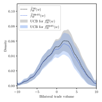
(b) Year 2000, $\widehat{h}_{\operatorname{ROT}}=1.31$

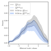
(c) Year 2005, $\widehat{h}_{\operatorname{ROT}}=1.37$

Figure 3: Real and counterfactual density estimates and confidence bands for the DOTS data.

8 Other applications and future work

To emphasize the broad applicability of our methods to network science problems, we present three application scenarios. The first concerns comparison of networks (Kolaczyk,, 2009), while the second and third involve nonparametric and semiparametric dyadic regression respectively.

Firstly, consider the setting where there are two independent networks with continuous dyadic covariates $\mathbf{W}_{n}^{0}$ and $\mathbf{W}_{m}^{1}$ respectively. Practitioners may wish to test if these two dyadic distributions are the same, that is, whether their density functions $f_{W}^{0}$ and $f_{W}^{1}$ are equal on their common support $\mathcal{W}\subseteq\mathbb{R}$. We present a family of hypothesis tests for this scenario based on dyadic kernel density estimation. Let $\widehat{f}_{W}^{\,0}(w)$ and $\widehat{f}_{W}^{\,1}(w)$ be the associated (bias-corrected) dyadic kernel density estimators. Consider the test statistics $\tau_{p}$ for $1\leq p\leq\infty$ where

$$\tau_{p} =\left(\int_{-\infty}^{\infty}\left|\widehat{f}_{W}^{\,1}(w)-\widehat{f}_{W}^{\,0}(w)\right|^{p}\,\mathrm{d}w\right)^{1/p}\text{ for }p<\infty,\text{ and }\,\tau_{\infty}=\sup_{w\in\mathcal{W}}\left|\widehat{f}_{W}^{\,1}(w)-\widehat{f}_{W}^{\,0}(w)\right|.$$ (4)

Clearly we should reject the null hypothesis that $f_{W}^{0}=f_{W}^{1}$ whenever the test statistic $\tau_{p}$ is sufficiently large. To estimate the critical value, let $\widehat{\Sigma}_{n}^{+,0}(w,w^{\prime})$ and $\widehat{\Sigma}_{m}^{+,1}(w,w^{\prime})$ be the positive semi-definite estimators defined in Section 5.1 and let $\widehat{Z}^{0}_{n}(w)$ and $\widehat{Z}^{1}_{m}(w)$ be zero-mean Gaussian processes with covariance structures $\widehat{\Sigma}_{n}^{+,0}(w,w^{\prime})$ and $\widehat{\Sigma}_{m}^{+,1}(w,w^{\prime})$ respectively, which are independent conditional on the data. Define the approximate null test statistic $\widehat{\tau}_{p}$ by replacing $\widehat{f}_{W}^{\,0}(w)$ and $\widehat{f}_{W}^{\,1}(w)$ with $\widehat{Z}^{0}_{n}(w)$ and $\widehat{Z}^{1}_{m}(w)$ respectively in (4). For a significance level $\alpha\in(0,1)$, the critical value is $\widehat{C}_{\alpha}$ where $\mathbb{P}\big{(}\widehat{\tau}_{p}\geq\widehat{C}_{\alpha}\bigm{|}\mathbf{W}_{n}^{0},\mathbf{W}_{n}^{1}\big{)}=\alpha$. This is estimated by Monte Carlo simulation, resampling from the conditional law of $\widehat{Z}^{0}_{n}(w)$ and $\widehat{Z}^{1}_{m}(w)$ and replacing integrals and suprema by sums and maxima over a finite partition of $\mathcal{W}$.

While our focus has been on density estimation with dyadic data, our uniform dyadic estimation and inference results are readily applicable to the settings of nonparametric and semiparametric dyadic regression. For our second example, suppose that $Y_{ij}=Y(X_{i},X_{j},A_{i},A_{j},V_{ij})$, where only $\mathbf{X}_{n}$ and $\mathbf{Y}_{n}$ are observed and $\mathbf{V}_{n}$ is independent of $(\mathbf{X}_{n},\mathbf{A}_{n})$, with $\mathbf{X}_{n}=(X_{i}:1\leq i\leq n)$, $\mathbf{A}_{n}=(A_{i}:1\leq i\leq n)$, $\mathbf{Y}_{n}=(Y_{ij}:1\leq i<j\leq n)$ and $\mathbf{V}_{n}=(V_{ij}:1\leq i<j\leq n)$. A parameter of interest is the regression function $\mu(x_{1},x_{2})=\mathbb{E}[Y_{ij}\mid X_{i}=x_{1},X_{j}=x_{2}]$, which can be used to analyze average or partial effects of changing the node attributes $X_{i}$ and $X_{j}$ on the edge variable $Y_{ij}$. This conditional expectation could be estimated using local polynomial methods: suppose that $X_{i}$ takes values in $\mathbb{R}^{m}$ and let $r(x_{1},x_{2})$ be a monomial basis up to degree $\gamma\geq 0$ on $\mathbb{R}^{m}\times\mathbb{R}^{m}$. Then, for some bandwidth $h>0$ and a kernel function $k_{h}$ on $\mathbb{R}^{m}\times\mathbb{R}^{m}$, the local polynomial regression estimator of $\mu(x_{1},x_{2})$ is $\widehat{\mu}(x_{1},x_{2})=e_{1}^{\mathsf{T}}\widehat{\beta}(x_{1},x_{2})$ where $e_{1}$ is the first standard unit vector in $\mathbb{R}^{q}$ for $q=\binom{2m+\gamma}{\gamma}$ and

$$\widehat{\beta}(x_{1},x_{2}) =\operatorname*{arg\,min}_{\beta\in\mathbb{R}^{q}}\sum_{i=1}^{n-1}\sum_{j=i+1}^{n}\left(Y_{ij}-r(X_{i}-x_{1},X_{j}-x_{2})^{\mathsf{T}}\beta\right)^{2}k_{h}(X_{i}-x_{1},X_{j}-x_{2})$$

$$=\left(\sum_{i=1}^{n-1}\sum_{j=i+1}^{n}k_{ij}r_{ij}r_{ij}^{\mathsf{T}}\right)^{-1}\left(\sum_{i=1}^{n-1}\sum_{j=i+1}^{n}k_{ij}r_{ij}Y_{ij}\right),$$ (5)

with $k_{ij}=k_{h}(X_{i}-x_{1},X_{j}-x_{2})$ and $r_{ij}=r(X_{i}-x_{1},X_{j}-x_{2})$. Graham et al., (2021) established pointwise distribution theory for the special case of the dyadic Nadaraya–Watson kernel regression estimator ($\gamma=0$), but no uniform analogues have yet been given. It can be shown that the “denominator” matrix in (5) converges uniformly to its expectation, while the U-process-like “numerator” matrix can be handled the same way as we analyzed $\widehat{f}_{W}(w)$ in this paper, through a Hoeffding-type decomposition and strong approximation methods, along with standard bias calculations. Such distributional approximation results can be used to construct valid uniform confidence bands for the regression function $\mu(x_{1},x_{2})$, as well as to conduct hypothesis testing for parametric specifications or shape constraints.

As a third example, we consider applying our results to semiparametric semi-linear regression problems. The dyadic semi-linear regression model is $\mathbb{E}[Y_{ij}\mid W_{ij},X_{i},X_{j}]=\theta^{\mathsf{T}}W_{ij}+g(X_{i},X_{j})$ where $\theta$ is the finite-dimensional parameter of interest and $g(X_{i},X_{j})$ is an unknown function of the covariates $(X_{i},X_{j})$. Local polynomial (or other) methods can be used to estimate $\theta$ and $g$, where the estimator of the nonparametric component $g$ takes a similar form to (5), that is, a ratio of two kernel-based estimators as in (1). Consequently, our strong approximation techniques presented in this paper can be appropriately modified to develop valid uniform inference procedures for $g$ and $\mathbb{E}[Y_{ij}\mid W_{ij}=w,X_{i}=x_{1},X_{j}=x_{2}]$, as well as functionals thereof.

9 Conclusion

We studied the uniform estimation and inference properties of the dyadic kernel density estimator $\widehat{f}_{W}$ given in (1), which forms a class of U-process-like estimators indexed by the $n$-varying kernel function $k_{h}$ on $\mathcal{W}$. We established uniform minimax-optimal point estimation results and uniform distributional approximations for this estimator based on novel strong approximation strategies. We then applied these results to derive valid and feasible uniform confidence bands for the dyadic density estimand $f_{W}$, and also developed a substantive application of our theory to counterfactual dyadic density analysis. We gave some other statistical applications of our methodology as well as potential avenues for future research. From a technical perspective, the online supplemental appendix contains several generic results concerning strong approximation methods and maximal inequalities for empirical processes that may be of independent interest.

Supplemental material

A supplemental appendix containing technical and methodological details as well as proofs and additional empirical results is available at https://arxiv.org/abs/2201.05967. Replication files for the empirical studies are provided at https://github.com/wgunderwood/DyadicKDE.jl.

References

- Aldous, (1981) Aldous, D. J. (1981). Representations for partially exchangeable arrays of random variables. Journal of Multivariate Analysis, 11(4):581–598.
- ApS, (2021) ApS, M. (2021). The MOSEK Optimizer API for C manual. Version 9.3.
- Belloni et al., (2019) Belloni, A., Chernozhukov, V., Chetverikov, D., and Fernández-Val, I. (2019). Conditional quantile processes based on series or many regressors. Journal of Econometrics, 213(1):4–29.
- Birgé, (2001) Birgé, L. (2001). An alternative point of view on Lepski’s method. Lecture Notes – Monograph Series, 36:113–133.
- Calonico et al., (2018) Calonico, S., Cattaneo, M. D., and Farrell, M. H. (2018). On the effect of bias estimation on coverage accuracy in nonparametric inference. Journal of the American Statistical Association, 113(522):767–779.
- Calonico et al., (2022) Calonico, S., Cattaneo, M. D., and Farrell, M. H. (2022). Coverage error optimal confidence intervals for local polynomial regression. Bernoulli, 28(4):2998–3022.
- Chernozhukov et al., (2017) Chernozhukov, V., Chetverikov, D., and Kato, K. (2017). Central limit theorems and bootstrap in high dimensions. The Annals of Probability, 45(4):2309–2352.
- Chernozhukov et al., (2014) Chernozhukov, V., Chetverikov, D., Kato, K., et al. (2014). Anti-concentration and honest, adaptive confidence bands. The Annals of Statistics, 42(5):1787–1818.
- Chernozhukov et al., (2013) Chernozhukov, V., Fernández-Val, I., and Melly, B. (2013). Inference on counterfactual distributions. Econometrica, 81(6):2205–2268.
- Chiang et al., (2023) Chiang, H. D., Kato, K., and Sasaki, Y. (2023). Inference for high-dimensional exchangeable arrays. Journal of the American Statistical Association, 118(543):1595–1605.
- Chiang and Tan, (2023) Chiang, H. D. and Tan, B. Y. (2023). Empirical likelihood and uniform convergence rates for dyadic kernel density estimation. Journal of Business and Economic Statistics, 41(3):906–914.
- Davezies et al., (2021) Davezies, L., D’Haultfœuille, X., and Guyonvarch, Y. (2021). Empirical process results for exchangeable arrays. The Annals of Statistics, 49(2):845–862.
- DiNardo et al., (1996) DiNardo, J., Fortin, N. M., and Lemieux, T. (1996). Labor market institutions and the distribution of wages, 1973–1992: A semiparametric approach. Econometrica, 64(5):1001–1004.
- Dudley, (1999) Dudley, R. M. (1999). Uniform Central Limit Theorems. Cambridge Studies in Advanced Mathematics. Cambridge University Press.
- Gao and Ma, (2021) Gao, C. and Ma, Z. (2021). Minimax rates in network analysis: Graphon estimation, community detection and hypothesis testing. Statistical Science, 36(1):16–33.
- Giné et al., (2004) Giné, E., Koltchinskii, V., and Sakhanenko, L. (2004). Kernel density estimators: convergence in distribution for weighted sup-norms. Probability Theory and Related Fields, 130(2):167–198.
- Giné and Nickl, (2010) Giné, E. and Nickl, R. (2010). Confidence bands in density estimation. The Annals of Statistics, 38(2):1122–1170.
- Giné and Nickl, (2021) Giné, E. and Nickl, R. (2021). Mathematical Foundations of Infinite-Dimensional Statistical Models. Cambridge Series in Statistical and Probabilistic Mathematics. Cambridge University Press.
- Graham, (2020) Graham, B. S. (2020). Network data. In Handbook of Econometrics, volume 7, pages 111–218. Elsevier.
- Graham et al., (2021) Graham, B. S., Niu, F., and Powell, J. L. (2021). Minimax risk and uniform convergence rates for nonparametric dyadic regression. Technical report, National Bureau of Economic Research.
- Graham et al., (2023) Graham, B. S., Niu, F., and Powell, J. L. (2023). Kernel density estimation for undirected dyadic data. Journal of Econometrics. forthcoming.
- Hall, (1992) Hall, P. (1992). Effect of bias estimation on coverage accuracy of bootstrap confidence intervals for a probability density. The Annals of Statistics, 20(2):675–694.
- Hall and Kang, (2001) Hall, P. and Kang, K.-H. (2001). Bootstrapping nonparametric density estimators with empirically chosen bandwidths. The Annals of Statistics, 29(5):1443–1468.
- Head and Mayer, (2014) Head, K. and Mayer, T. (2014). Gravity equations: Workhorse, toolkit, and cookbook. In Handbook of International Economics, volume 4, pages 131–195. Elsevier.
- Hoover, (1979) Hoover, D. N. (1979). Relations on probability spaces and arrays of random variables. Preprint, Institute for Advanced Study, Princeton, NJ.
- Kenny et al., (2020) Kenny, D. A., Kashy, D. A., and Cook, W. L. (2020). Dyadic Data Analysis. Guilford Publications.
- Kolaczyk, (2009) Kolaczyk, E. D. (2009). Statistical Analysis of Network Data: Methods and Models. Springer Series in Statistics. Springer, New York.
- Komlós et al., (1975) Komlós, J., Major, P., and Tusnády, G. (1975). An approximation of partial sums of independent RVs, and the sample DF. I. Zeitschrift für Wahrscheinlichkeitstheorie und verwandte Gebiete, 32(1-2):111–131.
- Laurent and Rendl, (2005) Laurent, M. and Rendl, F. (2005). Semidefinite programming and integer programming. In Discrete Optimization, volume 12 of Handbooks in Operations Research and Management Science, pages 393–514. Elsevier.
- Lepskii, (1992) Lepskii, O. V. (1992). Asymptotically minimax adaptive estimation. I: Upper bounds. optimally adaptive estimates. Theory of Probability & its Applications, 36(4):682–697.
- Luke and Harris, (2007) Luke, D. A. and Harris, J. K. (2007). Network analysis in public health: history, methods, and applications. Annual Review of Public Health, 28:69–93.
- Matsushita and Otsu, (2021) Matsushita, Y. and Otsu, T. (2021). Jackknife empirical likelihood: small bandwidth, sparse network and high-dimensional asymptotics. Biometrika, 108(3):661–674.
- Simonoff, (2012) Simonoff, J. S. (2012). Smoothing methods in statistics. Springer Science & Business Media.
- van der Vaart and Wellner, (1996) van der Vaart, A. W. and Wellner, J. A. (1996). Weak Convergence and Empirical Processes. Springer Series in Statistics. Springer, New York, NY.
- Wand and Jones, (1994) Wand, M. P. and Jones, M. C. (1994). Kernel Smoothing. CRC Press.
- Yurinskii, (1978) Yurinskii, V. V. (1978). On the error of the Gaussian approximation for convolutions. Theory of Probability & its Applications, 22(2):236–247.